1. Introduction
Growing dissidence over the causes and impacts of environmental change in the modern era has forced an ever-increasing need for data accuracy and certainty. Studied patterns of global change such as habitat augmentation, loss of biodiversity, invasive species spread, and other systems imbalances have designated humans as a ubiquitous disturbance for the natural world, leading to the current ‘Anthropocene’ era [
1,
2,
3]. Degrading natural systems also causes noted pressures on human economies and quality of life through diminished potential for ecosystem services [
4]. These services include life sustaining functions such as nutrient regulation, primary production products in agriculture and forestry, water quality management, and disease mitigation [
1,
2,
5]. Modeling natural systems requires us to undergo the inherently difficult task of finding representative characteristics. Forested landscapes comprising high compositional and structural diversity (i.e., complexity), such as those in the Northeastern United States, further impede these efforts [
6]. In many cases, land cover allows us this ability to represent fundamental constructs of the earth’s surface [
7]. We can then employ remote sensing as a tool to collect land cover data at scales sufficient to overcome environmental issues [
8,
9,
10].
Remote sensing provides the leading source of land use and land cover data, supported by its scales of coverage, adaptability, and prolific modifications [
7,
11,
12]. The classification of remote sensed imagery traditionally referred to as thematic mapping, labels objects and features in defined groups based on the relationship of their attributes [
13,
14]. This process incorporates characteristics reflected within the source imagery and motivations of the project, to recognize both natural and artificial patterns and increase our ability to make informed decisions [
13,
15,
16].
In the digital age, the process of image classification has most often been performed on a per pixel basis. Pixel-based classification (PBC) algorithms utilize spectral reflectance values to assign class labels based on specified ranges. More refined classification techniques have also been formed to integrate data such as texture, terrain, and observed patterns based on expert knowledge [
17,
18,
19].
Technologies have recently advanced to allow users a more holistic, human vision matching, approach to image analysis in the form of object-based image analysis (OBIA). Object-based classification (OBC) techniques work beyond individual pixels to distinguish image objects (i.e., polygons, areas, or features), applying additional data parameters to each individual unit [
10,
20,
21]. OBC methods can also benefit users by reducing the noise found in land cover classifications at high spatial resolution using class-defining thresholds of spectral variability and area [
22]. The specific needs of the project and the characteristics of the remote sensing data help guide the decision between which classification method would be most appropriate for creating a desired thematic layer [
15,
23].
Outside of the progression of classification algorithms, novel remote sensing and computer vision technologies have inspired new developments in high-resolution three-dimensional (3D) and digital planimetric modeling. Photogrammetric principles have been applied to simultaneously correct for sensor tilt, topographic displacement in the scene, relief displacement, and even lens geometric distortions [
24,
25]. To facilitate this process, Structure from Motion (SfM) software packages isolate and match image tie points (i.e., keypoints) within high-resolution images with sizeable latitudinal and longitudinal overlap to form 3D photogrammetric point clouds and orthomosaic models [
25,
26,
27]. Techniques for accurate and effective SfM modeling have been refined, even in complex natural environments, to expand the value of these products [
28,
29,
30].
The appropriate use of these emergent remote sensing data products establishes a need for understanding their accuracy and sources of error. Validating data quality is a necessary step for incorporating conclusions drawn from remote sensing within the decision-making process. Spatial data accuracy is an aggregation of two distinct characteristics: positional accuracy and thematic accuracy [
10]. Positional accuracy is the difference in locational agreement between a remotely sensed data layer and known ground points, calculated through Root Mean Square Error (RMSE) [
31]. Thematic accuracy expresses a more complex measure of error, evaluating the agreement for the specific labels, attributes, or characteristics between what is on the ground and the spatial data product, typically in the form of an error matrix [
10].
The immense costs and difficulty of validating mapping projects have brought about several historic iterations of methods for quantitatively evaluating thematic accuracy [
10]. Being once an afterthought, the assessment of thematic accuracy has matured from a visual, qualitative process into a multivariate evaluation of site-specific agreement [
10]. Site-specific thematic map accuracy assessments utilize an error matrix (i.e., contingency table or confusion matrix) to evaluate individual class accuracies and the relations among sources of uncertainty [
23,
32]. While positional accuracy holds regulated standards for accuracy tolerance, thematic mapping projects must establish their own thresholds for amount and types of justifiable uncertainty. Within thematic accuracy two forms of error exist: errors of commission (i.e., user’s accuracy) and errors of omission (i.e., producer’s accuracy) [
33]. Commission errors represent the user’s ability to accurately classify ground characteristics [
10]. Omission errors assesses if the known ground reference points have been accurately captured by the thematic layer for each class [
33]. For most uses, commission errors are favored because the false addition of area to classes of interest is of less consequence than erroneously missing critical features [
10]. The error matrix presents a robust quantitative analysis tool for assessing thematic map accuracy of classified maps created through both pixel-based and object-based classification methods.
Collecting reference data, whether using higher-resolution remotely sensed data, ground sampling, or previously produced sources, must be based on a sound statistical sample design. Ground sampling stands out as the most common reference data collection procedure. However, such methods generally come with an inherent greater associated cost. During the classification process, reference data can be used for two distinct purposes, depending on the applied classification algorithm. Reference data can be used to train the classification (training data), generating the decision tree ruleset which forms the thematic layer. Secondly, reference data are used as the source of validation (validation data) during the accuracy assessment. These two forms of reference data must remain independent to ensure the process is statistically valid [
10].
There are also multiple methods for collecting ground reference data, such as: visual interpretation of an area, GPS locational confirmation, or full-record data sampling with precise positioning. The procedures of several professional and scientific fields have been adopted to promote the objective and efficient collection of reference data. Forest mensuration provides such a foundation for obtaining quantifiable information in forested landscapes, with systematic procedures that can mitigate biases and inaccuracies of sampling [
34,
35]. For many decades now, forest mensuration (i.e., biometrics) has provided the most accurate and precise observations of natural characteristics through the use of mathematical principles and field-tested tools [
34,
35,
36]. To observe long-term or large area trends in forest environments, systematic Continuous Forest Inventory (CFI) plot networks have been established. Many national agencies (e.g., the U.S. Forest Service) have such a sampling design (e.g., Forest Inventory and Analysis (FIA) Program) for monitoring large land areas in a proficient manner [
37]. Despite these sampling designs for efficient and effective reference data collection, the overwhelming costs of preforming a statistically valid accuracy assessment is a considerable limitation for most projects [
10,
23].
The maturation of remote sensing technologies in the 21st century has brought with it the practicality of widespread Unmanned Aerial Systems (UAS) applications. This low-cost and flexible platform generates on-demand, high-resolution products to meet the needs of society [
38,
39]. UAS represent an interconnected system of hardware and software technologies managed by a remote pilot in command [
30,
40]. Progressing from mechanical contraptions, UAS now assimilate microcomputer technologies that allow them to operate for forestry sampling [
29,
41], physical geography surveys [
42], rangeland mapping [
43], humanitarian aid [
44], precision agriculture [
45], and many other applications [
12,
39,
46].
The added potential of the UAS platform has supported a wide diversity of data collection initiatives. UAS-SfM products provide analytical context beyond that of traditional raw imagery, with products including photogrammetric point clouds, Digital Surface Models (DSM), and planimetric (or orthomosaic) surfaces. While it is becoming increasingly common to use high-spatial resolution satellite imagery for reference data to assess maps generated from medium to coarse resolution imagery, UAS provide a new opportunity at even higher spatial resolutions. To properly apply the practice of using high-resolution remote sensing imagery as a source of validation data [
36,
47,
48], our research focuses on if UAS provide the potential for collecting thematic map accuracy assessment reference data of a necessary quality and operational efficiency to endorse their use. To do this, we evaluated the agreement between the UAS-collected samples and the ground-based CFI plot composition. Specifically, this pilot study investigated if UAS are capable of effectively and efficiently collecting reference data for use in assessing the accuracy of thematic maps created from either a (1) pixel-based or (2) object-based classification approach.
2. Materials and Methods
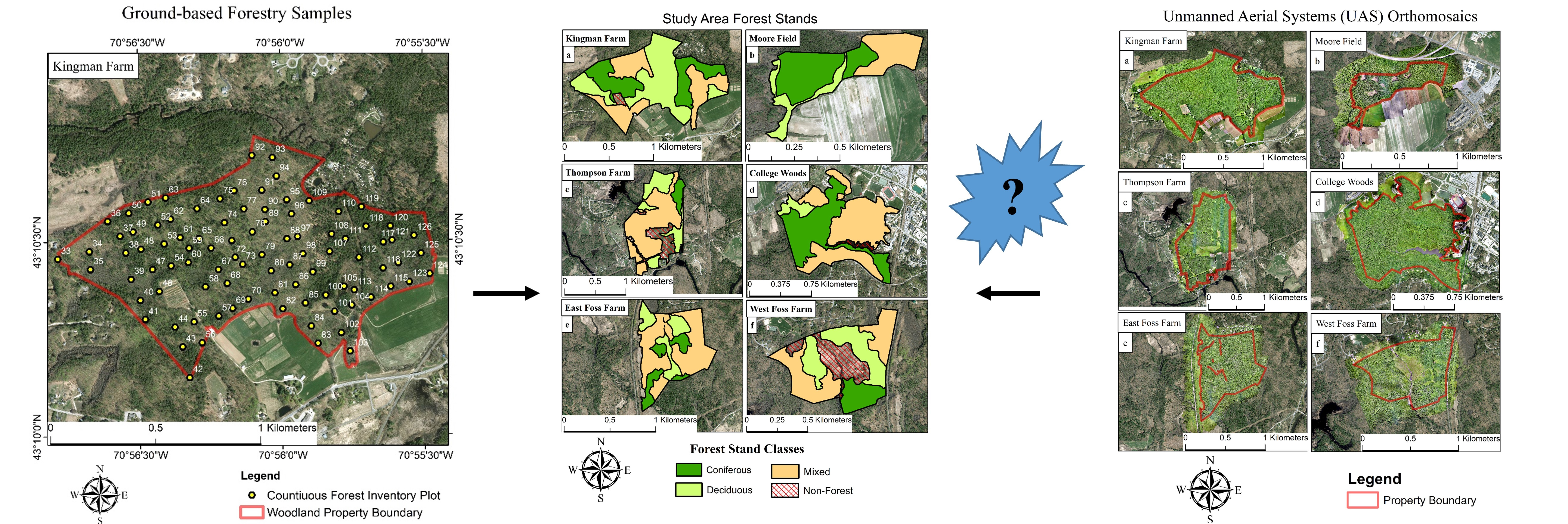
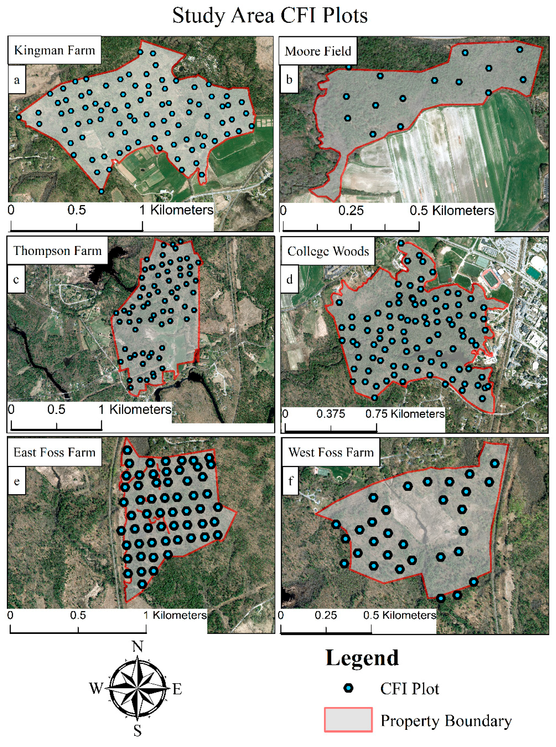
This research conducted surveys of six woodland properties comprising 522.85 ha of land, 377.57 ha of which were forest cover, in Southeastern New Hampshire (
Figure 1). The University of New Hampshire (UNH) owns and manages these six properties, as well as many others, to maintain research integrity for natural communities [
49]. These properties contain a wide diversity of structural and compositional diversity, ranging in size from 17 ha to 94.7 ha of forested land cover. Each property also contains a network of CFI plots for measuring landscape scale forest characteristics over time.
The systematic network of CFI ground sampling plots was established for each of the six woodland properties to estimate landscape level biophysical properties. These plot networks are sampled on a regular interval, not to exceed 10 years in reoccurrence. Kingman Farm presents the oldest data (10 years since previous sampling) and East Foss Farm, West Foss Farm, and Moore Field each being sampled most recently in 2014. CFI plots were located at one plot per hectare (
Figure 2), corresponding to the minimum management unit size. Each plot location used an angle-wedge prism sampling protocol to identify the individual trees to be included in the measurement at that location. Those trees meeting the optical displacement threshold (i.e., “in” the plot) were then measured for diameter at breast height (dbh), a species presence count, and the tree species itself, through horizontal point sampling guidelines [
35]. Prism sampling formed variable radius plots in relation to the basal area factor (BAF) applied. The proportional representation of species under this method is not unbiased with the basal area of the species with a larger dbh being overestimated, while those with smaller dbh are underestimated. Since photo interpretation of the plots is also performed from above this bias tends to hold here as well since the largest canopy trees are the ones most viewed. Therefore, the use of this sampling method is effective here.
The UNH Office of Woodland and Natural Areas forest technicians used the regionally recommended BAF 4.59 m
2 (or 20 ft
2) prism [
50]. Additionally, a nested plot “Big BAF” sampling integration applied a BAF 17.2176 m
2 (or 75 ft
2) prism to identify a subset of trees for expanded measurements. These ‘measure’ trees for had their height, bearing from plot center, distance from plot center, crown dimensions, and number of silvicultural logs present recorded.
Basal area was used to characterize species distributions and proportions throughout the woodland properties [
34,
35]. For our study, this meant quantifying the percentage of coniferous species basal area comprising each sample. For the six observed study areas a total of 31 tree species were observed (
Table S1). Instead of a species specific classification, our analysis centered on the conventional Deciduous Forest, Mixed Forest, and Coniferous Forest partitioning defined by Justice et al., [
5] and MacLean et al., [
6]. Here we used the Anderson et al., [
7] classification scheme definition for forests, being any area with 10 percent or greater aerial tree-crown density, which has the ability to produce lumber, and influences either the climate or hydrologic regime. From this scheme we defined:
“Coniferous” as any land surface dominated by large forest vegetation species, and managed as such, comprising an overstory canopy with a greater than or equal to 65% basal area per unit area coniferous species composition
“Mixed Forest” being any land surface dominated by large forest vegetation species, and managed as such, comprising an overstory canopy, which is less than 65% and greater than 25% basal area per unit area coniferous species in composition.
“Deciduous”, any land surface dominated by large forest vegetation species, and managed as such, comprising an overstory canopy, which is less than or equal to 25% basal area per unit area coniferous species in composition.
The presented classification ensured that samples were mutually exclusive, totally exhaustive, hierarchical, and produced objective repeatability [
7,
14].
The original ground-based datasets were collected for general-purpose analysis and research and so, needed to be cleaned, recoded, and refined using R Studio, version 3.3.2 [
51]. We used R Studio to isolate individual tree dbh measurements in centimeters and then compute basal area for the deciduous or coniferous species in centimeters squared. Of the original 359 CFI plots, six contained no recorded trees and were removed from the dataset, leaving 353 for analysis. Additionally, standing dead trees were removed due to the time lag between ground sampling and UAS operations. Percent coniferous composition by plot was calculated for the remaining locations based on the classification scheme.
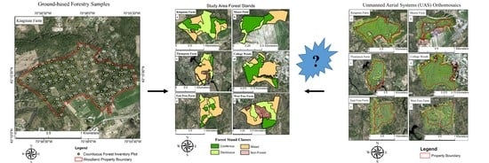
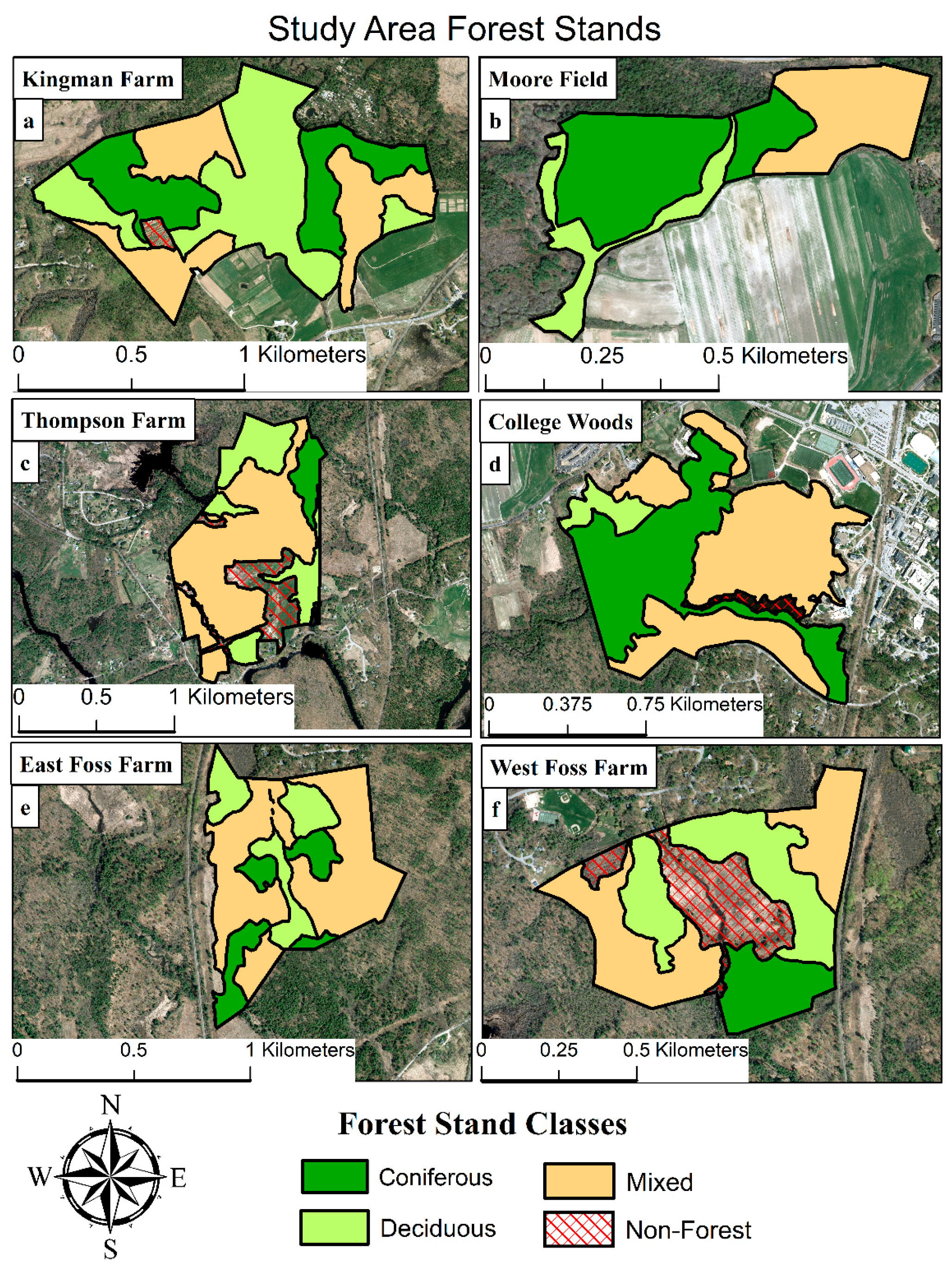
Once classified individually as either Coniferous, Mixed, or Deciduous in composition, the CFI plot network was used to delineate forest management units (stands). Leaf-off, natural color, NH Department of Transportation imagery with a 1-foot spatial resolution (0.3 × 0.3 m) [
52] provided further visual context for delineating the stand edges (
Figure 3). Non-managed forests and non-forested areas were also identified and removed from the study areas.
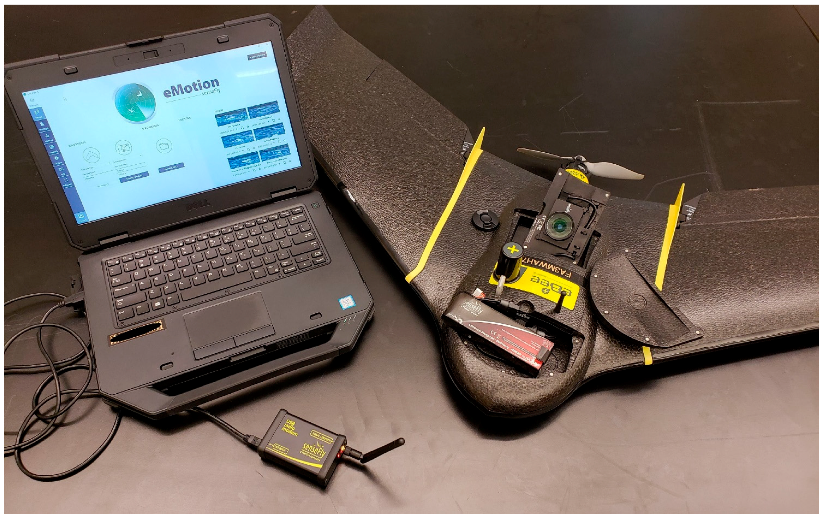
UAS imagery was collected using the eBee Plus (SenseFly Parrot Group, Cheseaux-sur-Lausanne, Switzerland), fixed-wing platform, during June and July 2017. The SenseFly eBee Plus operated under autonomous flight missions, in eMotion3 software version 3.2.4 (senseFly SA, Cheseaux-Lausanne, Switzerland), for approximately 45 minutes per battery. This system deployed the sensor optimized for drone applications (S.O.D.A), a 20 megapixel, 1in (2.54 cm) global shutter, natural color, proprietary sensor designed for photogrammetric analysis. In total, the system weighed 1.1 kg (
Figure 4).
UAS mission planning was designed to capture plot- and stand- level forest composition. Our team predefined mission blocks which optimized image collection while minimizing time outside of the study area. For larger properties (e.g., College Woods) up to six mission blocks were required based on legal restrictions to comprehensively image the study area. We used the maximum allowable flying height of 120 m above the forest canopy with an 85% forward overlap, and 75% side overlap for all photo missions [
30,
53]. This flying height was set relative to a statewide LiDAR dataset canopy height model provided by New Hampshire GRANIT [
54]. Further characteristics such as optimal sun angle (e.g., around solar noon), perpendicular wind directions, and consistent cloud coverage were considered during photo missions to maintain image quality and precision [
28,
30].
Post-flight processing began with joining the spatial data contained within the onboard flight log (.bb3 or .bbx) to each individual captured image. Next, we used Agisoft PhotoScan 1.3.2 [
55] for a high accuracy photo alignment, image tie point calibration, medium-dense point cloud formation, and planimetric model processing workflow [
30]. For all processing, we used a Dell Precision 7910, running an Intel Xeon E5-2697 v4 (18 core) CPU, with 64 GB of RAM, and a NVIDIA Quadro M4000 graphics card. Six total orthomosaics were created.
For each classification method, UAS reference data were extracted from the respective woodland property orthomosaic. West Foss Farm was used solely for establishing training data samples to guide the photo interpretation processes. In total, there were six sampling methods for comparing the ground-based and UAS derived reference data (
Table 1) (
Figures S1–S6).
For the first pixel-based classification reference data collection method (method one), 90 × 90 m extents were partitioned into 30 × 30 m grids, and positioned at the center of each forest stand. The center 30 × 30 m area then acted as the effective area for visually classifying the given sample. Using an effective area in this way both precluded misregistration errors between the reference data and the thematic layer, and ensured that the classified area was fully within the designated stand boundary [
10]. The second PBC reference data collection method (method two) used this same 90 × 90 m partitioned area but positionally aligned it with CFI-plot locations, avoiding overlaps with boundaries and other samples.
The first of four object-based classification reference data collection methods (method three) used a stratified random distribution for establishing a maximum number of 30 × 30 m interpretation areas (subsamples) within each forest stand. In total, 268 of these samples were created throughout 35 forest stands while remaining both spatially independent and maintaining at least two samples per forest stand. Similar to both PBC sampling methods, this and other OBC samples used 30 × 30 m effective areas for visually interpreting their classification. The second OBC reference data collection method (method four) used these previous 30 × 30 m classified areas as subsamples to represent the compositional heterogeneity at the image object (forest stand) level [
5,
10]. Forest stands which did not convey a clear majority, based on the subsamples, were classified based on a decision ruleset shown in
Table 2.
For the remaining two OBC reference data collection methods, we assessed individual 30 × 30 m samples (method five) and the overall forest stand classifications (method six) by direct comparison with the CFI-plots location compositions. An internal buffer of 21.215 m (the hypotenuse of the 30 × 30 m effective area) was applied to each forest stand to eliminate CFI-plots that were subject to stand boundary overlap. This process resulted in 202 subsamples for 28 stands within the interior regions of the five classified woodland properties.
For each of the six orthomosaic sampling procedures we relied on photo interpretation for deriving their compositional cover type classification. Using a confluence of evidence within the imagery, including morphological and spatial distribution patterns, the relative abundance of coniferous and deciduous species was identified [
24,
56]. Supporting this process was the training data collected from West Foss Farm (
Figure S7). A photo interpretation key was generated for plots with distinct compositional proportions, set at the distinctions between coniferous, deciduous, and mixed forest classes. During the visual classification process, a blind interpretation method was used so that ground data bias or location was not influential.
Error matrices were used to quantify the agreement between the UAS orthomosaic and ground-based thematic map reference data samples. Sample units for both PBC and OBC across all six approaches followed this method. These site-specific assessments reported producer’s, user’s, and overall accuracies for the five analyzed woodland properties [
33].
3. Results
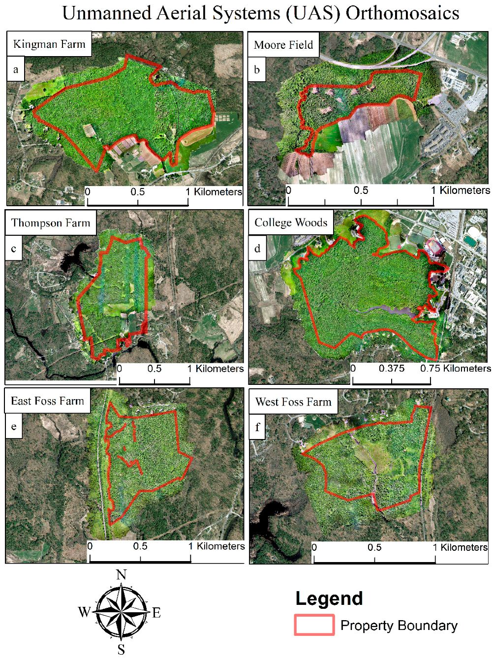
UAS imagery across the six woodland properties was used to generate six orthomosaics with a total land cover area of 398.71 ha. These UAS-SfM models represented 9173 images (
Figure 5). The resulting ground sampling distances (gsd) were: Kingman Farm at 2.86 cm, Moore Field at 3.32 cm, East Foss Farm at 3.54 cm, West Foss Farm at 3.18 cm, Thompson Farm at 3.36 cm, and College Woods at 3.19 cm, for an average pixel size of 3.24 cm. The use of Agisoft PhotoScan for producing these orthomosaics does not report XY positional errors. Additional registration of the woodland areas modeled to another geospatial data layer could determine relative error.
In our first analysis of pixel-based classification thematic map accuracy assessment reference data agreement, 29 sample units were located at the center of the forest stands. This method represented the photo interpretation potential of classifying forest stands from UAS image products. Overall agreement between ground-based and UAS-based reference data samples was 68.97% (
Table 3). Producer’s accuracy was highest for deciduous stands, while user’s accuracy was highest for coniferous forest stands.
For our second PBC reference data analysis, in which orthomosaic samples were registered with CFI-plot locations, 19 samples were assessed. Reference data classification agreement was 73.68% (
Table 4), with both user’s and producer’s accuracies highest for coniferous forest stands.
Four total OBC reference data error matrices were generated; two for the individual subsamples and two for the forest stands or image objects. Using the stratified random distribution for subsamples, our analysis showed an overall agreement of 63.81% between the ground-based forest stands and UAS orthomosaics across 268 samples. Producer’s accuracy was highest for deciduous forests while user’s accuracy was highest for mixed forest (
Table 5).
At the forest stand level, the majority agreement of the stratified randomly distributed subsamples presented a 71.43% agreement when compared to the ground-based forest stands (
Table 6). For the 35 forest stands analyzed, user’s accuracy was 100% for coniferous forest stands. Producer’s accuracy was highest for deciduous stands at 81.82%.
Next, UAS orthomosaic subsamples that were positionally aligned with individual CFI plots were assessed. A total of 202 samples were registered, with a 61.88% classification agreement (
Table 7). User’s accuracy was again highest for coniferous stands at 91.80%. Producer’s accuracy for these subsamples was highest in mixed forest, with an 80.85% agreement.
Forest stand level classification agreement, based on the positionally registered orthomosaic samples was 85.71%. In total, 28 forest stands were assessed (
Table 8). User’s and producer’s accuracies for all three classes varied marginally, ranging from 84.62% to 87.51%. Commission and omission error were both lowest for deciduous forest stands.
4. Discussion
This research set out to gauge whether UAS could adequately collect reference data for use in thematic map accuracy assessments, of both pixel-based and object-based classifications, for complex forest environments. To create UAS based comparative reference data samples, six independent orthomosaic models, totaling 398.71 ha of land area were formed from 9173 images (
Figure 5). The resulting average gsd was 3.24 cm. For the six comparative analyses of UAS and ground-based reference data (
Table 1), 581 samples were used.
Beginning with PBC, the resulting agreement for stratified randomly distributed samples was 68.97% (
Table 3). For this sampling technique, we experienced high levels of commission errors, especially between the coniferous and mixed forest types. One reason for this occurrence could have been the perceived dominance, visual bias, of the conifer canopies within the orthomosaic samples. Mixed forests experienced the greatest mischaracterization here. The CFI plot-registered PBC method generated a slightly higher overall accuracy at 73.68% (
Table 4). The mixed forest samples still posed issues for classification. Coniferous samples however, showed much improved agreement with ground-based classifications.
Next, we looked at the object-based classification reference data samples. Stratified randomly distributed subsamples had an agreement of 63.81% (
Table 5). While at the forest stand level agreement to the ground-based composition was 71.43% (
Table 6). As before, mixed forest samples showed the highest degree of error. CFI plot-registered OBC subsamples have a 61.88% agreement (
Table 7). For forest stand classifications based on these plot-registered subsamples, agreement was 85.71% (
Table 8). Mixed forests once again led to large amounts of both commission and omission error. Other than OBC subsample assessments, our results showed a continuously lower accuracy for the stratified randomly distributed techniques. The patchwork composition of the New England forest landscape could be a major reason for this difficulty.
As part of our analysis we wanted to understand the sources of intrinsic uncertainty for UAS reference data collection [
10,
18]. The compositional and structural complexity, although not to the degree of tropical forests, made working with even the three classes difficult. Visual interpretation was especially labored by this heterogeneity. To aid the interpretation process, branching patterns and species distribution trends were used [
24,
56]. All visual based classification was performed by the same interpreter, who has significant experience in remote sensing photo interpretation as well as local knowledge of the area. Another source of error could have been from setting fixed areas for UAS-based reference data samples while the CFI plots established variable radius areas [
35]. Our 30x30m effective areas looked to capture the majority of ground measured trees, providing snapshots of similarly sized sampling areas. Lastly, there were possible sources of error stemming from the CFI plot ground sampling procedures. Some woodlots, such as Kingman Farm, were sampled up to 10 years ago. Slight changes in composition could have occurred. Also, GPS positional error for the CFI plots was a considerable concern given the dense forest canopies. Error in GPS locations were minimized by removing points close to stand boundaries and by using pixel clusters when possible.
One of the first difficulties encountered in this project was in the logistics of flight planning. While most practitioners may strive for flight line orientation in a cardinal direction, we were limited at some locations due to FAA rules and abutting private properties [
30,
57]. As stated in the methods, UAS training missions and previously researched advice were used to guide comprehensive coverage of the woodland properties [
28]. A second difficulty in UAS reference data collection was that even with a sampling area of 377.57 ha, the minimum statistically valid sample size for a thematic mapping accuracy assessment was not reached [
10]. Forest stand structure and arrangement limited the number of samples for most assessments to below the recommended samples size of approximately 30 per class. A considerably larger, preferably continuous, forested land area would be needed to generate a sufficient sampling design. Limited sample sizes also brought into perspective the restriction from a more complex classification scheme. Although some remote sensing studies have performed to a species-specific classification, Justice et al., [
5] and MacLean et al., [
6] have both shown that a broader, three class, scheme has potential for understanding local forest composition.
Despite the still progressing nature of UAS data collection applications, this study has made the potential for cost reductions apparent. The volume of data collected and processed in only a few weeks opened the door for potential future research in digital image processing and computer vision. Automated classification processing, multiresolution segmentation [
20], or machine learning were a consideration but could not be implemented in this study. A continuing goal is to integrate the added context of the digital surface model (DSM), texture, and multispectral image properties into automated forest classifications. We hope that in future studies more precise ground data can be collected, to alleviate the positional registration error and help match exact trees. Additionally, broader analyses should be conducted to establish a comparison for UAS-based reference data to other forms of ground-based sampling protocols (e.g., FIA clustered sampling or fixed-area plots). Lastly, multi-temporal imagery could benefit all forms of UAS classification and should be studied further.
In well under a months’ time, this pilot study collected nearly 400 ha of forest land cover data to a reasonable accuracy. With added expert knowledge-driven interpretation or decreased landscape heterogeneity, this platform could prove to be a significant benefit to forested area research and management. Dense photogrammetric point clouds and ultra-high-resolution orthomosaic models were obtained, with the possibility of incorporating multispectral imagery in the future. These ultra-high resolution products have the potential now to provide an accessible alternative to reference data collected using high-spatial resolution satellite-based imagery. For the objective of collecting reference data which can train and validate environmental models, it must be remembered that reference data itself is not without intrinsic error [
58]. As hardware and software technologies continue to improve, the efficiency and effectiveness of these methods will continue to grow [
39]. UAS positional accuracy assessment products are gaining momentum [
12,
59,
60]. Providing examples to the benefits of UAS should also support further legislative reform, better matching the needs of practitioners. FAA RPIC guidelines remain a sizeable limitation for UAS mapping of continuous, remote, or structurally complex areas [
39,
57,
61]. We should also remember that these technologies should be used to augment and enhance data collection initiatives, and not replace the human element in sampling.


