Article

Forest Phenology Dynamics to Climate Change and Topography in a Geographic and Climate Transition Zone: The Qinling Mountains in Central China

1
College of Environment and Planning, Ministry of Education Key Laboratory of Geospatial Technology for Middle and Lower Yellow River Regions, Henan Collaborative Innovation Center of Urban-Rural Coordinated Development, Henan University, Kaifeng 475004, China
2
United States Department of Agriculture-Agricultural Research Service, Genetics and Sustainable Agriculture Research Unit, Highway, MS 39762, USA
3
Department of Geogsciences, Mississippi State University, Starkville, MS 39762, USA
4
United States Department of Agriculture, Forest Service, Brooklyn, MS 39762, USA
5
College of Science, Engineering and Health, Royal Melbourne Institute of Technology (RMIT) University, 124 LaTrobe Street, Melbourne, VIC 3000, Australia
*
Author to whom correspondence should be addressed.
Submission received: 22 September 2019 / Revised: 27 October 2019 / Accepted: 8 November 2019 / Published: 11 November 2019

Abstract

:
Forest ecosystems in an ecotone and their dynamics to climate change are growing ecological and environmental concerns. Phenology is one of the most critical biological indicators of climate change impacts on forest dynamics. In this study, we estimated and visualized the spatiotemporal patterns of forest phenology from 2001 to 2017 in the Qinling Mountains (QMs) based on the enhanced vegetation index (EVI) from MODerate-resolution Imaging Spectroradiometer (MODIS). We further analyzed this data to reveal the impacts of climate change and topography on the start of the growing season (SOS), end of the growing season (EOS), and the length of growing season (LOS). Our results showed that forest phenology metrics were very sensitive to changes in elevation, with a 2.4 days delayed SOS, 1.4 days advanced EOS, and 3.8 days shortened LOS for every 100 m increase in altitude. During the study period, on average, SOS advanced by 0.13 days year−1, EOS was delayed by 0.22 days year−1, and LOS increased by 0.35 day year−1. The phenological advanced and delayed speed across different elevation is not consistent. The speed of elevation-induced advanced SOS increased slightly with elevation, and the speed of elevation-induced delayed EOS shift reached a maximum value of 1500 m from 2001 to 2017. The sensitivity of SOS and EOS to preseason temperature displays that an increase of 1 °C in the regionally averaged preseason temperature would advance the average SOS by 1.23 days and delay the average EOS by 0.72 days, respectively. This study improved our understanding of the recent variability of forest phenology in mountain ecotones and explored the correlation between forest phenology and climate variables in the context of the ongoing climate warming.

1. Introduction

Research on phenology focuses on the phases of recurring biological life cycles, how these cycles are influenced by biotic and abiotic drivers and the interrelations among the same or different species [1]. Forest phenology is one of the most reliable biological indicators for evaluating the impacts of global warming in temperate and boreal zones because of its high sensitivity to climate change [2]. In turn, variations in forest phenology strongly affect the fitness and distribution of temperate and boreal forests [3] and, thus, the interspecific interactions among plants [4], ecosystem structure and function by varying the length of growing season [5,6], terrestrial ecosystem water and carbon balances [7,8], and climate system energy balances [9]. However, the processes underlying forest phenology are still unclear and need further research as they are essential to enhance the understanding of forest ecosystems and their responses to climate change.
Global warming has become an undeniable fact in recent years, changing the timings of plant flowering, leaf-out, growth stages, and leaf senescence over the past few decades [10]. Extensive research primarily focused on the start of the growing season (SOS) and found an earlier SOS in high latitudes and high altitudes based on the ground observations, satellite remote sensing, and model simulations [11,12,13,14,15,16,17]. However, the SOS trend diverges significantly among previous studies [18,19,20]. Due to the complexity and perplexity of vegetation phenological processes during autumn, studies on the processes of the end of the growing season (EOS) and its associated control factors have not received sufficient attention [21,22]. As the final phase of the plants’ seasonal cycle, EOS serves as an important occasion to recycle nutrients from senescing leaves to other plant tissues to sustain their growth in the following spring [23,24]. The EOS was recognized to be as important as the SOS in influencing the interannual variability of the carbon balance by controlling the length of the photosynthetically active period [10,25,26]. Therefore, combining the SOS, EOS, and length of the growing season (LOS) for vegetation and its associated environmental factors will improve our understanding of the response of vegetation to climate change.
Temperature is a primary climatic factor regulating the SOS and EOS in temperate and boreal forests. Recent studies have indicated that spring warming directly regulates the SOS, and the winter chilling requirement for dormancy release indirectly regulates the SOS [13]. Warming during summer and autumn can significantly delay the EOS [27], but the response of EOS to warming differed among species [28]. The warming trends also affect the time of phenology; for example, many studies show that phenology trends are significantly faster pre-1990 than post-2000 [19,20,29,30]. The EOS has a different temperature sensitivity compared with SOS; for example, the EOS response to temperature is larger than that of SOS [27]. Precipitation has also been found to be a primary driving factor affecting the SOS and EOS in a complex manner in temperate and boreal forests [11,12,31,32,33,34]. For example, Fu et al. [12] found that winter precipitation has a positive correlation with the heat requirement for SOS at northern middle and high latitudes. Precipitation also has a considerable impact on the EOS, particularly for arid and semi-arid regions [31]. Therefore, understanding the response of forest phenology to climate change is valuable. However, the processes underlying the forest phenology, which may differ among regions and ecosystems due to their associated climatic factors and the complex response of spring and autumn phenology to climate change in the mountains, are still not fully understood.
Mountain forests typically cover a concentrated and abundant vertical band spectrum of biological climates, providing important ecological service functions in maintaining biological diversity, regulating regional climate, and conserving water [35]. The elevational gradients can be treated as space-for-time substitutions to evaluate the influences of climate change on forest ecosystems. The environmental gradient of mountainous systems is unique, making it a sensitive indicator of climate change, and has become a focus for current climate change research. Meanwhile, warming trends may vary across the bioclimatic gradient, with stronger trends at higher latitudes and altitudes [36,37]. Therefore, biomes at high elevations are experiencing a more rapid change in temperature than those at low elevations [36]. Recent studies have shown trends of earlier SOS and delayed EOS in many mountain zones, including the Greater Khingan Mountains [38], the Changbai Mountains [39], the Andes Mountains [40], and semi-arid mountain regions [41], indicating that rising temperature could influence the phenological metrics. However, there is a lack of answers to whether the phenological advancement along different elevation gradients is uniform or diverse and how is the dynamics of uniform or diverse.
Satellite-based information has been used for monitoring the spatial heterogeneity of land surface phenology over recent decades and for discerning the spatiotemporal patterns of land surface phenology responding to the effects of climatic change [13,42]. Recent studies have effectively described the vegetation phenology using fine-resolution (<30 m), which can be achieved from fusing spare fine-and frequency medium-resolution images [43], from multiple years into a single synthetic year [44], and from optical HJ-1 satellites [45] and Sentinel-2 [46]. Although finer-resolution sensors are more effective for capturing the heterogeneous land cover, such sensors usually need longer revisit times with too few cloud-free images to effectively capture the seasonal changes in greenness [47]. According to the spatiotemporal resolutions and the length of time series, three satellite sensors, namely, Moderate Resolution Imaging Spectroradiometer (MODIS), Système Pour I’Observation de la Terre (SPOT), and Advanced Very High Resolution Radiometer (AVHRR), have often been used to monitor vegetation phenology [16,34]. Vegetation indices (e.g., EVI, Enhanced Vegetation Index; NDVI, Normalized Difference Vegetation Index) based on the spectral reflectance of vegetation are well correlated with chlorophyll abundance, photosynthetically active biomass, and energy absorption [48,49,50]. The EVI, which could avoid the problem of NDVI saturation in high vegetation coverage areas and reduce the effects of atmospheric and soil background, has proven to be a robust indicator of vegetation growth [51]. Therefore, a MODIS EVI dataset with a 500 m spatial resolution and an 8-day temporal resolution was used in this study for retrieving the forest phenology in the Qinling Mountains (QMs), China, taking into account the heterogeneity of the mountains and NDVI saturation in areas of dense forest coverage.
The QMs are located in a typical and important ecological and geographical transition zone in China. The transitional nature of the physical conditions, which is sensitive to external interference, provides an ideal region for examining the climatic and altitudinal effects on forest phenology metrics that is, hence, ideal for understanding the response of the regional forest ecosystems to ongoing global warming. We hypothesize that (1) the recent climate change has altered the forest growing season in the QMs, but the changes in SOS, EOS, and LOS along different elevation gradients are uneven; (2) temperature and precipitation are the key driving factors for SOS and EOS in the QMs. In this study, we investigated the relationships between topography, climate factors, and forest phenological metrics. In particular, we aim to (i) quantify the spatial pattern and interannual variability of the forest SOS, EOS, and LOS in the QMs from 2001 to 2017; (ii) evaluate the influence of elevation gradients on SOS, EOS, and LOS on a spatiotemporal scale; and (iii) explore the relationships between climatic factors (e.g., temperature, precipitation) and the spatiotemporal variations of forest phenology metrics.

2. Materials and Methods
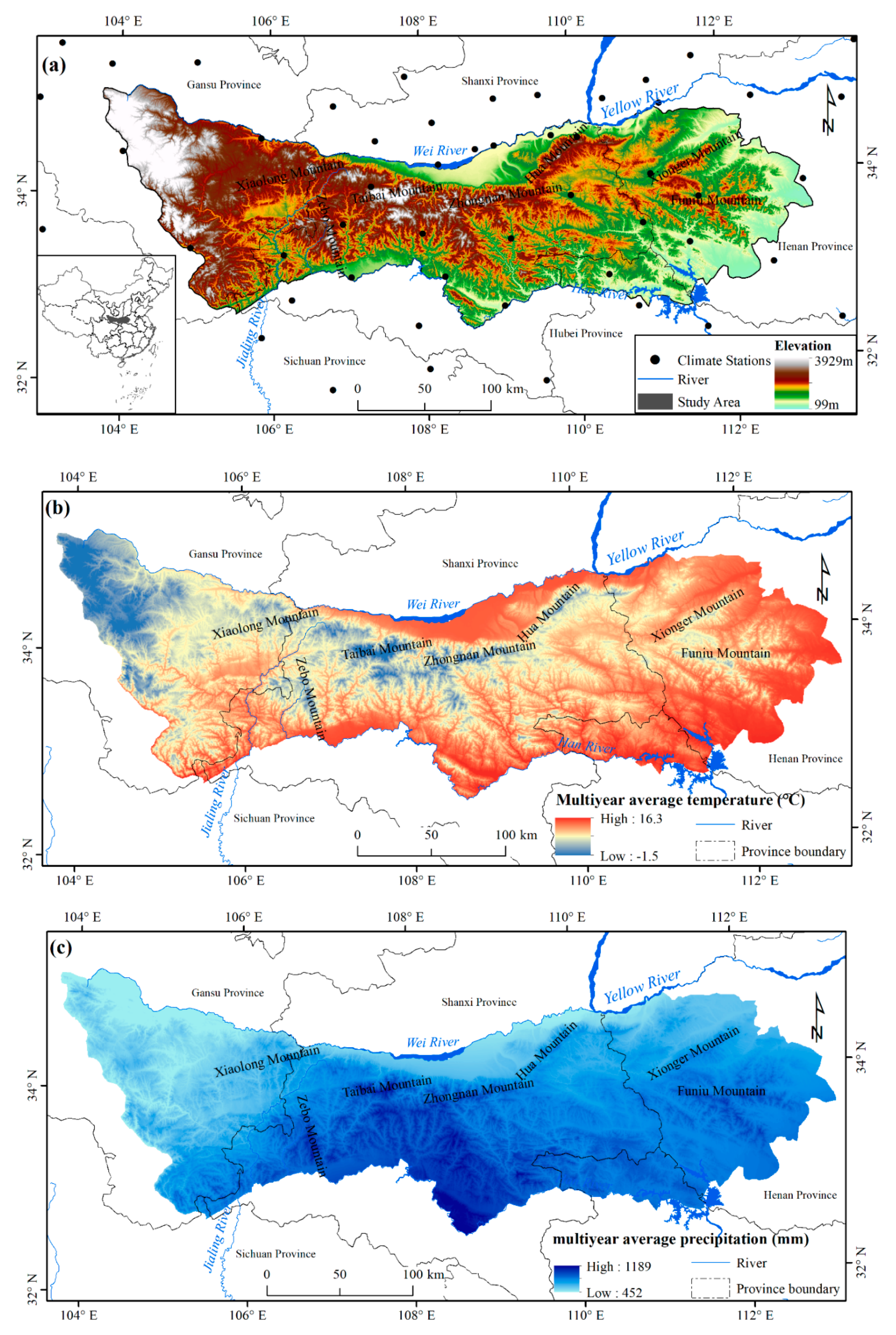
2.1. Study Area

The QMs is located in central China (Figure 1a), and it features important geographical transitions from a subtropical climate in the south to a warm-temperate climate in the north. The area contains a set of important geographical boundaries, including a boundary between the north and south, a 0 °C isotherm in January, an 800 mm isohyet, and an isoline of 2000 h of sunshine duration [52]. The annual mean temperature is −1.5~16.3 °C from high to low altitudes (Figure 1b), the cumulative precipitation is 452–1189 mm from north to south (Figure 1c), and the frost-free period is 200–250 days. The QMs include Xiaolong Mountain in Gansu Province, Taibai Mountain and Hua Mountain in Shanxi Province, and Xionger Mountain and Funiu Mountain in Henan Province (Figure 1). The mountains form the divide between the Yangtze River and the Yellow River and are adjacent to the Han River in the south and the Wei River in the north. Under the influence of topographical differentiation, different vegetation types dominate at different elevations covering accordingly along the south and north slopes of the QMs. The farming area is distributed from the elevation about 200 to 700 m, from 700 to 1300 m a deciduous broad-leaved forest belt grows, a deciduous oak forest belt grows above 1300 to about 2300 m, from 2300 to 2800 m a typical birch forest belt grows, a coniferous forest belt grows beyond 2800 to about 3200 m, and above 3200 m is the highest forest ecosystem of an alpine shrub-meadow belt. Because of the significant climate differences between the south and north of the QMs, there is a mildly different distributional spectrum of vegetation types [53].

2.2. MODIS EVI Dataset

The study area falls in MODIS path 26/row 05 and path 27/row 05. At each path/row, MOD09A1 scenes acquired in an annual year, with a temporal resolution of 8 days and a spatial resolution of 500 m from 2001 to 2017, were downloaded from the publicly available website of the USGS (United States Geological Survey) EROS (Earth Resources Observation and Science) [54]. Based on the heterogeneity of the Mountains, we selected the higher spatial resolution of 500 m with the maximum temporal resolution of 8 days. The original EVI data were mosaicked and reprojected from a sinusoidal projection to the Lambert Azimuthal Equal Area Projection. Each composite was clipped for the QMs area using the MODIS Reprojection Tool (MRT), and then, sequentially, were stacked to generate the yearly time-series dataset.

2.3. Climate Data

The meteorological dataset used in this study included daily mean temperature and cumulative precipitation from 2001 to 2017, which were downloaded from the China Meteorological Data Sharing Service System (http://data.cma.cn/). To obtain reliable spatially distributed climate data, 57 stations were selected covering not only the QMs but also the neighboring counties distributed throughout the south of Shanxi province, the southeast of Gansu province, the north of Sichuan province, the northwest of Hubei province, and the west of Henan province (Figure 1). The daily meteorological observations for all the sites from 2001 to 2017 were used to obtain the monthly mean temperature and cumulative precipitation. To analyze the correlation between the phenology metrics and the climate data, the ANUSPLIN method [55], which measures topographical effects on spatial climate interpolation [36], was used to interpolate and rasterize monthly climate data from the stations into 500 × 500 m grids to match the spatial resolution of EVI.

2.4. Auxiliary Data

To analyze the topographic effects of phenology metrics, we downloaded SRTM (Shuttle Radar Topography Mission) DEM (digital elevation model) data, with a 90 m spatial resolution, from the CGIAR (Consultative Group for International Agriculture Research) Consortium for Spatial Information website (http://srtm.csi.cgiar.org/). Using the mean algorithm, the SRTM (90 m) imagery was resampled into a new image with a cell size of 500 m to match the cell size of EVI. Elevation was also used as a co-variable in the ANUSPLIN method.
To overcome the mosaic effect of MODIS land cover (MOD12Q1), we used Globeland30, which is a global land cover at a 30 m resolution with good performance in classification accuracy [56,57]. Globeland30 was downloaded from a webpage (http://www.globallandcover.com/GLC30Download), and it was then resampled to 500 m to match the aforementioned EVI data, using the majority method.

2.5. Phenology Metrics Extraction

The EVI time series are often hindered by the poor quality of the original datasets due to various factors, for example, haze and cloud contamination and atmospheric absorption. To suppress atmospheric effects, EVI was composited by the Maximum Value Compositing (MVC) algorithm. Although MVC is surprisingly effective in reducing noise in EVI data, it cannot remove all the noise. However, the seasonal forest canopy EVI data tend to change gradually from a seasonal perspective. Thus, it is necessary to adopt a filter method to eliminate the negative influence, to interpolate the missing value, and finally to construct new EVI time-series datasets before extracting seasonal phenology metrics.
In general, the types of input data and desired results determine the choice of the smoothing method. The HANTS (Harmonic ANalysis of Time Series) method, which can fully consider the plant growth cycle and the dual characteristics of the data themselves, is an effective analysis approach. This approach has been widely used to reconstruct the EVI time series and NDVI time series for the past 20 years [58,59]. The HANTS algorithm is applied using an iterative way (for more detail on the curve fitting, see Roerink, Menenti, and Verhoef [58]).
In our analysis of EVI from 2001 to 2017, the HANTS parameters (the definition of the parameters can be found in Supplementary (Text1) were set as follows: (1) the number of frequency is 2, (2) the suppression flag is low, (3) the invalid data are 0 for low threshold and 1 for high threshold, (4) the fit error tolerance is 0.05, (5) the degree of over-determinedness is 5, and (6) the damping factor is 0.5. The 8-day EVI data were interpolated to daily timesteps in order to capture the rapid changes in land surface phenology. Then, the phenology metrics (SOS, EOS) were extracted based on the reconstructed EVI time series (Figure S1). Regarding the extraction of phenology metrics, it is difficult to define a single set of smoothing, and phenology metrics extraction methods can work with all different ecosystems and across all different kinds of remotely sensed data [60,61]. In this study, we chose the smoothing method of HANTS and the relative threshold method, which was successfully applied to the QMs [52]. The dates of SOS or EOS were defined, using the relative threshold method, as the times at which EVI values increased (SOS) or decreased (EOS) to a certain proportion of the seasonal amplitude, in the left or the right edge of the annual curve of EVI [34,62]. The LOS is equal to the difference between the EOS and the SOS. Such threshold values were determined according to the lowest absolute error between the leaf-out and leaf senescence dates measured in situ by the National Geographic Resource Science Data Center, National Science and Technology Infrastructure of China, National Earth System Science Data Sharing Infrastructure (http://gre.geodata.cn), and the remotely sensed phenology metrics (Figure S2). Ultimately, 30% of the amplitude was used to extract the dates of SOS and EOS, respectively, at both sides of the annual curve for each pixel.

2.6. Trend Analysis of the Phenology Metrics

We computed the mean annual EVI profile. Then, we analyzed the spatiotemporal variation trends of phenology metrics (SOS, EOS, and LOS), from 2001 to 2017, by means of a linear regression method. The linear trends (slope and p-value) are calculated based on pixel-by-pixel between the phenology metrics and years sequence. The slope is calculated as:
s l o p e = n × i = 1 n j × P j ( i = 1 n j ) ( i = 1 n P j ) n × i = 1 n j 2 ( i = 1 n j ) 2
where slope represents the temporal trend of the changes of land surface phenology, n = 17 is the total years of the monitoring period, and Pj (j = 1, 2, and 3) is the phenology metric (SOS, EOS, or LOS). Negative slopes indicate advanced SOS and EOS and shorter LOS, while positive slopes indicate delayed SOS and EOS and longer LOS. Thirdly, we further investigated how these spatially heterogeneous trends of the altitudinal gradient influenced the phenology metrics (SOS, EOS, and LOS) and tried to examine the differences in phenological responses along with elevation effects.

2.7. Determination of the Preseason of Forest Phenology

The temperatures in the preceding months are known to control the timing of spring leaf-out [15] and leaf senescence [21]. To define the length of the preseason whose mean temperature and accumulated precipitation had the most influence on SOS (or EOS), we analyzed the correlation coefficients between SOS (or EOS) and mean temperature and accumulated precipitation during 0, 1, 2, … n months before the multiyear averaged SOS (or EOS) using Spearman’s rank correlation coefficients. The preseason for mean temperature was defined by the highest absolute correlation coefficient between mean temperature and the multiyear averaged SOS (or EOS) [13,15,21]. We obtained the length of the preseason for precipitation in the same way but replacing the mean temperature with accumulated precipitation. The length of the preseason for SOS (or EOS) was defined as Lsos or (Leos). After that, we applied a temporal partial correlation analysis between the SOS (or EOS) and preseason mean temperature (accumulated precipitation), controlling for corresponding accumulated precipitation (mean temperature) during 2001–2017. The preseason of SOS is generally from the preceding November to the multiyear mean date of SOS [15], and the preseason of EOS is generally from June to the multiyear mean date of EOS [21,63].

2.8. Analysis of the Climate Change Impact on Phenology

Partial correlation analyses were used to reveal the relationship between each dependent and independent variable, excluding the confounding effects of other variables [49,64]. In this study, the pixel-based approach was used to analyze the partial correlation of forest phenology metrics and climatic factors (e.g., mean temperature, cumulated precipitation) in the preseason before each phenology metric. Considering the cumulative effect of climatic factors on SOS (or EOS), we obtained the largest significant partial correlation coefficient between the SOS (or EOS) and the temperature in n-month, after controlling the remaining corresponding EOS (or SOS) and precipitation. For instance, if the n-month temperature had the highest correlation with SOS (or EOS), the cumulative effect of temperature on SOS (or EOS) for this pixel would be treated as n months. In other words, at each pixel, the continuous n months before SOS (or EOS) (comprising the SOS (or EOS) appearing month) are the most important hints to trigger SOS (or EOS). We obtained the cumulative effect of precipitation on SOS (or EOS) in the same way but replacing the mean temperature with accumulated precipitation. The partial correlations between SOS (or EOS) and the preseason mean temperatures and cumulative precipitations were assessed at a 95% confidence level during 2001–2017. The statistical significance of the partial correlation coefficient was evaluated by using the Student’s t-test.

3. Results

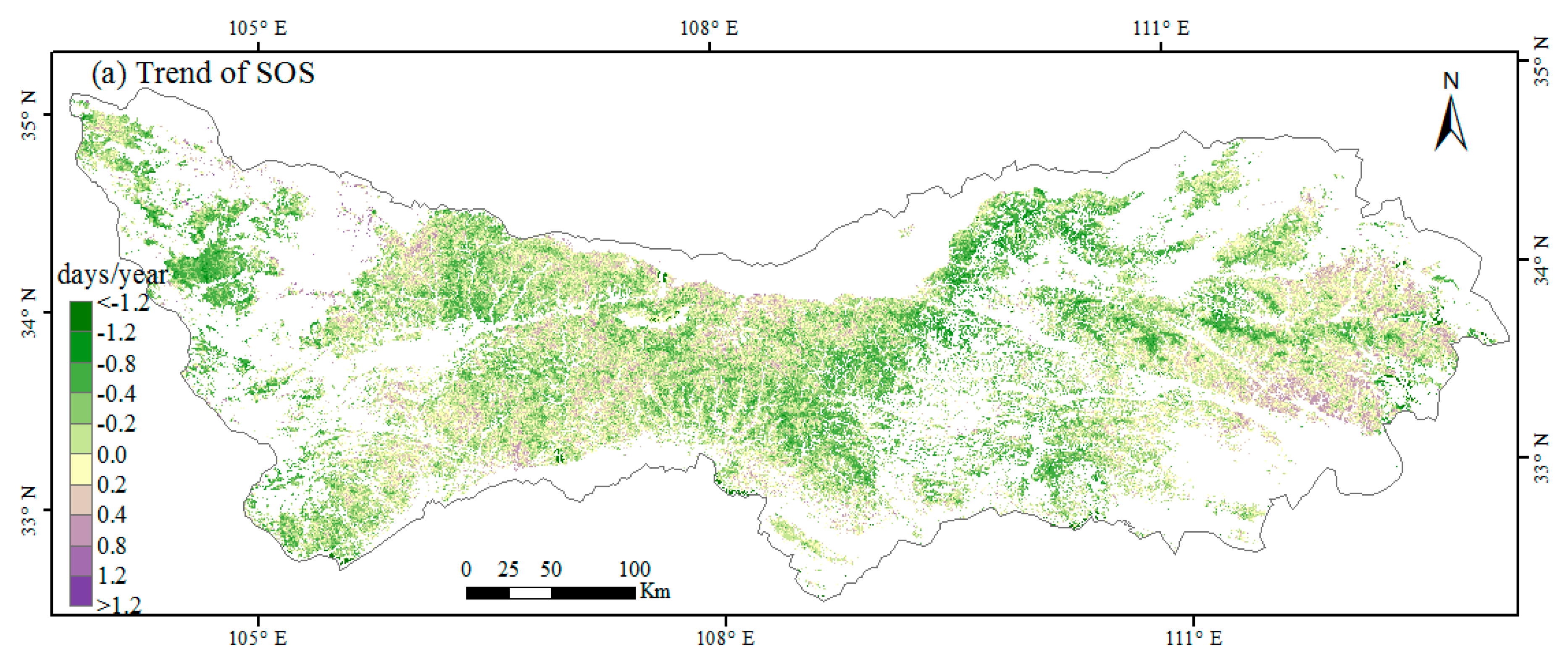
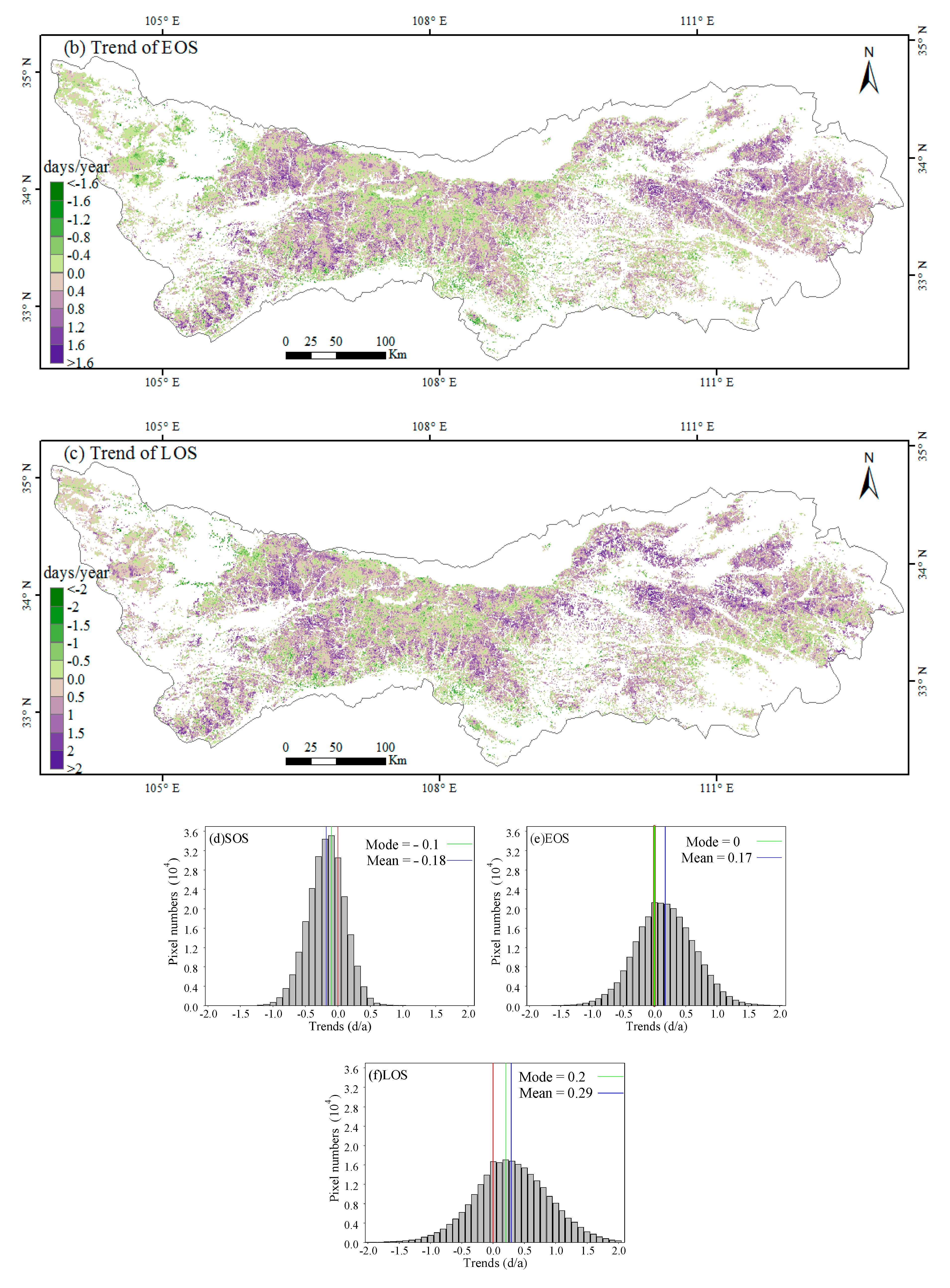
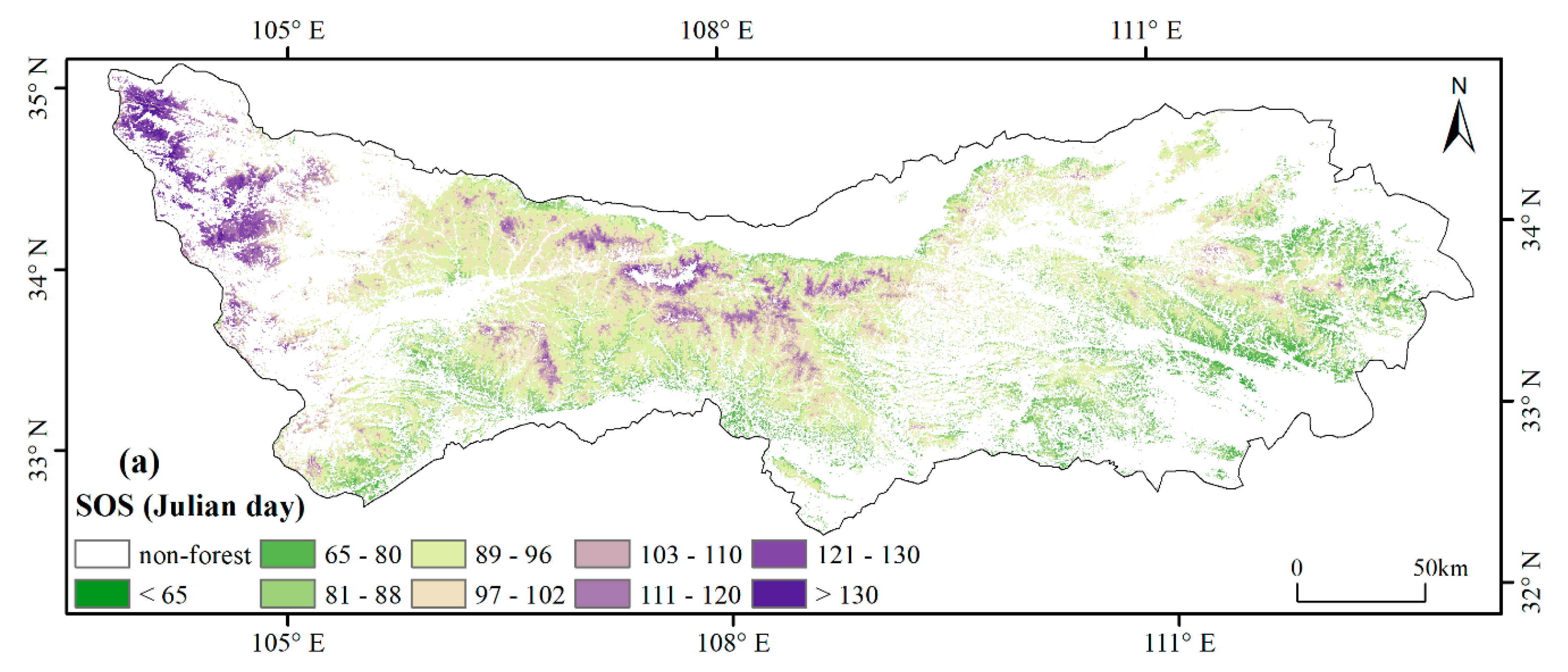
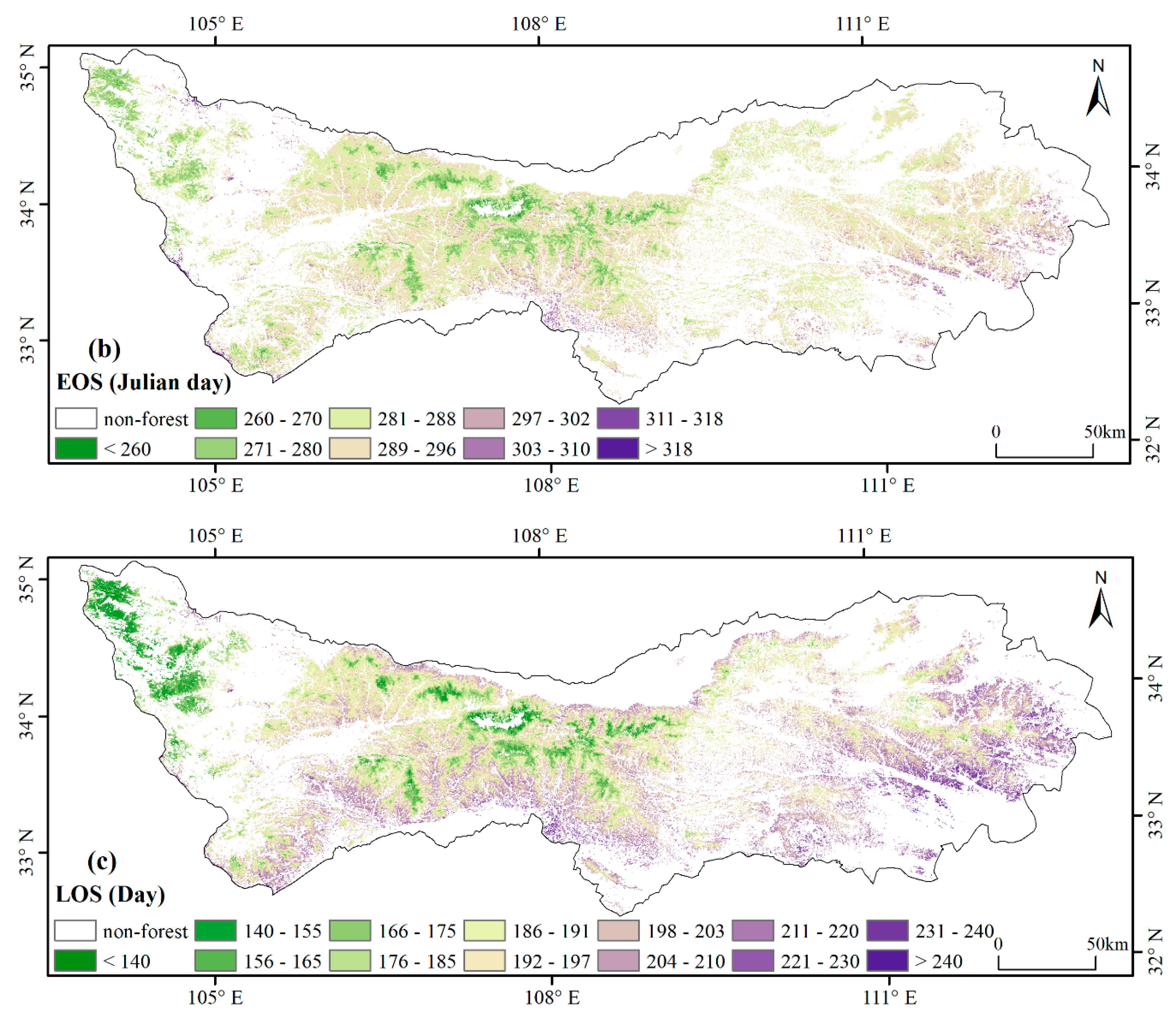
3.1. Spatial Patterns of Phenology Metrics (SOS, EOS, LOS)

The spatial patterns of the forest phenology metrics, which are averaged from multiyear phenology data from 2001 to 2017, in the QMs are shown in Figure 2. With increasing altitude, the SOS, EOS, and LOS were gradually postponed, advanced, and shortened, respectively, which was in conformance with the regional hydrothermal conditions. The SOS was generally between the 81st and 120th Julian days, using a 10% to 90% percentile (Figure 2a). Owing to the high altitudes in the west of the QMs, the SOS began later, and in the eastern part, the SOS started earlier because of the lower altitude. The central QMs have the largest elevation differences, so the span of the SOS is larger. The EOS showed the opposite trend compared with the SOS and is shown in Figure 2b. Contrary to the SOS, the EOS ends earlier in the west of the QMs because of the higher altitudes. The eastern part of the QMs has relatively lower elevations, with later EOS. The central QMs have the largest elevation differences, so the span of EOS is also larger. The dates for the EOS mainly range from the 260th to 310th Julian days, using a 10% to 90% percentile. The LOS is determined by both the SOS and the EOS. Regions with earlier SOS averaged dates and later EOS averaged dates featured longer LOS results (Figure 2c), which are usually associated with low altitudes. The LOS ranged from 150 to 230 days across the study area, using a 10% to 90% percentile.
The SOS and EOS were getting later and earlier with increasing elevation, respectively; as a consequence, the LOS became shorter with elevation (Figure 3). The SOS was delayed by 2.4 days per 100 m increase in elevation, whereas the EOS was advanced by 1.4 days, and the LOS was shortened by 3.8 days. The changes in phenology along elevation gradients were statistically significant. However, the EOS remained stable at altitudes above 2200 m above sea level (a.s.l)., and the shortening of LOS slowed down due to the stability of EOS above 2200 m a.s.l.

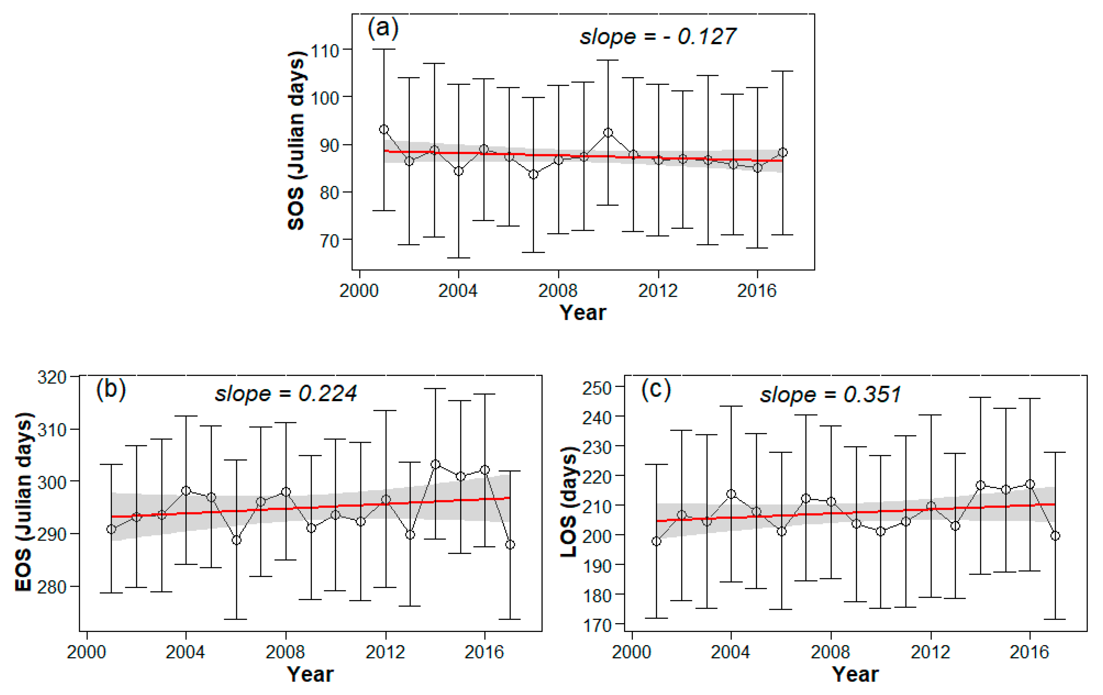
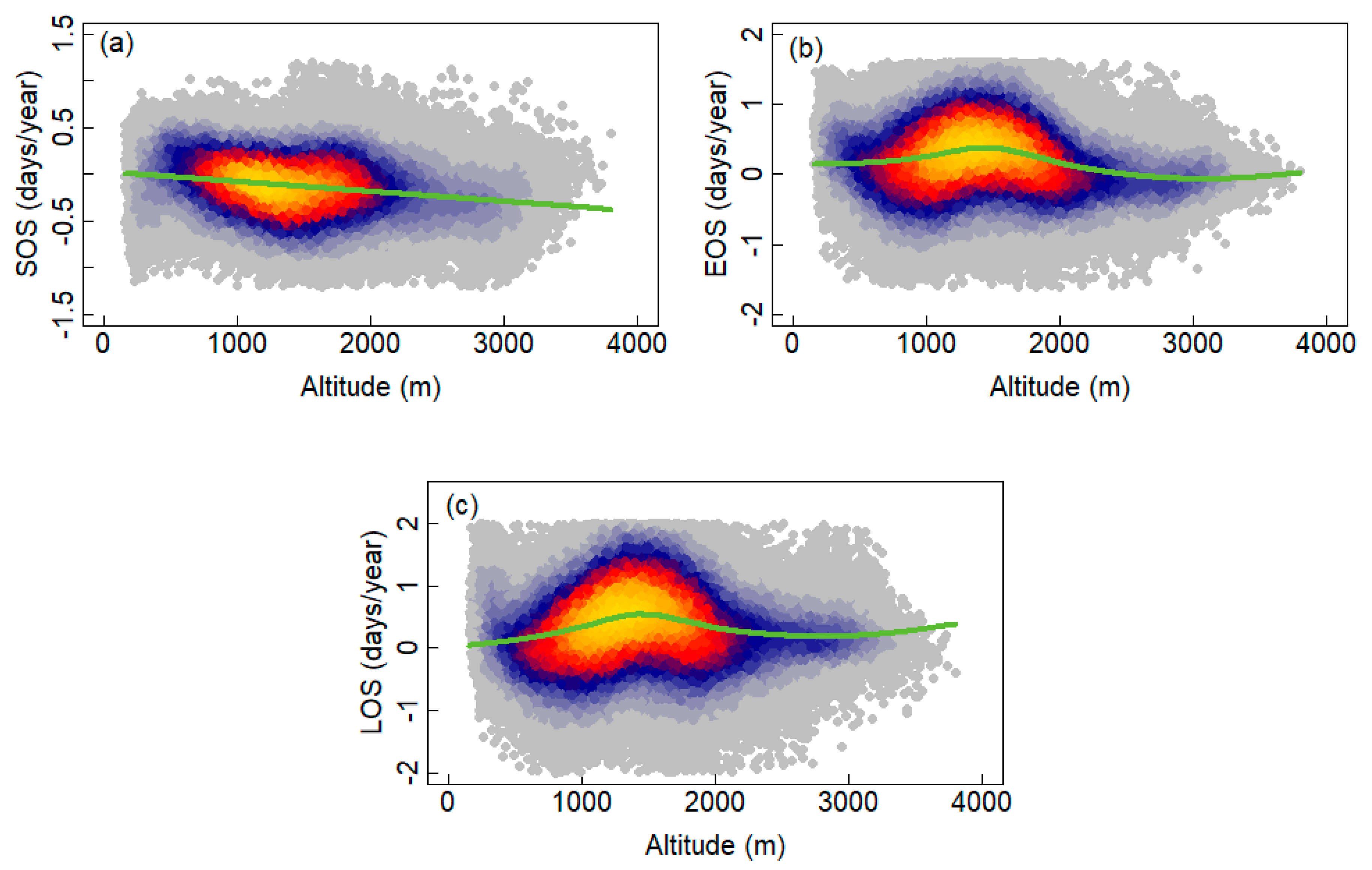
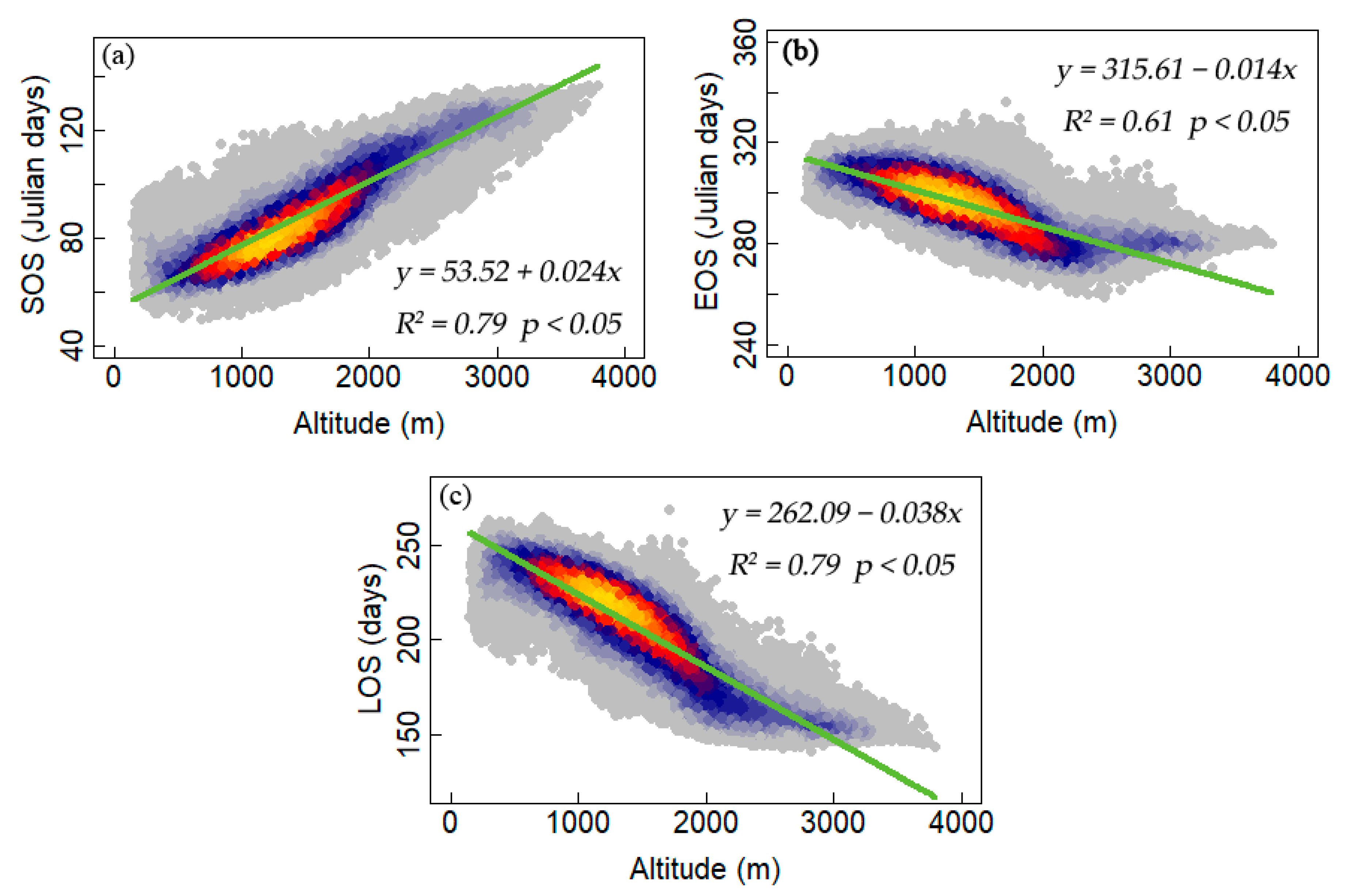
3.2. Interannual Variability and Trends of Phenology Metrics at Different Altitudes

At the regional scale, the average SOS, EOS, and LOS displayed advanced by 0.13 days year−1, delayed by 0.22 days year−1, or extended by 0.35 days year−1 from 2001 to 2017 (Figure 4). Figure 5 further illustrates the spatial distributions of the interannual variability of phenology metrics in the QMs from 2001 to 2017, which depicts a large spatial difference. The variation trend of SOS is negative 66.9% for the whole forest land in the study area and is concentrated on −0.18 days each year, denoting that most of the regions underwent an earlier SOS (Figure 5a,d). The advanced SOS is mainly located at a middle-high altitude of the QMs (Figure 5b,e). The delayed EOS is focused on 0.17 days each year, and the distribution of EOS is a flat peak. Overall, 72.2% of the entire region presented a lengthened growing season, which is caused by both the earlier SOS and later EOS (Figure 5c,f). The flatness or sharpness between the LOS and EOS is similar, and the spatial pattern of LOS is also similar to that of EOS in most of the area. According to the slopes in Figure 4, it seems EOS contributed 64% in lengthening the growing season. Therefore, a later EOS was the more significant factor in lengthening the growing season. Furthermore, we further probed how the altitude gradient influenced the differences in phenological variation and found that the inter-annual changes of SOS, EOS, and LOS showed different patterns across altitudinal gradients (Figure 6). The advanced trend in the SOS date showed a slight decrease with increasing elevation. The delayed trend in the EOS date was first increasing and then decreasing, and the peak area was about 1500 m. The changes in the trend of LOS corresponded well with the EOS.

3.3. Climate Impacts on Forest Phenology

Figure S3 shows that the spatial distribution of the lengths of the SOS and EOS preseason correspond to temperature and precipitation across altitudinal gradients. In terms of the total percentages at each month, we observed that the preseason length of SOS (EOS) to the preseason mean temperature was almost located in month 0 and 1, which is the mean temperature of the current month and the previous month for leaf-out (leaf-off) has the greatest impact of forest leaf-out and leaf-off. However, from the perspective of effects for precipitation, the preseason length of SOS and EOS are evenly distributed throughout the previous six months and have a strong relationship with the different lengths of accumulative precipitation.
The spatial patterns of the trends of preseason temperature and precipitation for SOS and EOS during 2001–2017 are shown in Figure S4. The preseason temperature for SOS shows an increasing trend in high latitudes in the middle and west of the QMs and in the west of the QMs. The preseason precipitation for SOS shows an increasing trend in the middle and west of the QMs and mainly displays a decreasing trend in the east of the QMs. The preseason temperature for EOS exhibits an increasing trend in the entire QMs, except the southwestern region. The preseason precipitation for EOS shows a non-uniform distribution and displays decreasing trends in the north and west areas.
The patterns of the partial correlation between SOS and the preseason mean temperature exhibited an inconsistent spatial distribution. Figure 7a and Table 1 show that spring SOS in the QMs were negatively correlated with temperature during Lsos across 73.2% of the QMs, and 13.2% areas, which mainly distributed in north of QMs, show significant (p < 0.05) negative correlation with the preseason mean temperature, i.e., increased spring temperature resulted in the advancement of SOS. The spatial distribution of the negative correlations between SOS and Leos-averaged temperatures mainly located in the north and east regions of QMs. Negative and positive partial correlations between preseason precipitation and SOS dominated about 60.5% and 39.5% of the QMs, and about 7.1% and 1.9% of them were significant (p < 0.05), respectively (Figure 7b, Table 1), indicating that increased precipitation resulted in the delayed of SOS, and increasing temperature and precipitation is the main factor to contribute to the advanced SOS. The positive correlations between preseason precipitation and SOS were largely sited in the middle-west high altitudes of the QMs.
On the contrary, the partial correlations for EOS mainly exhibited positive correlations with the mean temperature and showed negative correlations with accumulative precipitation during Leos (Figure 7c,d, and Table 1). A positive partial correlation between EOS and the preseason temperature during Leos dominated about 56% of the study area, which was found in middle and west of the QMs, and about 6.6% of the correlations were significant (p < 0.05), denoting that an increased temperature during Leos delayed the EOS. Meanwhile, 44% area, which was positioned in the west of the QMs, show a negative correlation with preseason temperature during Leos, and only 2.4% of the correlations were significant (p < 0.05). We also found a negative partial correlation between accumulative precipitation and EOS in 55.6% of the area, which is located in the mid-west area during Leos, and only 7.2% of the correlations were significant (p < 0.05). The 44.4% area, which is situated in the west and east of the QMs, showed a positive correlation between preseason precipitation and EOS, and only the 3.3% area was significant (p < 0.05). These results suggest that increasing temperature and precipitation have a countervailing effect on delayed EOS in the QMs.
Figure 8 shows spatial patterns of the sensitivities of the SOS (EOS) to preseason mean temperature and accumulated precipitations in the QMs during 2001–2017. The sensitivity of SOS to preseason temperature displays that an increase of 1 °C in the regionally averaged preseason temperature would advance the average SOS by 1.23 days. The 28.9% and 23.6% region shows the SOS sensitivity to preseason temperature in the north and west areas ranged from −4 to −2 days °C−1 and −2 to −1 days °C−1 (Figure 8a). Across the QMs, the sensitivity of SOS to preseason precipitation is not obvious, and an increase of 1 mm will advance 0.03 days for SOS in the regionally level. There are 57.7% of pixels that show negative precipitation sensitivity values, and the sensitivity is ranged from −0.01 to −0.15 days mm−1 in 48% of the pixels. Meanwhile, the positive sensitivity is ranged from 0 to 0.1 days mm−1 in 35% of the pixels, which occurred mostly in the high altitudes of the QMs. The sensitivity of EOS to preseason temperature shows that an increase of 1 °C in regionally an averaged preseason temperature would delay the average EOS by 0.72 days. There are about 51.3% of the pixels showed positive temperature sensitivity values, the sensitivity is mainly concentrated from 1 to 2 days °C−1 in 15.1% of the pixels and from 0 to 1 days °C−1 in 13% of the pixels, which occurred mostly in the western and middle part of the QMs. There are also 32.5% of pixels that showed negative temperature sensitivity values, and the sensitivity ranged from −2 to −4 days °C−1 in 15.8% and from −4 to −6 days °C−1 in 16.7%, which occurred mostly in the west of the QMs. Across the QMs, the sensitivity of EOS to preseason precipitation is also not obvious, and an increase of 1 mm will advance 0.002 days for EOS at the regional level. Although 52.2% of the pixels showed negative precipitation sensitivity values, which ranged mostly from 0 to −0.1 days mm−1, and the precipitation sensitivity value more than 0 days mm−1 in 47.8% of the pixels, which occurred mainly from 0 to 0.1 days mm−1.

4. Discussion

4.1. Variations in Phenology

Understanding the forest phenological changes and variation trends is valuable for reducing the negative impacts of climate change and utilizing its advantages. Recent studies have shown advanced SOS, delayed EOS, and extended LOS at middle and high latitudes of the Northern Hemisphere [10,19,20,30,32,65,66]. Zeng and Jeong et al. [20,30] also found that phenological trends became slower during 2000–2008 compared to 1982–1999 and did not display strong significance. Comparing with the changes in phenology (SOS: −7.9, EOS: 3.7; LOS: 11.6 days/decade) in China’s temperate vegetation [32] from 1982 to 1999, our results also show lower changes in phenology (SOS: −1.3, EOS: 2.2; LOS: 3.5 days/decade). Meanwhile, our results also show that the advanced magnitude of SOS is lower than the delayed magnitude of EOS, which is the opposite of what was found by Piao et al. [32]. This observation is similar to the results of Wang et al. [66], which indicates that the satellite-observed phenology change rates become slowed down during a global warming hiatus between 1998 and 2012.
The change in elevation is a key factor influencing the phenology of vegetation in mountainous environments [67,68]. Although our results indicate that elevation change was a significant factor for variations in trends of the phenological metrics, the effect was not uniform for all elevations or phenology metrics. First, the SOS was delayed by 2.4 days per 100 m with increasing altitude; the EOS was integrally advanced by 1.4 days per 100 m but stayed stagnant above 2200 m. Meanwhile, the LOS was shortened by 3.8 days per 100 m below 2200 m, and the rate of shortening became slower above 2200 m. Shen et al. [16] found a similar trend that the green-up date stayed stagnant above a certain altitude in the Qinghai-Tibetan Plateau.
Second, as for spatial distribution, the amplitude of the advanced trend for SOS slightly increased, and the amplitude of the delayed trend of EOS reached a maximum at 1500 m. Therefore, the elevation-induced advanced trend of SOS declined slightly with increasing elevation, which was illustrated by Vitasse et al. [17] and Vandvik et al. [69]. Furthermore, while previous studies only reveal an elevation-induced SOS shift [17,69], our results also show the elevation-induced EOS shift and an elevation-induced LOS shift. The declining elevation-induced phenological shift will have important implications for the structure and function of mountain ecosystems, and the actual impact of such ongoing change needs to continue to be studied in the future. In addition, the advancement and delay of SOS and EOS coexisted at different altitudes. The elevation and aspect of mountains can shift over very short distances, altering the local temperature patterns, imposing very significant impacts on the timing of phenological events, and ultimately leading to heterogeneity [16]. Ding et al. [70] showed an obvious differentiation of trends in phenological changes along the gradient. The results of Ding et al. [70] indicate that as the altitude rises, the amplitude of advancement for SOS decreases from 2.4 days year−1 to 0.3 days year−1, the amplitude of delay for EOS decreases gradually from 1.3 days year−1 to 0 days year−1, and the amplitude of lengthening for LOS decreases from 3.4 days year−1 to 0.2 days year−1. The different amplitudes of phenological change could be related to different data sources, temporal scales, and regional differences [38,59,62,70].

4.2. Relationships between Phenology Metrics and Climatic Factors

To reveal the variability of the phenology metrics (SOS, EOS, and LOS) in response to climatic factors, partial correlation analyses were carried out with preseason climatic factors (including mean temperature and cumulative precipitation). We found that a 0–2 month accumulated temperature (spring temperature), which accounted for 73.2% of the entire study area, had the greatest impact on the SOS, indicating that warming spring temperatures promoted the advancement of the SOS. This finding agrees with the results reported in the literature [32,38,62]. Zhao et al. [62] analyzed the relationship between temperature and SOS in the forest of northeast China and showed that the spring temperature had the greatest positive impact on the SOS. Tang et al. [38] also reported that the forest SOS is negatively correlated with mean spring temperature in the Greater Khingan Mountain area. Crabbe et al. [71] showed that warmer spring temperatures at high latitudes in Europe lead to a significantly earlier SOS in broad-leaf deciduous forest and mixed forest. Our study found that the duration, in months, of temperatures correlated with EOS increased with altitude. Growing degree days have a negative correlation with chilling accumulation [12]. Therefore, a longer duration of cooling, in days, is required at high altitudes to initiate a delayed EOS. This finding is consistent with other studies [71,72,73]. Crabbe et al. [71] showed that warmer temperatures in extreme warm autumn events lead to significantly delayed EOS for needle leaf evergreen forest, broad-leaf deciduous forests, and mixed forests. We also showed that the cumulative precipitation in different months affected the EOS for the forests. Some studies have indicated that LOS has been prolonged in recent years, a change that is more closely associated with temperature than with precipitation, and that the different patterns between the phenological metrics and climate factors may be associated with their growth environment [74]. Several studies have also proposed that a time-lagged and cumulative effect exists between vegetation growth and climate changes [32,75,76,77]. Different lagged and cumulated effects between the phenological metrics and climate factors have been noticed and attributed to species, and locations, at diverse temporal and spatial scales [22]. Chmielewski and Rotzer [78] found a significant negative relationship between the SOS and the mean temperature of spring (February–April). Piao et al. [32] identified that the phenological metrics were correlated most significantly with the mean temperature during the previous 2–4 months. Our results indicated that the absolute value of the correlation coefficient between the SOS and temperature was higher in the preceding two months before SOS, implying that the cumulative temperature during the two months before the SOS contributed significantly to the growth of forests. A similar pattern can also be observed for the relationship between temperature and the EOS. The temperature of the preceding two months before the EOS contributed significantly to the growth of forests. Regional differences in temperature sensitivity may be derived from interactions among climatic factors [60]. Previous studies indicate that temperature sensitivity can vary in space and time [13,79]. Our result showed that the mean sensitivity of SOS to preseason temperature is −1.23 days °C−1, which is lower than the temperate region (−2.5 days °C−1) [79]. Symmetric effects of daytime and nighttime warming also have different sensitivity to phenology metrics, for example, an increase of 1 °C Tmin and Tmax in spring would advance SOS 1.34 days and 0.64 days, respectively [80]. In contrast to the extensive research efforts on the sensitivity of SOS, the sensitivity of EOS to temperature is more challenging to understand [22,81]. Although there are about 0.72 days delay with 1 °C increasing, our result showed a different sensitivity of EOS preseason temperature between the eastern and mid-west area. Precipitation has no obvious effects on SOS or EOS at the regional level. A significant interaction between temperature and precipitation indicates the complex mechanisms of phenological responses to climate change [82].

4.3. Uncertainty and Future Research Needs

Our results showed that the average SOS was mainly distributed between the 81th and 120th Julian days, and the mean EOS was primarily between the 260th and 310th Julian days, which was in line with the results of previous studies [26,65]. According to the phenology statistics of eight representative woody plants, including Princess tree (Paulownia tomentosa), Babylon weeping willow (Salix babylonica), Dwarf elm (Ulmus pumila), Paper mulberry (Broussonetia papyrifera), Chinese wild peach (Prunus davidiana), and Black locust (Robinia pseudoacacia) in the northern edge of the Qingling Mountains, from 1998 to 2008, He [83] showed that the leaves were completely unfolded on the 96.5th Julian day of the year, and the total discoloration of the leaves was on the 308.8th Julian day of the same year. Li and Liu [84] conducted a statistical survey based on phenological observations from 1986 to 2010 at Xi’an Botanical Garden and Qujiang Scenic Spot. Their results indicated that 37.7% of the plants started leaf-out in March, 61.6% of the plants started leaf-out in April, 67.6% of the plants began to color and defoliate in September, while 32.4% of the plants discolored in October. These conclusions are consistent with the result of our study that 94.2% of trees’ SOS in the QMs occurred between the 81th and 120th Julian days, and 98% of trees’ EOS appeared between the 270th and 311th Julian days. The spatial extent and time span shown by Wang, Xue, Quan and He [53] is almost consistent; therefore, the spatial distribution of the SOS and EOS showed a similar pattern with our results. Our study demonstrated that using a MODIS EVI time-series dataset to obtain the phenological metrics offered acceptable reliability, and the results were comparable with the ground observation data and can be used to reveal the forest phenological characteristics.
Differences in the models for smoothing the vegetation index and the model parameters resulted in potential differences of uncertainty and bias among alternative phenology analyses [85]. Even with the same model, different thresholds often lead to changes in phenology metrics. The uncertainty of our research results is firstly associated with the reconstruction of remote sensing data by the HANTS algorithm. When the time-series dataset is reconstructed, the acquired images are not as time-critical as the Fast Fourier Transform (FFT) with equal time interval images. Differences in the time intervals of time-series images and in the calibrations of model parameters affect the amounts or degrees of uncertainty and bias in the results [38,86]. Therefore, ground-based phenological observations should be incorporated into the threshold of phenological estimates to improve the accuracy of phenological estimates in the future. This research expanded to an in-depth investigation of the variation in phenological response to climate change. Phenology changes are strongly influenced by a combination of climate factors such as temperature, precipitation, and solar radiation, which typically are significantly correlated with elevation.
The shortening of the growing season at low altitudes of the QMs may be related to mixed pixels containing both forests and cultivated vegetation. This is because the cultivated vegetation in the QMs is mainly planted in lowlands with gentle slopes and in reclamation zones of the low valley with altitudes between 984 m a.s.l. and 1375 m a.s.l. [87]. The increases in temperature and heat resources to the north of the QMs were found to be larger than those in the south [88]. It was also found that in recent years, the boundaries between the semi-arid and humid areas, and between the warm temperate zone and the subtropical zone, have shifted northward [89]. The question of how to quantify the differentiated impact of climatic factors such as temperature, precipitation, and sunshine duration on the phenology of the north side and south side of the QMs should be addressed independently in the follow-up studies.

5. Conclusions

Based on the time series of the MODIS EVI dataset with 8-day and 500 m resolutions and climate dataset, we estimated pixel-based SOS, EOS, and LOS and analyzed phenological change across altitudinal gradients and the influence of the preseason temperature and precipitation across the QMs in Central China, for the period 2001–2017. The results indicated that the SOS was more sensitive to changes in elevations than the EOS. The SOS, EOS, and LOS were delayed, advanced, and shortened by 2.4, 1.4, and 3.8 days per every 100 m increase in altitude, respectively. The EOS was found to be the most significant factor in prolonging the growing season. The elevation-induced leaf-out shift declined slightly from 2001 to 2017. The derived partial correlation coefficients between the phenological metrics and the climatic factors indicated that the current and previous-month mean temperature had strong impacts on SOS and EOS. Furthermore, the temperature was significantly correlated with variations in SOS and EOS, an increase of 1 °C in the regionally averaged preseason temperature would advance the average SOS by 1.23 days and delay the average EOS by 0.72 days. The precipitation was observed to have no significant correlation with SOS and EOS, the sensitivity of SOS and EOS to the preseason precipitation was not obvious across the QMs. This study provides valuable evidence to improve our understanding of the complex impacts of climatic and elevational changes on the spatiotemporal phenology variabilities and trends in the QMs, an important ecotone in China. Future studies are still needed to investigate the phenology response of different species and boundary effects in the QMs.

Supplementary Materials

The following are available online at https://0-www-mdpi-com.brum.beds.ac.uk/1999-4907/10/11/1007/s1, Figure S1: An example of the determination of the start (end) of the growing season using MODIS EVI with SOS (EOS) extraction method. Figure S2: The threshold values were determined according to the lowest absolute error between the leaf-out and leaf senescence dates measured in situ. Figure S3: The length of the preseason period corresponds to temperature and precipitation. Figure S4: Change trend of the preseason temperature and precipitation for SOS and EOS.

Author Contributions

H.X. and Y.Q. conceived and designed the experiments; H.X. performed programming work, analysis, discussions, and wrote most sections of the manuscript. Y.Q., G.F., Y.C., H.S., Y.O., Q.M., and G.L. supplied suggestions and comments for the manuscript. All authors reviewed and revised the manuscript.

Funding

This research was funded jointly by the program for key scientific research in the University of Henan Province (18A170002), and the National Natural Science Foundation Project of China (41701503, 41601091,41701433 and 41701186). We are grateful to all contractors, image providers, and the anonymous reviewers for their valuable comments and suggestions.

Conflicts of Interest

The authors declare no conflict of interest.

References

  1. Lieth, H. Purposes of A Phenology Book; Springer: Berlin, Germany, 1974. [Google Scholar]
  2. Fu, Y.H.; Piao, S.; Zhou, X.; Geng, X.; Hao, F.; Vitasse, Y.; Janssens, I.A. Short photoperiod reduces the temperature sensitivity of leaf-out in saplings of Fagus sylvatica but not in Horse chestnut. Glob. Chang. Biol. 2019, 25, 1696–1703. [Google Scholar] [CrossRef] [PubMed]
  3. Chuine, I. Why does phenology drive species distribution? Philos. Trans. R. Soc. B Biol. Sci. 2010, 365, 3149–3160. [Google Scholar] [CrossRef] [PubMed]
  4. Memmott, J.; Craze, P.G.; Waser, N.M.; Price, M.V. Global warming and the disruption of plant–pollinator interactions. Ecol. Lett. 2007, 10, 710–717. [Google Scholar] [CrossRef] [PubMed]
  5. Cleland, E.E.; Chuine, I.; Menzel, A.; Mooney, H.A.; Schwartz, M.D. Shifting plant phenology in response to global change. Trends Ecol. Evol. 2007, 22, 357–365. [Google Scholar] [CrossRef] [PubMed]
  6. Piao, S.; Ciais, P.; Friedlingstein, P.; Peylin, P.; Reichstein, M.; Luyssaert, S.; Margolis, H.; Fang, J.; Barr, A.; Chen, A. Net carbon dioxide losses of northern ecosystems in response to autumn warming. Nature 2008, 451, 49–52. [Google Scholar] [CrossRef] [PubMed]
  7. Jeong, S.J.; Medvigy, D.; Shevliakova, E.; Malyshev, S. Uncertainties in terrestrial carbon budgets related to spring phenology. J. Geophys. Res. Biogeosci. 2012, 117. [Google Scholar] [CrossRef]
  8. Piao, S.; Friedlingstein, P.; Ciais, P.; Viovy, N.; Demarty, J. Growing season extension and its impact on terrestrial carbon cycle in the Northern Hemisphere over the past 2 decades. Glob. Biogeochem. Cycles 2007, 21, 1148–1154. [Google Scholar] [CrossRef]
  9. Peñuelas, J.; Filella, I. Phenology feedbacks on climate change. Science 2009, 324, 887–888. [Google Scholar] [CrossRef] [PubMed]
  10. Myneni, R.B.; Keeling, C.D.; Tucker, C.J.; Asrar, G.; Nemani, R.R. Increased plant growth in the northern high latitudes from 1981 to 1991. Nature 1997, 386, 698–702. [Google Scholar] [CrossRef]
  11. Fu, Y.H.; Piao, S.; Vitasse, Y.; Zhao, H.; de Boeck, H.J.; Liu, Q.; Yang, H.; Weber, U.; Hänninen, H.; Janssens, I.A. Increased heat requirement for leaf flushing in temperate woody species over 1980–2012: Effects of chilling, precipitation and insolation. Glob. Chang. Biol. 2015, 21, 2687–2697. [Google Scholar] [CrossRef] [PubMed]
  12. Fu, Y.H.; Piao, S.; Zhao, H.; Jeong, S.J.; Wang, X.; Vitasse, Y.; Ciais, P.; Janssens, I.A. Unexpected role of winter precipitation in determining heat requirement for spring vegetation green-up at northern middle and high latitudes. Glob. Chang. Biol. 2014, 20, 3743–3755. [Google Scholar] [CrossRef] [PubMed]
  13. Fu, Y.H.; Zhao, H.; Piao, S.; Peaucelle, M.; Peng, S.; Zhou, G.; Ciais, P.; Huang, M.; Menzel, A.; Peñuelas, J. Declining global warming effects on the phenology of spring leaf unfolding. Nature 2015, 526, 104. [Google Scholar] [CrossRef] [PubMed]
  14. Nicolas, D.; Ghislain, P.; Thuy, L.E.T.; Laurent, K.; Shaun, Q.; Ian, W.; Dennis, D.; Violetta, F. Spring phenology in boreal Eurasia over a nearly century time scale. Glob. Chang. Biol. 2008, 14, 603–614. [Google Scholar]
  15. Piao, S.; Tan, J.; Chen, A.; Fu, Y.H.; Ciais, P.; Liu, Q.; Janssens, I.A.; Vicca, S.; Zeng, Z.; Jeong, S.J. Leaf onset in the northern hemisphere triggered by daytime temperature. Nat. Commun. 2015, 6, 6911. [Google Scholar] [CrossRef] [PubMed]
  16. Shen, M.; Zhang, G.; Cong, N.; Wang, S.; Kong, W.; Piao, S. Increasing altitudinal gradient of spring vegetation phenology during the last decade on the Qinghai–Tibetan Plateau. Agric. For. Meteorol. 2014, 189, 71–80. [Google Scholar] [CrossRef]
  17. Vitasse, Y.; Signarbieux, C.; Fu, Y.H. Global warming leads to more uniform spring phenology across elevations. Proc. Natl. Acad. Sci. USA 2018, 115, 1004–1008. [Google Scholar] [CrossRef] [PubMed]
  18. Fu, Y.H.; Piao, S.; de Beeck, M.O.; Cong, N.; Zhao, H.; Zhang, Y.; Menzel, A.; Janssens, I.A. Recent spring phenology shifts in western Central Europe based on multiscale observations. Glob. Ecol. Biogeogr. 2014, 23, 1255–1263. [Google Scholar] [CrossRef]
  19. Wang, X.; Piao, S.; Xu, X.; Ciais, P.; MacBean, N.; Myneni, R.B.; Li, L. Has the advancing onset of spring vegetation green-up slowed down or changed abruptly over the last three decades? Glob. Ecol. Biogeogr. 2015, 24, 621–631. [Google Scholar] [CrossRef]
  20. Jeong, S.J.; Chang-Hoi, H.O.; Gim, H.J.; Brown, M.E. Phenology shifts at start vs. end of growing season in temperate vegetation over the Northern Hemisphere for the period 1982–2008. Glob. Chang. Biol. 2011, 17, 2385–2399. [Google Scholar] [CrossRef]
  21. Wu, C.; Wang, X.; Wang, H.; Ciais, P.; Peñuelas, J.; Myneni, R.B.; Desai, A.R.; Gough, C.M.; Gonsamo, A.; Black, A.T. Contrasting responses of autumn-leaf senescence to daytime and night-time warming. Nat. Clim. Chang. 2018, 8, 1092. [Google Scholar] [CrossRef]
  22. Walther, G.-R.; Post, E.; Convey, P.; Menzel, A.; Parmesan, C.; Beebee, T.J.; Fromentin, J.-M.; Hoegh-Guldberg, O.; Bairlein, F. Ecological responses to recent climate change. Nature 2002, 416, 389. [Google Scholar] [CrossRef] [PubMed]
  23. Killingbeck, K.T. Nutrients in senesced leaves: Keys to the search for potential resorption and resorption proficiency. Ecology 1996, 77, 1716–1727. [Google Scholar] [CrossRef]
  24. Maillard, A.; Diquélou, S.; Billard, V.; Laîné, P.; Garnica, M.; Prudent, M.; Garcia-Mina, J.-M.; Yvin, J.-C.; Ourry, A. Leaf mineral nutrient remobilization during leaf senescence and modulation by nutrient deficiency. Front. Plant Sci. 2015, 6, 317. [Google Scholar] [CrossRef] [PubMed]
  25. Wu, C.; Chen, J.M.; Black, T.A.; Price, D.T.; Kurz, W.A.; Desai, A.R.; Gonsamo, A.; Jassal, R.S.; Gough, C.M.; Bohrer, G. Interannual variability of net ecosystem productivity in forests is explained by carbon flux phenology in autumn. Glob. Ecol. Biogeogr. 2013, 22, 994–1006. [Google Scholar] [CrossRef]
  26. Richardson, A.D.; Black, T.A.; Ciais, P.; Delbart, N.; Friedl, M.A.; Gobron, N.; Hollinger, D.Y.; Kutsch, W.L.; Longdoz, B.; Luyssaert, S. Influence of spring and autumn phenological transitions on forest ecosystem productivity. Philos. Trans. R. Soc. B 2010, 365, 3227–3246. [Google Scholar] [CrossRef] [PubMed]
  27. Fu, Y.H.; Piao, S.; Delpierre, N.; Hao, F.; Hänninen, H.; Liu, Y.; Sun, W.; Janssens, I.A.; Campioli, M. Larger temperature response of autumn leaf senescence than spring leaf-out phenology. Glob. Chang. Biol. 2018, 24, 2159–2168. [Google Scholar] [CrossRef] [PubMed]
  28. Marchin, R.M.; Salk, C.F.; Hoffmann, W.A.; Dunn, R.R. Temperature alone does not explain phenological variation of diverse temperate plants under experimental warming. Glob. Chang. Biol. 2015, 21, 3138–3151. [Google Scholar] [CrossRef] [PubMed]
  29. Zhao, J.; Zhang, H.; Zhang, Z.; Guo, X.; Li, X.; Chen, C. Spatial and Temporal Changes in Vegetation Phenology at Middle and High Latitudes of the Northern Hemisphere over the Past Three Decades. Remote Sens. 2015, 7, 10973–10995. [Google Scholar] [CrossRef]
  30. Zeng, H.; Jia, G.; Epstein, H. Recent changes in phenology over the northern high latitudes detected from multi-satellite data. Environ. Res. Lett. 2011, 6, 45508–45518. [Google Scholar] [CrossRef]
  31. Liu, Q.; Fu, Y.H.; Zeng, Z.; Huang, M.; Li, X.; Piao, S. Temperature, precipitation, and insolation effects on autumn vegetation phenology in temperate China. Glob. Chang. Biol. 2016, 22, 644–655. [Google Scholar] [CrossRef] [PubMed]
  32. Piao, S.; Fang, J.; Zhou, L.; Ciais, P.; Zhu, B. Variations in satellite-derived phenology in China′s temperate vegetation. Glob. Chang. Biol. 2006, 12, 672–685. [Google Scholar] [CrossRef]
  33. Shen, M.; Piao, S.; Cong, N.; Zhang, G.; Jassens, I.A. Precipitation impacts on vegetation spring phenology on the Tibetan Plateau. Glob. Chang. Biol. 2015, 21, 3647–3656. [Google Scholar] [CrossRef] [PubMed] [Green Version]
  34. Fu, Y.; He, H.; Zhao, J.; Larsen, D.; Zhang, H.; Sunde, M.; Duan, S. Climate and Spring Phenology Effects on Autumn Phenology in the Greater Khingan Mountains, Northeastern China. Remote Sens. 2018, 10, 449. [Google Scholar] [CrossRef] [Green Version]
  35. Zhao, W.; Li, A. A review on land surface processes modelling over complex terrain. Adv. Meteorol. 2015, 17. [Google Scholar] [CrossRef] [Green Version]
  36. Pepin, N.; Bradley, R.; Diaz, H.; Baraër, M.; Caceres, E.; Forsythe, N.; Fowler, H.; Greenwood, G.; Hashmi, M.; Liu, X. Elevation-dependent warming in mountain regions of the world. Nat. Clim. Chang. 2015, 5, 424. [Google Scholar]
  37. Lucht, W.; Prentice, I.C.; Myneni, R.B.; Sitch, S.; Friedlingstein, P.; Cramer, W.; Bousquet, P.; Buermann, W.; Smith, B. Climatic control of the high-latitude vegetation greening trend and Pinatubo effect. Science 2002, 296, 1687–1689. [Google Scholar] [CrossRef] [PubMed] [Green Version]
  38. Tang, H.; Li, Z.; Zhu, Z.; Chen, B.; Zhang, B.; Xin, X. Variability and climate change trend in vegetation phenology of recent decades in the Greater Khingan Mountain area, Northeastern China. Remote Sens. 2015, 7, 11914–11932. [Google Scholar] [CrossRef] [Green Version]
  39. Zhou, L.; He, H.; Sun, X.; Zhang, L.; Yu, G.; Ren, X.; Wang, J.; Junhui, Z. Species- and Community-Scale Simulation of the Phenology of a Temperate Forest in Changbai Mountain Based on Digital Camera Images. J. Resour. Ecol. 2012, 4, 317–326. [Google Scholar]
  40. van Leeuwen, W.; Hartfield, K.; Miranda, M.; Meza, F. Trends and ENSO/AAO Driven Variability in NDVI Derived Productivity and Phenology alongside the Andes Mountains. Remote Sens. 2013, 5, 1177–1203. [Google Scholar] [CrossRef] [Green Version]
  41. He, Z.; Du, J.; Zhao, W.; Yang, J.; Chen, L.; Zhu, X.; Chang, X.; Liu, H. Assessing temperature sensitivity of subalpine shrub phenology in semi-arid mountain regions of China. Agric. For. Meteorol. 2015, 213, 42–52. [Google Scholar] [CrossRef]
  42. Zhang, X.; Friedl, M.A.; Schaaf, C.B.; Strahler, A.H.; Hodges, J.C.; Gao, F.; Reed, B.C.; Huete, A. Monitoring vegetation phenology using MODIS. Remote Sens. Environ. 2003, 84, 471–475. [Google Scholar] [CrossRef]
  43. Zhang, X.; Wang, J.; Gao, F.; Liu, Y.; Schaaf, C.; Friedl, M.; Yu, Y.; Jayavelu, S.; Gray, J.; Liu, L. Exploration of scaling effects on coarse resolution land surface phenology. Remote Sens. Environ. 2017, 190, 318–330. [Google Scholar] [CrossRef] [Green Version]
  44. Fisher, J.I.; Mustard, J.F.; Vadeboncoeur, M.A. Green leaf phenology at Landsat resolution: Scaling from the field to the satellite. Remote Sens. Environ. 2006, 100, 265–279. [Google Scholar] [CrossRef]
  45. Pan, Z.; Huang, J.; Zhou, Q.; Wang, L.; Cheng, Y.; Zhang, H.; Blackburn, G.A.; Yan, J.; Liu, J. Mapping crop phenology using NDVI time-series derived from HJ-1 A/B data. Int. J. Appl. Earth Observ. Geoinf. 2015, 34, 188–197. [Google Scholar] [CrossRef] [Green Version]
  46. Vrieling, A.; Meroni, M.; Darvishzadeh, R.; Skidmore, A.K.; Wang, T.; Zurita-Milla, R.; Oosterbeek, K.; O′Connor, B.; Paganini, M. Vegetation phenology from Sentinel-2 and field cameras for a Dutch barrier island. Remote Sens. Environ. 2018, 215, 517–529. [Google Scholar] [CrossRef]
  47. Piao, S.; Liu, Q.; Chen, A.; Janssens, I.A.; Fu, Y.; Dai, J.; Liu, L.; Lian, X.; Shen, M.; Zhu, X. Plant phenology and global climate change: Current progresses and challenges. Glob. Chang. Biol. 2019, 25, 1922–1940. [Google Scholar] [CrossRef] [PubMed]
  48. Zhao, W.; Li, A.; Jin, H.; Zhang, Z.; Bian, J.; Yin, G. Performance Evaluation of the Triangle-Based Empirical Soil Moisture Relationship Models Based on Landsat-5 TM Data and In Situ Measurements. IEEE Trans. Geosci. Remote Sens. 2017, 55, 2632–2645. [Google Scholar] [CrossRef]
  49. Xia, H.; Li, A.; Feng, G.; Li, Y.; Qin, Y.; Lei, G.; Cui, Y. The Effects of Asymmetric Diurnal Warming on Vegetation Growth of the Tibetan Plateau over the Past Three Decades. Sustainability 2018, 10, 1103. [Google Scholar] [CrossRef] [Green Version]
  50. Xia, H.; Zhao, W.; Li, A.; Bian, J.; Zhang, Z. Subpixel Inundation Mapping Using Landsat-8 OLI and UAV Data for a Wetland Region on the Zoige Plateau, China. Remote Sens. 2017, 9, 31. [Google Scholar] [CrossRef] [Green Version]
  51. Huete, A.; Didan, K.; Miura, T.; Rodriguez, E.P.; Gao, X.; Ferreira, L.G. Overview of the radiometric and biophysical performance of the MODIS vegetation indices. Remote Sens. Environ. 2002, 83, 195–213. [Google Scholar] [CrossRef]
  52. Xia, H.; Li, A.; Zhao, W.; Bian, J.; Lei, G. Spatiotemporal variations of forest phenology in the Qinling zone based on remote sensing monitoring. Prog. Geogr. 2015, 34, 1297–1305. [Google Scholar]
  53. Wang, Z.; Xue, C.; Quan, W.; He, H. Spatiotemporal variations of forest phenology in the Qinling Mountains and its response to a critical temperature of 10 °C. J. Appl. Remote Sens. 2018, 12, 022202. [Google Scholar] [CrossRef] [Green Version]
  54. The USGS EROS Data Center. Available online: http:/eros.usgs.gov/ (accessed on 2 August 2016).
  55. Hutchinson, M.F.; Xu, T. Anusplin Version 4.2 User Guide; Centre for Resource and Environmental Studies, The Australian National University: Canberra, Australia, 2004; Volume 54. [Google Scholar]
  56. Brovelli, M.; Molinari, M.; Hussein, E.; Chen, J.; Li, R. The first comprehensive accuracy assessment of GlobeLand30 at a national level: Methodology and results. Remote Sens. 2015, 7, 4191–4212. [Google Scholar] [CrossRef] [Green Version]
  57. Chen, J.; Cao, X.; Peng, S.; Ren, H. Analysis and applications of GlobeLand30: A review. ISPRS Int. J. Geoinf. 2017, 6, 230. [Google Scholar] [CrossRef] [Green Version]
  58. Zhou, J.; Jia, L.; Menenti, M. Reconstruction of global MODIS NDVI time series: Performance of Harmonic ANalysis of Time Series (HANTS). Remote Sens. Environ. 2015, 163, 217–228. [Google Scholar] [CrossRef]
  59. Roerink, G.J.; Menenti, M.; Verhoef, W. Reconstructing cloudfree NDVI composites using Fourier analysis of time series. Int. J. Remote Sens. 2000, 21, 1911–1917. [Google Scholar] [CrossRef]
  60. Cong, N.; Wang, T.; Nan, H.; Ma, Y.; Wang, X.; Myneni, R.B.; Piao, S. Changes in satellite-derived spring vegetation green-up date and its linkage to climate in China from 1982 to 2010: A multimethod analysis. Glob. Chang. Biol. 2013, 19, 881–891. [Google Scholar] [CrossRef] [PubMed]
  61. White, M.A.; Beurs, D.; Kirsten, M.; Didan, K.; Inouye, D.W.; Richardson, A.D.; Jensen, O.P.; O′keefe, J.; Zhang, G.; Nemani, R.R. Intercomparison, interpretation, and assessment of spring phenology in North America estimated from remote sensing for 1982–2006. Glob. Chang. Biol. 2009, 15, 2335–2359. [Google Scholar] [CrossRef]
  62. Zhao, J.; Wang, Y.; Zhang, Z.; Zhang, H.; Guo, X.; Yu, S.; Du, W.; Huang, F. The Variations of Land Surface Phenology in Northeast China and Its Responses to Climate Change from 1982 to 2013. Remote Sens. 2016, 8, 400. [Google Scholar] [CrossRef] [Green Version]
  63. Liu, Q.; Fu, Y.H.; Zhu, Z.; Liu, Y.; Liu, Z.; Huang, M.; Janssens, I.A.; Piao, S. Delayed autumn phenology in the Northern Hemisphere is related to change in both climate and spring phenology. Glob. Chang. Biol. 2016, 22, 3702–3711. [Google Scholar] [CrossRef] [PubMed]
  64. Ma, L.; Xia, H.; Meng, Q. Spatiotemporal Variability of Asymmetric Daytime and Night-Time Warming and Its Effects on Vegetation in the Yellow River Basin from 1982 to 2015. Sensors 2019, 19, 1832. [Google Scholar] [CrossRef] [PubMed] [Green Version]
  65. Zhou, L.; Tucker, C.J.; Kaufmann, R.K.; Slayback, D.; Shabanov, N.V.; Myneni, R.B. Variations in northern vegetation activity inferred from satellite data of vegetation index during 1981 to 1999. J. Geophys. Res. Atmos. 2001, 106, 20069–20083. [Google Scholar] [CrossRef]
  66. Wang, X.; Xiao, J.; Li, X.; Cheng, G.; Ma, M.; Zhu, G.; Arain, M.A.; Black, T.A.; Jassal, R.S. No trends in spring and autumn phenology during the global warming hiatus. Nat. Commun. 2019, 10, 2389. [Google Scholar] [CrossRef] [PubMed]
  67. Colombo, R.; Busetto, L.; Migliavacca, M.; Cremonese, E.; Meroni, M.; Galvagno, M.; Rossini, M.; Siniscalco, C.; Cella, U.M.D. On the spatial and temporal variability of Larch phenological cycle in mountainous areas. Eur. J. Remote Sens. 2009, 41, 79–96. [Google Scholar] [CrossRef]
  68. Dunn, A.H.; Beurs, K.M.D. Land surface phenology of North American mountain environments using moderate resolution imaging spectroradiometer data. Remote Sens. Environ. 2011, 115, 1220–1233. [Google Scholar] [CrossRef]
  69. Vandvik, V.; Halbritter, A.H.; Telford, R.J. Greening up the mountain. Proc. Natl. Acad. Sci. USA 2018, 115, 833–835. [Google Scholar] [CrossRef] [PubMed] [Green Version]
  70. Ding, M.; Zhang, Y.; Sun, X.; Liu, L.; Wang, Z.; Bai, W. Spatiotemporal variation in alpine grassland phenology in the Qinghai-Tibetan Plateau from 1999 to 2009. Chin. Sci. Bull. 2013, 58, 396–405. [Google Scholar] [CrossRef] [Green Version]
  71. Crabbe, R.A.; Dash, J.; Rodriguez-Galiano, V.F.; Janous, D.; Pavelka, M.; Marek, M.V. Extreme warm temperatures alter forest phenology and productivity in Europe. Sci. Total Environ. 2016, 563, 486–495. [Google Scholar] [CrossRef] [PubMed]
  72. Ge, Q.; Dai, J.; Cui, H.; Wang, H. Spatiotemporal Variability in Start and End of Growing Season in China Related to Climate Variability. Remote Sens. 2016, 8, 433. [Google Scholar] [CrossRef] [Green Version]
  73. Yang, Y.; Guan, H.; Shen, M.; Liang, W.; Jiang, L. Changes in autumn vegetation dormancy onset date and the climate controls across temperate ecosystems in China from 1982 to 2010. Glob. Chang. Biol. 2015, 21, 652–665. [Google Scholar] [CrossRef] [PubMed]
  74. Moulin, S.; Kergoat, L.; Viovy, N.; Dedieu, G. Global-scale assessment of vegetation phenology using NOAA/AVHRR satellite measurements. J. Clim. 1997, 10, 1154–1170. [Google Scholar] [CrossRef]
  75. Zhou, L.; Kaufmann, R.K.; Tian, Y.; Myneni, R.B.; Tucker, C.J. Relation between interannual variations in satellite measures of northern forest greenness and climate between 1982 and 1999. J. Geophys. Res. Atmos. 2003, 108, 4004. [Google Scholar] [CrossRef] [Green Version]
  76. Norman, S.P.; Hargrove, W.W.; Christie, W.M. Spring and autumn phenological variability across environmental gradients of Great Smoky Mountains National Park, USA. Remote Sens. 2017, 9, 407. [Google Scholar] [CrossRef] [Green Version]
  77. Peng, J.; Wu, C.; Zhang, X.; Wang, X.; Gonsamo, A. Satellite detection of cumulative and lagged effects of drought on autumn leaf senescence over the Northern Hemisphere. Glob. Chang. Biol. 2019, 25, 2174–2188. [Google Scholar] [CrossRef] [PubMed]
  78. Chmielewski, F.M.; Rotzer, T. Response of tree phenology to climate change across Europe. Agric. For. Meteorol. 2001, 108, 101–112. [Google Scholar] [CrossRef]
  79. Wang, H.; Dai, J.; Zheng, J.; Ge, Q. Temperature sensitivity of plant phenology in temperate and subtropical regions of China from 1850 to 2009. Int. J. Climatol. 2015, 35, 913–922. [Google Scholar] [CrossRef] [Green Version]
  80. Shen, X.; Liu, B.; Henderson, M.; Wang, L.; Wu, Z.; Wu, H.; Jiang, M.; Lu, X. Asymmetric effects of daytime and nighttime warming on spring phenology in the temperate grasslands of China. Agric. For. Meteorol. 2018, 259, 240–249. [Google Scholar] [CrossRef]
  81. Gallinat, A.S.; Primack, R.B.; Wagner, D.L. Autumn, the neglected season in climate change research. Trends Ecol. Evol. 2015, 30, 169–176. [Google Scholar] [CrossRef] [PubMed]
  82. Du, J.; He, Z.; Piatek, K.; Chen, L.-F.; Lin, P.; Zhu, X. Interacting effects of temperature and precipitation on climatic sensitivity of spring vegetation green-up in arid mountains of China. Agric. For. Meteorol. 2019, 269–270, 71–77. [Google Scholar] [CrossRef]
  83. He, Y. Research on the Variatition of Vegetation Phenology in Qinling Mountain Base on Remote Sensing and in situ Obersation. Master’s Thesis, Northwest University, Xi’an, China, 2012. [Google Scholar]
  84. Li, S.; Liu, Y. Ornamental charateristics and phenograms of plant leaf color in the main seasons in Xi′an. J. Northwest For. Univ. 2013, 28, 42–47. [Google Scholar]
  85. Atkinson, P.M.; Jeganathan, C.; Dash, J.; Atzberger, C. Inter-comparison of four models for smoothing satellite sensor time-series data to estimate vegetation phenology. Remote Sens. Environ. 2012, 123, 400–417. [Google Scholar] [CrossRef]
  86. Geng, L.; Ma, M.; Wang, X.; Yu, W.; Jia, S.; Wang, H. Comparison of eight techniques for reconstructing multi-satellite sensor time-series NDVI data sets in the Heihe river basin, China. Remote Sens. 2014, 6, 2024–2049. [Google Scholar] [CrossRef] [Green Version]
  87. Zhu, X.; Liu, K.; Qin, Y. GIS-based study of vegetation environment gradient relationship in Qinling Mountain. J. Soil Water Conserv. 2006, 20, 192–196. [Google Scholar]
  88. Zhou, Q.; Bian, J.; Zheng, J. Validating of air temperature and thermal resources in northern and southern regions of the Qinling Mountains from 1951 to 2009. Acta Geogr. Sin. 2011, 66, 1211–1218. [Google Scholar]
  89. Zhang, L.; Yan, J.; Li, X.; Wang, X.; Ma, Q. Climatic boundary variation of Qinling Mountains areas under the background of climate change. Arid Land Geogr. 2012, 35, 572–577. [Google Scholar]
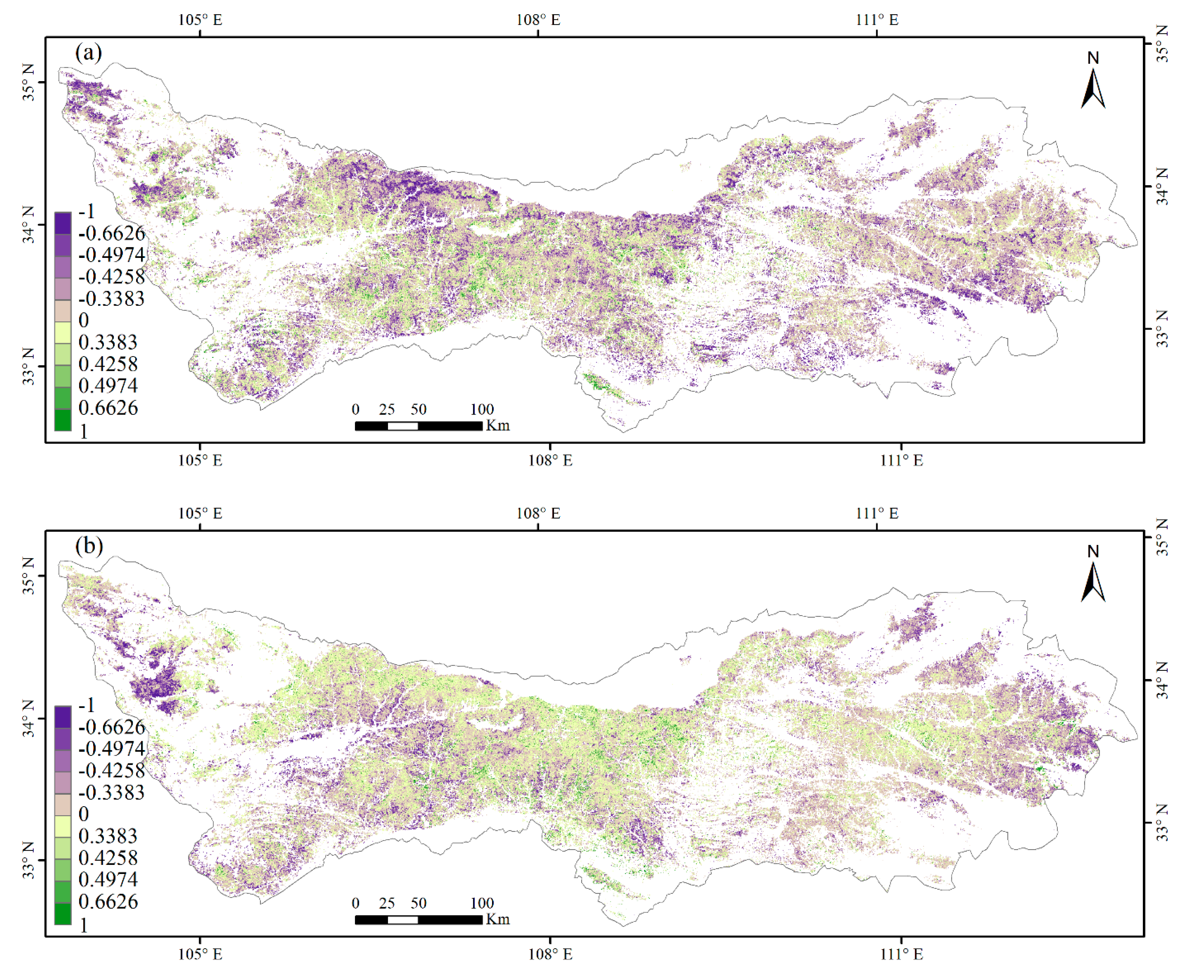
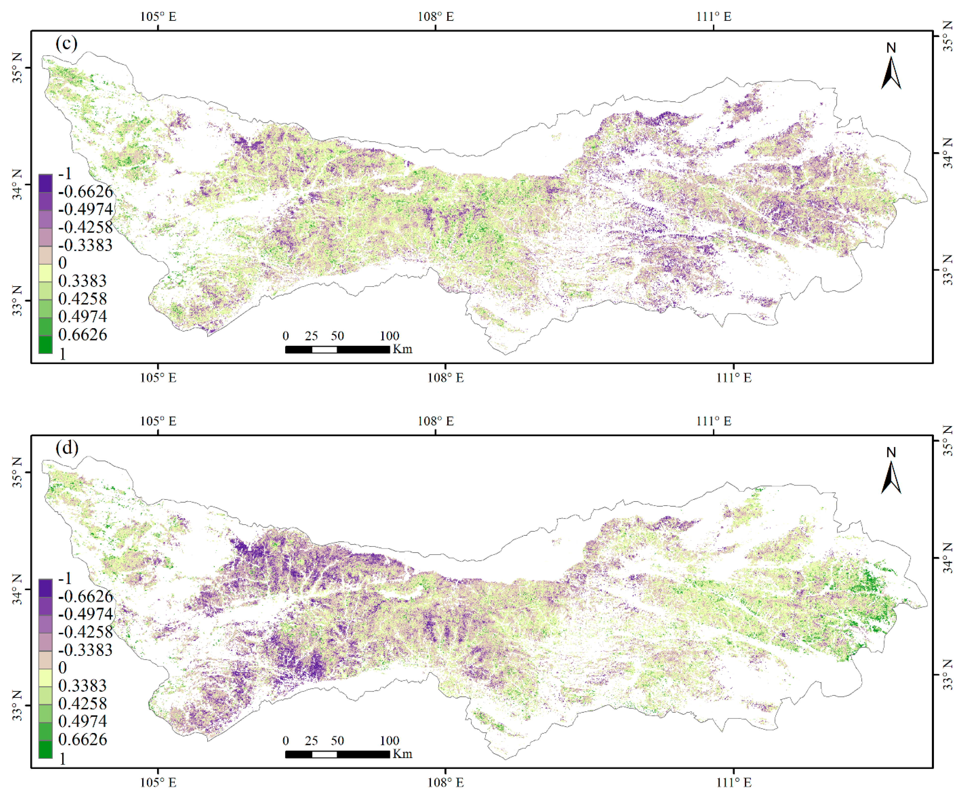
Figure 1. Geographic location and topography of the study area (a), the spatial distribution of the multiyear average temperature (b), and multiyear average precipitation (c).
Forests 10 01007 g001
Figure 2. Spatial patterns of phenology metrics, including the start of the growing season start of growing season (SOS) (a), the end of the growing season end of growing season (EOS) (b), and the length of the growing season length of growing season (LOS) (c), across the Qinling Mountains (QMs) during 2001–2017.
Forests 10 01007 g002aForests 10 01007 g002b
Figure 3. Relationship between elevation and mean SOS (a), EOS (b), and LOS (c) for forests in the QMs from 2001 to 2017. SOS, EOS, and LOS are the abbreviations for the start of the growing season, the end of the growing season, and the length of the growing season, respectively. Warm color represents high point density.
Forests 10 01007 g003
Figure 4. Interannual changes in the mean of the regional-scale SOS (a), EOS (b), and LOS (c). Standard deviation (SD) is indicated by error bars. The red line is the linear fitted line, and the gray section is the confidence level at 95%.
Forests 10 01007 g004
Figure 5. Spatial patterns of the linear trends in SOS (a), EOS (b), and LOS (c) and statistics of the entire linear trends in SOS (d), EOS (e), and LOS (f), from 2001 to 2017 in the QMs. The red, green, and blue lines in (d–f) are the 0, mode and mean values of the trends of SOS, EOS, and LOS, respectively.
Forests 10 01007 g005aForests 10 01007 g005b
Figure 6. Interannual changes in SOS (a), EOS (b), and LOS (c) across altitudinal gradients from 2001 to 2017. Warm color represents high point density.
Forests 10 01007 g006
Figure 7. Spatial patterns of partial correlation coefficients between the SOS (EOS) and preseason mean temperature and accumulated precipitations in the QMs during 2001–2017: (a) partial correlation coefficients between SOS and preseason mean temperatures, controlling for corresponding EOS and accumulated precipitation; (b) partial correlation coefficients between the SOS and preseason accumulated precipitation, controlling for corresponding EOS and mean temperature; (c) partial correlation coefficients between EOS and preseason mean temperatures, controlling for corresponding SOS and accumulated precipitation; (d) partial correlation coefficients between EOS and the preseason accumulated precipitation, controlling for corresponding SOS and mean temperatures. The color-coded values of ±0.6226, ±0.4974, ±0.4258, and ±0.3383 correspond to p-values of 0.01, 0.05, 0.10, and 0.20, respectively, according to two-tailed Student’s t-tests.
Forests 10 01007 g007aForests 10 01007 g007b
Figure 8. Spatial patterns of the sensitivities of the SOS (EOS) to preseason mean temperature and accumulated precipitations in the QMs during 2001–2017: (a) the sensitivities of the SOS to preseason mean temperatures; (b) the sensitivities of the SOS to preseason accumulated precipitation; (c) the sensitivities of the EOS to preseason mean temperatures; (d) the sensitivities of the EOS to accumulated precipitation.
Forests 10 01007 g008aForests 10 01007 g008b
Table 1. Proportions of partial correlation coefficients between the SOS (EOS) and mean temperatures and accumulated precipitations during Lsos, i.e., length of the preseason for SOS (or Leos, i.e., length of the preseason for EOS) for significantly positive correlations (R < 0.4974), not significantly positive correlations (R > 0.4974), not significantly negative correlations (R < −0.4974), and significantly negative correlations (R < −0.4974). Values of R = ± 0.4974 correspond to p-values of 0.05, according to the two-tailed Student’s t-tests.
CorrelationLsosLeos
TemperatureSignificantly Positive Correlation1.6%6.6%
Not Significantly Positive Correlation25.2%49.4%
Not Significantly Negative Correlation60%41.6%
Significantly Negative Correlation13.2%2.4%
PrecipitationSignificantly Positive Correlation1.9%3.2%
Not Significantly Positive Correlation37.6%41.2%
Not Significantly Negative Correlation53.4%48.4%
Significantly Negative Correlation7.1%7.2%

