Article

Potential Effects of Climate Change on Fire Behavior, Economic Susceptibility and Suppression Costs in Mediterranean Ecosystems: Córdoba Province, Spain

by
Juan Ramón Molina
1,*,
Armando González-Cabán
2 and
Francisco Rodríguez y Silva
1
1
Department of Forest Engineering, University of Córdoba, Edificio Leonardo da Vinci-Campus de Rabanales, 14071 Córdoba, Spain
2
Formerly Research Economist at PSW USDA Forest Service, President of Fire Economics and Management Solutions, Riverside, CA 92507, USA
*
Author to whom correspondence should be addressed.
Submission received: 31 May 2019 / Revised: 5 August 2019 / Accepted: 8 August 2019 / Published: 11 August 2019
(This article belongs to the Special Issue Forest Fires under Climate, Social and Economic Changes)

Abstract

:
The potentially large ecological, economic, and societal impacts of climate change makes it a significant problem of the 21st century. These consequences have led to tremendous development in climate change scenarios and new technologies to increase knowledge on the effect and efficiency of mitigation and adaptation measures. Large fires will occur at a higher rate than currently because of lower fuel moisture content resulting in a lower resistance to burning. This is also evidenced by more extreme fire behavior that contributes to higher economic impacts, suppression difficulties and suppression costs. The economic susceptibility concept integrates a set of economic valuation approaches for valuing timber and non-timber resources, considering the fire behavior, and as a consequence, the net value changes for each resource. Flame length increased by 4.6% to 15.69%, according to the different future climate scenarios. Climate change is expected to cause widespread changes to economic susceptibility and suppression costs because of higher flame length and fire intensity. Therefore, our outcomes show an increase in the economic susceptibility of Córdoba Province in the medium and long term (2041–2070) between 6.05% and 25.99%, respectively. In addition, we have found an increase between 65.67% and 86.73% in suppression costs in the last decade. The digital version of the economic susceptibility model using Geographic Information Systems improves its operational capabilities enhancing also its dynamism and simplicity to accept modifications and predictions revisions.

Graphical Abstract

1. Introduction

Nowadays, wildfires have become one of the most significant disturbances worldwide [1,2,3,4,5,6]. The combination of a longer drought period and a higher woody biomass and flammability of dominant species creates an environment conducive to fire spread [7,8]. Furthermore, vegetation pattern changes with the abandonment of traditional rural activities plays a direct role in the increase of fire severity and ecological and economic fire impacts [1,9]. Fire behavior exceeds most frequently firefighting capabilities and fire agencies experience difficulties in suppressing flames while providing safety for both firefighters and citizens [10].
Climate change would have an essential influence on fire regime and ecosystem dynamics [3]. Therefore, long-term projections were carried out using general circulation models (GCMs) [11]. However, projections of extreme events, such as droughts and heatwaves, must be analyzed from studies at regional o local scales [11,12,13]. GCMs involve statistical “downscaling” or an empirical relationship between the general circulation variables and local variables, such as convection process and topography [13,14]. All CGMs results would fluctuate depending on the assumptions of one or another Special Report on Emission scenarios (SREs) based on the economic and technological development and demographic change (A1, A2 and B1 scenarios) [15]. These SREs were superseded by Representative Concentration Pathway scenarios (RCPs) [16]. The four RCPs scenarios, namely RCP2.6, RCP4.5, RCP6 and RCP8.5 were labeled after a possible range of radioactive forcing values in the year 2100 [16].
The last decade in the northern hemisphere has been the hottest since meteorological records began [16]. A temperature increase entails a greater risk of large fires because of the lower fuel moisture content (FMC) and the greater fuel availability [17]. All GCMs show increases in future temperatures, mainly in summer temperatures [18]. Temperature increases to a greater or lesser degree are based on the selected SREs or RCPs. According to the temperature differences, both scenarios can be used to estimate the decrease on FMC. Therefore, a change in fire intensity and severity [1,19], the frequency of large fires [4,20] and the annual area burned [1,19,20,21,22] can be assumed. This expected fire regime change would lead to higher economic impacts [6,23,24,25] and to larger fire suppression difficulties [10,26], and as a consequence, to higher suppression costs [27,28,29]. The increase of suppression difficulties entails the incorporation of a greater number of firefighting resources in order to mitigate fire-line spread. The suppression difficulties index has a strong relation with the energy release from the fire [26]. In this sense, we can affirm that the fire virulence and the suppression difficulty conditions will increase under the different climate change scenarios, and as a consequence, also suppression costs.
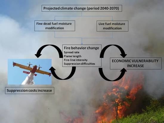
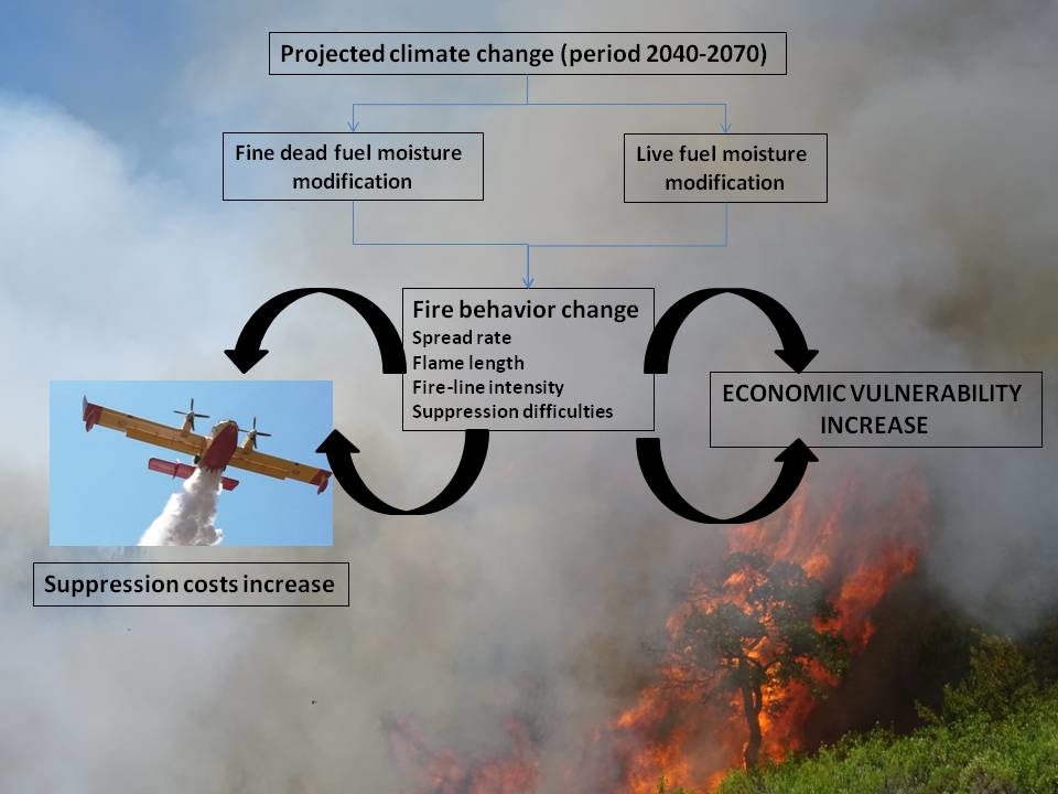
The aim of this study was to identify economic fire susceptibility of tangible assets and suppression costs under projected climate change (period 2041–2070). A general increase in temperatures and decrease in relative humidity was estimated using a downscaling technique. Given the uncertainty of anthropogenic influences, three future scenarios were proposed based on the modified fuel moisture content and fire behavior over the surface and canopy fuels. Fire behavior was modified unevenly under three future scenarios, increasing the economic impacts and suppression costs of forest fires. Therefore, fire susceptibility under the three future scenarios was estimated integrating tangible assets valuation and potential fire behavior, and as a consequence, net value change of the forest resources [30]. Finally, we included a comparative analysis of suppression costs in the study area between different periods. Knowledge of future changes in economic susceptibility and suppression costs is needed for constructing adaptation strategies and for developing efficient fire suppression resources allocation for fire prevention and mitigation activities.

2. Materials and Methods

2.1. Study Area

The study area is Córdoba province, located in southern Spain, with an area of 1,376,150 hectares (Figure 1). The Mediterranean climate is conducive to ignition and propagation of forest fires because of its high summer temperature reaching upwards of 40 °C. This elevated temperature together with a low relative humidity and a very low annual precipitation cause low fuels’ moisture heightening fire ignition risk. In addition to these ignition conditions, wind velocity increases the initial spread of fire, and as consequence, its burned area. For the period of 1990–2018, the fire statistics of Córdoba province show a mean annual number of 114 fires and a mean burned area of 573.22 ha. Over 90% of the Cordoba province’s wildfires are anthropogenic in nature (Forest Department, personal communication). Although our study does not evaluate the increase in fire ignition resulting from the lower fuel humidity, some authors associate the increase in fuel availability with an increase in wildfires [31].
The central part of the province has a gentle topography becoming rugged as we moved southerly or northerly making fire suppression conditions more difficult. Over 80% of the tree cover is dominated by Quercus ilex, in association with Pinus plantations, mainly with P. pinea and P. pinaster. Shrubs are dominated by Cistus spp., in association with Quercus coccifera, Pistacia lentiscus, Phyllirea angustifolia, Arbutus unedo, Olea europaea var. sylvestris, Rosmarinus officinalis, Pistacia terebinthus, Retama shaerocarpa, Teucrium fruticam Thymus mastichina and Lavandula stoechas.

2.2. Climate Scenarios Development

There are different standardized GCMs such as the Third Generation Coupled Global Climate Model (CGCM3) and the European Center model with Hamburg physics (ECHAM5) [16]. For this study, the length of the projections was to extend only to 2070, a time horizon for which the concentration scenario uncertainty is less relevant. We used linear and non-linear methods (statistical downscaling analysis) to establish linear relationships between predictor(s) and predicted [32]. Key inputs include summer data (1961–2000) for both temperature and relative humidity as well as GCM outputs for large-scale variables for future climate. The current period (2001–2018) provides climate information at the study area (weather stations) for which there is appropriate datasets to identify the most interesting GCM output and the best downscaling method. Because of this, we used CGCM3, which produces the most unfavorable temperature for the considered period (2041–2070).
There was a great heterogeneity in the spatial information of the 19 weather stations used, so even very close stations showed significant differences. Then, different statistical downscaling methods can generate different scenarios even when formed with the CGCM3. We evaluated 17 downscaling techniques (Table 1) to extrapolate the weather information to Córdoba province. When using geostatistical extrapolation techniques we used different topographic datasets like altitude, slope and slope-aspect; climate datasets like wind speed and direction; and geographic datasets like forest area (forest and treeless lands), canopy cover (%) and delimitation of watersheds and valleys bottoms. We used 74% of the weather stations to extrapolate temperature and relative humidity (average values in summer period) according to the different downscaling techniques. Finally, we used the remaining 26% of weather stations to test the best predictions based on the mean absolute error.
The absence of future scenarios for fuel moisture and its variability according to each SRE (A1, A2 and B1) and RCP (RCP2.6, RCP4.5, RCP6 and RCP8.5) [36] lead us to identify different scenarios for fuel moisture based on temperature and relative humidity. We proposed three future scenarios for FMC (Table 2) considering different changes in temperature and relative humidity according to each SRE or RCP: an unfavorable scenario (S1), an intermediate scenario (S2) and a favorable scenario (S3). The maximum difference between each SRE and its associated RCP for the study area was 0.4 °C (Table 2) resulting in a fuel moisture decrease between 0.1% and 1%. According to these minor meteorological changes, flame length and suppression costs differences between each SRE and its associated RCP would be minimal.
Using destructive sampling (unpublished dataset and Supplementary Material 1) we identified a wide range of summer records from permanent plots related to fine dead fuel moisture content (FFMC) and live fuel moisture content (LFMC) for the period 2005–2018. Fuel samples were taken during the summer months in Córdoba and oven dried at 70 °C for 72 h [37]. A multiple linear regression was used to develop a model for predicting FFMC from different weather conditions. FFMC was extrapolated to the study area for S1, S2 and S3 based on the most reliable deterministic and geostatistical technique. LFMC depended on the species, the annual weather conditions (temperature, relative humidity and annual precipitation), the slope-aspect and the fuel shading [26]. In a similar way to FFMC, LFMC was directly related to temperature and indirectly related to relative humidity under the same vegetation and similar topographical conditions. Because our objective is not to study in depth the moisture content of live fuels, average LFMC for S1, S2 and S3 was estimated from historical records of the relationship between LFMC, temperature and relative humidity according to the vegetation composition. Dominant species (Supplementary Material 1) in each fuel model or ecosystem and slope and aspect were considered in the estimation of live fuel moisture using a Geographic Information System (GIS).

2.3. Fire Behavior

Fire behavior is a complex phenomenon resulting from the association of meteorological, topographic and vegetation variables [38,39]. Even though socioeconomic changes in land uses and the abandonment of agricultural activities and cattle ranching could cause changes in vegetation combustibility [40], these were not considered. Therefore, vegetation structures (fuel load and species composition) are not significantly influenced by climate change.
In this approach, the impact of FMC decrease on fire behavior is a progressive desiccation of the vegetation and a lower resistance to burn given a heat source. Moreover, the combustion velocity increases (the released water vapor is absorbed faster) as the air is desiccated facilitating fire spread. Therefore, a lower FMC is related to a higher spread rate, flame length and fire intensity. Fire spread simulators such as Farsite©, FlamMap©, Visual Fuego© [39,40] and Visual SEVEIF [41] could be used to estimate the future fire behavior under the three scenarios conditions (S1, S2, S3).

2.4. Economic Susceptibility from Forest Fires

Although the economic valuation should include market and non-market resources [6,23], this study only takes into account tangible assets (both timber and non-timber resources) and carbon storage resource. Tangible assets are measured based on field inventories, historical records or substitute markets. Timber resource impacts were valued using the techniques of the National Fire Management Analysis System (United States Department of Agriculture (USDA) Forest Service) as adapted to the Mediterranean Basin conditions [23] (Table 3). Non-timber losses (acorn or other fruit production and cork production) were valued according to the mean annual production, the estimated resource price and the number of years between the time of the fire and the rotation age or senescence [42] (Table 3). Pasture loss was calculated using the annual income given the site’scarrying capacity, the need of livestock demarcation and the hay price (substitutive market until recovery) [42]. Hunting resource was valued in terms of its sustainable hunting profit, reproductive stock and vegetation resilience [43] (Table 3). Finally, carbon storage losses can be valued like any other tangible assets [25] (Table 3) because they can be traded on the international credit markets (www.sendeco2.com).
This work goes beyond an economic valuation approach because of the integration of the economic valuation of forest resources as well as the net value changes (NVC) [30]. Fire intensity is difficult to measure and validate in field samplings. In this sense, flame length, which is directly related to fire-line intensity [44], can be used as a good indicator of the fire impacts. Flame length is the distance measured from the average flame tip to the middle of the flaming zone at the base of the fire. Visual Fuego [39,40] was used to calculate flame length using weather information from FMC scenarios (S1, S2 and S3) and GIS information to analyze topography and vegetation characteristics. According to flame length and its relationship with fire intensity [44], six intervals or fire intensity levels (FILs) can be represented for easier managerial decision-making. FILs are related to flame length intervals using a percentage depreciation or NVC ratio to estimate the economic susceptibility of each resource [3,20,22,33,34]. Seventeen fires from 1993 to 2015 were used to test the depreciation ratios for each FIL and to identify vegetation resilience (Huétor fire, 1993; Aznalcollar fire, 1995; Los Barrios fire, 1997; Estepona fire, 1999; Cazorla fires, 2001 and 2005; Aldeaquemada fire, 2004; Minas de Rio Tinto fire, 2004; Alajar fire, 2006; Gaucin fire, 2006; Obejo fire, 2007; Orcera fire, 2009; Cerro Vértice, 2011; Coín fire, 2012; Montoro fire, 2013; Alhama fire, 2014; Quesada fire, 2015). GIS allows us to estimate economic susceptibility from fires under the three future FMC scenarios (S1, S2, S3) according to economic valuation of the resources, fire behavior and vegetation resilience.

2.5. Suppression Costs from Forest Fires

The development of a database about suppression resources costs (number of resources and hours in firefighting operations) is difficult, mainly in old wildfires. It is not common in worldwide forest fires statistics to have information about the number of working hours of each suppression resource. For this reason, the studies comparing the costs of suppression over time are a challenging task. However, we have been able to reconstruct the suppression costs of eight large forest fires that occurred in Andalusia region in the last 25 years (between 1993 and 2015). The large fires were as follows: Beas fire: 6176 ha in 1993 (A), Cázulas-Otívar fire: 2258 ha in 1999 (B), Sierra de Lújar fire: 1207 ha in 2000 (C), Mijas fire: 2295.98 ha in 2001 (D), Obejo fire: 4979.15 ha in 2007 (E), Mijas fire 1704.5 ha in 2011 (F), Coín-Marbella fire: 8226 ha in 2012 (G) and Quesada fire: 9760.42 ha in 2015 (H).
For each fire, a dataset was built with type and number of firefighting resources, number of hours worked and official cost by hour of each terrestrial and aerial resource (Supplementary Material 2). Only suppression costs to control the fire were considered, ignoring the travel costs and liquidation costs. Based on the costs dataset, the total suppression cost, the mean cost of terrestrial and aerial resources, the cost per unit area (€/ha) and the cost per unit time were calculated (€/h). We have included a comparative analysis of suppression costs in Andalusia region between 1993 and 2015 in order to identify the climate change effects in relation to suppression costs. SPSS 10© software was used in all analyses. t-test was used to determinate if significant differences (p < 0.05 and p < 0.1) existed in suppression costs between 1990–2005 period (A, B, C and D fires) and last decade (2005–2015 or E, F, G and H fires).

3. Results

3.1. Climate Scenarios Development

Eleven of the 17 downscaling techniques had temperature errors of less than 1 °C for the study area. The Cokigring technique with two datasets (altitude and aspect) had the best results based on the mean absolute error (MAE) and standard deviation from all weather stations used in validation (Figure 2). The 17 downscaling techniques had MAE of less than 4% for relative humidity. In this case, the Cokigring method with two variables (altitude and slope) had the most reliable outcomes (Figure 3).
The CNCM3 estimated an average summer temperature increase between 1.8 and 2.2 °C for the most unfavorable scenario (S1) and an increase between 0.4 °C and 0.8 °C for the most favorable scenario (S3) with respect to the baseline period of 1961–2000. The relative humidity decreased for S1 and S3 scenarios between 6.4% and 9.6% and between 1.8% and 2.8%, respectively. These temperature and relative humidity ranges responded to the size and topographical heterogeneity of the study area.
Our field samplings included a wide range of meteorological conditions according to the most favorable and unfavorable weeks of the period 2005–2018. For precipitation, RCPs change and uncertainty could be found to be large in regions of the world that receive heavy rainfall. In our study area, the summer precipitation (from June to September) is very low (only between zero and three rainy days) (Supplementary Material 3). We have considered zero precipitation in the last 15 days to fuel moisture estimation under actual and projected climate change scenarios. The minimum annual LFMC from summer period ranged from 47.2% to 108.3% for shrubs, and from 65% to 142.6% for trees (Supplementary Material 1). FFMC ranged from 2.78% to 12.1%. We developed two equations to calculate FFMC based on fuel shading: Equation (1) (<50% shading) and Equation (2) (>50% shading) according to 279 summer samples. While Equation (1) had a MAE of 0.89%, Equation (2) showed a MAE of 0.86%.
FFMC = 1.105 + 0.206H − 0.061T   R2 = 0.813
FFMC = 7.919 + 0.119H − 0.101T   R2 = 0.834
where FFMC is the fine dead fuel moisture (%); H is the relative humidity (%) and T is the temperature (°C).
We developed, as discussed earlier, three FMC scenarios (S1, S2, and S3) according to the more or less changes of climate change on FFMC and LFMC (period 2041–2070). These are summarized below.
-
Scenario S1: the change in temperature and relative humidity was the largest (increase of 1.8–2.2 °C and decrease of 6.4%–9.6% with respect to the baseline period of 1961–2000), and as a consequence, the decrease in LFMC was estimated between 8% and 18% according to the dominant species and topographic variables. For FFMC, equations predicted a decrease of 1%–2%.
-
Scenario S2: a drop in the FFMC of 0.7%–1.5% caused by an increase in temperature (1.3%–1.5 °C with respect to the baseline period of 1961–2000) and a decrease in relative humidity (3.3%–5.1%). LFMC could decrease between 5% and 14% according to the dominant species and topographic variables.
-
Scenario S3: equations predicted a decrease of 0.5%–0.8% for the FFMC according to the smallest changes in temperature (0.4%–0.8 °C with respect to the baseline period of 1961–2000) and relative humidity (1.8%–2.8%). LFMC showed a slight decrease from current conditions (0%–5%), but without affecting significantly fire behavior.

3.2. Fire Behavior

According to the comparative analysis of fire behavior simulations between the baseline period (1961–2000) and the three future FMC scenarios (S1, S2 and S3), increases in spread rate and flame length were reported. As an example, Supplementary Material 4 shows the spread rate and flame length differences between the baseline period and S1 scenario for 145 random points. While the average increases in spread rate ranged from 3.35 m/min (S3 scenario) to 12.63 m/min (S1 scenario), the flame length increases varied between 0.22 m (S3 scenario) and 0.94 m (S1 scenario). In regard to these increases in flame length, FIL area was varied by each scenario (Table 4). While the highest area for FIL6 (9.69%) was obtained in S1 scenario, the minimum area for FIL1 (0.45%) was reached under S1 and S2 scenarios. However, the greatest changes were observed in the transition between FIL2 and FIL3 (Table 4). There were significant statistical differences between the baseline period and S1 scenario in relation to spread rate (F = 2.75, p < 0.1), flame length (F = 2.77, p < 0.1) and fire-line intensity (F = 6.6, p < 0.05). Furthermore, there was a significant statistical difference (F = 3.27, p < 0.1) between the baseline period and the intermediate scenario in relation to fire-line intensity.

3.3. Economic Susceptibility from Forest Fires

Although the less severe fires (FIL I and II) could have positive effects on fire-prone ecosystems (e.g., in grassland production resource without the need of livestock exclusion for vegetation regeneration), field samplings showed increases in the NVC according to each FIL (Table 5). At large scale, the increase in flame length and fire intensity led to greater economic impacts. The economic susceptibility of the Córdoba province varied from 981,453,167€ (baseline period) to 1236,541,113€ (S1 scenario) (Table 6). For the study area, the impacts of climate change increased the potential economic impacts between 63,632,966€ (S3 scenario) and 255,087,946€ (S1 scenario) with respect to a baseline period. For the S1 scenario, the most important changes were found in firewood (65,534,622€), carbon storage (48,061,659€) and timber (41,812,106€) (Table 6). For S2 and S3 scenarios, the non-timber resources susceptibility increased between 54,230,349 € and 59,913,688 €. In these cases, the most remarkable changes were measured for the carbon storage (19,227,550–21,088,365€) (Figure 4) and the cork oak (16,944,671–18,090,473€) (Table 6).

3.4. Suppression Costs from Forest Fires

The suppression costs of both terrestrial and aerial resources increased sharply at the beginning of the 21st century. Because of this, the cost per unit area and the cost per unit time between Fire A and Fire H showed an increase of 86.73% and of 65.67%, respectively (Table 7). Significant statistical differences were found between fires that occurred between 1995–2005 and fires that occurred in the last decade (Table 8) in relation to the number of hours worked to control the fire (t = −0.99, p < 0.05), aerial resources costs (t = −1.86, p < 0.05), total suppression costs (t = −1.68, p < 0.1) and suppression cost per unit time ( t= −1.88, p < 0.1).

4. Discussion

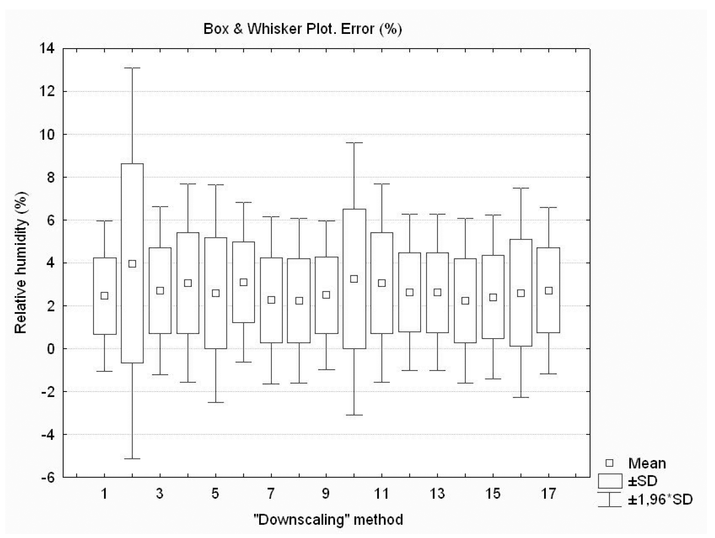
The climate scenarios generated for the first seven decades of the century present robust estimates for temperature [13,16]. RCP 2.6 changes are much lower than the rest of the RCPs because it includes the option of using policies to achieve net negative carbon dioxide emissions before the end of the century [16,36]. Geostatistical methods using GIS play an important role for extrapolating the climate scenarios to any territory [33,34,35]. Results for our study area shows an increase in the summer temperatures similar to those obtained in other Mediterranean studies [8,16,18,46]. In recent summers, field inventories in Mediterranean basin have shown values generally smaller than standard values observed for FFMC and LFMC [47,48]. According to our results, FFMC and LFMC could decrease between 0% and 2% and between 8% and 18%, respectively. The decrease in FMC has an important effect on fire behavior, and as a consequence, in the large fires’ occurrence [1,3,4,19,20,21,22]. The integrated use of GIS and fire spread simulators allows us to analyze fire behavior under different FMC scenarios [39,40,41]. Our FMC scenarios showed more severe fire behavior in a similar way than other studies [1,19,20]. Flame length increased from 4.60% to 15.69%, and as a consequence, fire-line intensity increased considerably, ranging from 9.81% to 21.31%. Finally, climate change would raise spread rate between 4.45% and 24.07%. Some studies have shown the effects of climate change in fire intensity and difficulties in suppression flames [10] and, therefore, in an increase in the economic impacts from wildfires [6,9,24,25].
The goal of this manuscript has not been to make a dissertation on the consequences of climate change on the socioeconomics of potentially affected Mediterranean ecosystems. However, we consider that the effects of climate change in increasing the intensity and severity of forest fires, imply a greater demand for budgets to increase the contracting of resources from suppression activities. It also implies an increase in the duration of contracts over the months. The effects are of a reduction in the same proportion of the budget allocated to fire prevention and management activities in the fuel treatment. The administrations and departments of prevention and extinction of forest fires have difficulties to obtain increases of budgets to extinction and fire suppression without affecting in reductions in the budgets of prevention. This circumstance is today a reality verified throughout the last 50 years. In addition, and as already demonstrated in the manuscript, the increase in the difficulty of suppression actions is generating a progressive increase in suppression costs.
Unquestionably, the increase in the intensity and severity of forest fires due to climate change [1,9,40] and the high availability of forest fuels (abandonment of the rural environment and decrease in population density) would increase natural resources impacts. In this sense, disturbances and negative effects affect the income of populations when resources such as leisure and recreation are damaged by the strong alteration of the landscape after the fires, in the same way erosion and loss of water quality, are damages in forest landscapes that indirectly imply negative effects on the socioeconomics of the populations affected. On the other hand, one might think that forest restoration work on landscapes affected by fires can be a positive consequence from a socioeconomic point of view, increasing the wages and jobs in the rural economy. This is not entirely true for two reasons: first, the strong budgetary decapitalization of governments and administrations makes it difficult to approve budgets in order to address the financing of restoration work on the large areas affected by large forest fires. Consequently, the generation of job opportunities is not clear. Secondly and from the point of view of investigations of the causes of the forest fires over more than 50 years, important efforts have been made to avoid relating forest fires to the socio-economic benefit of increasing wages for extinction, prevention and the restoration. These control actions are aimed at reducing the arson fires causes. From our point of view, it is difficult to find positive socio-economic effects of climate change on forest fires. Perhaps it could be indicated as a positive effect, the change in the combustibility that occurs in the landscapes affected by large fires, decreasing of high intensity fires in the following decades, so the slow recovery of damaged resources. It will be guaranteed in one way or another, as well as the protection and defense of populations located in forest areas.
The economic susceptibility of the forest resources in the study area is about 918 million Euros according to the baseline period. Fire impacts pointed to the importance role that carbon storage (22.10% of the total loss), timber (21.34%) and firewood (20.67%) resources play in the rural study area. The effect of climate change on individual resources is uneven. For example, while acorn production impact increases considerably (Table 6), chestnut production impact is slightly affected, due in part to its location in humid areas filled with debris and isolated understory. Some resources, such as cork oak, pasture production and game, have shown few changes under the favorable and intermediate scenarios (S2 and S3 scenarios), but larger changes for the most unfavorable scenario (S1 scenario). As an example, a livestock exclusion is needed in pasture production resource for the highest fire intensity levels [41,44]. It can be observed in the differences between baseline period, S2 and S3 scenarios and S1 scenario (an increase of 46% of the economic impacts). In general, climate change would increase the economic susceptibility of the study area between 63,632,966€ or 6.05% (baseline period-S3 scenario) and 255,087,946 or 25.99%€ (baseline period-S1 scenario) (Table 9).
Climate change has accentuated the virulence and the suppression of difficulties of large fires leading to an increase of suppression costs [27,28,29,49]. Although there is a wide burned area range according to the standard deviation, an upward trend can be seen in the last decade in relation to burned area (6167 ha compared with 2984 ha) and burned area per unit time (88.56 ha/h compared with 59.60 ha/h) (Table 6). These burned area trends and the significant statistical difference found in the control time (95.75 h compared with 49.25 h) seem to suggest that there is an increase in suppression difficulties [26]. Significant statistical differences were found between 1990–2005 large fires and 2005–2015 large fires from total suppression costs and suppression costs per unit time. The comparative analysis confirmed a general increase in cost per unit area (86.73%) and cost per unit time (65.67%), mainly in relation to the increase in aerial resources cost (818,348€ compared to 110,706.01€). This increase in aerial firefighting operations responds both to the number of aircraft and to the number of hours worked between the two time periods considered. According to fire size costs, we found an average rate of 1.41-fold increased suppression costs between the two time periods considered. It is an interesting outcome that suppression costs have increased in recent years in association with a decrease on FMC was induced by an increase in temperature and a decrease in relative humidity.
Suppression costs are based on the real data and official prices for the study area. In this sense, our findings highlight the increase of suppression costs in the last decade. The average suppression cost per fire size [49] can offer the possibility to study in depth the behavior of the suppression costs over time based on fire size. Measuring techniques would have most likely greatly improved for the time period considered (2041–2070). Although fire suppression techniques have improved from 1990 to 2019, fire suppression costs have increased as reported in this and other studies [27,28,29,49]. However, increase fire suppression efficiency has not been demonstrated in part due to the generalized decision to send more and more fire suppression resources to fires without knowledge of the resources’ efficiency [50,51]. This practice is more evident in high-intensity large wildfires increasing fire suppression costs without a corresponding increase in suppression activities efficiency.
At present, fire suppression costs for the study area in general represent about 65% of the total fire management budget [52]. The increase in fire intensity leads to higher economic impacts and suppression difficulties [6,10,24,25], which if not considered leads to higher suppression costs [1]. Our research only considered suppression costs’ changes. Further studies should include the prevention costs and the relationship between prevention and suppression efforts and costs. Because the important short- and long-term effects and the higher risk of large fires, the national and regional agencies and/or authorities have requested estimations on fire susceptibility and suppression difficulties of wildfires in relation to climate change. Our approach identifies sectors and resources with the highest future economic susceptibility for the considered period (2041–2070). This strategic information plays an essential role in operational priorities and firefighting resources management to increase the efficiency in the provision of fire services and to mitigate the fire impacts. The use of GIS tools increases the flexibility of this approach to include new forest resources and net value changes enabling a further extrapolation to any study area.

5. Conclusions

Climate change plays a key role in the medium- and long-term forest fire management. There is a future upward trend in the number and frequency of large fires that looms even larger because of the higher spread rate, flame length and fire-line intensity according to the climate change scenarios used here. The potentially resulting fire regime leads to significantly increased economic fire impacts, fire suppression difficulties, and fire suppression costs, mainly in relation to aerial firefighting resources. Climate change should be considered in fire-management policies for mitigation and adaptation of potential economic susceptibility by prioritization of fuel treatments. The economic susceptibility of the territory in the medium term (2041–2070) allows us to optimize preventive activities and to find an efficient spatial-temporal allocation of suppression resources. The availability of GIS eases the possibility to make changes and adaptations given new or updated climate scenarios and different management needs, making it a valuable tool in fire management and prevention programs.

Supplementary Materials

The following are available online at https://0-www-mdpi-com.brum.beds.ac.uk/1999-4907/10/8/679/s1: Electronic Supplementary Material 1: live fuel moisture for fire behavior simulation, Electronic Supplementary Material 2: inputs data for assessing suppression costs, Electronic Supplementary Material 3: potential effects on spread rate and flame length, Electronic Supplementary Material 4: Potential effects on flame length.

Author Contributions

J.R.M. contributed to the methodology, formal analysis, data curation and original draft preparation. A.G.-C. participated in conceptualization, methodology and writing—review and editing. F.R.S. contributed to the methodology, formal analysis, supervision and funding acquisition.

Funding

This research was funded by the National Institute for Agricultural Research (INIA) from the Spanish Ministry of Science and Innovation and cofounded by FEDER funds (VIS4FIREproject (RTA2017-00042-C05-01).

Acknowledgments

We thank two anonymous reviewers and the Assistant Editor for their help in improving presentation of this paper.

Conflicts of Interest

The authors declare no conflict of interest.

References

  1. Flannigan, M.D.; Krawchuk, M.A.; De Groot, W.J.; Wotton, B.M.; Gowman, L.M. Implications of changing climate for global wildland fire. Int. J. Wildland Fire 2009, 18, 483–507. [Google Scholar] [CrossRef]
  2. Pechony, O.; Shindell, T. Driving forces of global wildfires over the past millennium and the forthcoming century. Proc. Natl. Acad. Sci. USA 2010, 45, 19167–19170. [Google Scholar] [CrossRef] [PubMed]
  3. Pausas, J.G.; Fernández-Muñoz, S. Fire regime changes in the Western Mediterranean Basin: From fuel-limited to drought-driven fire regime. Clim. Chang. 2012, 110, 215–226. [Google Scholar] [CrossRef]
  4. Cardil, A.; Molina, D.; Kobziar, L.N. Extreme temperature days and their potential impacts on southern Europe. Nat. Hazards Earth Syst. 2014, 14, 3005–3014. [Google Scholar] [CrossRef] [Green Version]
  5. Boer, M.; Nolan, R.; Resco, V.; Clarke, H.; Price, O.; Bradstock, R. Changing weather extremes call for early warning of potential for catastrophic fire. Earth Future 2017, 5, 1196–1202. [Google Scholar] [CrossRef]
  6. Molina, J.R.; Moreno, R.; Castillo, M.; Rodríguez y Silva, F. Economic susceptibility of fire-prone landscapes in natural protected areas of the southern Andean range. Sci. Total Environ. 2018, 619, 1557–1565. [Google Scholar] [CrossRef] [PubMed]
  7. Piñol, J.; Terradas, J.; Lloret, F. Climate warming, wildfire hazard and wildfire occurrence in coastal eastern Spain. Clim. Chang. 1998, 38, 345–357. [Google Scholar] [CrossRef]
  8. Millán, M.M.; Estrela, M.J.; Sanz, M.J.; Mantilla, E. Climatic feedbacks and desertification: The Mediterranean model. J. Clim. 2005, 18, 684–701. [Google Scholar]
  9. Chuvieco, E.; Martínez, S.; Román, M.V.; Hantson, S.; Pettinari, M.L. Integration of ecological and socio-economic factors to assess global vulnerability to wildfire. Glob. Ecol. Biogeogr. 2014, 23, 245–258. [Google Scholar] [CrossRef]
  10. Werth, P.A.; Potter, B.E.; Alexander, M.E.; Cruz, M.; Clements, C.B.; Finney, M.; Forthofer, J.M.; Scott, L.G.; Hoffman, C.; Jolly, W.M.; et al. Synthesis of Knowledge of Extreme Fire Behavior: Volume 2 for Fire Behavior Specialists, Researchers, and Meteorologists; General Technical Report PNW-GTR-891; Pacific Northwest Research Station, USDA Forest Service: Corvallis, OR, USA, 2016; p. 258.
  11. Huebener, H.; Cubasch, U.; Langematz, U.; Spangehi, T.; Nierhorstr, F.; Fast, I.; Kunze, M. Ensemble climate simulations using a fully coupled ocean–troposphere–stratosphere general circulation model. Philos. Trans. R. Soc. A 2007, 365, 2089–2101. [Google Scholar] [CrossRef]
  12. Trigo, R.; Palutikof, J. Precipitation scenarios over Iberia: A comparison between direct GCM output and different downscaling techniques. J. Clim. 2001, 14, 4422–4446. [Google Scholar] [CrossRef]
  13. Ribalaygua, J.; Torres, L.; Del Carre, M. La generación de escenarios locales de clima futuro orientados a la definición de estrategias de adaptación al cambio climático en el ámbito forestal. Rev. Montes 2008, 92, 11–18. [Google Scholar]
  14. Hertig, E.; Jacobeit, J. Assessments of Mediterranean precipitation changes for the 21st century using statistical downscaling techniques. Int. J. Climatol. 2007, 8, 1025–1045. [Google Scholar] [CrossRef]
  15. Nakicenovi, N.; Swart, R. Special Report on Emissions Scenarios; Intergovernmental Panel on Climate Change, Cambridge University Press: Cambridge, UK, 2000; p. 599. [Google Scholar]
  16. IPCC. Climate Change 2014: Synthesis Report. Contribution of Working Groups I, II and III to the Fifth Assessment Report of the Intergovernmental Panel on Climate Change; Core Writing Team, Pachauri, R.K., Meyer, L.A., Eds.; IPCC: Geneva, Switzerland, 2014; p. 151. [Google Scholar]
  17. Jurdao, S.; Chuvieco, E.; Arevalillo, J.M. Modelling Fire Ignition Probability from Satellite Estimates of Live Fuel Moisture Content. Fire Ecol. 2012, 8, 77–97. [Google Scholar] [CrossRef]
  18. Van der Linden, P.; Mitchell, J.F.B. (Eds.) ENSEMBLES: Climate Change and Its Impacts: Summary of Research and Results from the ENSEMBLES Project; Met Office Hadley Centre: Exeter, UK, 2009; p. 160.
  19. Flannigan, M.D.; Amiro, B.D.; Logan, K.A.; Stocks, B.J.; Wotton, B.M. Forest fires and climate change in the 21st century. Mitig. Adapt. Strateg. Glob. Change 2006, 11, 847–859. [Google Scholar] [CrossRef]
  20. Westerling, L.; Hidalgo, H.G.; Cayan, D.R.; Swetnam, T.W. Warming and earlier spring increase western U.S. forest wildfire activity. Science 2006, 18, 940–943. [Google Scholar] [CrossRef]
  21. Running, S.W. Is global warming causing more, larger wildfires? Science 2006, 18, 927–928. [Google Scholar] [CrossRef]
  22. Moreno, V.; Conedera, M.; Chuvieco, E.; Pezzatti, G. Fire regime changes and major driving forces in Spain from 1968 to 2010. Environ. Sci. Policy 2014, 37, 11–22. [Google Scholar] [CrossRef]
  23. Rodríguez-Silva, F.; Molina, J.R.; González-Cabán, A.; Herrera, M.A. Economic vulnerability of timber resources to forest fires. J. Environ. Manag. 2012, 100, 16–21. [Google Scholar] [CrossRef]
  24. Castillo, M.; Molina, J.R.; Rodríguez y Silva, F.; García-Chevesich, P.; Garfias, R. A system to evaluate fire impacts from simulated fire behavior in Mediterranean areas of Central Chile. Sci. Total Environ. 2017, 579, 1410–1418. [Google Scholar] [CrossRef]
  25. Molina, J.R.; Herrera, M.A.; Rodríguez y Silva, F. Wildfire-induced reduction in the carbon storage of Mediterranean ecosystems: An application to brush and forest fires impacts assessment. Environ. Impact Assess. 2019, 76, 88–97. [Google Scholar] [CrossRef]
  26. Rodríguez y Silva, F.; Molina, J.R.; González-Cabán, A. A methodology for determining operational priorities for prevention and suppression of wildland fires. Int. J. Wildland Fire 2014, 23, 544–554. [Google Scholar] [CrossRef]
  27. Association for Fire Ecology. Reduce Wildfire Risks or We’ll Continue to Pay More for Fire Disasters; International Association of Wildland Fire, The Nature Conservancy: Missoula, MT, USA, 2015; p. 13. Available online: http://fireecology.org/Resources/Documents/Reduce-WIldfire-Risk-16-April-2015-Final-Print.pdf (accessed on 23 May 2019).
  28. Ellison, A.; Moseley, C.; Bixler, R.P. Drivers of Wildfire Suppression Costs. Literature Review and Annotated Bibliography; Ecosystem Workforce Program Working: Eugene, OR, USA, 2015; p. 36. [Google Scholar]
  29. Forest Service. The Rising Cost of Wildfire Operations. Effects on the Forest´s Service Non-Fire Work. Fire Budget Report; United States Department of Agriculture: Washington, DC, USA, 2015; p. 16. Available online: https://www.fs.fed.us/sites/default/files/2015-Fire-Budget-Report.pdf (accessed on 23 May 2019).
  30. Rodríguez y Silva, F.; González-Cabán, A. SINAMI: A tool for the economic evaluation of forest fire management programs in Mediterranean ecosystems. Int. J. Wildland Fire 2010, 19, 927–936. [Google Scholar] [CrossRef]
  31. Wotton, B.M.; Martell, D.L.; Logan, K.A. Climate change and people-caused forest fire occurrence in Ontario. Clim. ChangE 2013, 60, 275–295. [Google Scholar] [CrossRef]
  32. Trzaska, S.; Schnarr, E. A Review of Downscaling Methods for Climate Change Projections; Tetra Tech ARD, Center for International Earth Science Information Network (CIESIN): Burlington, VT, USA, 2014; p. 42. [Google Scholar]
  33. Molina, J.R. Integración de Herramientas para la Modelización Preventiva y Socioeconomica del Paisaje Forestal Frente a los Incendios Forestales en Relación con el Cambio Climático. Ph.D. Thesis, University of Córdoba, Cordoba, Spain, 2008. [Google Scholar]
  34. Bakış, R.; Bayazıt, Y.; Uyguçgil, H.; Koç, C. Mapping of Precipitation, Temperature and Evaporation Distributions in the Porsuk Basin Using Distant Forecasting Methods. Comput. Water Energy Environ. Eng. 2017, 6, 321–350. [Google Scholar] [CrossRef] [Green Version]
  35. Jo, A.; Ryu, J.; Chung, H.; Choi, Y.; Jeon, S. Applicability of various interpolation approaches for high resolution spatial mapping of climate data in Korea. Int. Arch. Photogramm. Remote Sens. Spat. Inf. Sci. 2018, 12, 703–710. [Google Scholar] [CrossRef]
  36. Rogelj, J.; Meinshausen, M.; Knutti1, R. Global warming under old and new scenarios using IPCC climate sensitivity range estimates. Nat. Clim. Chang. 2012, 2, 248–253. [Google Scholar] [CrossRef]
  37. Elvira, L.M.; Hernando, C. Inflamabilidad y Energía de las especies del Sotobosque (Estudio Piloto con Aplicaci6n a los Incendios Forestales); Monografías INIA 68; Ministerio De Agricultura, Pesca y Alimentación: Madrid, Spain, 1989; p. 99. [Google Scholar]
  38. Rothermel, R.C. A Mathematical Model for Predicting Fire Spread in Wildland Fuels; Research Paper INT-115; USDA Department of Agriculture, Intermountain Forest and Range Experiment Station: Ogden, UT, USA, 1972; p. 40.
  39. Finney, M. FARSITE: Fire Area Simulator—Model Development and Evaluation; Research Paper RMRS-RP-4 Revised; USDA Forest Service, Rocky Mountain Research Station: Missoula, MT, USA, 2004; p. 47.
  40. Rodríguez y Silva, F.; Molina, J.R. Modeling Mediterranean forest fuels by integrating field data and mapping tools. Eur. J. For. Res. 2012, 131, 571–582. [Google Scholar] [CrossRef]
  41. Rodríguez y Silva, F.; Molina, J.R.; Rodríguez, J. The efficiency analysis of the fire control operations using Visual SEVEIF tool. In Advances in Forest Fire Research; Viegas, D.X., Ed.; University of Coimbra: Coimbra, Portugal, 2014; pp. 1883–1894. [Google Scholar]
  42. Molina, J.R.; Herrera, M.A.; Zamora, R.; Rodríguez y Silva, F. González-Cabán, A. Economic losses to Iberian swine production from forest fires. For. Policy Econ. 2011, 13, 614–621. [Google Scholar] [CrossRef]
  43. Zamora, R.; Molina-Martínez, J.R.; Herrera, M.A.; Rodríguez y Silva, F. A model for wildfire prevention planning in game resources. Ecol. Model. 2010, 221, 19–26. [Google Scholar] [CrossRef]
  44. Alexander, M.; Cruz, M. Interdependencies between flame length and fireline intensity in predicting crown fire initiation and crown scorch height. Int. J. Wildland Fire 2012, 21, 95–113. [Google Scholar] [CrossRef]
  45. Molina, J.R.; Rodríguez y Silva, F.; Herrera, M.A. A simulation tool for socio-economic planning on forest fire suppression management. In Forest Fires Detection, Suppression and Prevention; Gómez, E., Álvarez, K., Eds.; Nova Science Publishers: New York, NY, USA, 2009; pp. 33–88. [Google Scholar]
  46. Miró, J.J.; Estrela, M.J.; Millán, M. Summer temperature trends in a Mediterranean area (Valencia region). Int. J. Climatol. 2006, 26, 1051–1073. [Google Scholar] [CrossRef]
  47. Castro, F.X.; Tudela, A.; Sebastià, M.T. Modeling moisture content in shrubs to predict fire risk in Catalonia (Spain). Agr. For. Meteorol. 2003, 116, 49–59. [Google Scholar] [CrossRef]
  48. Bilgili, E.; Alperen, K.; Usta, Y.; Göltas, M. Diurnal surface fuel moisture prediction model for Calabrian pine stands in Turkey. IForest 2019, 12, 262–271. [Google Scholar] [CrossRef]
  49. Florec, V.; Thompson, M.P.; Rodríguez y Silva, F. Cost of Suppression. In Encyclopedia of Wildfires and Wildland-Urban Interface (WUI) Fires; Manzello, S., Ed.; Springer: Cham, Switzerland, 2019; Available online: https://0-doi-org.brum.beds.ac.uk/10.1007/978-3-319-51727-8_96-1 (accessed on 29 May 2019).
  50. Plucinski, M. Fighting flames and forging firelines: Wildfire suppression effectiveness at the fire edge. Curr. For. Rep. 2019, 5, 1–19. [Google Scholar] [CrossRef]
  51. Plucinski, M. Contain and control: Wildfire suppression effectiveness at incidents and cross landscapes. Curr. For. Rep. 2019, 5, 20–40. [Google Scholar] [CrossRef]
  52. Greenpeace. Protege el Bosque, Protegetu Casa; InformeAmpliado Greenpeace: Amsterdam, The Netherlands, 2017; p. 140. Available online: https://es.greenpeace.org/es/sala-de-prensa/informes/protege-el-bosque-protege-tu-casa/ (accessed on 1 July 2019).
Figure 1. Study area location with selected weather stations.
Forests 10 00679 g001
Figure 2. Estimated mean absolute errors (MAE) for temperature using different deterministic and geostatistical methods. The 11 methods used were: (1) Inverse Distance Weighting; (2) Global Polynomial Interpolation; (3) Local Polynomial Interpolation; (4) Kriging; (5) Cokriging (altitude); (6) Cokriging (altitude, forest area); (7) Cokriging (altitude, aspect); (8) Cokriging (altitude, slope, forest area); (9) Cokriging (altitude, slope); (10) Cokriging (slope, aspect); (11) Cokriging (altitude, slope, aspect).
Forests 10 00679 g002
Figure 3. Estimated mean absolute errors (MAE) for relative humidity using different deterministic and geostatistical methods. The 17 methods used were: (1) Global Polynomial Interpolation; (2) Inverse Distance Weighting; (3) Local Polynomial Interpolation; (4) Kriging; (5) Cokriging (altitude, aspect); (6) Cokriging (altitude); (7) Cokriging (altitude, slope, wind speed); (8) Cokriging (altitude, slope); (9) Cokriging (altitude, slope, aspect); (10) Radial Basis Functions; (11) Cokriging (altitude, slope, canopy cover); (12) Cokriging (altitude, slope, forest area); (13) Cokriging (altitude, aspect, forest area); (14) Cokriging (altitude, slope, wind direction); (15) Cokriging (altitude, slope, valley bottom); (16) Cokriging (slope, aspect); (17) Cokriging (altitude, slope, watersheds).
Forests 10 00679 g003
Figure 4. Economic susceptibility of carbon storage under baseline period and S1 scenario for Córdoba province.
Forests 10 00679 g004
Table 1. Statistical downscaling techniques applied for the study area.
Downscaling TechniqueVariablesReference
Global Polynomial InterpolationTemperature, relative humidity[33]
Inverse Distance WeightingTemperature, relative humidity[33,34,35]
Local Polynomial InterpolationTemperature, relative humidity[33]
Radial Basis FunctionsTemperature, relative humidity[33]
KrigingTemperature, relative humidity[33,34,35]
CokrigingTemperature, relative humidity, altitude[33,34,35]
CokrigingTemperature, relative humidity, altitude, aspect[33,34,35]
CokrigingTemperature, relative humidity, altitude, slope[33,34,35]
CokrigingTemperature, relative humidity, slope, aspect[33,34,35]
CokrigingTemperature, relative humidity, altitude, slope, aspect[33,34,35]
CokrigingTemperature, relative humidity, altitude, slope, wind speed[33,34,35]
CokrigingTemperature, relative humidity, altitude, slope, canopy cover[33,34,35]
CokrigingTemperature, relative humidity, altitude, slope, forest area[33,34,35]
CokrigingTemperature, relative humidity, altitude, aspect, forest area[33,34,35]
CokrigingTemperature, relative humidity, altitude, slope, wind speed[33,34,35]
CokrigingTemperature, relative humidity, altitude, slope, valley bottom[33,34,35]
CokrigingTemperature, relative humidity, altitude, slope, watersheds[33,34,35]
Table 2. New fuel moisture content (FMC) scenarios created based on Special Report on Emission (SRE) and Representative Concentration Pathway (RCP) scenarios.
FMC ScenarioSRE ScenarioTemperature Increase (°C)Relative Humidity Decrease (%)RCP ScenarioTemperature Increase (°C)Relative Humidity Decrease (%)
S1A11.8–2.26.4–9.6RCP 8.51.8–2.66.4–11.3
S2B21.3–1.53.3–5.5RCP 6.00.8–1.82.1–6.1
S3B10.4–0.81.8–2.8RCP 2.60.5–1.22.2–4.2
Table 3. Formulations used for economic valuation.
ResourceFormulaPotential StatusSource
TimberL = (a*S*N)/(S + b*N)Immature and mature stands[23]
S = C0*t [re + i(re − 1)] + F*(re − 1)Immature stands
N = [(P*V*1.025y)/1.04y] * [1 − (1.025/1.04)e] * [1 + M*c*t]Immature stands
S = [P*V − P1*V1] + P*V [(r(R-e) − 1)/(r(R−e))]Mature stands
N = V*c*t [C*P + (1 − C)*P1]Mature stands
Firewood; fruit productionL = Ap*Pr* [((1 + r)y − 1)/(r*(1 + r)y]Mature stands[42]
Pasture productionL = V* [((1 + 0.06)n − 1)/(0.06*(1 + 0.06)n]Livestock area[42]
Hunting activityL = V* [((1 + 0.06)n − 1)/(0.06*(1 + 0.06)n] + StGame area[43]
Carbon storageL = 3.67*CS*Pc + AS [((1 + r)(R-e) − 1)/(r*(1 + r) (R−e)]Woodlands[25]
where “L” is the resource loss (€/ha), “S” is the valuation according the Spanish system (€/ha), “N” is the valuation adapted from NFMAS (National Fire Management Analysis System, €/ha), “a” takes the value of 1.7 or 2.6 according to protection or recreational function, or timber forest respectively, “b” takes the value of 0.85 or 0.25 base on the same reasons, “C0” is the reforestation cost per hectare (€/ha), “t” is the percentage burned stand based on fire behavior, “r” is the compound annual interest rate and depends on species growth rate: fast growth (1.06), medium growth (1.04), slow growth (1.025) and very slow growth (1.015) [20]; “e” is the estimated stand age, “i” is the annual silvicultural cost factor and depends on species growth rate: fast growth (1.27), medium growth (1.1) slow growth (1.1) and very slow growth (0.93), “P” is the price of the timber (€/m3), “V” is the timber volume (m3/ha), “y” is the time or years remaining in the harvesting rotation or senescence age, “M” is the tree mortality coefficient depending on fire intensity, “c” is the percentage of immature or mature timber in stand, “P1” is the price of affected timber with commercial use (€/m3), “V1” is the volume of burned timber (m3/ha), “R” is the rotation age, “C” is the percent of non-commercial timber, “Ap” is the annual production (kg/ha), “Pr” is the estimated resource price (€/kg), “V” is the annual income given the carrying capacity of the site (€/ha), “n” is the estimated number of years until recovery (vegetation resilience), “St” is the reproductive stock (€/ha), “CS” is the carbon stock when the fire occurs, “Pc” is the carbon price and “AS” is the annual growth rate on carbon storage.
Table 4. Fire intensity level (FIL) area (%) estimated to the baseline period and the FMC scenarios.
Flame Length (m)FILBaseline (%)S1 (%)S2 (%)S3 (%)
<2I0.470.450.450.47
2–3II44.439.6243.4443.44
3–6III27.0859.9325.7727.39
6–9IV14.193.908.767.58
9–12V11.1516.4014.0313.56
>12 mVI2.699.697.567.56
Table 5. Net value change (NVC) (%) of each resource based on fire intensity level (FIL).
ResourceFIL IFIL IIFIL IIIFIL IVFIL VFIL VI
Timber 18.33 (±6.58)16.65 (±5.89)38.58 (±6.27)57.85 (±13.74)82.79 (±1.81)89.41 (±2.82)
Firewood 24.5 (±0.71)9 (±1.41)18.2 (±4.25)52.5 (±10.61)66.1 (±6.42)77.5 (±6.53)
Fruit production 35.83 (±1.44)11.67 (±2.88)24.67 (±9.23)48.75 (±1.76)68.16 (±1.60)80.17 (±1.25)
Cork oak 47.5 (±3.53)15 (±7.07)30 (±21.21)47.5 (±24.74)67.5 (±14.73)80 (±14.14)
Pasture 5--85100100100
Game 62045658595100
Carbon storage 758.02 (±11.89)58.02 (±11.89)70.38 (±12.05)83.7 (±4.28)98.75 (±2.62)98.75 (±2.62)
1 NVC obtained from [23] 2 NVC obtained from [33] and the following new experiences: Orcera fire (2009), Cerro Vértice fire (2011), Coín fire (2012), Montoro fire (2013), Alhama fire (2014) and Quesada fire (2015) 3 NVC obtained from [42] and the following new experiences: Cerro Vértice fire (2011), Coín fire (2012), Montoro fire (2013), Alhama fire (2014) and Quesada fire (2015) 4 NVC obtained from [45] 5 NVC obtained from [42] and the following new experiences: Montoro fire (2013) and Quesada fire (2015) 6 NVC obtained from [43] 7 NVC obtained from [25].
Table 6. Economic susceptibility of Córdoba province according to the baseline period and S1, S2 and S3 scenarios.
ResourcesScenarios
Baseline Period (€)S1 (€)S2 (€)S3 (€)
Timber resources209,465,938251,278,044220,149,121218,868,555
Firewood202,849,328286,383,950219,508,148217,581,960
Pine nut12,672,78514,550,16413,525,40913,459,315
Acorn fruit75,337,855111,376,16077,695,22277,166,375
Chestnut36,84237,24937,24936,842
Cork oak182,061,413215,807,738200,151,886199,006,084
Pasture (grazing activity)49,368,73472,126,91549,455,44949,445,321
Game (hunting activity)32,761,16238,020,12433,539,80933,395,021
Carbon storage216,899,110264,960,769237,987,745236,126,660
Table 7. Suppression costs for each large fire studied.
Forest Fire ABCDEFGH
Burned area (ha)6176.002258.001207.002295.981704.508226.004979.159760.42
Control time * (h) 57.0053.0051.0036.0036.0042.0072.00233.00
Burned area/hour (ha/h)108.3542.6023.6763.7847.35195.8669.1541.89
Terrestrial resources (€)115,749.44118,489.00123,940.72373,646.69103,654.72134,659.26198,837.06240,775.86
Aerial resources (€)64,909.31176,912.48111,863.9889,138.28239,222.10375,357.87748,162.171,910,652.73
Total suppression costs (€)180,658.75295,401.48235,804.70462,784.97342,876.82510,017.13946,999.232,151,428.59
Cost per unit area (€/ha)29.25130.82195.36201.56201.1662.00190.19220.42
Cost per unit time (€/h)3169.455573.614,623.6212,855.149524.3612,143.2613,152.779233.6
(A) Beas fire: 6176 ha in 1993, (B) Cázulas-Otívar fire: 2258 ha in 1999, (C) Sierra de Lújar fire: 1207 ha in 2000, (D) Mijas fire: 2295.98 ha in 2001, (E) Obejo fire: 4979.15 ha in 2007, (F) Mijas fire: 1704.5 ha in 2011, (G) Coín fire: 8226 ha in 2012 and (H) Quesada fire: 9760.42 ha in 2015. * Control time: is the time of reducing the heat output of a fire, extinguishing the fire by the completion of a control line around the perimeter.
Table 8. Average suppression costs from large fire experiences in Andalusia Region.
Forest FireLarge Fires (1990–2005)Large Fires (2005–2015)
Burned area (ha)2984.24 (±2186.86) a6167.52 (±3581.29) a
Control time (h) 49.25 (±9.18) a,*95.75 (±92.84) b,*
Burned area/hour (ha/h)59.60 (±36.39) a88.56 (±72.49) a
Terrestrial resources (€)182,956.46 (±127,172.40) a169,481.72 (±61,888.04) a
Aerial resources (€)110,706.01 (±48,121.87) a,* 818,348.72 (±759,316.08) b,*
Total suppression costs (€)293,662.47 (±122,096.69) a,**987,830.44 (±816,475.88) b,**
Cost per unit area (€/ha)139.25 (±80.00) a168.44 (±72.05) a
Cost per unit time (€/h)6555.45 (±4314.59) a,**11,013.5 (±967.75) b,**
* Mean values in a row followed by the same letter are not significantly different (p < 0.05). ** Mean values in a row followed by the same letter are not significantly different (p < 0.1).
Table 9. Economic susceptibility differences according to the baseline period, S1, S2 and S3 scenarios.
ScenariosEconomic Susceptibility (€)Increase
%
Baseline981,453,167-
S11,236,541,113255,087,94625.99
S21,052,050,03870,596,8717.19
S31,045,086,13363,632,9666.05

