Forecasting Forest Areas in Myanmar Based on Socioeconomic Factors


1
Tohoku Research Center, Forestry and Forest Products Research Institute (FFPRI), Shimokuriyagawa, Morioka, Iwate 020-0123, Japan
2
Forest Research Institute (FRI), Yezin, Nay Pyi Taw 15011, Myanmar
3
Forest Department, Ministry of Natural Resources and Environmental Conservation, Nay Pyi Taw 15011, Myanmar
4
Department of Forest Vegetation, Forestry and Forest Products Research Institute (FFPRI), Matsunosato, Tsukuba, Ibaraki 305-8687, Japan
*
Author to whom correspondence should be addressed.
Forests 2020, 11(1), 100; https://0-doi-org.brum.beds.ac.uk/10.3390/f11010100
Submission received: 15 November 2019
/
Revised: 20 December 2019
/
Accepted: 8 January 2020
/
Published: 13 January 2020
(This article belongs to the Section Forest Economics, Policy, and Social Science)
Abstract
:National circumstances should be considered in establishing and adjusting forest reference emission levels (FRELs/FRLs) under the United Nations Programme on Reducing Emissions from Deforestation and Forest Degradation (UN-REDD+ Programme). Myanmar, one of the world’s least developed countries may face accelerating deforestation under an open and democratic political system that desires rapid economic development. This research analyzes the impacts of population growth and economic development on forest areas in Myanmar by using panel data analysis, an econometrics approach based on panel data of forest areas, population, and gross domestic product (GDP) by states and regions in 2005, 2010, and 2015. This research revealed that per capita GDP and population density gave statistically significant negative impacts on forest areas. Using the regression model obtained above, medium population growth projections, and three GDP development scenarios, annual forest areas from 2016 to 2020 were forecast. The forecasting results showed possible higher deforestation under higher economic development. Finally, this research showed the necessity of adjusting the current average deforestation for RELs in the REDD+ scheme in Myanmar and the direction in which the adjustment should go.
1. Introduction
As a partner country in the United Nations Programme on Reducing Emissions from Deforestation and Forest Degradation (UN-REDD Programme), Myanmar submitted and revised a proposed national forest reference level (FRL) to the United Nations Framework Convention on Climate Change (UNFCCC) in 2018, and the report of the technical assessment to the submission was issued in 2019 [1,2]. The proposed FRL reflected an annual average level of emissions from deforestation from 2005 to 2015. However, the national circumstances of socioeconomic development were not considered in the proposed FRL. No doubt, deforestation is a phenomenon that takes place under specific national circumstances. Actually, Myanmar has realized the possibility of a higher rate of deforestation due to the political and economic transitions now underway [3]. Therefore, this research tries to provide scenarios of forest resources for the near future by considering this socioeconomic development.
After studying the historic uses of forest resources, Mather [4] proposed a model for the global trend using four stages: unlimited resources, depleting resources, expanding resources, and equilibrium or a stability stage where forest transition occurs from depleting to expanding resource stages, termed forest transition theory or hypothesis. Originally, forest transition was expressed as the historical process of time [5]. However, time is not a suitable variable in modeling and demographic and economic development is preferred, especially since per capita gross domestic product (GDP) became a widely applied proxy for a country or region’s development status [6,7,8,9]. Ashraf et al. included per capita GDP in a forest area function for nine Asia-Pacific countries and found that linear relationships between forest area and per capita GDP exist, except in Japan [7]. Of course, per capita GDP, total GDP, and per capita income are important variables in models applied to forest transition theory or forest resource changes concerning socioeconomic development [10,11,12,13]. When referring to the environmental Kuznets curve (sourced from the Kuznets curve in economics, concerning the relationships between inequality and economic development), many research projects used per capita GDP or per capita income to reflect socioeconomic development status [14,15,16,17,18]. In order to depict the land utilization pattern in the course of economic development, Nagata et al. postulated a U-shape hypothesis of forest resources in which the x-axis is expressed by per capita gross national product (GNP), the y-axis is expressed by forest resources (forest area or standing volume), and the curve can be one of three types: U-shaped, back-slash-shaped, and L-shaped [19]. Applying the concept of the Human Development Index (HDI), Michinaka and Miyamoto analyzed the impacts of the three variables contained in the HDI—life expectancy at birth, adult literacy rate, and per capita GDP, plus population, rural population rate, and the gross production value of agriculture on the forest area—dividing a total of 205 countries into five clusters [20]. The authors found that the impact of the adult literacy rate, per capita GDP, and the rate of rural population changed from negative to positive as the level of human development increased and the impacts of life expectancy at birth and total population changed their statistically significant negative signs to not significant [20].
Population is another important factor in empirical analysis [5,6,8,21,22,23,24,25,26,27,28,29,30]. Barbier et al. stated that for most countries forest cover declined because of the rising demand for food and other commodities in the process of economic development and population growth [8]. Kothke et al. described the global deforestation curves as the relationships between forest cover and population density in 140 countries [6]. Kimmins et al. emphasized that population growth is the environmental threat to the world’s forests [22]. Vieilledent et al. forecasted the deforestation in Madagascar by 2030 as a function of human population density [23]. Jha and Bawa analyzed the correlation coefficients among population growth, the HDI, and the deforestation rate for 30 countries and found that the highest HDI countries had high deforestation rates in the 1980s, and in the 1990s, the lowest HDI countries had the highest deforestation rates [24].
Even though GDP or income and population factors are widely applied to reflect socioeconomic development status, other factors are also dealt with in analysis of forest resource changes. For example, agricultural area, agricultural GDP or agriculture’s contribution to the GDP, cereal area yield, debt percentage of GNP, roundwood export price, road density, poverty rate, employment, and log and other forest products production are among them [6,7,10,15,31,32]. South Korea is an exception. Bae et al. argued that forest transition started in the mid-1950s in South Korea and the main factor in realizing forest transition in South Korea was the government-led reforestation policy [33]. Therefore, it is necessary to examine national situations and find suitable underlying drivers of changes in forest resources for a specific country.
Myanmar is one of the least developed countries in the world and is suffering serious deforestation. It ranks third in the world in this area, next to Brazil and Indonesia by measurement of annual deforestation areas [34]. In the 1990s, central and more populated states and regions had the highest losses [35]. The direct drivers were mainly agricultural conversion, fuelwood consumption, charcoal production, commercial logging, and plantation development [35]. The recently published REDD+ drivers report shows that the direct drivers of deforestation in Myanmar are clearing to grow crops like rice, pulses and beans, maize, rubber, and oil palm; surface mining; infrastructure development; and urban expansion, among others [3]. Mon et al. implemented a logistic regression analysis on deforestation in the Paunglaung watershed by regressing forest land, degraded forest land, shifting cultivation, cultivated land, scrub and grass land, bare land, and waterbodies on the distance to roads, distance to towns, distance to villages, distance to water resources, soil types, area under logging, elevation, and slope [36]. The authors found that elevation, soil types, forest area under logging, distance to roads, distance to towns and distance to water resources are significant factors and indicate the importance of access to the location of deforestation. When applying another logistic regression analysis to three reserved forests in central Bago Mountain, Mon et al. found that elevation and distance to the nearest town strongly influenced the likelihood of deforestation and forest degradation [37]. It is easy to understand that overharvesting and illegal logging do not cause deforestation directly, but these activities do cause forest degradation and make clearing forestland easier, which may finally lead to deforestation. In Myanmar, it was also found that legal selective-logging operations may facilitate illegal logging because illegal loggers may take advantage of the roads built by legal loggers [38]. Mon et al. and others clarified the impact of factors affecting deforestation and/or forest degradation in Myanmar. However, these factors are significant in predicting the location but are difficult to use to predict the magnitude of deforestation, especially at a national level.
In this research, we first modeled forest area changes by using GDP and population factors to analyze how they impact change by adopting panel data analysis through an econometric approach. Then we used the model obtained to forecast the annual forest areas from 2016 to 2020 by using medium population projections and three GDP growth scenarios. These results can be a useful reference for improving and adjusting the proposed FRL level.
2. Materials and Methods
2.1. Study Area
The Republic of the Union of Myanmar is located in Southeast Asia, covering a total land area of 676,553 km2 [39]. It is bordered by India, Bangladesh, Thailand, Laos, and China. Myanmar is rich in natural resources including forest, land, water, and a diversity of fauna and flora. In 2015, approximately 43% of Myanmar was covered by forests [34]. Myanmar’s government has been making efforts to protect its forest resources. It actively participates in the REDD+ program and has implemented a 10-year logging ban policy in the Bago Mountain Range that began in 2016, and a 10-year Myanmar Reforestation and Rehabilitation Program (MRRP) that began in 2017. However, due to the strong demands for forest products and land, deforestation still occurs.
According to the 2014 Myanmar Population and Housing Census, the total population in 2014 was 51.49 million. Approximately 70% of this population was rural; 69.2% of the households used firewood as their main source of energy for cooking; and another 11.8% of the households used charcoal [40], which means that 81% of the households used forest-sourced energy for cooking. Since Myanmar became independent in 1948, they have focused on national economic development by means of exporting agricultural products and exploitation of natural resources such as timber and mining. However, the country’s political situation has made it difficult for the country to access the global market until recently. Political transition in Myanmar started around 2011 after the 2010 general election. This transition speeded up again in April 2016 after the 2015 general election.
2.2. Variables and Data
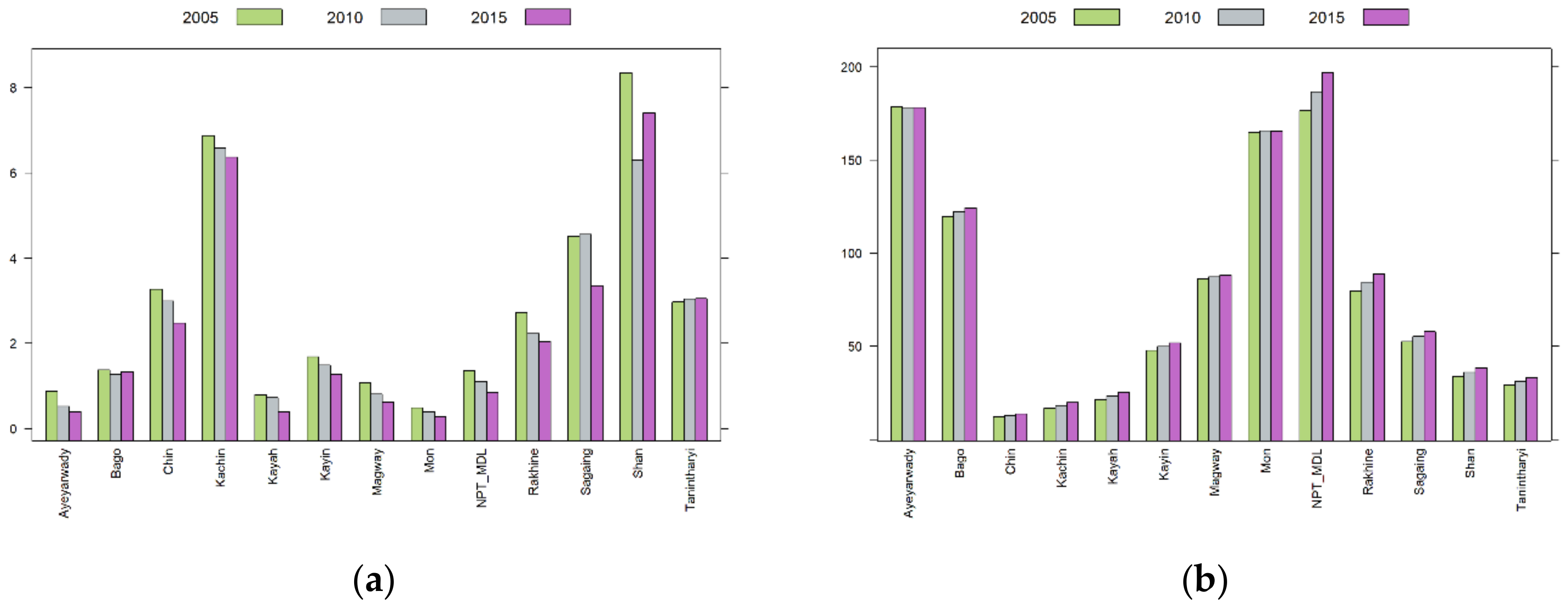
First, forest area was the response variable in this regression. The dataset for three different years—2005, 2010, and 2015—was contributed by the Forest Department (FD) of Myanmar and the information collected for those years were represented as national datasets. The FD assesses the country’s forest cover in five-year intervals in order to be in line with the reporting time required by the global Forest Resource Assessment (FRA) of the Food and Agriculture Organization (FAO). In addition, the term forest area is defined in the 2015 FRA as “Land spanning more than 0.5 hectares with trees higher than 5 m and a canopy cover of more than 10 percent, or trees able to reach these thresholds in situ. It does not include land that is predominantly under agricultural or urban land use [34].” These thematic forest-cover maps were pixel-based and produced through supervised maximum-likelihood classifiers using imagery from the Landsat satellite imagery program (30 m), for the years 2005 and 2015, and using imagery from IRS (Indian Remote Sensing Satellites, 23.5 m) for the year 2010. State and regional forest areas, measured in hectare, were calculated for these three years using GIS (Geographic Information System) and administration boundaries. Before using the national datasets, we checked Global Forest Change (GFC) maps to use as an independent source of data on land cover [41]. We found that GFC was focused on the global level and possessed some limitations as to its use at the national data level. GFC gave much lower estimated forest cover change and did not fit with the observed national circumstances. Therefore, we used national datasets instead of the available global datasets. Forest area data are shown in Figure 1a. Almost all of the states and regions demonstrated deforestation from 2005 to 2010 and from 2010 to 2015 with some exceptions.
In this research, two factors, population and GDP, were considered as explanatory variables to analyze the impact of socioeconomic development on forest areas. By now, three population censuses have been conducted: in 1973, 1983, and 2014. The 2014 Myanmar Population and Housing Census provides the most reliable population data for Myanmar to date. In the 1990s and 2000s, censuses were not undertaken; however, several household-based surveys were carried out. After publishing the basic results of the population census, the Department of Population (DOP) also published thematic reports, including Thematic Reports on Mortality and Thematic Reports on Fertility and Nuptiality. The DOP later produced a Thematic Report on Population Projections of annual data through 2050 on the national level and through 2031 on the state and regional levels [42,43,44]. For the void before 2014, experts at the DOP backcast annual data by using 1983 as the base year and projected upward to 2014 by using Spectum Software. Fertility and mortality indicators used in the backcasting were sourced from the series of Fertility and Reproductive Health Surveys that were conducted in 1991, 1997, 2001, and 2007. Internal and international migration data were estimated based on the 2014 Population and Housing Census. Since the fiscal year in Myanmar ended on 31 March until 2018, the population data for the year are the data as of 1 October, the middle of the year (note: after October 2018, the new fiscal year will end on 30 September). For this research, the backcast population data by states and regions in 2005, 2010, and 2015 were obtained from the DOP. The approach used for backcasting was the same as that used in population projections. Interested readers may refer to the Thematic Report on Population Projections [44]. By dividing the total population (unit: persons) in a state or region by the land area, population density (unit: persons per km2) was obtained. Both the total population and the population density are good variables in considering the population factor, because they reflect the gross population volume and amount of population per unit area, respectively. Population density data are shown in Figure 1b. Except for the Ayeyarwady Region and Mon State, all other states and regions had an increase in their population and population density.
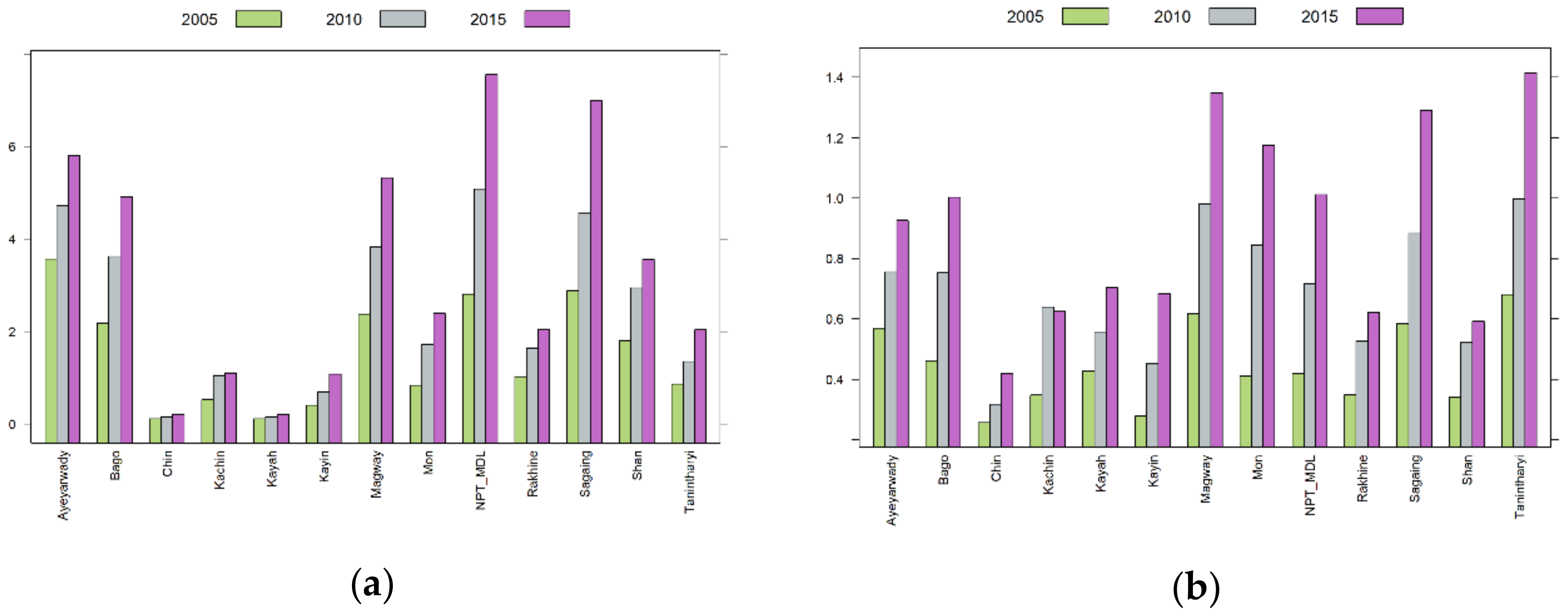
Another factor considered in this research was GDP. GDP expresses the monetary value of the final goods and services produced in a country or a region in a given period of time. Annual GDP growth rates were 8.4%, 7.0%, and 6.8% during 2013–2014 (April 2013 to March 2014), 2015–2016, and 2017–2018 fiscal years, respectively [39]. In Myanmar, GDP consists of three sectors: agriculture, industry, and services. Agriculture grows slowly. Natural disasters such as flooding and landslides damage agricultural harvests. Industry grows steadily, especially the processing and manufacturing industries, and the construction industry is developing well. The shares of GDP in these three sectors are changing. The share of the agriculture sector decreased from 46.7% in fiscal year 2005–2006 to 36.8% in fiscal year 2010–2011, to 26.8% in fiscal year 2015–2016. However, the shares of the industry and services sectors are increasing, 17.5%, 26.5%, and 34.5% for industry, and 35.8%, 36.7%, and 38.7% for the services sector, respectively, for the corresponding years. Foreign direct investment is very important for a developing country. In Myanmar, foreign investment of permitted enterprises increased from $4107 million (US) in fiscal year 2013–2014 to $9486 million (US) in 2015–2016. However, it decreased to $6649 million (US) in 2016–2017 and to $5718 million (US) in 2017–2018, corresponding to the decreases in GDP growth in 2016–2017 and 2017–2018. In the model, GDP can be expressed by total GDP (unit: million Kyats) or per capita GDP (unit: Kyats) in a state or region. Total GDP reflects the size of economic production while per capita GDP shows a country’s GDP divided by its total population and reflects the general level of wealth and prosperity per person. Both total GDP and per capita GDP are good indexes and are widely used in the analysis of deforestation issues. Therefore, these two variables were used in the model. Data of GDP by states and regions in the three fiscal years 2005–2006, 2010–2011, and 2015–2016 provided by the Ministry of Planning and Finance were used in this research [45]. GDP data were adjusted to 2010 constant prices using a World Bank GDP deflator [46]. GDP and per capita GDP are shown in Figure 2a,b, respectively. For all the states and regions, GDP and per capita GDP increased.
2.3. Method
Panel data analysis, an econometrics approach, was adopted in the research. Panel data analysis has been widely used in analyzing deforestation issues (e.g., [20,30,31,47]). For developing countries, long time-series data are usually not available. Cross-sectional data reflect the situations of various individuals at a specific point in time or time period but cannot reflect the changes among different time points or periods. Panel data are observations of the same individuals over multiple (at least two) points in time or periods. In describing the advantages of panel data analysis, Hsiao pointed out that panel data provide a large number of points, increase the degrees of freedom, reduce the collinearity among explanatory variables, and sometimes, panel data can be used to analyze some questions that cannot be analyzed by cross-sectional or time-series data [48]. In this research, data in three time periods, 2005, 2010, and 2015, were used. Myanmar has 15 states and regions: seven states, seven regions, and one Union territory. Yangon Region, where the former capital was located, has a large population, a high GDP, and not much forest. This makes it rather different from other states and regions, therefore, it was excluded from the model. Nay Pyi Taw Union Territory, the new capital, was separated from Mandalay Region in 2006. Due to data availability, Nay Pyi Taw and Mandalay are combined as one area. Thus, panel data analysis was applied to 13 areas to analyze the impacts of socioeconomic development on forest areas in the Union.
A linear regression model was assumed, and a common linear regression model can be postulated as [48]
where Yit is a response variable, αit is the intercept that varies across i and t, β’it are regression slope coefficients that vary across i and t, Xit are exogenous variables, and uit is the error term. In this research, a panel of data from 13 areas in three years were used; therefore, N = 13 and T = 3. When assuming all the intercepts and slopes are correspondingly the same across i and t, the model becomes
Yit = α*it + β’itXit + uit, i = 1, 2, …, N; t = 1, 2, …, T,
Yit = α* + β’Xit + uit.
In panel data analysis this model is called the pooled model. When assuming the regression slopes are identical across i and t and the intercepts are identical only across t but not i, the model becomes
which is called a fixed effects (FE) model. Equation (2) assumes that all individuals are homogenous; however, this rarely happens. For this research, the 13 areas have rather different characteristics, including land areas, distance to the capital, access to the border, ethnicity and culture, etc. These factors may affect forest area changes. When these variables are not included as explanatory variables, their impacts, usually called individual-specific effects, will remain in the error term; and because these variables do not change over time and their impacts probably do not change, this may give rise to a problem of serial correlation. The FE model, as shown in Equation (3), separates individual-specific effects and reflects them in intercepts in modeling for every area. When Equation (3) is compared against Equation (2), it seems that dummy variables are added for every i. The pooled model and FE model are usually estimated by the ordinary least squares method. In contrast to the pooled model, the FE model allows correlations between explanatory variables and errors.
Yit = α*i + β’Xit + uit,
When introducing a mean intercept, μ, for α*i into Equation (3), the model becomes
Yit = μ + β’Xit + αi + uit.
By further restricting the sum of αi to zero same as uit, assuming that there is no correlation between αi and uit, the model in Equation (4) is called the random effects (RE) model or the components of variance model [48]. The RE model assumes that the individual-specific errors and the overall errors are random variables drawn from a normal distribution, and are independently and identically distributed, and these error components are not correlated with the explanatory variables. Since the presence of αi, a generalized least-squares method had to be used for the RE models. In order to choose the best models—the pooled model, the FE model, or the RE model—an F-test, Breusch–Pagan test, and Hausman test were implemented [49,50].
Two factors, population and GDP, with four variables were considered. The best combination of one population variable between total population and population density and one GDP variable between total GDP and per capita GDP was chosen by the Akaike information criterion (AIC). When the assumption of identical variances of the errors across individuals is violated, the problem of heteroscedasticity can arise [51]. Therefore, the null hypothesis of homoscedasticity was tested, and robust covariance matrix estimations were provided if heteroscedasticity existed. Testing for serial correlation was not implemented because our data only have three time periods, and this should not be a problem.
After running the model, annual forest areas were forecast from 2016 to 2020 by using medium population projections and the three GDP growth scenarios. To deal with uncertainty, forecast intervals were calculated. Finally, sensitivity analysis was implemented.
3. Results
Two main results were obtained: the impact of socioeconomic factors on forest area changes were clarified and annual forest areas from 2016 through 2020 were forecast.
3.1. Fitting Models
3.1.1. Modeling and Model Selection
There are six possible combinations among the four variables: total population (POP), population density (PD), total GDP (GDP), and per capita GDP (PGDP). However, combinations of two population variables and of two GDP variables were avoided. Therefore, four combinations remained. Since the correlation coefficient between POP and GDP was 0.85 (p-value < 0.001), a combination of POP and GDP was excluded. Our models only have two explanatory variables. When they are highly correlated, it is difficult to change one variable and hold the other variable constant. Thus, the remaining three combinations were dealt with. Test results are shown in Table 1. First, according to the results in items (2) and (3), both FE and RE models are better than the pooled model at the 1% level of significance for all three combinations. According to the results in item (4), the null hypothesis that assumes the explanatory variables are uncorrelated with the specific effects was not rejected at 5% significance level in all three combinations; therefore, RE models are better than FE models. Second, as shown in item (5), the studentized Breusch–Pagan test shows that all three combinations in the model have heteroscedasticity, implying that robust covariance matrix estimations are needed in calculating standard errors and F-statistics. The results in items (6) and (7) show that RE models have a lower AIC than FE models. Among RE models, combinations 1 and 2 have lower AICs than combination 3. However, the difference between combinations 1 and 2 is 0.37, and it is hard to say which is better. Results in item (8) show that the adjusted R-squared values are from 0.20 to 0.28 for RE models, and combination 2 shows the highest value. Lastly, results of F-statistics and their p-values in item (9) show that all the RE models are significant.
Results of RE models in combinations 1, 2, and 3 are shown in Table 2. Intercepts and PGDP in both models and PD in the second model had significant estimates at the 1% level. A high standard error and p-value but a low z-score for POP in model 1 failed to reject the null hypothesis that the coefficient is different from zero. The signs for PGDP, GDP, and POP are negative, implying that these variables have negative impacts on forest areas, while the impact of POP could not be detected statistically. Since all the estimators in model 2 were statistically significant and had higher adjusted R-squared values than models 1 and 3, model 2 was considered the best model in this research.
3.1.2. Validation of Model Estimations
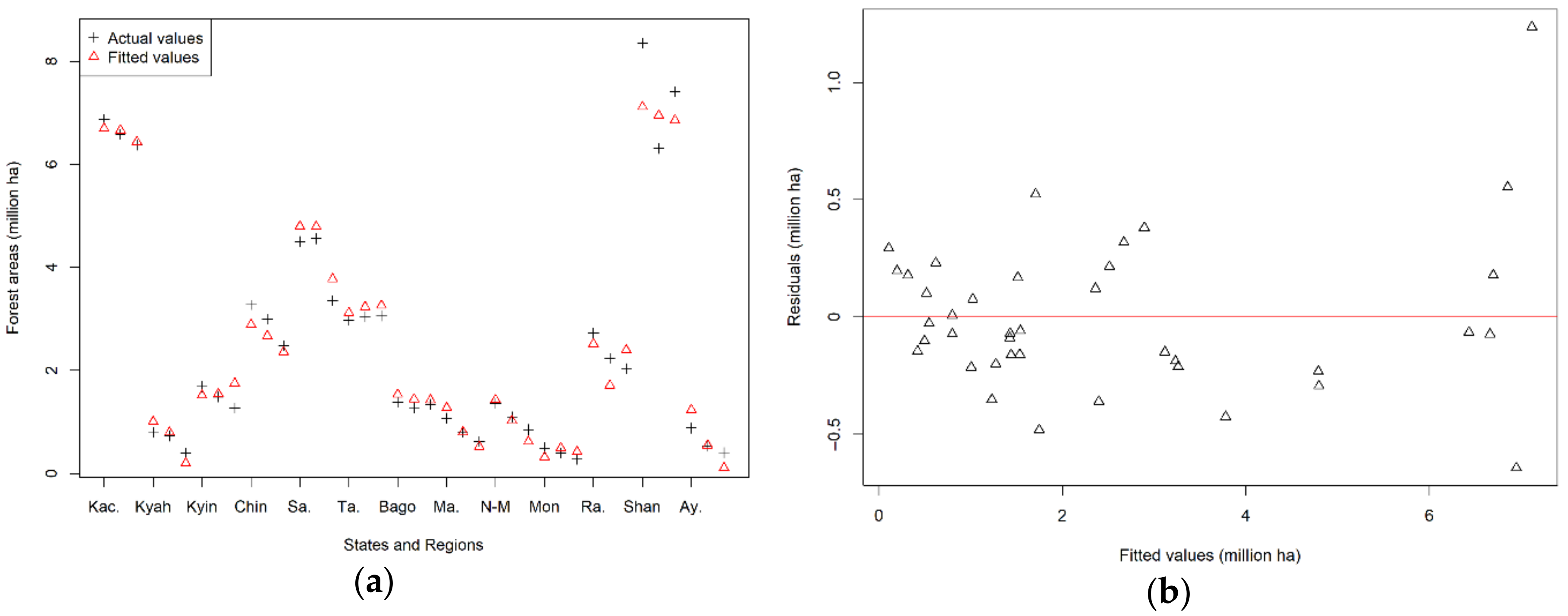
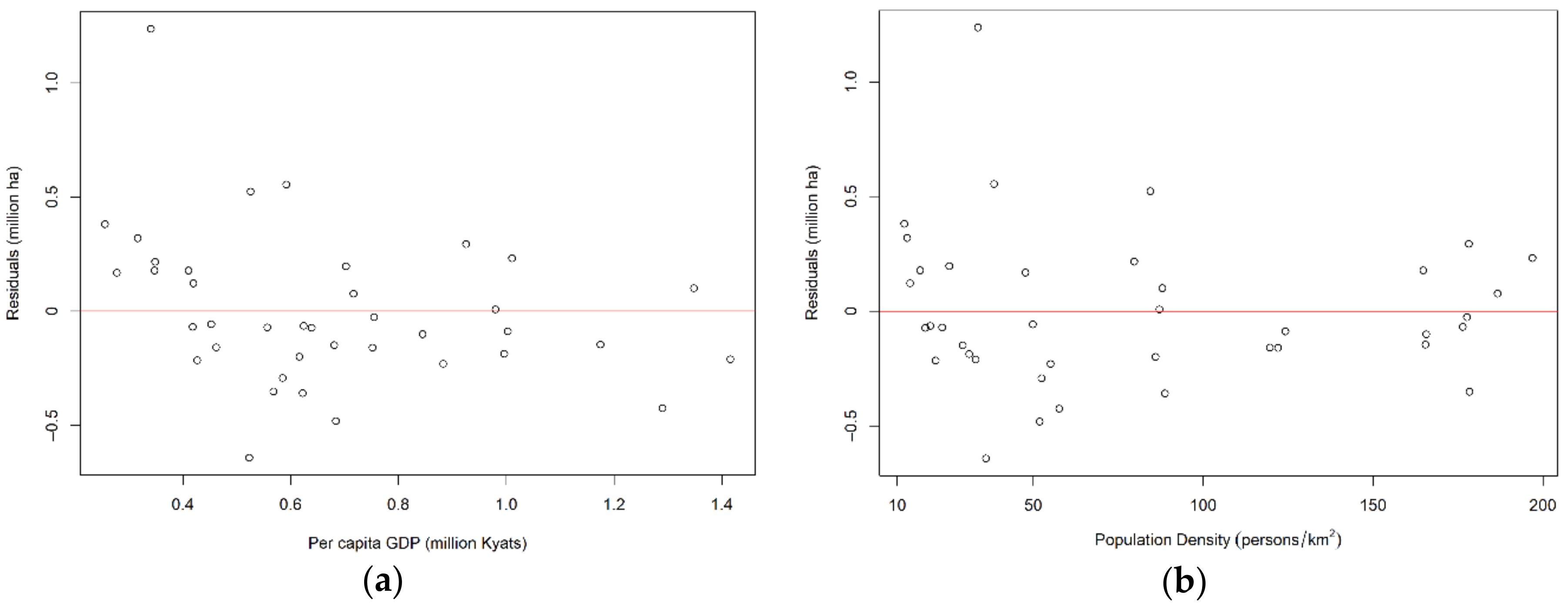
After obtaining the best model in Section 3.1.1, which showed that model 2 is a good model, we validated the model visually as depicted in Figure 3 and Figure 4. In Figure 3a, Kachin was abbreviated as Kac., Kayah as Kyah, Kayin as Kyin, Sagaing as Sa., Tanintharyi as Ta., Magway as Ma., Nay Pyi Taw and Mandalay as N-M, Rakhine as Ra., and Ayeyarwady as Ay. Figure 3a shows that the fitted values are very close to the actual values in most cases. The fitted values in Shan State show larger errors, which may be caused by errors in the original data. Figure 3b shows that the residuals are well scattered around the horizontal line of zero and that no obvious trend is observable. Comparisons of residuals versus two explanatory variables are shown in Figure 4a,b. Similar to the results in Figure 3b, some values show high deviations, but neither of these figures show any obvious pattern in the residuals. In order to examine the existence of endogeneity, we also calculated correlation coefficients among the residuals and two explanatory variables. The correlation coefficient for residuals and PGDP was −0.314 (p-value = 0.052), and the 95% confidence interval was calculated as (−0.573, 0.002). Our calculation showed a weak correlation of −0.314 that was not significant at 5% level, and the range of the 95% confidence interval shows that a zero correlation cannot be denied. As for PD, it was −0.062 (p-value = 0.706). Therefore, endogeneity was not detected, and the model is considered to fit the data well.
3.2. Forecasting Forest Areas
3.2.1. Forecasting Using the RE Model
Modeling forest area using PD and per capita GDP has shown that these two variables gave statistically significant negative impacts on forest areas. This model was used in forecasting annual forest areas from 2016 to 2020. The model reflects that when the explanatory variables change, the response variable will also change. When the values of the explanatory variables for the coming years were given, the fitted values of the responses for the corresponding years become the projections or forecasts.
By rewriting Equation (4) and setting the future values of the explanatory variables as X0, where X0 is two vectors, and the value of Y0, where Y0 is one vector associated with X0, the forecast values of the response variable can be obtained by
Y0 = β’X0 + ε0.
By applying to the Gauss–Markov theorem, we obtained the fitted values or forecasts of
which is the minimum variance linear unbiased estimator of E[Y0] [56].
Yhat0 = b’X0,
The two vectors of X0 are the PD vector and the per capita GDP vector. In order to forecast annual forest areas from 2016 to 2020, these two vectors were needed for those years. Fortunately, the DOP publishes the population projections for states and regions through 2031 based on the 2014 Myanmar Population and Housing Census. Three variant projections, low, medium, and high, were provided for the Union level, based on assumptions on the future trends in fertility, mortality, and internal and international migration. The growth rates of the Union population were projected as declining steadily, from about 9 per 1000 in 2015 to about 3 per 1000 in 2050 for medium projections. The growth rates of the population for states/regions were also projected to decline, but different states/regions had different growth rates. In addition, for states/regions, only medium variant levels of projections were provided. The data for the total population by states and regions were used to calculate PD and were taken as inputs in forecasting.
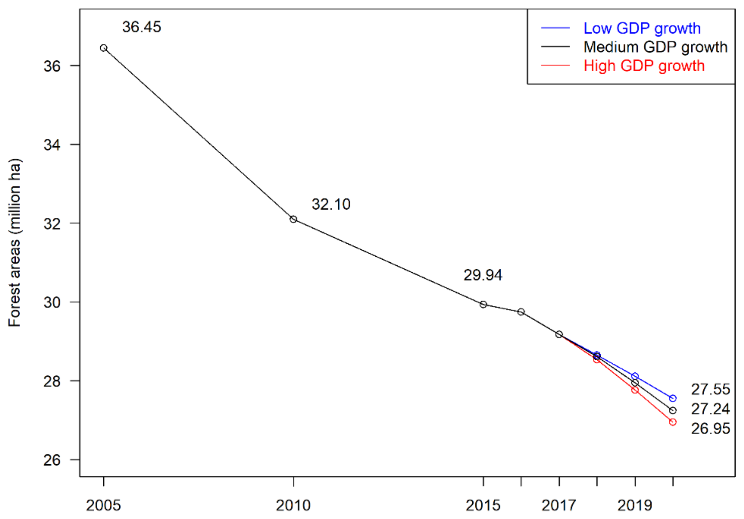
Per capita GDP data for states/regions from 2016 to 2020 were also needed in forecasting. Myanmar published annual per capita GDP growth rates for the Union, but not for states and regions. For the past five years, the annual per capita GDP growth rates were 7.3%, 6.3%, 6.1%, 4.9%, and 5.8% for 2013–2014, 2014–2015, 2015–2016, 2016–2017, and 2017–2018, respectively [39]. The last two growth rates were used directly for 2016 and 2017 forecasting. In 2018, Myanmar changed its fiscal year from 1 April–31 March to 1 October–30 September. After fiscal year 2017–2018 finished in March 2018, there was a six-month period from April 2018 to September 2018 that had to be accounted for. The World Bank projected the GDP growth rates as 6.4% in this period, 6.5% in fiscal year 2018–2019 fiscal year (from October 2018 to September 2019), and 6.7% in fiscal year 2020–2021 (from October 2020 to September 2021) [57]. For our research objectives and data consistency, fiscal years 2018–2019, 2019–2020, and 2020–2021 were made comparable to previous years by setting them to end in March. Then three scenarios were setup: low, medium, and high. The lowest level from the past five years, 4.9%, was taken as the annual per capita GDP growth rate in the low scenario for these three years. Considering the population growth and GDP growth projected by the World Bank, 5.4%, 5.5%, and 5.7% were assumed for the medium scenario; the second highest level in the most recent five years, 6.3%, became that of the high scenario. Since there are no data for states and regions, the same growth rates were assumed for all states and regions. By using medium-level population projections and the three scenarios of per capita GDP, annual forest areas were forecast for the years from 2016 through 2020. Yangon Region was not included in the panel data analysis; however, in order to forecast all the forest areas in Myanmar, the forest area in Yangon in 2015 was added to every year by assuming that there was no deforestation or afforestation in Yangon from 2016 to 2020. The results are shown in Table 3. Based on the forecasting results, deforestation areas were also calculated (see Table 4). The results show that high GDP growth caused higher deforestation. Since 2017, the forecast deforestation areas were higher than 0.50 million hectare. In 2016, deforestation was lower than in other years. This was not only because of the low per capita GDP growth rate, but also because of the residuals in the model in 2015. For the years from 2017 to 2020, deforestation was projected as increasing because of increasing per capita GDP. The deforestation in 2010 to 2015 was lower than during the period from 2005 to 2010. However, deforestation was projected as increasing again. This is shown visually in Figure 5.
3.2.2. Forecast Intervals
Uncertainty always exits. First, errors in the forecasting results come from the original data. The data used in this research are the best data that could be obtained; however, errors still exist. Calculating errors in the original data are beyond this research. As for the models, errors can come from the specification of parameters of the model and the error term in the model. The forecast variance from the specified model can be shown as follows [56]:
Var[e0] = Var[Y0 − Yhat0] = σ2 + Var[(β − b)’X0].
The first component on the right side shows the forecast variance from the error term, the second component shows the source from the estimation of parameters. Based on Equation (7), the forecast interval (FI) can be calculated as follows:
where se is the standard error, tλ/2 is the value from the t distribution that is exceeded with probability λ, the confidence level. The values of t are about 1.28 and 1.96 at the 80% and 95% confidence intervals, respectively. Table 5 shows FIs with lower and upper bounds at 80% and 95% probability levels. The FI here implies that the true value of the forest areas was expected to lie between the lower bound and upper bound with 80% or 95% confidence. A wide range is shown in Table 5. The forecasts in Table 3 are point forecasts, the means of the response variable under the conditions of the explanatory variables. A wide FI means uncertainty is large. This result was obtained probably because of the small size of the data and the heterogeneous characteristics of states and regions.
FI = Yhat0 ± tλ/2 se(e0),
3.2.3. Sensitivity Analysis
Table 3 and Table 4 show the forecasting results using the three GDP scenarios and the medium level of the population projections. The DOP does not provide low- and high-level projections for states and regions like it does for the Union. Here, the low variant and high variant of the projected population growth rates from 2016 to 2020 by states and regions were obtained in adjusting the populations of the states and regions by the ratios of low variant to medium variant and high variant to medium variant in Union levels in corresponding years. The medium projected growth for the Union for the years 2016 to 2020 is 0.89%, 0.89%, 0.88%, 0.88%, and 0.87%. For the low variant they are 0.87%, 0.87%, 0.86%, 0.84%, and 0.83%, and for the high variant they are 0.91%, 0.92%, 0.92%, 0.93%, and 0.93%. Ratios were calculated based on these growth rates in corresponding years. Based on the ratios, low and high variants for the populations in the states and regions were calculated. The forecasts are shown in Table 6. The differences between the forecasts for low and high population growth compared with that of medium growth are only 9000 and 14,000 hectares in 2020, respectively. The Union population in the low variant in 2020 is projected by the DOP as 54,763,768, that of the medium variant is 54,817,919, and that of the high variant is 54,903,645. Since the differences among population projections are not large, their projected impacts are also not large.
4. Discussion
The random effects models for all three combinations are significant overall as shown by the F-test results (Table 2). These three models show that GDP, per capita GDP, and PD indicated negative impacts on forest areas. Per capita GDP and PD variables had different, but close, coefficients in different models, proving that these models were well specified. Total population was not detected as a significant variable, even though it had a negative slope, probably because of the sample size. Validations of model estimations show the best model as acceptable.
Forecasting is a natural extension after modeling. However, very little forecast research on forest resources was found. In forecasting forest areas, explanatory variables are forecast first. Fortunately, the DOP provided population projections for states and regions. The World Bank publishes economic forecasts for Myanmar, and these forecasts were used as references for setting up GDP conditions. Medium scenarios were set as 4.9%, 5.8%, 5.4%, 5.5%, and 5.7% for per capita GDP growth rates for the years from 2016 to 2020. The low scenario was 4.9% annually, and the high scenario was 6.3% annually for the last three years while keeping the first two years the same as the medium scenario. As a result of these changes, the differences in forecasts of forest areas in 2020 will be approximately 300,000 ha between medium and low, and between medium and high scenarios. Forecasting results show increasing deforestation with increasing per capita GDP.
Due to uncertainty, low and high population variants were also considered in the sensitivity analysis. The differences in low, medium, and high population projection variants are small; therefore, the differences in the forecasts are also small. This does not mean that population is not an important factor. If the actual population growth is far beyond these projections, their impacts may also be larger. The scenario settings are somewhat arbitrary, and this leaves room for improvement.
This research clearly shows that the two variables, per capita GDP and PD, had significant impacts on forest areas. Higher economic development and population growth implied higher deforestation in the period from 2005 to 2015, and this relationship will probably continue for some years. Agriculture’s share of total GDP has been decreasing. Therefore, developing those sectors or sections of the economy that do not cause deforestation, such as manufacturing and the service sector, is very important to lessen the pressure on agriculture and forests.
Among the small amount of literature on forecasting forest areas, Michinaka et al. forecasted forest areas for Cambodia from 2011 through 2018 by using the provincial panel data in 2002, 2006, and 2010 [31]. The forecasts for 2014 and 2016 were, respectively, 9.94 and 9.72 million ha, but the actual forest areas were 8.99 and 8.74 million ha in the corresponding years. As a result of the deeper deforestation from 2010 to 2014, the actual forest area is lower than the forecast, and the error is 9.56% for 2014 based on the 2014 forecast. This is a large error even though the actual values are within the range of the FI at the 95% level calculated in the forecast [31]. The forecast deforestation between 2014 and 2016 is 0.22 million ha and the actual deforestation in the same period is 0.25 million ha, leading to a small error of 0.33% based on the 2014 actual forest areas. It should be noted that the actual forest areas are smaller than the forecast forest areas, which were forecast based on the data from 2002 to 2010. Like Cambodia, Myanmar is a developing country and is positioned at a transition period; therefore, greater deforestation is possible.
Myanmar has been making much progress in statistical analysis. It is publishing statistical yearbooks, including the most recent ones, Statistical Yearbooks 2015 and 2018. Household-based surveys are helpful in projecting population. However, data for states and regions are not available in many cases. Panel data analysis is a powerful approach by which short-but-wide panel data can be analyzed. It is acceptable for data to be of short duration; however, subnational or regional data are needed in the analysis of the whole country. Two factors, GDP and population, were analyzed in this research. Other factors, such as agricultural or arable land area, rural and urban population, road density, poverty rate, and employment that were used in previous research, were reviewed in the Section 1 and may also be important. If more data are available, the research may be improved.
GDP is a widely used factor in analyzing deforestation. However, there are limitations. In Myanmar, clearing forestland for farming, either subsistence farming or business farming, is an important direct driver. Many natural disasters, such as flooding and landslides, have damaged agriculture and made growth of the agricultural economy slow in Myanmar. These hazards are probably the results of deforestation. Instead of GDP, rural or arable land area may be better factors when analyzing deforestation in Myanmar.
Yangon was not dealt with in this panel data analysis. This does not mean Yangon is not important to Myanmar forestry. Economic development in Yangon attracts migrations from neighboring states and regions, even from remote areas, which may lessen the pressure of population growth on forests in those areas. In the process of economic development and population growth, Yangon may impose its role on tree plantation and give influence to other states and regions, such as providing job opportunities in industry and service sector. In this research, Nay Pyi Taw Union Territory was combined with the Mandalay Region because of data availability. If the data were available, these regions should be separated because they are different areas with different characteristics.
In recent years, Myanmar has made many efforts in forest conservation and sustainable forest management. The Myanmar Reforestation and Rehabilitation Programme (MRRP) is one of them. MRRP is a national level, long-term program, developed to prevent deforestation and forest degradation. MRRP was designed on two project phases, 2017–2018 to 2021–2022 and 2022–2023 to 2026–2027. Myanmar also actively implements the REDD+ scheme. Myanmar became a partner country of the UN-REDD program in 2011, and the REDD+ Readiness Roadmap was completed in 2013. The country has submitted the proposed FRL and a report of the technical assessment on the FRL was published by UNFCCC. Many other policies and strategies are also being implemented, including meeting the requirement of Forest Law Enforcement, Governance, and Trade (FLEGT), the logging ban in Bago Mountain Range since 2016, land use management, and anti-corruption, and so on. These measures and policies contribute to lessening deforestation and forest degradation.
Applying forest transition theory, we found that Myanmar is in the stage of resource depletion. If we adopt the cutoff criteria of levels of forest cover and annual rate of deforestation defined by Griscom et al., Myanmar can be categorized as an MFHD country (i.e., medium forest cover (35%–50%), high rate of deforestation (0.8%–1.5%)) [58]. Due to the fact that Myanmar has a very low per capita GDP, we argue that Myanmar is positioned at the early stage of resource depletion in forest transition. Forests in Myanmar have to face pressure from the developing economy. Currently, population growth is an important underlying driver of deforestation. However, the current growth rate of the population is about 0.9%, which is around the average global level. DOP has projected that the population growth rate will slow down. Therefore, the pressure that population growth places on forests will be lessened. Of course, due to the efforts of the country and international society, forest transition may come earlier. Forest transition does not occur just as a result of the passage of time but from a combination of many factors.
In our research, the impacts of demographic and economic factors, the two underlying causes of deforestation were analyzed. Deforestation is mainly the result of human behavior due to specific socioeconomic circumstances. The roles that people play regarding forests in a country may vary when their socioeconomic circumstances change [20]. Many researchers use per capita GDP or income to reflect socioeconomic development; however, demographers have also found a population growth transition during the process of socioeconomic development in many countries and regions and have proposed a population transition theory [59,60]. Population growth may show a pattern of transition from high to low and even to negative growth due to declining fertility and mortality rates. Population transition theory shows that population growth not only relates with economic development and technical progress but also has its own dynamics. Demographic development is also an important factor that has considerable impacts on society. This research analyzed the impacts of both demographic and economic factors, rather than simply focusing on economic development or the passage of time. Needless to say, the impacts of both may change, and this is why our forecasts were implemented only to 2020, an interval of five years.
In this study, a linear regression model was used. By differencing two sides, we arrived at the equation ∆forest area = β1∆PGDP + β2∆PD. Changes in per capita GDP and population density (right side) were used to explain deforestation (left side). This was based on the logic that deforestation was caused by a strong demand for forest land due to the increase in economic consumption (high per capita GDP implies high purchasing power) and population growth. However, deforestation may also contribute to the increase in GDP or per capita GDP. If this is true, a problem of endogeneity exists, and the estimates of parameters could be biased. In Myanmar, the contribution of deforestation to GDP cannot be denied. However, this contribution is declining. As explained earlier, clearing land for farming is an important direct driver of deforestation, however, the share of the agricultural sector as a portion of GDP is getting smaller and smaller. The industrial and service sector are developing much faster. In the past, mining had been found to be a driver of deforestation, but it only creates minor impacts now. Floods and landslides have damaged some agricultural harvests and made deforestation contribute less to GDP. In Section 3.1.2, model validation was implemented and endogeneity was not detected. Therefore, we conclude that the estimates of our parameters were consistent. When new data are obtained, the model may be improved.
As explained in the FRL report, Myanmar used a sample-based approach to estimate deforestation between the years of 2005 and 2015 [1]. Based on a stratified random sample design, 11,284 forest inventory plot data were collected from all over the country. Myanmar estimated and proposed the bias-corrected annual gross deforestation at about 428,984 ha during the reference period of 2005–2015 by following the Intergovernmental Panel on Climate Change (IPCC) guidelines and the Global Forest Observations Initiative (GFOI) methods. Gutman and Aguilar-Amuchastegui [61] summarized three types of approaches to the establishment of forest reference emission levels (FREL/FRLs): (1) the strictly historical approach, (2) the adjusted historical approach, and (3) simulation models. By December 2019, 40 countries among 61 partner countries have submitted their proposed FREL/FRLs [62]. Most countries used a historical average as their FREL/FRLs, and few countries made linear projections of historical change [63]. Myanmar is an example of the first approach. However, this research showed that deforestation from 2017 to 2020 will be higher than 428,984 ha. Therefore, we suggest adjusting the estimated amount upward and adopting the second approach. As for the third approach, utilization is still difficult due to uncertainty.
5. Conclusions
Economic development and population growth, expressed as total GDP, per capita GDP, and population density in this research impose significant pressure on forest areas in Myanmar. Forecasting results show that annual deforestation will exceed 0.5 million hectares and increase as the economy develops and the population grows. Faster economic growth may imply higher deforestation in the near future. Myanmar is in the process of a political and economic transition. Currently, there is one-digit GDP growth in Myanmar; but in the future two-digit economic growth is not impossible. This research implies the direction and magnitude of the adjustment to the proposed FRL by considering the national circumstances of economic development and population growth. Therefore, the results of this research may be useful in improving the FRL in REDD+ in Myanmar.
Author Contributions
Conceptualization, T.M. and T.S.; methodology, T.M.; software, T.M.; validation, T.M., T.N.O., and M.S.M.; formal analysis, T.M.; investigation, E.E.S.H., T.M., and T.N.O.; data curation, T.M. and E.E.S.H.; writing—original draft preparation, T.M. and M.S.M.; writing—review and editing, T.M., E.E.S.H., and T.N.O.; visualization, T.M.; supervision, T.S.; project administration, T.S.; funding acquisition, T.S. and T.M. All authors have read and agreed to the published version of the manuscript.
Funding
This research was conducted in “the project to support activities for promoting REDD+ by private companies and non-governmental organizations” using subsidy from Forestry Agency, Japan.
Acknowledgments
The authors thank U Kan Shein on GDP data, Khaing Khaing Soe on population data, Gen Takao on design of the research, Inkyin Khaine, Khin thida Htun, Kyi Phyu Aung, Chan Myae Aung, and other staff in the Forest Research Institute, Forest Department, and other Ministries and Departments on data collection and field trips in Myanmar.
Conflicts of Interest
The authors declare no conflicts of interest.
References
- Ministry of Natural Resources and Environmental Conservation (MONREC), Myanmar. Forest Reference Level (FRL) of Myanmar. Nay Pyi Taw, Myanmar, 2018. Available online: https://redd.unfccc.int/files/revised-myanmar_frl_submission_to_unfccc_webposted.pdf (accessed on 18 October 2019).
- United Nations Framework Convention on Climate Change (UNFCCC). Report of the Technical Assessment of the Proposed Forest Reference Level of Myanmar Submitted in 2018; UNFCCC: Bonn, Germany, 2019; Available online: https://unfccc.int/sites/default/files/resource/tar2018_MMR.pdf (accessed on 18 October 2019).
- Ministry of Natural Resources and Environmental Conservation (MONREC), Myanmar, REDD+ Myanamr, UN-REDD. Drivers of deforestation and forest degradation in Myanmar. Nay Pyi Taw, Myanmar, 2017. Available online: http://www.myanmar-redd.org/wp-content/uploads/2017/10/Myanmar-Drivers-Report-final_Eng-Version.pdf (accessed on 18 October 2019).
- Mather, A.S. Global Forest Resources; Belhaven Press, a Division of Printer Publishers: London, UK, 1990. [Google Scholar]
- Mather, A.S. The forest transition. Area 1992, 24, 367–379. [Google Scholar]
- Kothke, M.; Leischaner, B.; Elsasser, P. Uniform global deforestation patterns—An empirical analysis. For. Policy Econ. 2013, 28, 23–37. [Google Scholar] [CrossRef]
- Ashraf, J.; Pandey, R.; Jong, W. Assessment of bio-physical, social and economic drivers for forest transition in Asia-Pacific region. For. Policy Econ. 2017, 76, 35–44. [Google Scholar] [CrossRef]
- Barbier, E.B.; Delacote, P.; Wolfersberger, J. The economic analysis of the forest transition: A review. J. For. Econ. 2017, 27, 10–17. [Google Scholar] [CrossRef]
- Angelsen, A. Forest Cover Change in Space and Time: Combining the Von Thunen and Forest Transition Theories. In World Bank Policy Research Working Paper # 4117; World Bank: Washington, DC, USA, 2007; p. 43. Available online: https://ssrn.com/abstract=959055 (accessed on 6 April 2018).
- Angelsen, A. How do we set the reference levels for REDD payments? In Moving Ahead with REDD: Issues, Options and Implications; Angelsen, A., Ed.; CIFOR: Bogor, Indonesia, 2008; Available online: https://www.cifor.org/library/4572/ (accessed on 5 November 2019).
- Rowcroft, P. Frontiers of change: The reasons behind land-use change in the Mekong Basin. AMBIO 2008, 37, 213–218. [Google Scholar] [CrossRef]
- Basu, A.; Nayak, N.C. Underlying causes of forest cover change in Odisha, India. For. Policy Econ. 2011, 13, 563–569. [Google Scholar] [CrossRef]
- Buongiorno, J.; Zhu, S. Using the Global Forest Products Model (GFPM version 2016 with BPMPD). In Staff Paper Series #85; Department of Forest and Wildlife Ecology, University of Wisconsin-Madison: Madison, WI, USA, 2016. Available online: https://www.srs.fs.usda.gov/pubs/ja/2016/ja_2016_buongiorno_003.pdf (accessed on 24 October 2019).
- Panayotou, T. Empirical tests and policy analysis of environmental degradation at different stages of economic development. In Working Paper WP238; Technology Publishing and Employment Programme, International Labour Organization: Geneva, Switzerland, 1993; Available online: http://www.ilo.org/public/libdoc/ilo/1993/93B09_31_engl.pdf (accessed on 27 November 2017).
- Culas, R.J. REDD and forest transition: Tunnelling through the environmental Kuxnet curve. Ecol. Econ. 2012, 79, 44–51. [Google Scholar] [CrossRef]
- Bhattarai, M.; Hammig, M. Institutions and the environmental Kuznets curve for deforestation: A crosscountry analysis for Latin America, Africa and Asia. World Dev. 2001, 29, 995–1010. [Google Scholar] [CrossRef]
- Choumert, J.; Motel, P.C.; Dakpo, H.K. Is the Environmental Kuznets Curve for deforestation a threatened theory? A meta-analysis of the literature. Ecol. Econ. 2013, 90, 19–28. [Google Scholar] [CrossRef]
- Michinaka, T. Approximating forest resource dynamics in Peninsular Malaysia using parametric and nonparametric models, and its implications for establishing forest reference (emission) levels under REDD+. Land 2018, 7, 70. [Google Scholar] [CrossRef] [Green Version]
- Nagata, S.; Inoue, M.; Oka, H. The Utility and Regeneration of Forest Resources; Rural Culture Association: Tokyo, Japan, 1994. (In Japanese) [Google Scholar]
- Michinaka, T.; Miyamoto, M. Forests and human development: An analysis of the socioeconomic factors affecting global forest area change. J. For. Plan. 2013, 18, 141–150. [Google Scholar] [CrossRef]
- Mather, A.S.; Needle, C.L. The forest transition: A theoretical basis. Area 1998, 30, 117–124. Available online: https://0-www-jstor-org.brum.beds.ac.uk/stable/20003865 (accessed on 5 November 2019). [CrossRef]
- Kimmins, H.; Blanco, J.A.; Brad, B.; Welham, C.; Scoullar, K. Forecasting Forest Futures: A Hybrid. Modelling Approach to the Assessment of Sustainability of Forest Ecosystems and Their Values; Earthscan Publications: London, UK, 2010. [Google Scholar]
- Vieilledent, G.; Grinand, C.; Vaudry, R. Forecasting deforestation and carbon emissions in tropical developing countries facing demographic expansion: A case study in Madagascar. Ecol. Evol. 2013, 3, 1702–1716. [Google Scholar] [CrossRef] [PubMed] [Green Version]
- Jha, S.; Bawa, K.S. Population growth, human development, and deforestation in biodiversity hotspots. Conserv. Biol. 2006, 20, 906–912. [Google Scholar] [CrossRef] [PubMed]
- Baptista, S.R.; Rudel, T.K. A re-emerging Atlantic forest? Urbanization, industrialization and the forest transition in Santa Catarina, southern Brazil. Environ. Conserv. 2006, 33, 195–202. [Google Scholar] [CrossRef]
- Miyamoto, M. Forest conversion to rubber around Sumatran villages in Indonesia: Comparing the impacts of road construction, transmigration projects and population. For. Policy Econ. 2006, 9, 1–12. [Google Scholar] [CrossRef]
- Rudel, T.K. Is there a forest transition? Deforestation, reforestation, and development. Rural Sociol. 1998, 63, 533–552. [Google Scholar] [CrossRef]
- Kok, K. The role of population in understanding Honduran land use patterns. J. Environ. Manag. 2004, 72, 73–89. [Google Scholar] [CrossRef]
- Top, N.; Mizoue, N.; Ito, S.; Kai, S.; Nakao, T.; Ty, S. Effects of population density on forest structure and species richness and diversity of trees in Kampong Thom Province, Cambodia. Biodivers. Conserv. 2009, 18, 717–738. [Google Scholar] [CrossRef]
- Foster, A.; Rosenzweig, M.; Behrman, J.R. Population Growth, Income Growth and Deforestation: Management of Village Common Land in India. In PIER Working Paper 97-037; Penn Pharmaceuticals (Limited Company) Institute for Economic Research, University of Pennsylvania: Philadelphia, PA, USA, 1997; Available online: https://economics.sas.upenn.edu/sites/default/files/filevault/working-papers/97-037.pdf (accessed on 29 October 2019).
- Michinaka, T.; Matsumoto, M.; Miyamoto, M.; Yokota, Y.; Sokh, H.; Lao, S.; Tsukada, N.; Matsuura, T.; Ma, V. Forecasting forest areas and carbon stocks in Cambodia based on socioeconomic factors. Int. Rev. 2015, 17, 66–75. [Google Scholar] [CrossRef]
- Miyamoto, M.; Parid, M.M.; Aini, Z.N.; Michinaka, T. Proximate and underlying causes of forest cover change in Peninsular Malaysia. For. Policy Econ. 2014, 44, 18–25. [Google Scholar] [CrossRef] [Green Version]
- Bae, J.S.; Joo, R.W.; Kim, Y.S. Forest transition in South Korea: Reality, path and drivers. Land Use Policy 2012, 29, 198–207. [Google Scholar] [CrossRef]
- Food and Agriculture Organization (FAO). Global Forest Resources Assessment 2015 (FRA 2015); FAO, UN: Rome, Italy, 2015; Available online: http://www.fao.org/forest-resources-assessment/past-assessments/fra-2015/en/ (accessed on 25 October 2019).
- Leimgruber, P.; Kelly, D.; Steininger, M.; Brunner, J.; Muller, T.; Songer, M. Forest cover change patterns in Myanmar (Burma) 1990–2000. Environ. Conserv. 2005, 32, 356–364. [Google Scholar] [CrossRef] [Green Version]
- Mon, M.S.; Kajisa, T.; Mizoue, N.; Yoshida, S. Factors affecting deforestation in Paunglaung watershed, Myanamr using remote sensing and GIS. J. For. Plan. 2009, 14, 7–16. [Google Scholar] [CrossRef]
- Mon, M.S.; Mizoue, N.; Htun, N.Z.; Kajisa, T.; Yoshida, S. Factors affecting deforestation and forest degradation in selectively logged production forest: A case study in Myanmar. For. Ecol. Manag. 2012, 267, 190–198. [Google Scholar] [CrossRef]
- Win, Z.C.; Mizoue, N.; Ota, T.; Wang, G.; Innes, J.L.; Kajisa, T.; Yoshida, S. Spatial and temporal patterns of illegal logging in selectively logged production forest: A case study in Yedashe, Myanmar. J. For. Plan. 2018, 23, 15–25. [Google Scholar] [CrossRef]
- Central Statistical Organization (CSO); Ministry of Planning and Finance, Myanmar. Myanmar Statistical Yearbook 2018; Central Statistical Organization, Ministry of Planning and Finance: Nay Pyi Taw, Myanmar, 2018.
- Department of Population (DOP); Ministry of Immigration and Population, Myanmar. The 2014 Myanmar Population and Housing Census: The Union Report, Census Report Volume 2; Department of Population, Ministry of Labour, Immigration and Population: Nay Pyi Taw, Myanmar, 2015. Available online: https://myanmar.unfpa.org/en/publications/union-report-volume-2-main-census-report (accessed on 2 February 2016).
- Hansen, M.C.; Potapov, P.V.; Moore, R.; Hancher, M.; Turubanova, S.A.; Tyukavina, A.; Thau, D.; Stehman, S.V.; Goetz, S.J.; Loveland, T.R.; et al. High-Resolution Global Maps of 21st-Century Forest Cover Change. Science 2013, 342, 850–853. [Google Scholar] [CrossRef] [Green Version]
- Department of Population (DOP). The 2014 Myanmar Population and Housing Census, Thematic Report on Mortality, Census Report Volume 4-B; Department of Population, Ministry of Labour, Immigration and Population: Nay Pyi Taw, Myanmar, 2016. Available online: https://myanmar.unfpa.org/en/publications/thematic-report-mortality (accessed on 28 October 2019).
- Department of Population (DOP). The 2014 Myanmar Population and Housing Census, Thematic Report on Fertility and Nuptiality, Census Report Volume 4-A; Department of Population, Ministry of Labour, Immigration and Population: Nay Pyi Taw, Myanmar, 2016. Available online: https://myanmar.unfpa.org/en/publications/thematic-report-fertility-and-nuptiality (accessed on 28 October 2019).
- Department of Population (DOP). The 2014 Myanmar Population and Housing Census, Thematic Report on Population Projections for the Union of Myanmar, States/Regions, Rural and Urban. Areas, 2014–2050, Census Report Volume 4-F; Department of Population, Ministry of Labour, Immigration and Population: Nay Pyi Taw, Myanmar, 2017. Available online: https://myanmar.unfpa.org/en/publications/thematic-report-population-projections (accessed on 25 April 2017).
- Agriculture, Livestock and Fishery; Forestry Sector, Ministry of Planning and Finance, Myanmar: Nay Pyi Taw, Myanmar, 2019.
- World Bank. GDP Deflator. Available online: https://data.worldbank.org/indicator/NY.GDP.DEFL.ZS?end=2018&start=2018&view=map (accessed on 25 February 2019).
- Hargrave, J.; Kis-Katos, K. Economic Causes of Deforestation in the Brazilian Amazon: A Panel Data Analysis for the 2000s. Environ. Resour. Econ. 2013, 54, 471–494. [Google Scholar] [CrossRef] [Green Version]
- Hsiao, C. Analysis of Panel Data, 2nd ed.; Cambridge University Press: Cambridge, UK, 2003. [Google Scholar]
- Breusch, T.S.; Pagan, A.R. The Lagrange multiplier test and its applications to model specification in econometrics. Rev. Econ. Stud. 1980, 47, 239–254. [Google Scholar] [CrossRef]
- Hausman, J. Specification tests in econometrics. Econometrica 1978, 46, 1251–1271. [Google Scholar] [CrossRef] [Green Version]
- Breusch, T.S.; Pagan, A.R.; Simple, A. A Simple Test for heteroscedasticity and random coefficient variation. Econometrica 1979, 47, 1287–1294. [Google Scholar] [CrossRef]
- R Core Team. A Language and Environment for Statistical Computing; R Foundation for Statistical Computing: Vienna, Austria, 2019; Available online: www.R-project.org (accessed on 5 November 2019).
- Zeileis, A.; Hothorn, T. Diagnostic checking in regression relationships. R. News 2002, 2, 7–10. [Google Scholar]
- Croissant, Y.; Millo, G. Panel Data Econometrics in R. The plm Package. J. Stat. Softw. 2008, 27, 1–43. [Google Scholar] [CrossRef] [Green Version]
- Zeileis, A. Econometric computing with HC and HAC covariance matrix estimators. J. Stat. Softw. 2004, 11, 1–17. [Google Scholar] [CrossRef]
- Greene, W.H. Econometric Analysis, 4th ed.; Prestice Hall International Editions: Upper Saddle River, NJ, USA, 2000; p. 1004. [Google Scholar]
- World Bank. Myanmar Economic Monitor June 2019. Available online: https://www.worldbank.org/en/country/myanmar/publication/myanmar-economic-monitor-reforms-building-momentum-for-growth (accessed on 5 November 2019).
- Griscom, B.; Shoch, D.; Stanley, B.; Cortez, R.; Virgilio, N. Sensitivity of amounts and distribution of tropical forest carbon credits depending on baseline rules. Environ. Sci. Policy 2009, 12, 897–911. [Google Scholar] [CrossRef]
- Myrskylä, M.; Kohler, H.; Billari, F. Advances in development reverse fertility declines. Nature 2009, 460, 741–743. [Google Scholar] [CrossRef] [PubMed]
- Galor, O. The demographic transition: Causes and consequences. Cliometrica 2012, 6, 1–28. [Google Scholar] [CrossRef] [Green Version]
- Gutman, P.; Aguilar-Amuchastegui, N. Reference Levels and Payments for REDD+: Lessons from the Recent Guyana-Norway Agreement. World Wildlife Fund USA, 2012. Available online: http://assets.panda.org/downloads/rls_and_payments_for_redd__lessons.pdf (accessed on 24 May 2012).
- UN-REDD Programme. Submissions. Available online: https://redd.unfccc.int/submissions.html?topic=6 (accessed on 17 December 2019).
- Neeff, T.; Maniatis, D.; Lee, D.; Mertens, E.; Jonckheere, I.; Perez, J.G.; DeValue, K.; Birigazzi, L.; Sandker, M.; Condor, R. From Reference Levels to Results Reporting: REDD+ under the UNFCCC. In Forests and Climate Change Working Paper 15; Food and Agriculture Organization (FAO): Rome, Italy, 2017; Available online: http://www.fao.org/3/a-i7163e.pdf (accessed on 19 April 2018).
Figure 1.
Bar plot: (a) Forest areas by state and region (unit: million ha). (b) Population density by state and region (unit: persons per km2).
Figure 1.
Bar plot: (a) Forest areas by state and region (unit: million ha). (b) Population density by state and region (unit: persons per km2).

Figure 2.
Bar plot: (a) Gross domestic product (GDP) by states and region (unit: 1012 Kyats). (b) Per capita GDP by state and region (unit: million Kyats).
Figure 2.
Bar plot: (a) Gross domestic product (GDP) by states and region (unit: 1012 Kyats). (b) Per capita GDP by state and region (unit: million Kyats).

Figure 3.
Visual model validation: (a) Fitted values versus actual values; (b) residuals versus fitted values. Kac.: Kachin; Kyah: Kayah; Kyin: Kayin; Sa.: Sagaing; Ta.: Tanintharyi; Ma.: Magway; N-M: Nay Pyi Taw and Mandalay; Ra.: Rakhine; Ay.: Ayeyarwady.
Figure 3.
Visual model validation: (a) Fitted values versus actual values; (b) residuals versus fitted values. Kac.: Kachin; Kyah: Kayah; Kyin: Kayin; Sa.: Sagaing; Ta.: Tanintharyi; Ma.: Magway; N-M: Nay Pyi Taw and Mandalay; Ra.: Rakhine; Ay.: Ayeyarwady.

Figure 4.
Visual model validation: (a) residuals versus PGDP; (b) residuals versus PD.

Figure 5.
Forecasts of three GDP scenarios.


Table 1.
Testing results and model statistics.
| Items | Combination 1 | Combination 2 | Combination 3 |
|---|---|---|---|
| PGDP + POP | PGDP + PD | GDP + PD |
| p-value < 0.001 | p-value < 0.001 | p-value < 0.001 |
| p-value < 0.001 | p-value < 0.001 | p-value < 0.001 |
| p-value = 0.256 | p-value = 0.996 | p-value = 0.114 |
| p-value = 0.041 | p-value = 0.042 | p-value = 0.045 |
| 1114.06 | 1118.05 | 1117.15 |
| 1.109.29 | 1109.66 | 1112.64 |
| 0.20 | 0.28 | 0.26 |
| 22.520 (p-value < 0.001) | 18.416 (p-value < 0.001) | 13.732 (p-value = 0.001) |
1 Results in (9) were calculated based on robust covariance matrix estimations. PGDP: per capita gross domestic product; POP: total population; GDP: gross domestic product; PD: population density; FE: fixed effects model; RE: random effects model; AIC: Akaike information criterion.
Table 2.
Model estimations.
| Model | Variables | Estimates | Standard Errors 1 | z-Values 1 | p-Values 1 |
|---|---|---|---|---|---|
| 1 | Intercept | 3732,500 | 863,070 | 4.325 | 0.000 |
| PGDP (Kyat) | −0.758 | 0.268 | −2.820 | 0.005 | |
| POP (persons) | −0.210 | 0.157 | −1.340 | 0.180 | |
| 2 | Intercept | 4629,564 | 989,760 | 4.678 | 0.000 |
| PGDP (Kyat) | −0.660 | 0.230 | −2.870 | 0.004 | |
| PD (persons/km2) | −20,562 | 6775 | −3.035 | 0.002 | |
| 3 | Intercept | 4331,700 | 1013,200 | 4.275 | 0.000 |
| GDP (million Kyats) | −0.140 | 0.047 | −2.982 | 0.003 | |
| PD (persons/km2) | −18,259 | 6876 | −2.656 | 0.008 |
1 Standard errors, z-values, and p-values were calculated based on robust covariance matrix estimations.
Table 3.
Results of forecasting forest areas in Myanmar by using medium-level population growth and three scenarios of per capita GDP growth (unit: 106 ha).
Table 3.
Results of forecasting forest areas in Myanmar by using medium-level population growth and three scenarios of per capita GDP growth (unit: 106 ha).
| Year | Scenarios by Per Capita GDP Growths | ||
|---|---|---|---|
| Low | Medium | High | |
| 2016 | 29.745 | 29.745 | 29.745 |
| 2017 | 29.175 | 29.175 | 29.175 |
| 2018 | 28.655 | 28.609 | 28.534 |
| 2019 | 28.115 | 27.948 | 27.767 |
| 2020 | 27.555 | 27.244 | 26.953 |
Table 4.
Results of forecasting deforestation areas in Myanmar by using medium-level population growth and three scenarios of per capita GDP growth (unit: 1000 ha).
Table 4.
Results of forecasting deforestation areas in Myanmar by using medium-level population growth and three scenarios of per capita GDP growth (unit: 1000 ha).
| Year | Scenarios by Per Capita GDP Growths | ||
|---|---|---|---|
| Low | Medium | High | |
| 2016 | 280 | 280 | 280 |
| 2017 | 570 | 570 | 570 |
| 2018 | 520 | 566 | 641 |
| 2019 | 540 | 661 | 767 |
| 2020 | 560 | 705 | 815 |
Table 5.
Forecast intervals (unit: 106 ha).
| Year | Lower Bound (95%) | Lower Bound (80%) | Medium GDP and POP Scenario | Upper Bound (80%) | Upper Bound (95%) |
|---|---|---|---|---|---|
| 2016 | 11.871 | 18.129 | 29.745 | 41.362 | 47.446 |
| 2017 | 11.317 | 17.569 | 29.175 | 40.781 | 46.860 |
| 2018 | 10.760 | 17.009 | 28.609 | 40.210 | 46.286 |
| 2019 | 10.096 | 16.346 | 27.948 | 39.551 | 45.628 |
| 2020 | 9.376 | 15.631 | 27.244 | 38.857 | 44.940 |
Table 6.
Forecasting forest areas by using medium GDP and low, medium, and high population growth (unit: 106 ha).
Table 6.
Forecasting forest areas by using medium GDP and low, medium, and high population growth (unit: 106 ha).
| Year | Low | Medium | High |
|---|---|---|---|
| 2016 | 29.750 | 29.745 | 29.741 |
| 2017 | 29.179 | 29.175 | 29.168 |
| 2018 | 28.614 | 28.609 | 28.600 |
| 2019 | 27.957 | 27.948 | 27.937 |
| 2020 | 27.253 | 27.244 | 27.230 |
© 2020 by the authors. Licensee MDPI, Basel, Switzerland. This article is an open access article distributed under the terms and conditions of the Creative Commons Attribution (CC BY) license (http://creativecommons.org/licenses/by/4.0/).
Share and Cite
MDPI and ACS Style
Michinaka, T.; Hlaing, E.E.S.; Oo, T.N.; Mon, M.S.; Sato, T. Forecasting Forest Areas in Myanmar Based on Socioeconomic Factors. Forests 2020, 11, 100. https://0-doi-org.brum.beds.ac.uk/10.3390/f11010100
AMA Style
Michinaka T, Hlaing EES, Oo TN, Mon MS, Sato T. Forecasting Forest Areas in Myanmar Based on Socioeconomic Factors. Forests. 2020; 11(1):100. https://0-doi-org.brum.beds.ac.uk/10.3390/f11010100
Chicago/Turabian StyleMichinaka, Tetsuya, Ei Ei Swe Hlaing, Thaung Naing Oo, Myat Su Mon, and Tamotsu Sato. 2020. "Forecasting Forest Areas in Myanmar Based on Socioeconomic Factors" Forests 11, no. 1: 100. https://0-doi-org.brum.beds.ac.uk/10.3390/f11010100
Note that from the first issue of 2016, this journal uses article numbers instead of page numbers. See further details here.