Relative Contribution of Growing Season Length and Amplitude to Long-Term Trend and Interannual Variability of Vegetation Productivity over Northeast China


Key Laboratory of Ecosystem Network Observation and Modeling, Institute of Geographic Sciences and Natural Resources Research, Chinese Academy of Sciences, Beijing 100101, China
Forests 2020, 11(1), 112; https://0-doi-org.brum.beds.ac.uk/10.3390/f11010112
Submission received: 8 January 2020
/
Accepted: 14 January 2020
/
Published: 16 January 2020
(This article belongs to the Special Issue Remotely-Sensed Phenology of Forests under Changing Climate Conditions)
Abstract
:In the context of global warming, the terrestrial ecosystem productivity over the Northern Hemisphere presents a substantially enhanced trend. The magnitude of summer vegetation maximum growth, known as peak growth, remains only partially understood for its role in regulating changes in vegetation productivity. This study aimed to estimate the spatiotemporal dynamics of the length of growing season (LOS) and maximum growth magnitude (MAG) over Northeast China (NEC) using a long-term satellite record of normalized difference vegetation index (NDVI) for the period 1982–2015, and quantifying their relative contribution to the long-term trend and inter-annual variability (IAV) of vegetation productivity. Firstly, the key phenological metrics, including MAG and start and end of growing season (SOS, EOS), were derived. Secondly, growing season vegetation productivity, measured as the Summary of Vegetation Index (VIsum), was obtained by cumulating NDVI values. Thirdly, the relative impacts of LOS and MAG on the trend and IAV in VIsum were explored using the relative importance (RI) method at pixel and vegetation cover type level. For the entire NEC, LOS, and MAG exhibited a slightly decreasing trend and a weak increasing trend, respectively, thus resulting in an insignificant change in VIsum. The temporal phases of VIsum presented a consistent pace with LOS, but changed asynchronously with MAG. There was an underlying cycle of about 10 years in the changes of LOS, MAG, and VIsum. At a regional scale, VIsum tended to maintain a rising trend in the northern coniferous forest and grassland in western and southern NEC. The spatial distribution of the temporal trends of LOS and MAG generally show a contrasting pattern, in which LOS duration is expected to shorten (negative trend) in the central cropland and in some southwestern grasslands (81.5% of the vegetated area), while MAG would increase (positive trend) in croplands, southern grasslands, and northern coniferous forests (16.5%). The correlation index for the entire NEC suggested that LOS was negatively associated with MAG, indicating that the extended vegetation growth duration would result in a lower growth peak and vice versa. Across the various vegetation types, LOS was a substantial factor in controlling both the trend and IAV of VIsum (RI = 75%). There was an opposite spatial pattern in the relative contribution of LOS and MAG to VIsum, where LOS dominated in the northern coniferous forests and in the eastern broadleaf forests, with MAG mainly impacting croplands and the western grasslands (RI = 27%). Although LOS was still the key factor controlling the trend and IAV of VIsum during the study period, this situation may change in the case peak growth amplitude gradually increases in the future.
1. Introduction
Global change has led to significant changes in the trends and interannual variability of terrestrial ecosystem productivity [1,2]. Exploring the specific mechanisms driving these changes in vegetation gross primary productivity is needed for more accurately predicting how the carbon cycle will adjust in future climate scenarios [3,4]. In the Northern Hemisphere, climate warming affects vegetation productivity in two main ways. One is the direct increase in photosynthetic activity and plant growth potential caused by rising air temperature, and the other is the indirect effect of changes in plant phenology, soil moisture deficit, increase in soil nitrogen mineralization, etc. [5]. Global warming has changed vegetation phenology significantly with complex spatiotemporal patterns. Understanding the impacts of phenology on vegetation productivity remains limited both at global and regional scales. Meanwhile, the controlling effects of environmental factors (temperature, precipitation, and solar radiation) on IAV (inter-annual variability) of vegetation productivity have been widely reported for various geographical extents [6,7,8], but the biological mechanisms underlying the changes in carbon cycle are far from clear.
Vegetation phenology refers to the cyclical life rhythm of plants, such as flowering and leaf unfold, which directly reflect vegetation growth and the effects of climate change [6]. Prior studies have shown that phenological changes have a more significant effect on vegetation productivity than warming [5,9]. Currently, a prolonged the growing season, which is primarily caused by an earlier spring onset and a delayed autumn senescence, is widely reported as the main factor driving the enhanced carbon uptake across various biomes [1,5,10]. The timing shifts in phenological events substantially reshape ecosystem function and structure [11,12]. In addition, the peak growth of vegetation, defined as the maximum growth amplitude in vegetation greenness, productivity or leaf area, is also a pivotal physiological factor affecting the seasonal characteristics of terrestrial ecosystem productivity and atmospheric CO2 concentration [13,14]. Earlier vegetation greenup in spring may induce water and nutrient stress to vegetation peak growth during summer, resulting in a decline of vegetation productivity [15,16]. A recent study has suggested that peak vegetation growth plays a more critical role than climatic factors in regulating the IAV of terrestrial ecosystem carbon sequestration [13]. Thus, growing season length and peak vegetation growth are the key ecological factors influencing vegetation productivity. In the case of the ongoing greening of the globe [17], how the two factors contribute to carbon uptake remains region-specific.
Northeast China (NEC), located in the northern mid-latitudes, is a typical transect zone in the International Geosphere Biosphere Program (IGBP) [18]. It is a sensitive region with a typical temperate continental climate and a hotspot in global change studies [17,19]. Plants in NEC have distinct seasonal characteristics and therefore they are suitable for monitoring phenophase changes using satellite remote sensing. Recent studies on phenological changes in NEC mainly focused on changing trends in the timing of phenological events, in which advanced spring onset is widely documented but with different spatial patterns depending on vegetation type [20,21]. The driving factors of the phenological shifts are primarily environmental, such as temperature, precipitation and soil moisture [22,23]. Net primary productivity (NPP) of croplands and grasslands in NEC has been found to be slightly and negatively correlated with growing season length, but positively associated with the spring greenup date [24]. The combined effects of growing season length and peak growth on controlling vegetation productivity in NEC have not been addressed in previous studies. Exploring changes in vegetation phenology and the impact on IAV productivity in NEC can contribute to understanding carbon sink processes in mid-high latitude terrestrial ecosystems.
This study aimed to investigate the multi-year dynamic and controlling effect of growing season length and peak growth on vegetation productivity over NEC. The most current long-term satellite vegetation greenness data (i.e., Global Inventory Monitoring and Modeling Studies (GIMMS) group Normalized Difference Vegetation Index dataset, referred as NDVI3g, spanning the period 1982–2015) was used to derive key phenological metrics, including the start date, end date, length and maximum magnitude of growing season (SOS, EOS, LOS, MAG) and their long-term trends were analyzed. Using the relative importance method, the contributions of LOS and MAG to growing season production (accumulated NDVI) were quantitatively investigated and the underlying mechanism and uncertainties were discussed.
2. Datasets and Methods
2.1. Study Area and Vegetation Greenness Data
The study area focused on NEC (Northeast China) that includes four provinces: Heilongjiang, Jilin, Liaoning and part of Inner Mongolia (Figure 1). The entire NEC covers an area of 144.8 × 10⁴ km2, accounting for about 15% of the area of China. Spatial range of NEC spans 115°E~135°E and 38°~56°N. There is a varied topography over NEC that is primarily composed of mountains, hills, and plains (Figure 1a) and the corresponding altitude ranges from 0 to 2667 m. The two mountainous areas, Daxing’anling Mountain and Changbai Mountain are mainly located in the northern and eastern parts, respectively. The central and northeast sections are dominated by the Songnen Plain and the Sanjiang Plain, respectively. A large portion of NEC belongs to a temperate zone characterized by a continental monsoon climate with four distinct seasons, especially including the cold winters and warm summers. Annual rainfall over NEC ranges from 400 to 800 mm, with a spatial pattern decreasing from east to west [25]. The relative humidity presents a similar spatial pattern. NEC has a high proportion of vegetation coverage, composed of temperate forests, grasslands, and agriculture (Figure 1b). The spatial distribution of NEC vegetation cover types is obtained from the vegetation map of the People’s Republic of China (1:1,000,000) [26]. The coniferous forest is mainly distributed in Daxing’anling Mountain area, while broad-leaved forests are spread in Changbai Mountain area. The central and eastern plains are farmlands covered by cultivated plants. Grassland is primarily distributed in the northwestern part of NEC.
NDVI is a commonly used vegetation greenness that is tightly related to vegetation photosynthetic activity [27,28] and vegetation gross primary productivity [29,30]. Here vegetation greenness from NDVI3g V1.0 was applied as a proxy of vegetation productivity [28]. This dataset has a spatial resolution of 1/12 degree (approximately 8 km along the equator) with a 15-day temporal frequency from 1982 to 2015. The NDVI3g V1 product has been widely used since being published and is the most consistent long-term satellite vegetation dataset currently available [31,32]. In NDVI3g V1.0, effects of satellite orbital drifts, inter-sensor calibration and aerosols impacts from volcanic eruption have been corrected [16,33,34].
The multi-year satellite NDVI images were stacked in chronological order and the time series was smoothed with a Savitzky–Golay filter [35,36]. The phenological parameters were extracted from the smoothed time series and their statistics for diverse vegetation types were calculated. As a comparing verification, EVI (Enhanced Vegetation Index) dataset from MODIS (MOD13C1) was utilized to derive the same phenological metrics over NEC based on the same method of NDVI. Spatiotemporal patterns for the phenological metrics were visually compared.
2.2. Determination of Phenological Metrics
To quantitatively analyze the influence and contribution of vegetation phenological parameters to summer productivity, several key phenological metrics were derived: start date (SOS) and end date (EOS) of growing season, summer peak NDVI (PEAK), and length of growing season (LOS), determined as the difference between EOS and SOS. These phenological indices provide key information for understanding vegetation growth process and carbon cycles. SOS and EOS were identified as the point of curvature change of seasonal growth curve [37,38] (Figure 2). The phenological parameter extraction formula is:
where NDVI(t) is the NDVI value at time t, and wNDVI and mNDVI denote winter NDVI and the maximum NDVI, respectively. S and A represent the inflection points on the growth curve for SOS and EOS, respectively. mS and mA are the increasing and decreasing rates at the inflection points. wNDVI is derived with the following equation:
where NDVI10 and NDVI11 are the NDVI values for October and November. With the exception of WNDVI, other parameters were obtained by iteratively applying the nonlinear least squares method [37].
Based on the vegetation growth curve and the phenological events points, vegetation production during the growing season was approximated using accumulated NDVI. First, the multi-year averaged growing season NDVI was defined as the baseline, and the growing amplitude (MAG) was set as the difference between PEAK and the baseline value. Next, the growing season production (VIsum) was obtained by integrating NDVI under the growth curve and above the baseline (hatched section in Figure 2). According to previous studies, the vegetation growth process can be decomposed into growing season length and amplitude to reflect the carbon assimilation capacity in the vegetation carbon cycle [39]. The baseline values were assumed to exclude vegetation production during non-growth season and reduce the effects of plant respiration on production as well as other potential forces, such as noise signals or sparse vegetation. To better understand plant growth process over NEC, vegetation growing curves for various vegetation types are delineated in Figure A1.
2.3. Data Standardization and Definition of Variability
The three key phenological parameters, LOS, MAG, and VIsum, have different units (days, NDVI value and cumulative NDVI value, respectively) and magnitudes. To reduce the influence of large outliers and facilitate the correlation analysis between the three variables, we used the z-score standardization method (Equation (3)):
where μ is the mean of all samples (x), σ is the standard deviation of all samples, and X* is the normalized value of the phenological parameter.
According to previous studies, the inter-annual variability of vegetation production is defined as the information in the time series of the data after detrending [13,39]. The specific process consists of two steps: 1) performing a least squares linear fitting on the time series data to determine the trend in the data, 2) removing the trend information from the original data, and obtaining the inter-annual variability.
2.4. Relative Importance Analysis
The relative importance (RI) approach is used to measure the relative contribution of vegetation growth amplitude and length to vegetation productivity. Specifically, a multiple linear regression analysis was first performed between the independent variables (LOS, MAG) and the dependent variable (VIsum). Then, the relative contribution of LOS and MAG to VIsum was determined in percentage [40]. The detailed regression model can be expressed as follows:
In the formula, yi denotes annual VIsum, xip, p = 1,2 represents LOS or MAG in each year, kip, p = 1,2 is the linear regression coefficient, and εi is the residual term accounting for the contribution of other factors to vegetation production. The regression coefficient kip, p = 1,2 was determined by minimizing the sum of the squares of εi. If , represent the regression coefficient and the result obtained by the multiple linear regression model, respectively, then the determined coefficient R2 can be expressed as:
The relative importance is then given as follows:
where xip, p = 1,2 represents MAG or LOS, is the relative contribution of each variable, M denotes the samples of variables related to MAG and LOS in the regression model, S is the subset of samples, and R2 (M) and R2 (S) are the coefficients of determination for M and S [40].
2.5. Trend Analysis
Here, the Theil-Sen trend detection method was used to quantify the trends in vegetation production and in key phenological metrics in NEC. Unlike the trend estimation with a simple linear regression, the Theil-Sen trend analysis is a nonparametric regression method and is insensitive to significant outliers in the samples. The most important reason for using the Theil-Sen method in this study is that it does not require the assumption of normal distribution for time series data. The Theil-Sen method has been extensively used for detecting trends of long-term variables in meteorological, hydrological, and ecological datasets [41]. When dealing with temporal data with a skewed distribution or high heteroscedasticity, the accuracy of Theil-Sen trend estimation is much higher than that of the simple linear regression approach, which is not robust enough.
The steps for detecting the Theil–Sen trend of n sample points are as follows:
- The observations are arranged in chronological ascending order, and the Sen slope (Qk) is calculated using the following formula:where xi and xj represent the data values corresponding to the time points ti and tj (i > j), k = 1,…,N.
- The size of the Sen vector matrix is N = (n(n − 1))/2, where n is the number of time intervals. All Qk are arranged in ascending order, and then the Sen slope is obtained by calculating the median (Equation (8)). The direction of the time series data is determined by the parameter Qmed. A positive value indicates an increasing trend, while a negative value implies a decreasing trend, and the values reflect the trend magnitude:
- The statistical significance of the Theil-Sen trend is tested using the Mann-Kendall method. The Mann-Kendall method is a robust nonparametric statistical test method, which can reduce the influence of outliers in time series data [42]. In this study, the significance level was set to 0.05.
3. Results
3.1. Inter-Annual Varibilities in Vegetation Productivity and Phenological Metrics
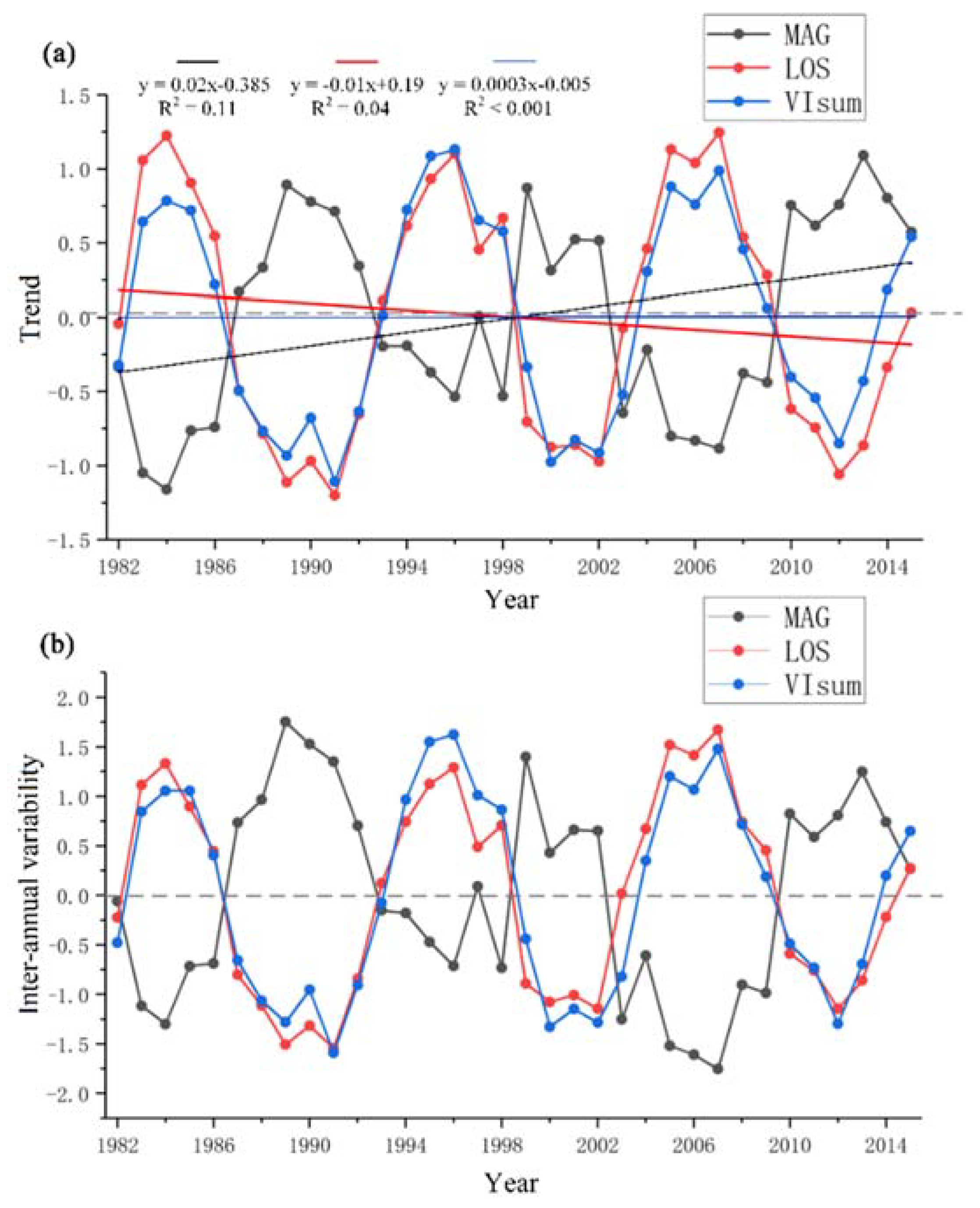
During the past thirty-four years, the overall vegetation productivity (or vegetation greenness) in NEC did not show a significant trend. LOS slightly shortened during the past three decades (declining trend), while MAG presented a relatively strong increasing trend (Figure 3). The inter-annual variability in detrended VIsum, LOS and MAG (Figure 3b) was generally in agreement with the trend in the time series (Figure 3a). There was a potential periodicity in the variability of LOS, MAG and VIsum of approximately ten years (such as in the time range 1985–1995). To accurately quantify the period of the cycle, we determined the dominant frequency of VIsum, LOS, and MAG from a spectral analysis of the time series using the R package ‘forefast’ [43]. This procedure revealed that the dominant frequencies of LOS and VIsum were eleven and ten years, respectively. MAG had a relatively large inter-annual fluctuation and did not exhibit a remarkable period, but visually a shorter period of around 8–12 years could be discerned (but not identified by spectral analysis). The directions of the amplitudes in LOS (VIsum) and MAG showed an opposite pattern, in other words, MAG decreased with increasing LOS. Generally, LOS kept a consistent phase with the changes in VIsum.
Further, in different vegetation types, there were significant differences in spatially-averaged trends for the three variables. The increasing rate of MAG and VIsum in croplands was the highest, with a Sen slope of 0.17 and 0.11, while LOS significantly decreased (Sen slope = −0.15). MAG, LOS and VIsum in needleleaf forests and grasslands tended to increase over time (the forest Sen slope was 0.15, 0.28, 0.09, and grasslands Sen slope was 0.15, 0.06, 0.10). The multi-year averaged MAG, LOS and VIsum in the eastern broad-leaved forests were higher than in other vegetation types, but the rising rate of MAG and VIsum were small (Sen slope was 0.11 and 0.06), while LOS presented a decreasing tendency (Sen slope = −0.08).
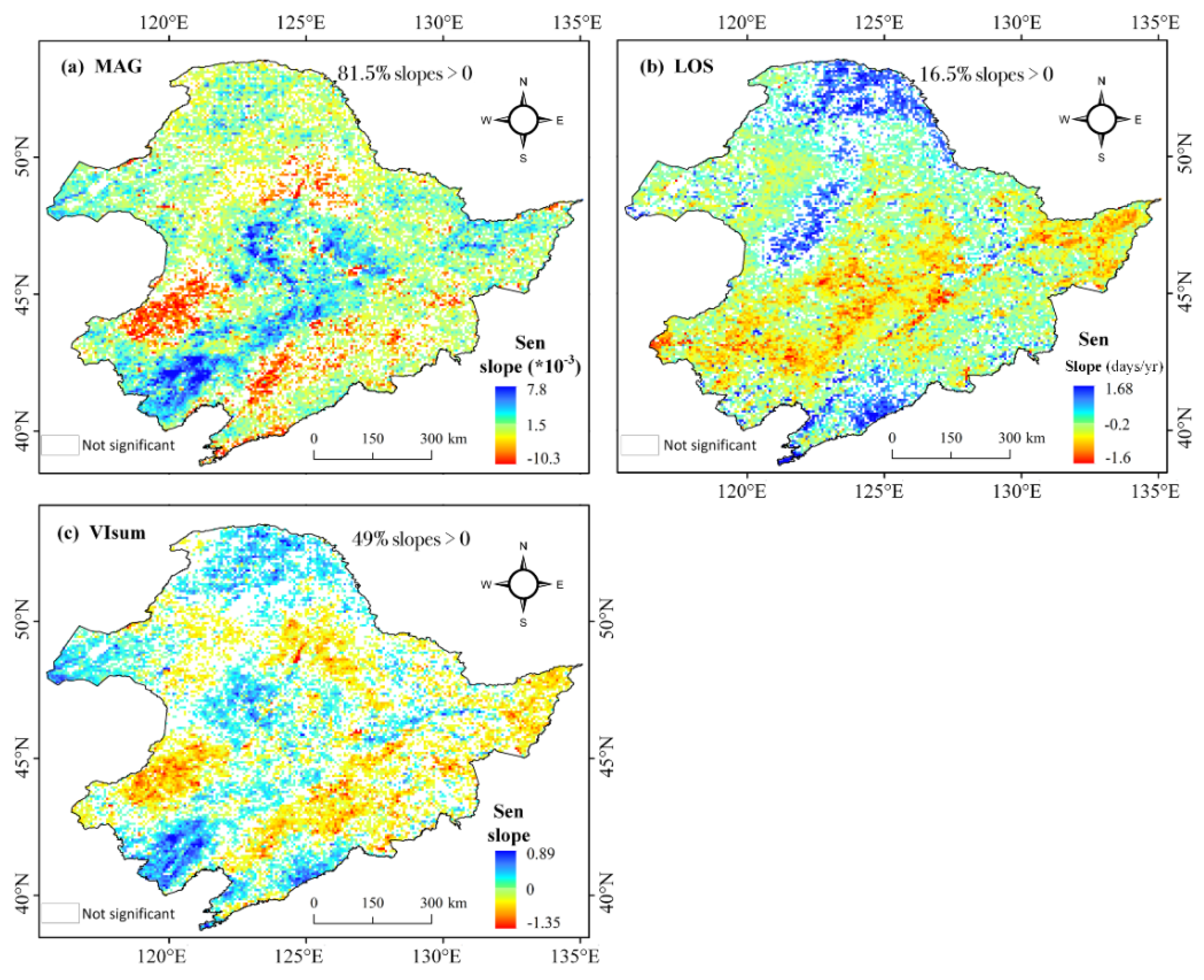
At pixel level, the long-term trends for MAG, LOS, and VIsum were estimated using Theil-Sen slope. The spatial distribution of these trends showed a widespread diversity in different vegetation areas (Figure 4). MAG exhibited a significant positive trend in the central cropland area as well as a weak positive tendency in the northern and eastern forests (about 81.5% of the vegetated areas showed positive trends). However, in the southwestern grassland and the southeastern forest, MAG had a negative trend. LOS with positive trends was mainly distributed in the northern coniferous forest on Daxing’anling Mountains and in a small patch of broad-leaved forest in the southern portion (around 16.5% of the vegetated area showed positive trends). A vast cluster of croplands in the central part showed a negative trend in LOS. There were fewer significant areas of change in summer productivity VIsum than of MAG and LOS. VIsum with positive trends were mainly distributed in the central and southern croplands (about 49% of the vegetated area showed positive trends). VIsum in southwestern grasslands (around 45°N) and eastern forests had a decreasing tendency. In comparison, the spatial segmentation of long-term trends in MAG and VIsum presented a consistent pattern as both of them exhibited positive trends in the central croplands, and negative trends in southwestern grassland and eastern forest. This phenomenon may imply that vegetation growth amplitude plays an essential role in positively affecting vegetation production.
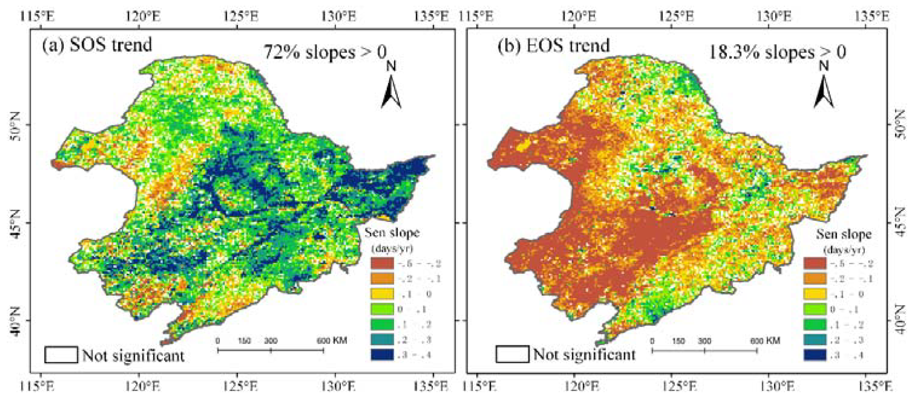
During the past three decades, the Theil-Sen trend of SOS and EOS over the entire NEC was 0.122 days/yr and −0.137 days/yr, respectively, indicating that spring onset was delayed and autumn senescence came earlier. At pixel scale, SOS trends were dominated by positive trends (72% pixels), prominently emerging in central and eastern cultivated vegetation and eastern forest areas (Figure 5a). On the other hand, negative SOS was discretely distributed in the Daxing’anling coniferous forest area, western grassland and a small patch in the southern forest area. In contrast, the majority of EOS had negative trends distributed in central croplands and western grasslands. Positive areas only accounted for 18.3% of the total EOS trends, which significantly occurred in the Daxing’anling coniferous forests, central meadows and in a small patch in the southern forests. The SOS and EOS delayed (positive trend) regions accounted for 72% and 18.3% of the vegetated area, respectively. Overall, the green-up dates for NEC vegetation has been delayed, and the EOS period has arrived earlier.
3.2. Relative Contribution of SOS and EOS to Vegetation Productivity
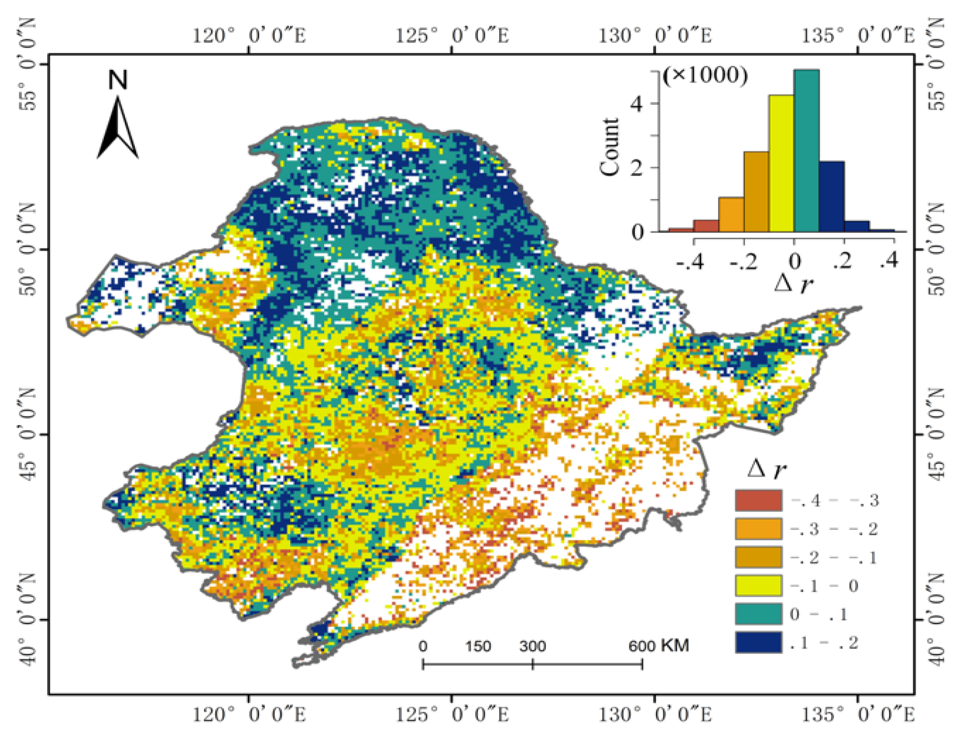
As mentioned above, SOS and EOS play a key role in controlling the seasonal growth cycle of vegetation, and therefore it is important to investigate their impacts on growing season productivity. First, the temporal correlation of SOS and EOS with VIsum over the thirty-four years study period is determined using the Spearman correlation coefficient at pixel scale. Then the spatial characteristics of these correlation coefficients are represented with two raster layers. To compare the magnitude of the relationships between SOS and EOS with VIsum, the absolute values of the two correlation coefficient layers are subtracted (|r_EOS| minus |r_SOS|) to derive the spatial distribution of the differences in the contribution of SOS and EOS to vegetation productivity (Figure 6). According to the sign of the subtraction, vegetation productivity of the northern coniferous forest is more correlated with EOS (positive values), while a vast portion of croplands in NEC have a significant link with SOS (negative values). There are no significant differences between the impacts of SOS and EOS on vegetation productivity in the eastern broad-leaved forest and in the coniferous and broad-leaved mixed forest. In parts of the steppe grassland in the East, SOS is pronouncedly correlated to vegetation productivity. The differences in the effects of the phenological indicators on productivity over different vegetation types can be explained by plant physiological processes and by the trends in the phenological indicators. Herbaceous crops are usually characterized by slow growth and rapid physiological maturity due to their genetic type and artificial management [44], thus EOS of crops will occur earlier than that of natural vegetation. In addition, EOS of crops in this study area shows a negative trend (i.e., it is advanced), so these factors may result in the weak relationship between EOS and vegetation productivity (negative delta values). In contrast, the EOS in the forests of the study area has a delayed trend, so its controlling effect on vegetation productivity is relatively significant.
3.3. Spatial Characteristics of Relative Importance of MAG and LOS to Vegetation Productivity
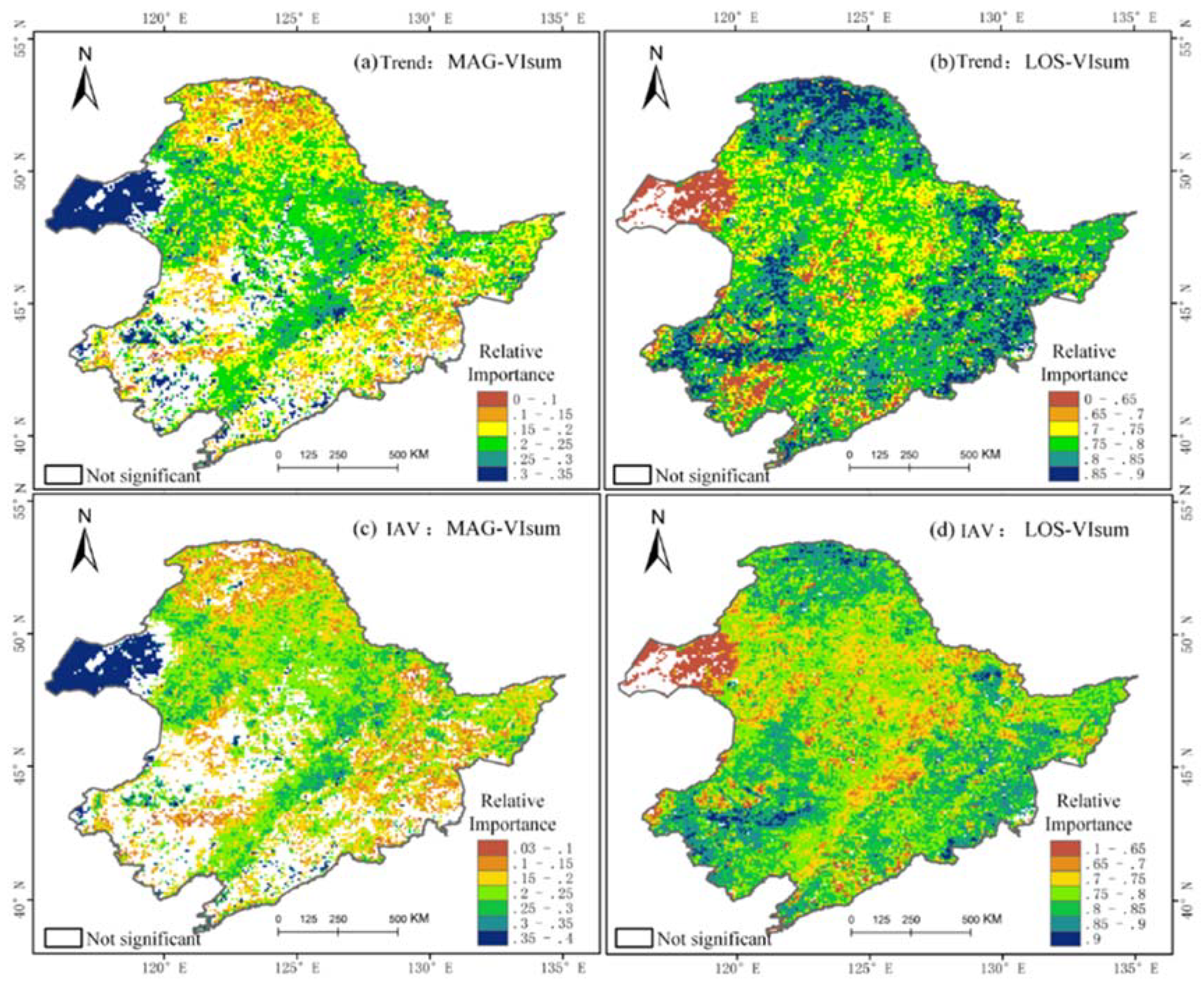
In this paper, the relative importance (RI) approach was used to detect the contribution of MAG and LOS to vegetation production. From the spatial pattern of RI, we found that LOS played a more dominant role than MAG in regulating either the long-term trends (Figure 7a,b) or the inter-annual variability (Figure 7c,d) of vegetation productivity, indicating that summer productivity in each vegetation type was still mainly controlled by LOS, not by MAG. The high RI of MAG was found in the western steppe grassland, followed by central croplands with a relatively smaller RI. Daxing’anling coniferous forests and eastern broad-leaved forests had the lowest RI for MAG. The RI of MAG in the steppe in the southwestern part is not significant. In contrast, the RI of LOS was relatively lower in the western steppe area, but very conspicuous in the Daxing’anling coniferous forests and in the eastern broad-leaved forests. Parts of croplands were slightly controlled by LOS. A visual comparison of Figure 7a,b (row one) with Figure 7c,d (row 2), suggests that the RI of LOS and MAG was likely stronger for long-terms trends than for inter-annual variability across the various vegetation types.
For each vegetation type, Figure 8 shows that LOS was still the main factor controlling the long-term trend of vegetation productivity (mean magnitude of RI around 75%). LOS in the needle- and broad-leaved mixed forest (MF) had the largest contribution to VIsum trends. The relative contribution ratio of MAG to VIsum in each vegetation area was approximately 23%. Although LOS in the steppe area still mainly controlled the long-term trend of productivity, the influencing degree of MAG was significantly greater than that of other vegetation types, which is consistent with the spatial distribution (Figure 7).
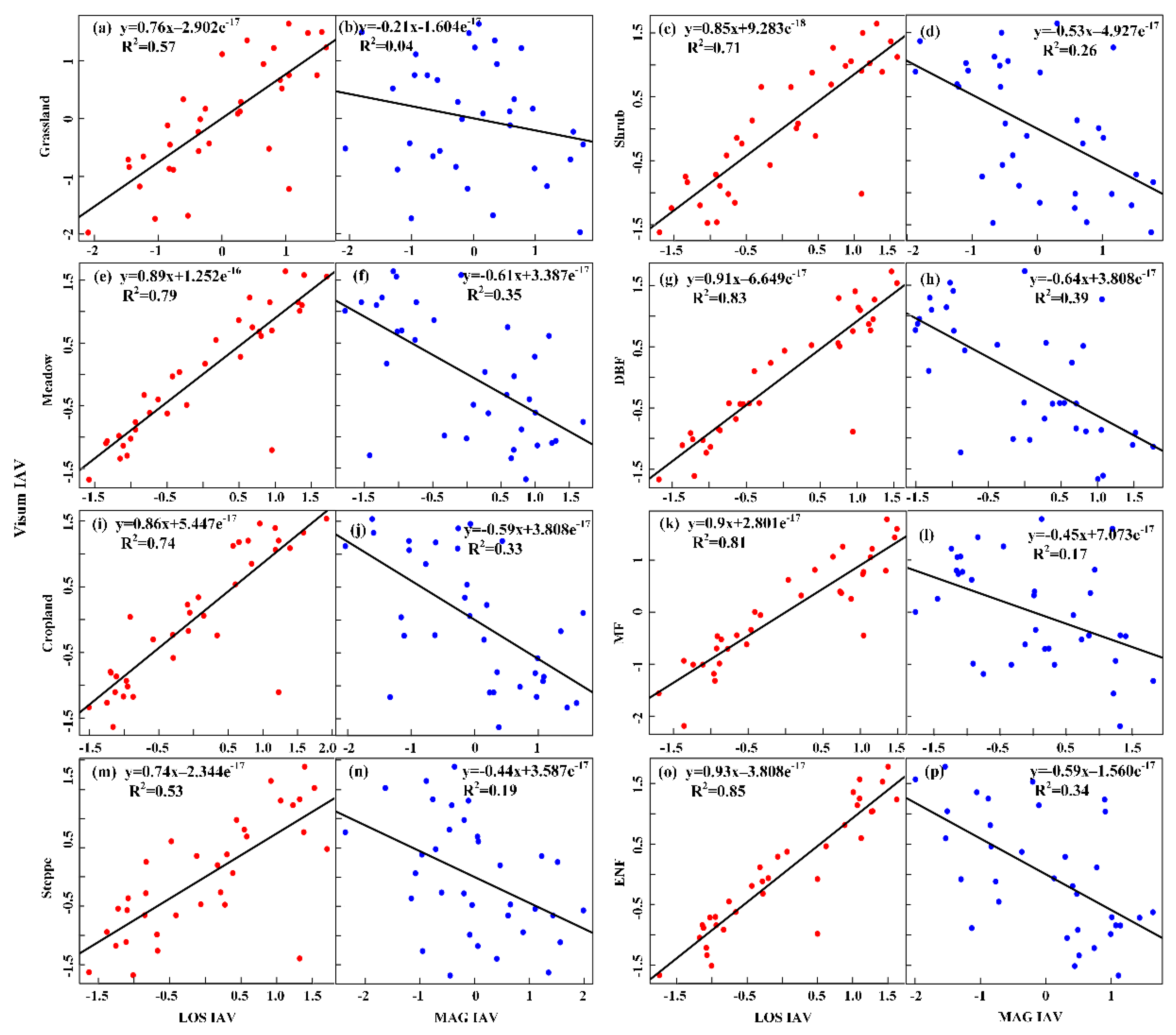
In addition to the long-term trends, we also calculated the IAV of LOS, MAG and VIsum for different vegetation types. The effects of IAV of LOS and MAG on IAV of regional plant productivity (VIsum) were also examined (Figure 9). IAV of VIsum in each region had a significant positive correlation with IAV of LOS, but had an insignificant negative correlation with MAG. In Figure 9, except for grasslands, all other linear regressions were statistically significant (p < 0.01). Among them, the IAV of LOS in the evergreen needleleaf forest (ENF) had the greatest impact on IAV of VIsum (R2 = 0.85), followed in order by needle-leaved, broad-leaved mixed forests (MF) and deciduous broad-leaved forests (DBF). The smallest contribution of IAV of LOS occurred in the steppe area (53%) (Figure 9m). The IAV correlation between MAG and VIsum was most pronounced in DBF forest (R2 = 0.39), followed by meadows, ENF and croplands. IAV of VIsum in grass exhibited the weakest relationship with IAV of MAG. Vegetation growth in croplands is generally intensively regulated by anthropogenic activities (e.g., irrigation, fertilization), and LOS had a greater impact on the variability of productivity (33%). Correlation analysis indicated that the variability of LOS was still the main factor controlling the inter-annual variability of productivity. The impacts of LOS and MAG in forests on productivity variability were the most significant, and the control on productivity variability was the weakest in grassland areas.
4. Discussion
4.1. Plant Phenological Changes over NEC
In the Northern Hemisphere, the impacts of warming-related shifts in seasonality on ecosystem productivity have been extensively investigated [2,16]. Generally, vegetation growing season has progressively lengthened due to both earlier spring and delayed autumn [8] and consequently the photosynthesis period for land vegetation has increased, leading to an increase in vegetation productivity. At the same time, widespread browning and reversal of or stalled greening have been reported at high latitudes [45,46,47]. However, the adaptation of vegetation to climate change in different regions is distinct and limited, so vegetation phenology is location-specific and shows diverse patterns across various biomes. This study identified prominently delayed spring onset over 73% of the vegetated areas and advanced autumn senescence across 82% of the vegetated areas of NEC, which is the opposite of what has been found by some previous studies of the middle and high latitudes of the Northern Hemisphere [14]. The delayed arrival of SOS and the earlier autumn senescence jointly control the shortening of the overall vegetation growing season over NEC. Recent studies have also suggested that the inherently short spring greenup period of northern vegetation will limit its ability to advance further [48,49]. On the other hand, the warming-induced drought stress in autumn will adversely affect the persistence of a delayed end of the growing season [48,49]. The slowing of the SOS advancement since the early 2000s has been well documented over some regions in the Northern Hemisphere, such as Siberia and the Tibetan Plateau [50,51]. These findings could support our results of delayed spring onset and earlier autumn offset.
For the shortening of the cropland growing season, our finding is consistent with the results of a former NPP-based study focusing on NEC [24]. However, this study reveals that the summer peak growth of cultivated vegetation shows an increasing trend over NEC and this may be directly attributed to human farming activities. In addition, warming and CO2 fertilization also indirectly promote peak growth of crops.
According to relative contribution analysis, LOS and MAG jointly control the IAV of VIsum, but present an opposite effect. It is hard for vegetation to maintain a longer LOS and higher MAG concurrently. Thus, the negative temporal correlation between MAG and VIsum may be attributed to the strong positive control of LOS on VIsum. The ten-year periodicity in LOS, MAG and VIsum variability is an interesting finding in this study, which may be attributed to various climatic and gene type factors. As prior study identified, temperature and precipitation have a consistent step with vegetation growth rhythm [52]. From a planet perspective, this periodicity may be caused by the cosmic power. For example, according to our exploratory analysis, these phenological indicators (1982–2015) have a strong correlation with sunspot activity that has been reported an eleven-year periodicity [53,54,55]. This finding highlights the drivers of plant phenological shifts beyond Earth climate.
4.2. Attributing Regulation of Growing Amplitude and Length on Productivity
Across the entire NEC, the insignificant trend in vegetation productivity may be attributed to both shortened LOS and increasing MAG of vegetation greenness. In other words, the shortened duration of the growing season may partly offset the effects of increased greenness amplitude, resulting in the insignificant trend in total vegetation productivity. From the assessment of the relative contribution over different biomes, the impacts of LOS and MAG on the long-term trend and IAV of vegetation productivity are more significant in forests than in various grasslands (Figure 7 and Figure 9). The underlying mechanism may be the much higher productivity and longer growing season of forests compared to grasslands and croplands. However, the contributions of increasing MAG to productivity in croplands and grasslands (mainly steppe) are relatively more pronounced than in forests (Figure 8). Although in this study in both forests and grasslands growing season length has a significant advantage over peak magnitude in controlling IAV of vegetation productivity, this may be altered in the future due to climatic changes and vegetation growth ability. Previous studies have also shown that forest ecosystems are major contributors to land surface productivity, but the maximum growing season amplitude of other vegetation types is likely to continue to increase. Photosynthesic capacity of leaves varies greatly among different vegetation functional types. Studies under the warming condition also showed that the relationship between vegetation growth activity and temperature variability was weakened, and the growing season lengthening was also slowdown [22,56]. Therefore, if the MAG continues to increase, the main controlling effect of the MAG on the carbon sequestration capacity of the vegetation may occur in the future. Recent study also demonstrated that the maximum LAI during the peak growing season accounts for one half of the annual mean LAI, suggesting that growing amplitude played a key in the carbon cycle [12].
The effect of growing season amplitude on productivity trends and variability is greater in herbaceous vegetation areas such as crops and grasslands than in woody vegetation areas such as forests. This is not only related to the ecological functioning of vegetation, but also the impact of human management activities. Recent studies have shown that China and India dominate the increase in global leaf area, mainly due to the contribution of cropland areas [57]. The low herbaceous vegetation has a short growth period, which also highlights the effect of summer growing peaks on productivity development.
4.3. Validation from MODIS EVI
MODIS EVI at 500 m spatial resolution was analyzed to validate the trends and interannual variabilities of VIsum, LOS and MAG (Figure 10). For the entire NEC, all three indices demonstrated a positive trend, in which VIsum and MAG had a significant trend slope. In contrast to the monotonic trend of MODIS EVI-based VIsum, NDVI3g-based VIsum exhibited fluctuations in its temporal variability, which first rised during 2001–2006, then declined until 2012, after which it had an increasing trend. The obvious differences in VIsum trends derived from EVI and NDVI may be attributed to their ability in capturing vegetation greenness. NDVI exhibits a well-known saturation effect over dense vegetated biomes. EVI is enhanced over NDVI through de-coupling of the canopy background signal (through the use of the soil line) and a reduction in atmospheric influences (through the use of the blue band). Thus, cumulative NDVI over the growing season may affect its inter-annual variability and long-term trend. MODIS EVI-based LOS tended to be prolonged slightly, but insignificantly. Although NDVI3g-based LOS showed a slightly shorter trend, it was not statistically significant. In other words, neither of these findings can confirm significant trends for the developing dynamics of LOS. The trend for MODIS EVI-based MAG was in agreement with that derived from NDVI3g, which generally showed an increase during 2001–2015, but with fluctuations. Due to the brevity of the MODIS EVI time series, there no periodic cycle was found in these indices.
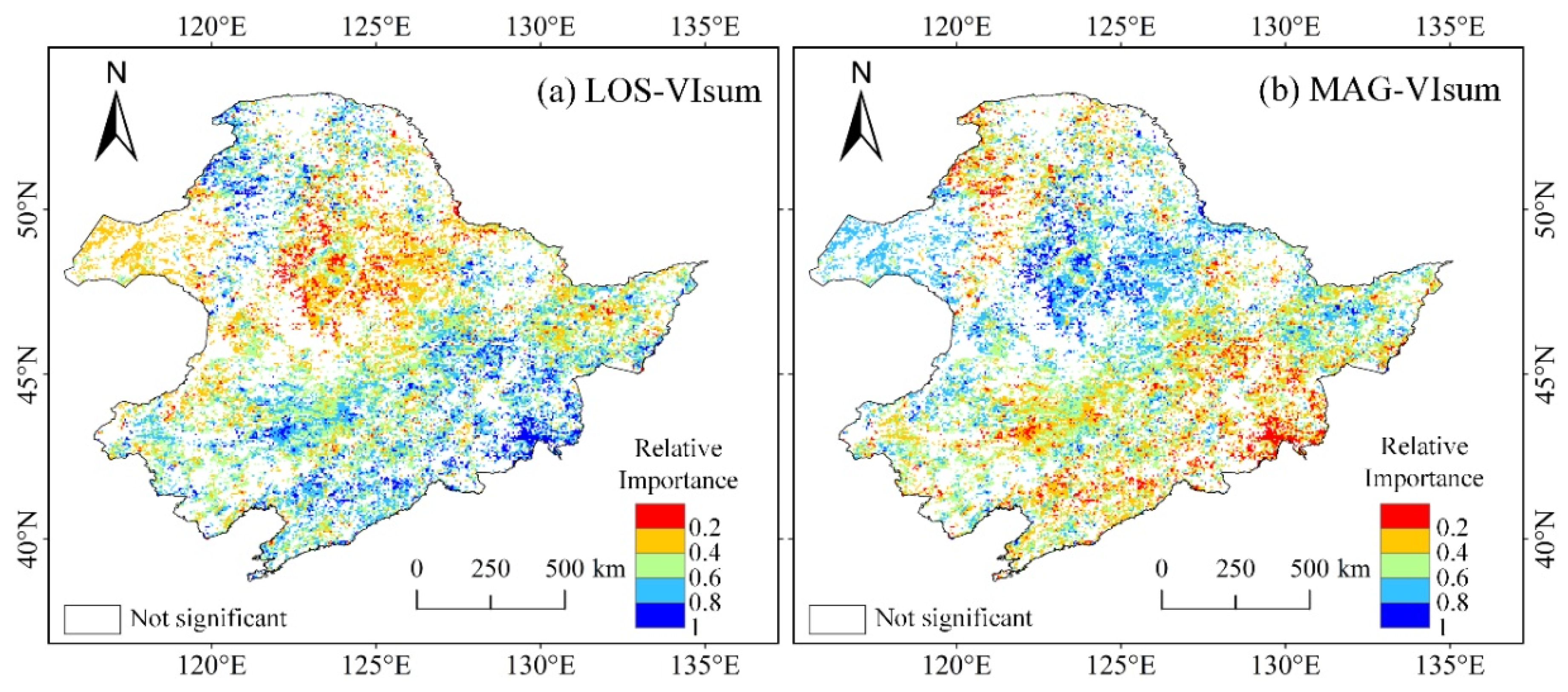
The relative importance of LOS and MAG to VIsum was also examined using the time series dataset of MODIS EVI. Due to the weak impact of IAV, the EVI time series was not decomposed into long-term trend and IAV. Similarly to the NDVI3g derived results (Figure 6), the contributions of LOS and MAG to VIsum exhibited a contrasting spatial pattern (Figure 11). LOS contributed significantly to VIsum in a small extent within the eastern broad-leaved forest and northern coniferous forest, but had a slight impact on VIsum in the central cropland and grassland in the west, whereas MAG played a relatively important role in the eastern grassland and central cropland. It is noteworthy that the contributing magnitude of LOS (mean = 0.51) to VIsum was slightly larger than that of MAG (mean = 0.49). The results that LOS mainly affected forests while MAG was more important in croplands and grasslands were generally in agreement with the results detected with NDVI3g, but with fewer significant pixels.
4.4. Uncertainty Analysis
During the past thirty-four years, anthropogenic activities such as land use and land cover change have also impacted the shift in phenological change patterns due to the conversion of natural vegetated land (forestlands or grassland) into agricultural land over NEC. Further, this phenomenon will create uncertainties in the quantification of the relative contribution of LOS and MAG to growing season productivity. Yet, land cover changes information has to be contained and reflected in the NDVI time series. In other words, the phenological events derived from each NDVI sequence using mature algorithms are generally true and reliable, but they may be the phenological attributions belonging to different vegetation types. To address this issue, we analyzed the land cover changes over NEC. From 1980 to 2000, the shifts in land cover types over NEC were mainly attributed to the conversion of forestlands and grasslands into croplands in DaXing’anling and XiaoXing’anling Mountain areas and of grasslands into croplands in the eastern NEC. During 2000-2006, land cover changes mainly emerged in the Songnen Plain (central part of NEC) with the conversion of dry farmland to paddy farmland and in some degree grasslands to croplands. In general, the more pronounced land cover changes consisted in the conversion of grasslands to croplands and shifts in various agricultural [58]. Due to the 8 km spatial resolution of NDVI and land cover changes occurring mainly in the earlier years of the study period in the NEC, land cover changes probably did not play a dominant role in impacting vegetation phenological dynamics. The long-term trends of SOS and EOS exhibited a similar spatiotemporal pattern in grasslands and croplands that may imply that grasses and crops did not have a significant difference in genetically controlled phenology. Additionally, from Figure 7, we can see that LOS still had the much greater dominant impact factor for vegetation productivity among all vegetation types, so the limited land cover changes would not lead to the reversal of roles LOS and MAG playing in controlling vegetation productivity.
5. Summary and Conclusions
In this paper, the long-term satellite-retrieved vegetation greenness dataset was used to quantify the regulating effects of growing duration length and amplitude on long-term trends and inter-annual variability (IAV) of vegetation productivity over Northeast China (NEC). The conclusions drawn are the following:
- During the past three decades, there was no remarkable change in NDVI-derived vegetation productivity (VIsum) over NEC. However, over vast regions, growing season length (LOS) and amplitude (MAG) presented decreasing and increasing trends, respectively. The temporal profiles for the three phenological variables studied here showed an obvious fluctuation with an approximate cycle of ten years. In the case of persistent trends in LOS and MAG, the regulating effect of MAG on vegetation productivity may be enhanced or even reversed as the main driving force in the future.
- Compared to MAG, LOS was the main factor in controlling the long-term trends and variability of vegetation productivity (VIsum) in NEC. There was a clear spatial cluster characteristic of LOS and MAG in influencing VIsum. The impacts of LOS on VIsum was significant in the northern needleleaf forest and eastern broad-leaved forest, but relatively weak in croplands and steppes. The controlling magnitude of MAG on VIsum was generally small over the whole NEC, with a relatively more pronounced contribution on VIsum in the central-southern croplands and in the western steppe grasslands than in forested areas.
- The key vegetation phenological parameters SOS and EOS indicated a significant shift profile over time. Spatially, SOS was delayed in the majority of NEC (about 72% of vegetated area), except in the northern coniferous forest, and EOS was advanced in the central croplands and western steppe grasslands (about 82% of vegetated area). According to the temporal correlation analysis, EOS had a greater impact on vegetation productivity than SOS in coniferous forest area, while SOS played a more pivotal role than EOS in croplands and in some broadleaf forests.
Overall, this study reveals the spatiotemporal shifts in growing season length and maximum amplitude and their contribution to long-term trends and IAV of vegetation productivity. The approach used here could be utilized in various datasets, such as ground carbon flux and near-ground remote sensing data. Although this is a case study over a temperate zone, it provides broad insights for understanding the mechanisms underlying the trend and IAV of land carbon uptake.
Funding
This work is supported by National Key Research and Development Program (Grant No. 2016YFC0500103, 2018YFB0505301) and National Natural Science Foundation of China (Grant No. 41601478, 41771380). The APC is partly funded by the Key Special Project for Introduced Talents Team of Southern Marine Science and Engineering Guangdong Laboratory (Guangzhou), No. GML2019ZD0301.
Conflicts of Interest
The authors declare no conflict of interest.
Appendix A
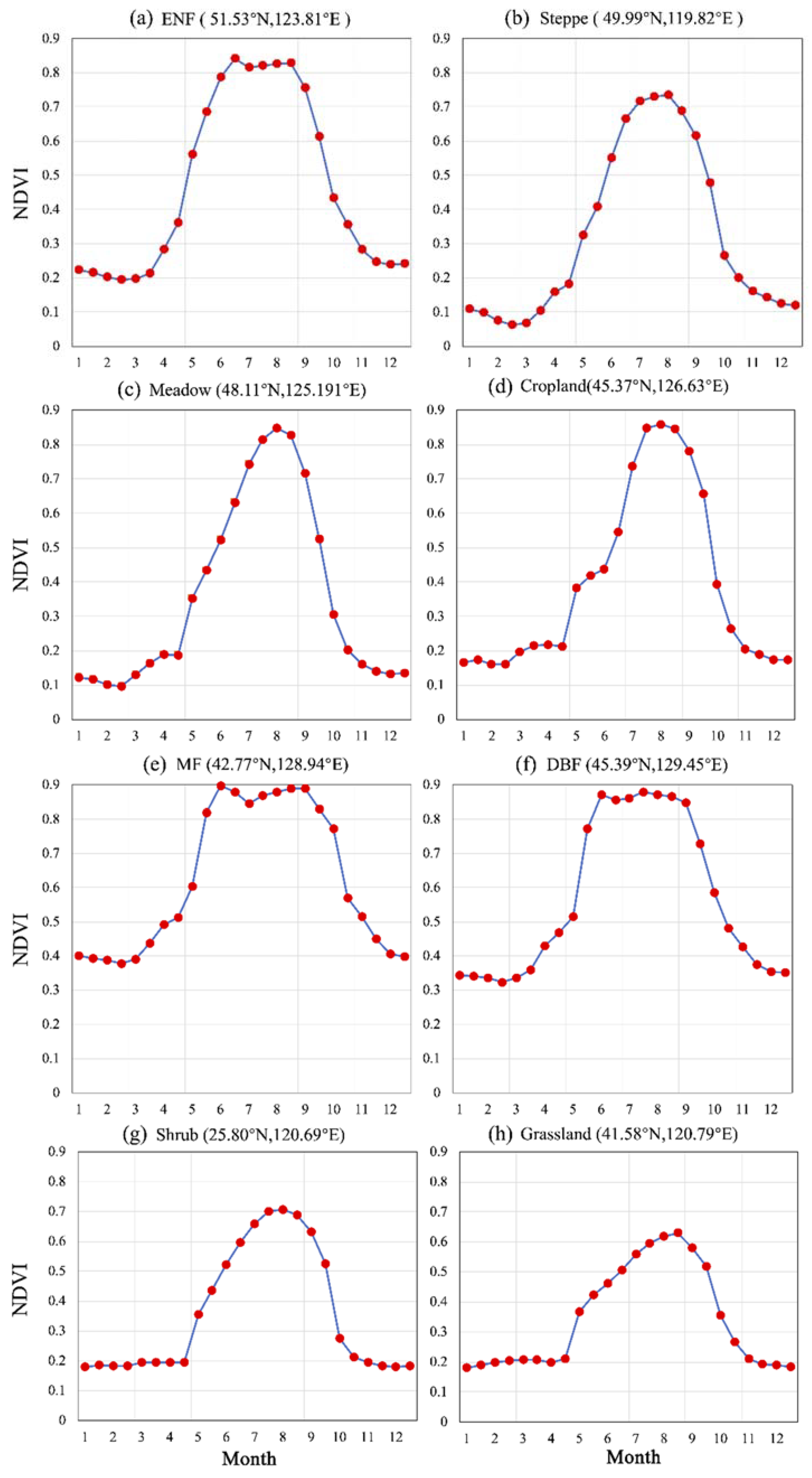
To better understand distinct growth feature of different plants, seasonal growth trajectories for various vegetation types over NEC were depicted in Figure A1. Detailed difference in vegetation growth characteristics could be identified through visually observation. Here, woody plants, such as broad-leaved forest and coniferous forest, generally present a high growth amplitude (high PEAK value) and a long peak growth stage during summer (Figure A1a,e,f). While herbaceous plants have a low PEAK and a sharp growth curve during growing season (Figure A1b–d,g,h).
Figure A1.
Seasonal growth process for typical vegetation covers in NEC (red point denotes multi-year averaged NDVI for a specific time point).
Figure A1.
Seasonal growth process for typical vegetation covers in NEC (red point denotes multi-year averaged NDVI for a specific time point).

References
- Piao, S.; Friedlingstein, P.; Ciais, P.; Zhou, L.; Chen, A. Effect of climate and CO2 changes on the greening of the Northern Hemisphere over the past two decades. Geophys. Res. Lett. 2006, 33, L23402. [Google Scholar] [CrossRef] [Green Version]
- Fu, Z.; Stoy, P.C.; Poulter, B.; Gerken, T.; Zhang, Z.; Wakbulcho, G.; Niu, S. Maximum carbon uptake rate dominates the interannual variability of global net ecosystem exchange. Glob. Chang. Biol. 2019, 25. [Google Scholar] [CrossRef] [Green Version]
- Yang, J.; Dong, J.; Xiao, X.; Dai, J.; Wu, C.; Xia, J.; Zhao, G.; Zhao, M.; Li, Z.; Zhang, Y.; et al. Divergent shifts in peak photosynthesis timing of temperate and alpine grasslands in China. Remote Sens. Environ. 2019, 233, 111395. [Google Scholar] [CrossRef]
- Poulter, B.; Frank, D.; Ciais, P.; Myneni, R.B.; Andela, N.; Bi, J.; Broquet, G.; Canadell, J.G.; Chevallier, F.; Liu, Y.Y.; et al. Contribution of semi-arid ecosystems to interannual variability of the global carbon cycle. Nature 2014, 509, 600–603. [Google Scholar] [CrossRef] [Green Version]
- Piao, S.; Friedlingstein, P.; Ciais, P.; Viovy, N.; Demarty, J. Growing season extension and its impact on terrestrial carbon cycle in the Northern Hemisphere over the past 2 decades. Glob. Biogeochem. Cycles 2007, 21, 1–11. [Google Scholar] [CrossRef]
- Hudson, I.L.; Keatley, M.R. Phenological Research: Methods for Environmental and Climate Change Analysis; Springer: Berlin/Heidelberg, Germany, 2010; ISBN 9048133424. [Google Scholar] [CrossRef]
- Keenan, T.F.; Gray, J.; Friedl, M.A.; Toomey, M.; Bohrer, G.; Hollinger, D.Y.; Munger, J.W.; O’Keefe, J.; Schmid, H.P.; Wing, I.S.; et al. Net carbon uptake has increased through warming-induced changes in temperate forest phenology. Nat. Clim. Chang. 2014, 4, 598–604. [Google Scholar] [CrossRef]
- Richardson, A.D.; Keenan, T.F.; Migliavacca, M.; Ryu, Y.; Sonnentag, O.; Toomey, M. Climate change, phenology, and phenological control of vegetation feedbacks to the climate system. Agric. For. Meteorol. 2013, 169, 156–173. [Google Scholar] [CrossRef]
- Xia, J.; Wan, S. The effects of warming-shifted plant phenology on ecosystem carbon exchange are regulated by precipitation in a semi-arid grassland. PLoS ONE 2012, 7, e32088. [Google Scholar] [CrossRef] [PubMed] [Green Version]
- Myneni, R.B.; Keeling, C.D.; Tucker, C.J.; Asrar, G.; Nemani, R.R. Increased plant growth in the northern high latitudes from 1981 to 1991. Nature 1997, 386, 698–702. [Google Scholar] [CrossRef]
- Richardson, A.D.; Andy Black, T.; Ciais, P.; Delbart, N.; Friedl, M.A.; Gobron, N.; Hollinger, D.Y.; Kutsch, W.L.; Longdoz, B.; Luyssaert, S.; et al. Influence of spring and autumn phenological transitions on forest ecosystem productivity. Philos. Trans. R. Soc. B Biol. Sci. 2010, 365, 3227–3246. [Google Scholar] [CrossRef] [PubMed] [Green Version]
- Chen, J.M.; Ju, W.; Ciais, P.; Viovy, N.; Liu, R.; Liu, Y.; Lu, X. Vegetation structural change since 1981 significantly enhanced the terrestrial carbon sink. Nat. Commun. 2019, 10, 4259. [Google Scholar] [CrossRef] [PubMed]
- Huang, K.; Xia, J.; Wang, Y.; Ahlström, A.; Chen, J.; Cook, R.B.; Cui, E.; Fang, Y.; Fisher, J.B.; Huntzinger, D.N. Enhanced peak growth of global vegetation and its key mechanisms. Nat. Ecol. Evol. 2018, 2, 1897–1905. [Google Scholar] [CrossRef] [PubMed]
- Reyes-Fox, M.; Steltzer, H.; Trlica, M.J.; McMaster, G.S.; Andales, A.A.; LeCain, D.R.; Morgan, J.A. Elevated CO2 further lengthens growing season under warming conditions. Nature 2014, 510, 259–262. [Google Scholar] [CrossRef] [PubMed]
- Buermann, W.; Bikash, P.R.; Jung, M.; Burn, D.H.; Reichstein, M. Earlier springs decrease peak summer productivity in North American boreal forests. Environ. Res. Lett. 2013, 8, 024027. [Google Scholar] [CrossRef]
- Buermann, W.; Forkel, M.; O’Sullivan, M.; Sitch, S.; Friedlingstein, P.; Haverd, V.; Jain, A.K.; Kato, E.; Kautz, M.; Lienert, S.; et al. Widespread seasonal compensation effects of spring warming on northern plant productivity. Nature 2018, 562, 110–114. [Google Scholar] [CrossRef] [Green Version]
- Zhu, W.; Pan, Y.; Liu, X.; Wang, A. Spatio-temporal distribution of net primary productivity along the Northeast China Transect and its response to climatic change. J. For. Res. 2006, 17, 93–98. [Google Scholar] [CrossRef]
- Ni, J.; Wang, G.-H. Northeast China Transect (NECT): Ten-year synthesis and future challenges. ACTA Bot. Sin. Engl. Ed. 2004, 46, 379–391. [Google Scholar]
- Zhang, X.S.; Gao, Q.; Yang, D.A.; Zhou, G.S.; Ni, J.; Wang, Q. A gradient analysis and prediction on the Northeast China Transect (NECT) for global change study. Acta Bot. Sin. 1997, 39, 785–799. [Google Scholar]
- Yu, L.; Liu, T.; Bu, K.; Yan, F.; Yang, J.; Chang, L.; Zhang, S. Monitoring the long term vegetation phenology change in Northeast China from 1982 to 2015. Sci. Rep. 2017, 7, 14770. [Google Scholar] [CrossRef] [Green Version]
- Yu, X.; Zhuang, D. Monitoring forest phenophases of Northeast China based on MODIS NDVI data. Resour. Sci. 2006, 28, 111–117. [Google Scholar]
- Piao, S.; Fang, J.; Zhou, L.; Ciais, P.; Zhu, B. Variations in satellite-derived phenology in China’s temperate vegetation. Glob. Chang. Biol. 2006, 12, 672–685. [Google Scholar] [CrossRef]
- Chen, X.; Hu, B.; Yu, R. Spatial and temporal variation of phenological growing season and climate change impacts in temperate eastern China. Glob. Chang. Biol. 2005, 11, 1118–1130. [Google Scholar] [CrossRef]
- Qiu, Y.; Fan, D.; Zhao, X.; Sun, W. Spatio-temporal Changes of NPP and Its Responses to Phenology in Northeast China. Geogr. Geo-Inf. Sci. 2017, 33, 21–27. [Google Scholar] [CrossRef]
- Ni, J.; Zhang, X.S. Climate variability ecological gradient and the Northeast China Transect (NECT). J. Arid Environ. 2000, 46, 313–325. [Google Scholar] [CrossRef] [Green Version]
- Editorial Committee for Vegetation Map of China. Vegetation Map of the People’s Republic of China (1:1 000 000); Geological Publishing House: Beijing, China, 2007. [Google Scholar]
- Pettorelli, N.; Vik, J.O.; Mysterud, A.; Gaillard, J.M.; Tucker, C.J.; Stenseth, N.C. Using the satellite-derived NDVI to assess ecological responses to environmental change. Trends Ecol. Evol. 2005, 20, 503–510. [Google Scholar] [CrossRef]
- Tucker, C.J.; Pinzon, J.E.; Brown, M.E.; Slayback, D.A.; Pak, E.W.; Mahoney, R.; Vermote, E.F.; El Saleous, N. An extended AVHRR 8-km NDVI dataset compatible with MODIS and SPOT vegetation NDVI data. Int. J. Remote Sens. 2005, 26, 4485–4498. [Google Scholar] [CrossRef]
- Gitelson, A.A.; Peng, Y.; Masek, J.G.; Rundquist, D.C.; Verma, S.; Suyker, A.; Baker, J.M.; Hatfield, J.L.; Meyers, T. Remote estimation of crop gross primary production with Landsat data. Remote Sens. Environ. 2012, 121, 404–414. [Google Scholar] [CrossRef] [Green Version]
- Running, S.W.; Thornton, P.E.; Nemani, R.; Glassy, J.M. Global Terrestrial Gross and Net Primary Productivity from the Earth Observing System. In Methods in Ecosystem Science; Springer: New York, NY, USA, 2000; pp. 44–57. [Google Scholar] [CrossRef]
- Gichenje, H.; Godinho, S. Establishing a land degradation neutrality national baseline through trend analysis of GIMMS NDVI Time-series. Land Degrad. Dev. 2018, 29, 2985–2997. [Google Scholar] [CrossRef]
- Chu, H.; Venevsky, S.; Wu, C.; Wang, M. NDVI-based vegetation dynamics and its response to climate changes at Amur-Heilongjiang River Basin from 1982 to 2015. Sci. Total Environ. 2019, 650, 2051–2062. [Google Scholar] [CrossRef]
- Fan, X.; Liu, Y. Multisensor Normalized Difference Vegetation Index Intercalibration: A Comprehensive Overview of the Causes of and Solutions for Multisensor Differences. IEEE Geosci. Remote Sens. Mag. 2018, 6, 23–45. [Google Scholar] [CrossRef]
- Pinzon, J.E.; Tucker, C.J. A non-stationary 1981–2012 AVHRR NDVI3g time series. Remote Sens. 2014, 6, 6929–6960. [Google Scholar] [CrossRef] [Green Version]
- Chen, J.; Jönsson, P.; Tamura, M.; Gu, Z.; Matsushita, B.; Eklundh, L. A simple method for reconstructing a high-quality NDVI time-series data set based on the Savitzky–Golay filter. Remote Sens. Environ. 2004, 91, 332–344. [Google Scholar] [CrossRef]
- Press, W.H.; Teukolsky, S.A. Savitzky-Golay smoothing filters. Comput. Phys. 1990, 4, 669–672. [Google Scholar] [CrossRef]
- Beck, H.E.; McVicar, T.R.; van Dijk, A.I.J.M.; Schellekens, J.; de Jeu, R.A.M.; Bruijnzeel, L.A. Global evaluation of four AVHRR–NDVI data sets: Intercomparison and assessment against Landsat imagery. Remote Sens. Environ. 2011, 115, 2547–2563. [Google Scholar] [CrossRef]
- Reed, B.C.; Brown, J.F.; VanderZee, D.; Loveland, T.R.; Merchant, J.W.; Ohlen, D.O. Measuring phenological variability from satellite imagery. J. Veg. Sci. 1994, 5, 703–714. [Google Scholar] [CrossRef]
- Fu, Z.; Dong, J.; Zhou, Y.; Stoy, P.C.; Niu, S. Long term trend and interannual variability of land carbon uptake—The attribution and processes. Environ. Res. Lett. 2017, 12. [Google Scholar] [CrossRef]
- Grömping, U. Relative importance for linear regression in R: The package relaimpo. J. Stat. Softw. 2006, 17, 1–27. [Google Scholar] [CrossRef] [Green Version]
- Neeti, N.; Eastman, J.R. A contextual mann-kendall approach for the assessment of trend significance in image time series. Trans. GIS 2011, 15, 599–611. [Google Scholar] [CrossRef]
- Sayemuzzaman, M.; Jha, M.K. Seasonal and annual precipitation time series trend analysis in North Carolina, United States. Atmos. Res. 2014, 137, 183–194. [Google Scholar] [CrossRef]
- Hyndman, R.J.; Khandakar, Y. Automatic Time Series Forecasting: The Forecast Package for R; Department of Econometrics and Business Statistics, Monash University: Mebourne, Australia, 2007. [Google Scholar] [CrossRef] [Green Version]
- Garcia del Moral, L.F.; Miralles, D.J.; Slafer, G.A. Initiation and Appearance of Vegetative and Reproductive Structures throughout Barley Development. Barley Sci. Recent Adv. Mol. Biol. Agron. Yield Qual. 2002, 243. [Google Scholar]
- Gonsamo, A.; Ter-Mikaelian, M.T.; Chen, J.M.; Chen, J. Does Earlier and Increased Spring Plant Growth Lead to Reduced Summer Soil Moisture and Plant Growth on Landscapes Typical of Tundra-Taiga Interface? Remote Sens. 2019, 11, 1989. [Google Scholar] [CrossRef] [Green Version]
- Menzel, A.; Sparks, T.H.; Estrella, N.; Koch, E.; Aaasa, A.; Ahas, R.; Alm-Kübler, K.; Bissolli, P.; Braslavská, O.; Briede, A.; et al. European phenological response to climate change matches the warming pattern. Glob. Chang. Biol. 2006, 12, 1969–1976. [Google Scholar] [CrossRef]
- Ibáñez, I.; Primack, R.B.; Miller-Rushing, A.J.; Ellwood, E.; Higuchi, H.; Lee, S.D.; Kobori, H.; Silander, J.A. Forecasting phenology under global warming. Philos. Trans. R. Soc. B Biol. Sci. 2010, 365, 3247–3260. [Google Scholar] [CrossRef] [PubMed]
- Wu, C.; Wang, X.; Wang, H.; Ciais, P.; Peñuelas, J.; Myneni, R.B.; Desai, A.R.; Gough, C.M.; Gonsamo, A.; Black, A.T. Contrasting responses of autumn-leaf senescence to daytime and night-time warming. Nat. Clim. Chang. 2018, 8, 1092. [Google Scholar] [CrossRef] [Green Version]
- Park, H.; Jeong, S.-J.; Ho, C.-H.; Park, C.-E.; Kim, J. Slowdown of spring green-up advancements in boreal forests. Remote Sens. Environ. 2018, 217, 191–202. [Google Scholar] [CrossRef]
- Wang, X.; Piao, S.; Xu, X.; Ciais, P.; Macbean, N.; Myneni, R.B.; Li, L. Has the advancing onset of spring vegetation green-up slowed down or changed abruptly over the last three decades? Glob. Ecol. Biogeogr. 2015, 24, 621–631. [Google Scholar] [CrossRef]
- Wang, X.; Xiao, J.; Li, X.; Cheng, G.; Ma, M.; Zhu, G.; Altaf Arain, M.; Andrew Black, T.; Jassal, R.S. No trends in spring and autumn phenology during the global warming hiatus. Nat. Commun. 2019, 10, 2389. [Google Scholar] [CrossRef]
- Zhou, Y. Asymmetric Behavior of Vegetation Seasonal Growth and the Climatic Cause: Evidence from Long-Term NDVI Dataset in Northeast China. Remote Sens. 2019, 11, 2107. [Google Scholar] [CrossRef] [Green Version]
- Surový, P.; Ribeiro, N.A.; Pereira, J.S.; Dorotovič, I. Influence of solar activity cycles on cork growth—A hypothesis. In Proceedings of the 19th National Solar Physics Meeting, Papradno; Dorotovič, I., Ed.; SÚH: Hurbanovo, Slovakia, 2008; p. 67, published on CD. [Google Scholar]
- Woodborne, S.; Mélice, J.L.; Scholes, R.J. Long-term sunspot forcing of savanna structure inferred from carbon and oxygen isotopes. Geophys. Res. Lett. 2008, 35. [Google Scholar] [CrossRef]
- Harrison, V.L. Do Sunspot Cycles Affect Crop Yields; Agricultural Economic Report No. 327; Economic Research Service, US Department of Agriculture: Washing, DC, USA, 1974.
- Angert, A.; Biraud, S.; Bonfils, C.; Henning, C.C.; Buermann, W.; Pinzon, J.; Tucker, C.J.; Fung, I. Drier summers cancel out the CO2 uptake enhancement induced by warmer springs. Proc. Natl. Acad. Sci. USA 2005, 102, 10823–10827. [Google Scholar] [CrossRef] [Green Version]
- Chen, C.; Park, T.; Wang, X.; Piao, S.; Xu, B.; Chaturvedi, R.K.; Fuchs, R.; Brovkin, V.; Ciais, P.; Fensholt, R.; et al. China and India lead in greening of the world through land-use management. Nat. Sustain. 2019, 2, 122–129. [Google Scholar] [CrossRef] [PubMed]
- Liu, J.; Kuang, W.; Zhang, Z.; Xu, X.; Qin, Y.; Ning, J.; Zhou, W.; Zhang, S.; Li, R.; Yan, C. Spatiotemporal characteristics, patterns, and causes of land-use changes in China since the late 1980s. J. Geogr. Sci. 2014, 24, 195–210. [Google Scholar] [CrossRef]
Figure 1.
Elevation map (a) and vegetation types (b) in Northeast China (NEC)
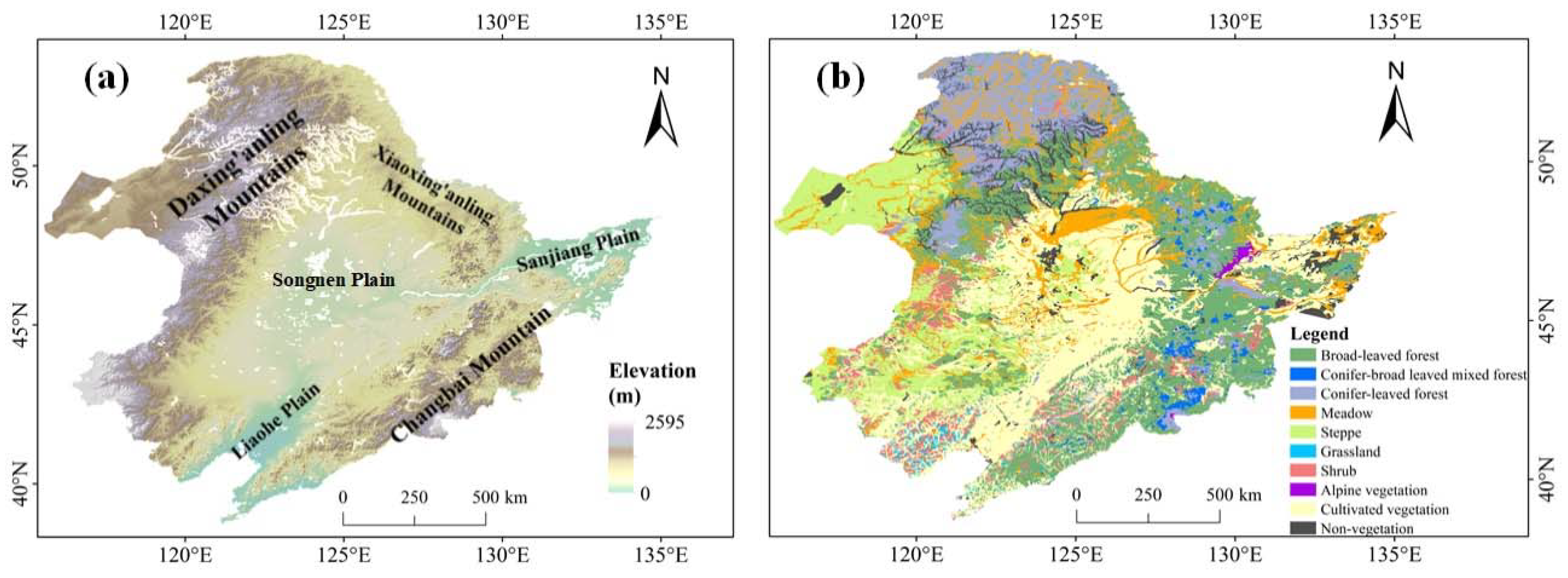
Figure 2.
Schematic diagram depicting the growth curve and key phenological parameters. Circles represent remote sensing normalized difference vegetation index (NDVI), the blue line is fitting growth curve, the oblique orange lines denote tangent lines at SOS, EOS; SOS: Start of growing season, EOS: End of growing season, LOS: Length of growing season, MAG: PEAK minus Baseline Value

Figure 3.
Long-term trends (a) and inter-annual variability (b) of VIsum,LOS, and MAG for the entire Northeast China (straight lines represent linear regression trends).
Figure 3.
Long-term trends (a) and inter-annual variability (b) of VIsum,LOS, and MAG for the entire Northeast China (straight lines represent linear regression trends).

Figure 4.
Spatial distribution of Theil-Sen Trends for MAG (a), LOS (b) and VIsum (c), (LOS units: days/year; MAG and VIsum are unitless, significance level: p value < 0.05)
Figure 4.
Spatial distribution of Theil-Sen Trends for MAG (a), LOS (b) and VIsum (c), (LOS units: days/year; MAG and VIsum are unitless, significance level: p value < 0.05)

Figure 5.
Spatial distribution of long-term trends for SOS and EOS (unit: days/yr, significance level: p value < 0.05). (a) map of SOS trend, (b) map of EOS trend.
Figure 5.
Spatial distribution of long-term trends for SOS and EOS (unit: days/yr, significance level: p value < 0.05). (a) map of SOS trend, (b) map of EOS trend.

Figure 6.
Spatial distribution of the difference in the correlation coefficients for EOS vs. VIsum and SOS vs. VIsum.
Figure 6.
Spatial distribution of the difference in the correlation coefficients for EOS vs. VIsum and SOS vs. VIsum.

Figure 7.
Spatial distribution of relative importance of MAG and LOS to long-term trends (a,b) and inter-annual variability (IAV) (c,d) of vegetation production (significance level: p value < 0.05).
Figure 7.
Spatial distribution of relative importance of MAG and LOS to long-term trends (a,b) and inter-annual variability (IAV) (c,d) of vegetation production (significance level: p value < 0.05).

Figure 8.
Relative importance (RI) of LOS and MAG to trends of vegetation productivity in different vegetation types. Bar height is the mean value for each vegetation type; the error bar denotes one standard deviation. ENF: evergreen needle-leaved forest. DBF: Deciduous broad-leaved forest. MF: mixed forest.
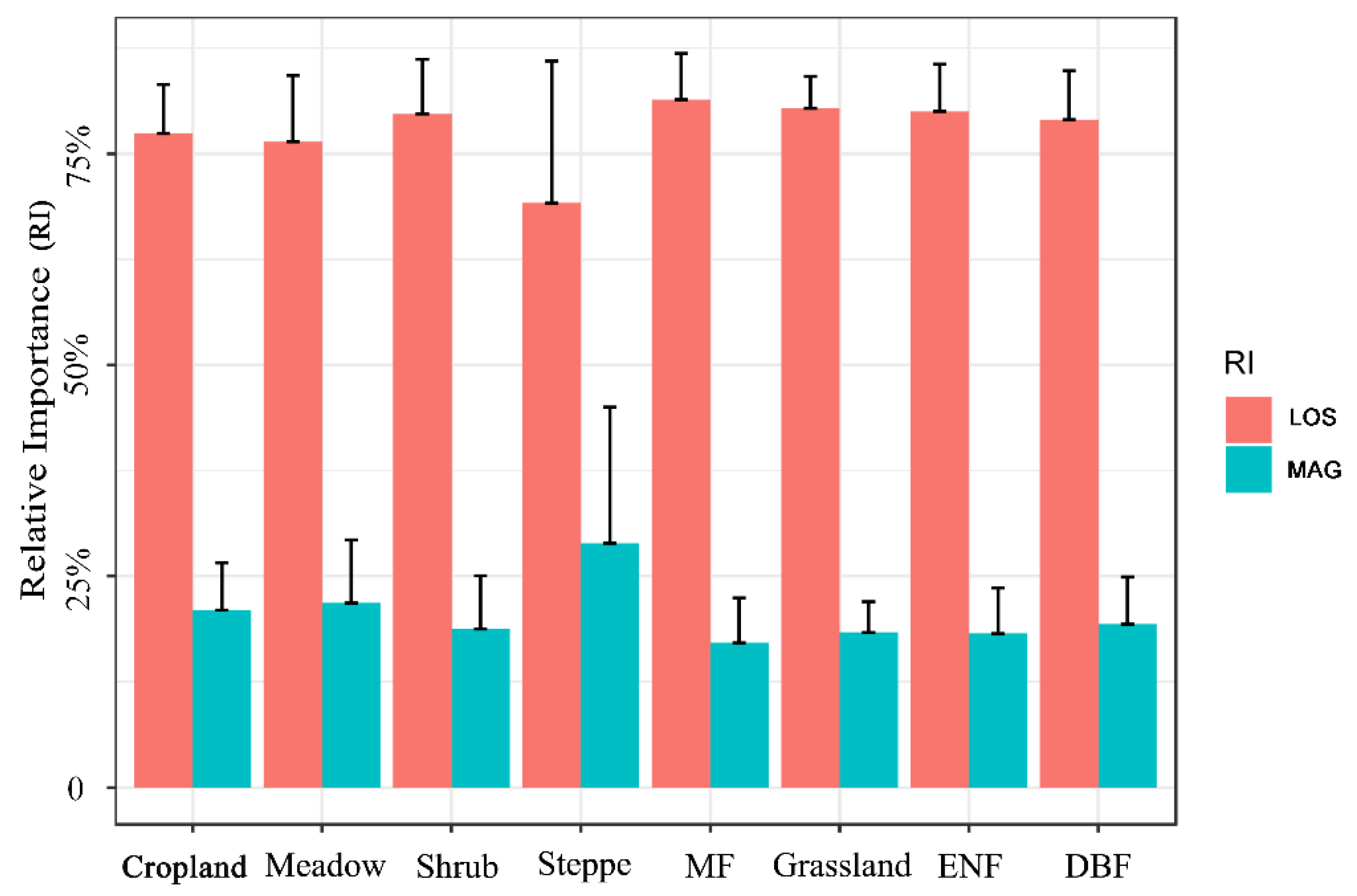
Figure 9.
Correlations of VIsum IAV with IAV in LOS and MAG for different vegetation types (rows represent vegetation types, panels with red points denote LOS IAV, panels with blue points denote MAG IAV). (a,b) is the correlations in grassland; (c,d) in shrubland; (e,f) in meadow; (g,h) in deciduous broad-leaved forest; (i,j) in cropland; (k,l) in needle- and broad-leaved mixed forest; (m,n) in steppe; (o,p) in evergreen needle-leaved forest.

Figure 10.
Temporal variations of VIsum, LOS and MAG (in rows) derived from MODIS EVI (a–c) and NDVI3g (d–f). (a–c) is VIsum, LOS and MAG from MODIS EVI, respectively. (d–f) is VIsum, LOS and MAG from NDVI3g, respectively.
Figure 10.
Temporal variations of VIsum, LOS and MAG (in rows) derived from MODIS EVI (a–c) and NDVI3g (d–f). (a–c) is VIsum, LOS and MAG from MODIS EVI, respectively. (d–f) is VIsum, LOS and MAG from NDVI3g, respectively.
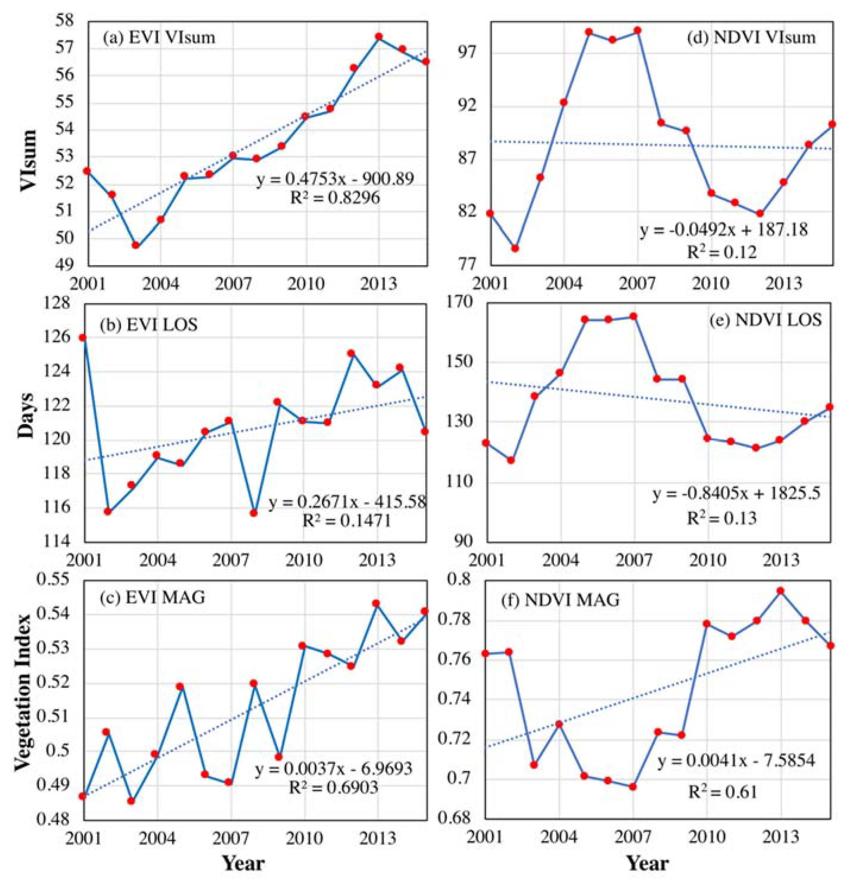
Figure 11.
Maps of the relative importance of LOS (a) and MAG (b) to VIsum derived MODIS EVI

© 2020 by the author. Licensee MDPI, Basel, Switzerland. This article is an open access article distributed under the terms and conditions of the Creative Commons Attribution (CC BY) license (http://creativecommons.org/licenses/by/4.0/).
Share and Cite
MDPI and ACS Style
Zhou, Y. Relative Contribution of Growing Season Length and Amplitude to Long-Term Trend and Interannual Variability of Vegetation Productivity over Northeast China. Forests 2020, 11, 112. https://0-doi-org.brum.beds.ac.uk/10.3390/f11010112
AMA Style
Zhou Y. Relative Contribution of Growing Season Length and Amplitude to Long-Term Trend and Interannual Variability of Vegetation Productivity over Northeast China. Forests. 2020; 11(1):112. https://0-doi-org.brum.beds.ac.uk/10.3390/f11010112
Chicago/Turabian StyleZhou, Yuke. 2020. "Relative Contribution of Growing Season Length and Amplitude to Long-Term Trend and Interannual Variability of Vegetation Productivity over Northeast China" Forests 11, no. 1: 112. https://0-doi-org.brum.beds.ac.uk/10.3390/f11010112
Note that from the first issue of 2016, this journal uses article numbers instead of page numbers. See further details here.