Shallow Landslide Susceptibility Mapping by Random Forest Base Classifier and Its Ensembles in a Semi-Arid Region of Iran

 , ,
, ,  ,
, 
 ,
,  , ,
, , 
Abstract
:1. Introduction
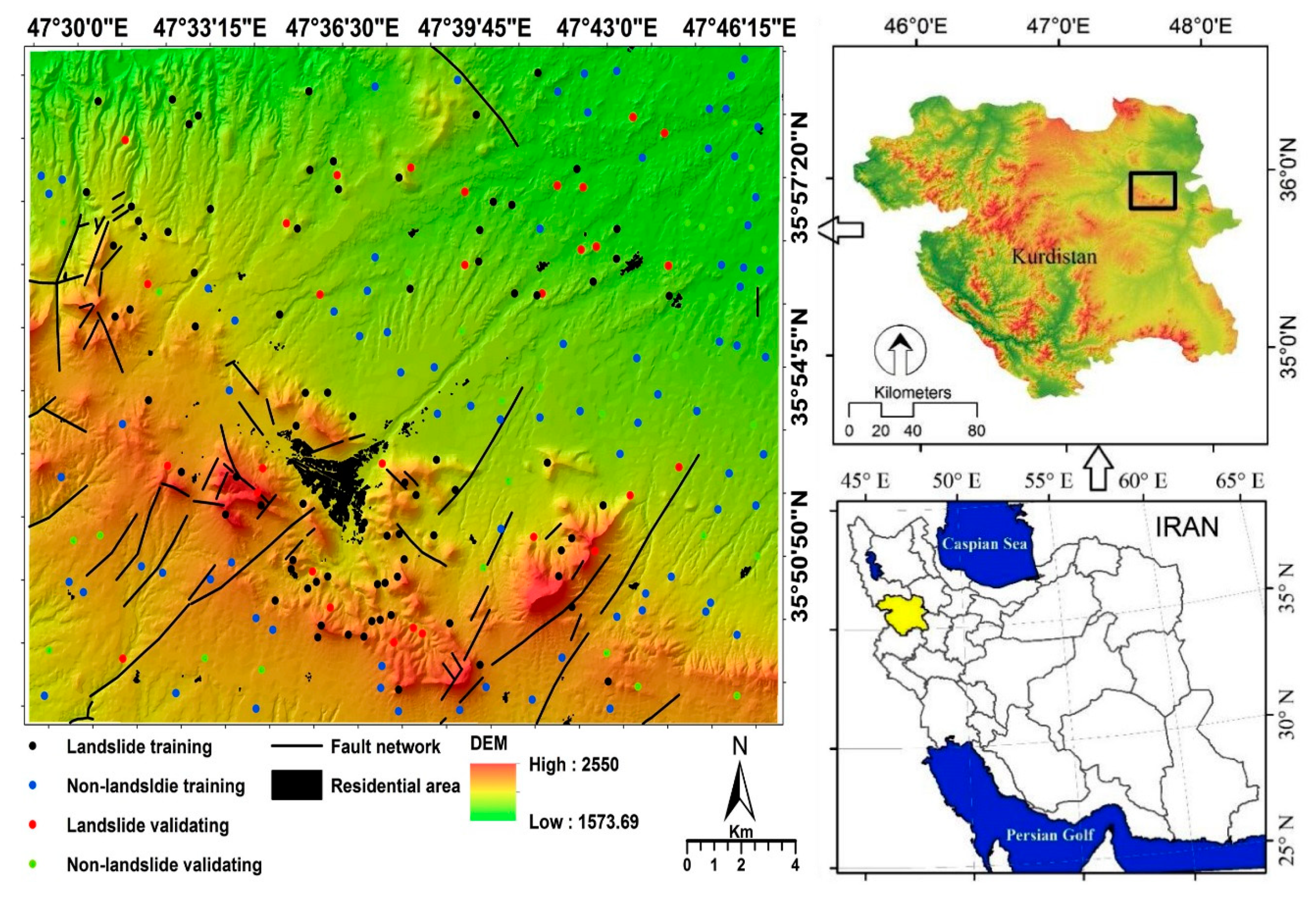
2. Study Area
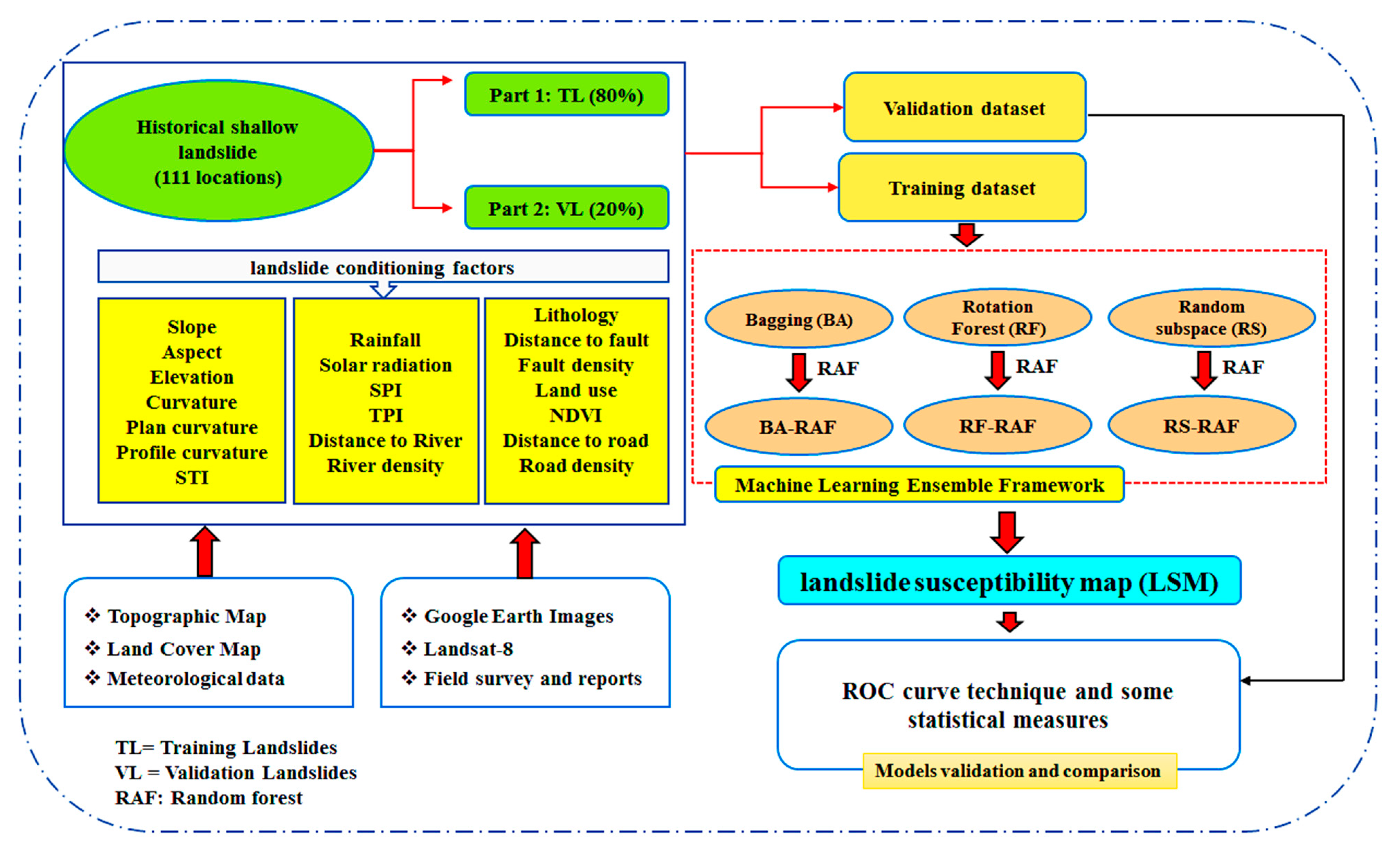
3. Data Preparation
3.1. Landslide Inventory Map
3.2. Landslide Conditioning Factors
4. Machine Learning Models
4.1. Random Forest Decision Tree-Base Classifier
4.2. Ensemble Models
4.2.1. Bagging
4.2.2. Random Subspace
4.2.3. Rotation Forest
4.3. Model Validation and Comparison
4.3.1. Statistical Metrics
- (i)
- One group is used to evaluate the generalization ability of the trained classifier, more specifically the performance of trained classifier when tested with an unseen dataset.
- (ii)
- A second group is employed in evaluating model selection. The aim is to select the optimum classifier among a variety of trained classifiers based on their performance using an unseen dataset.
- (iii)
- A third group selects the optimum solution among all solutions generated during the classification training. Only the optimum solution obtained from the optimum model is tested with the unseen dataset.
4.3.2. ROC and AUC
4.3.3. Friedman and Wilcoxon Sign Rank Tests
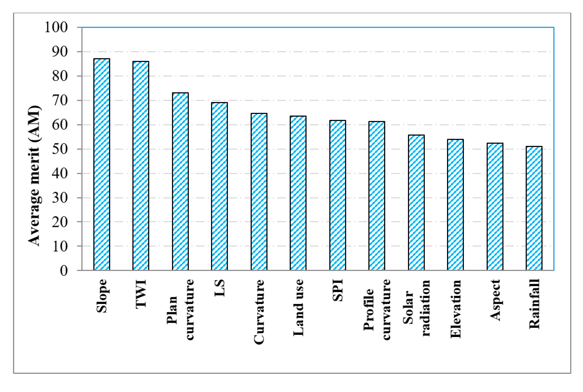
4.4. Factor Selection Using the Information Gain Ratio Technique
5. Analysis and Results
5.1. Factor Selection in Modeling Landslides
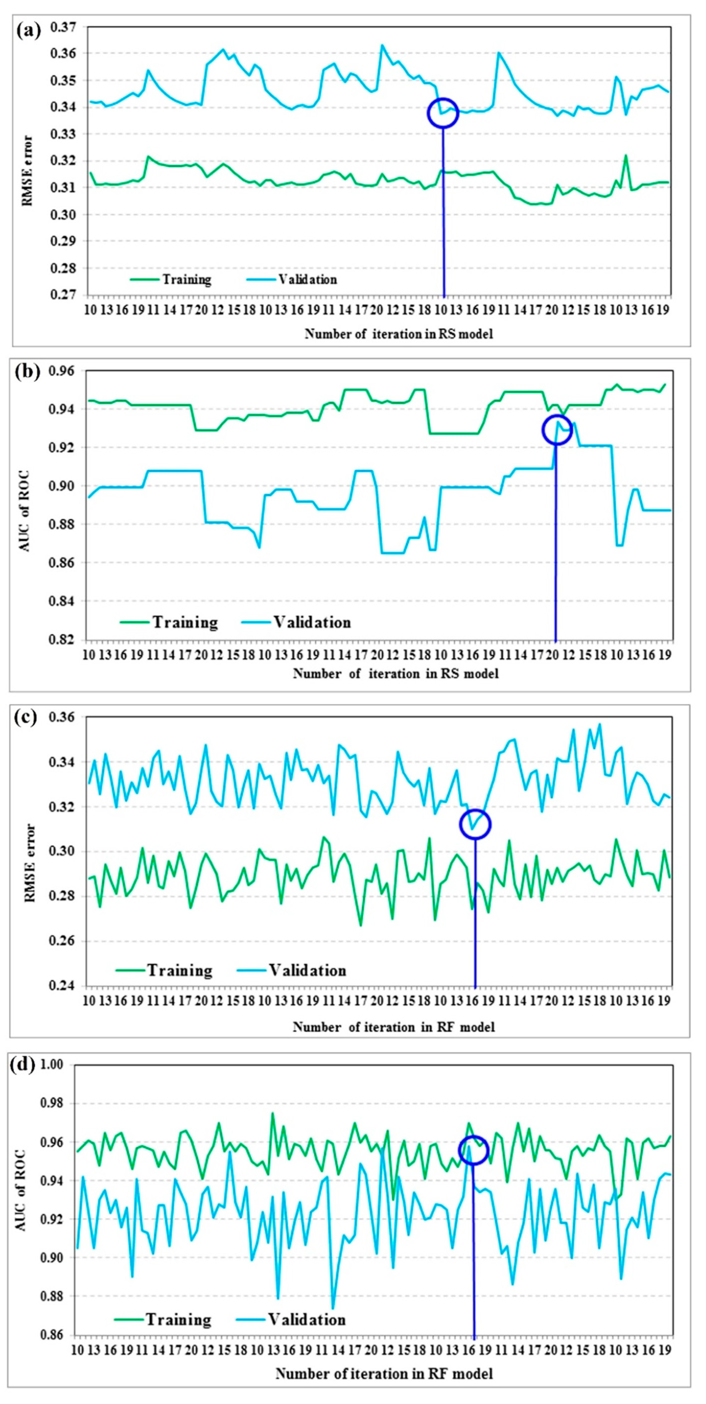
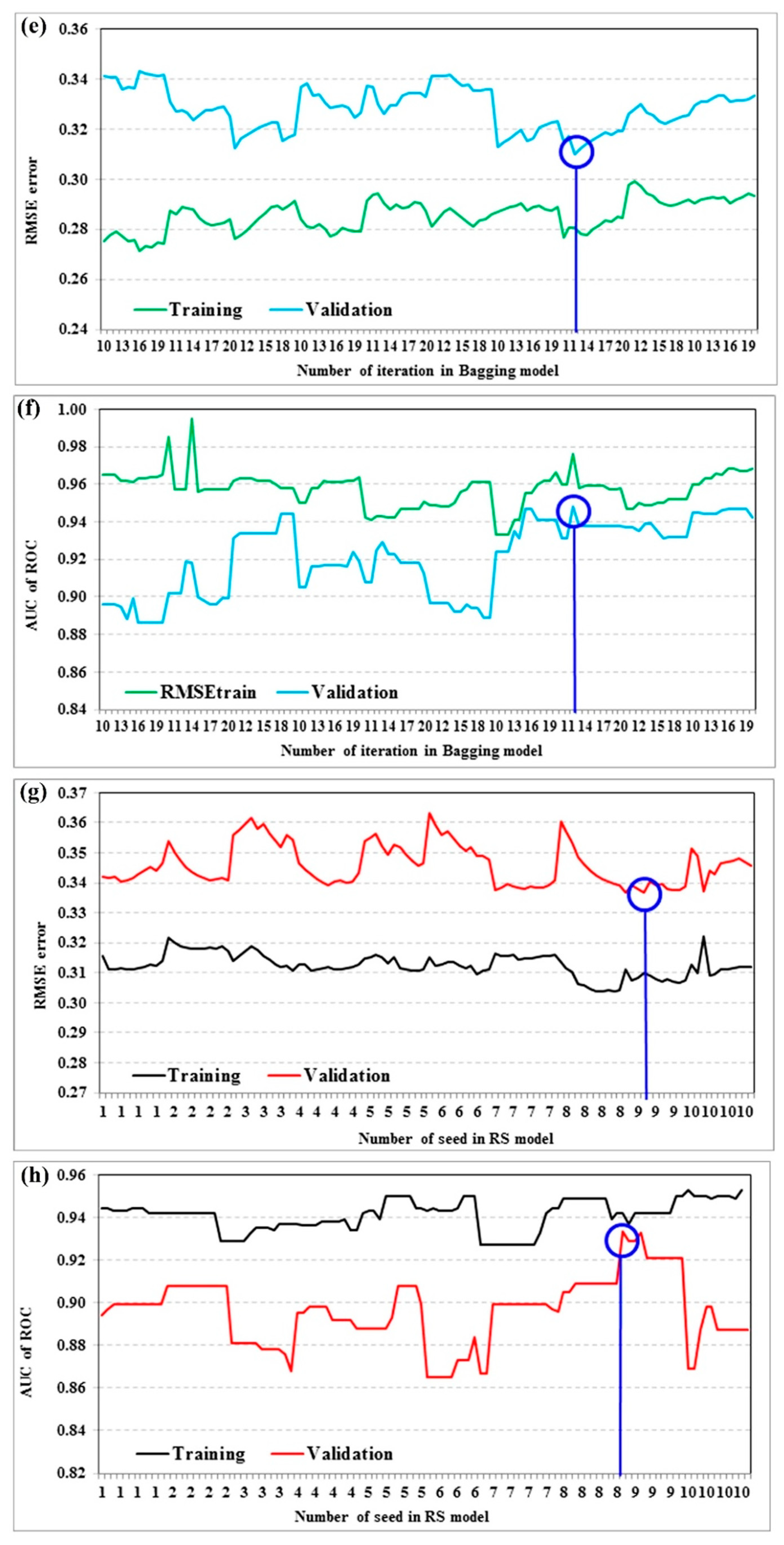
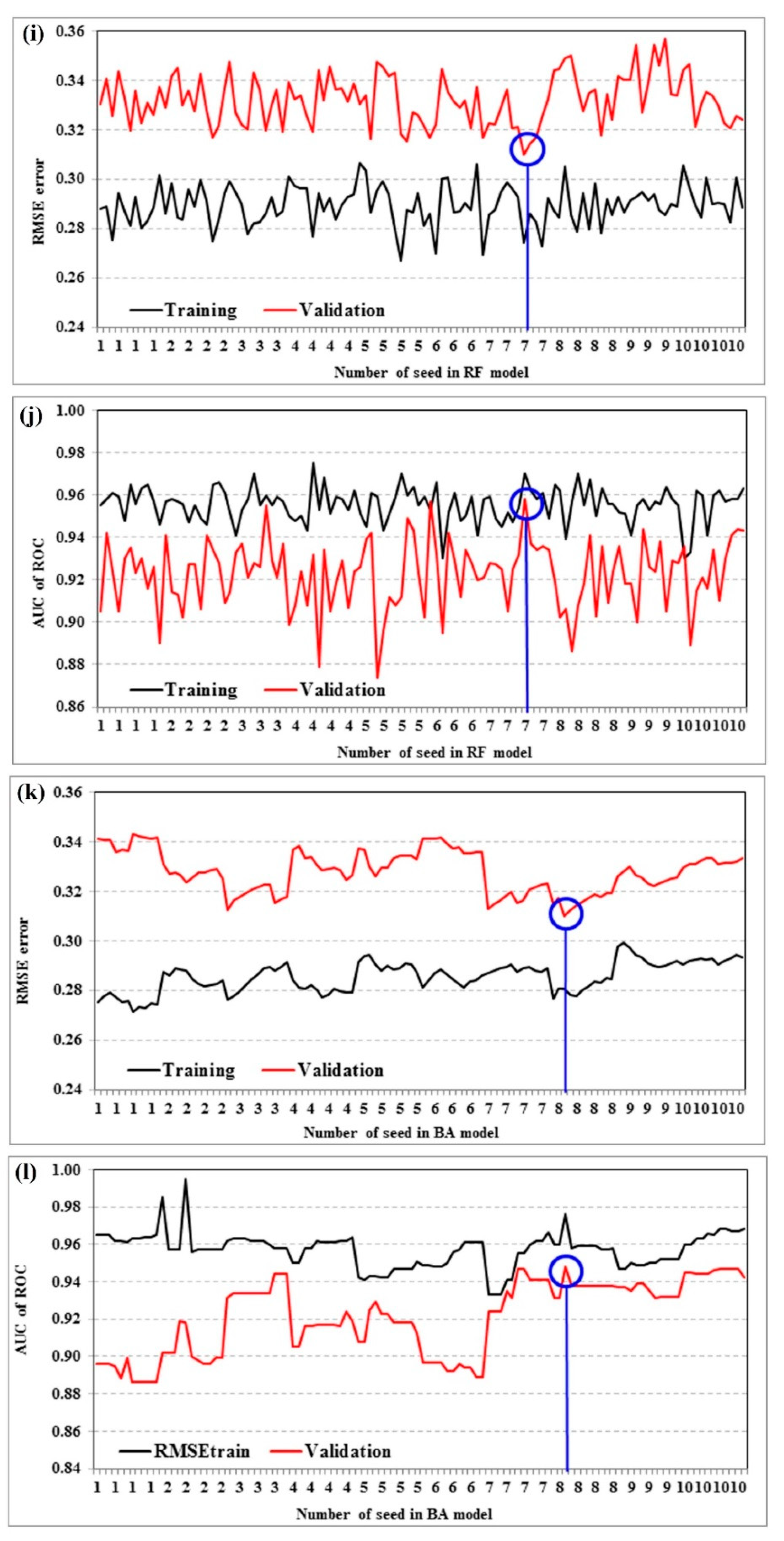
5.2. Modeling Process and Evaluations
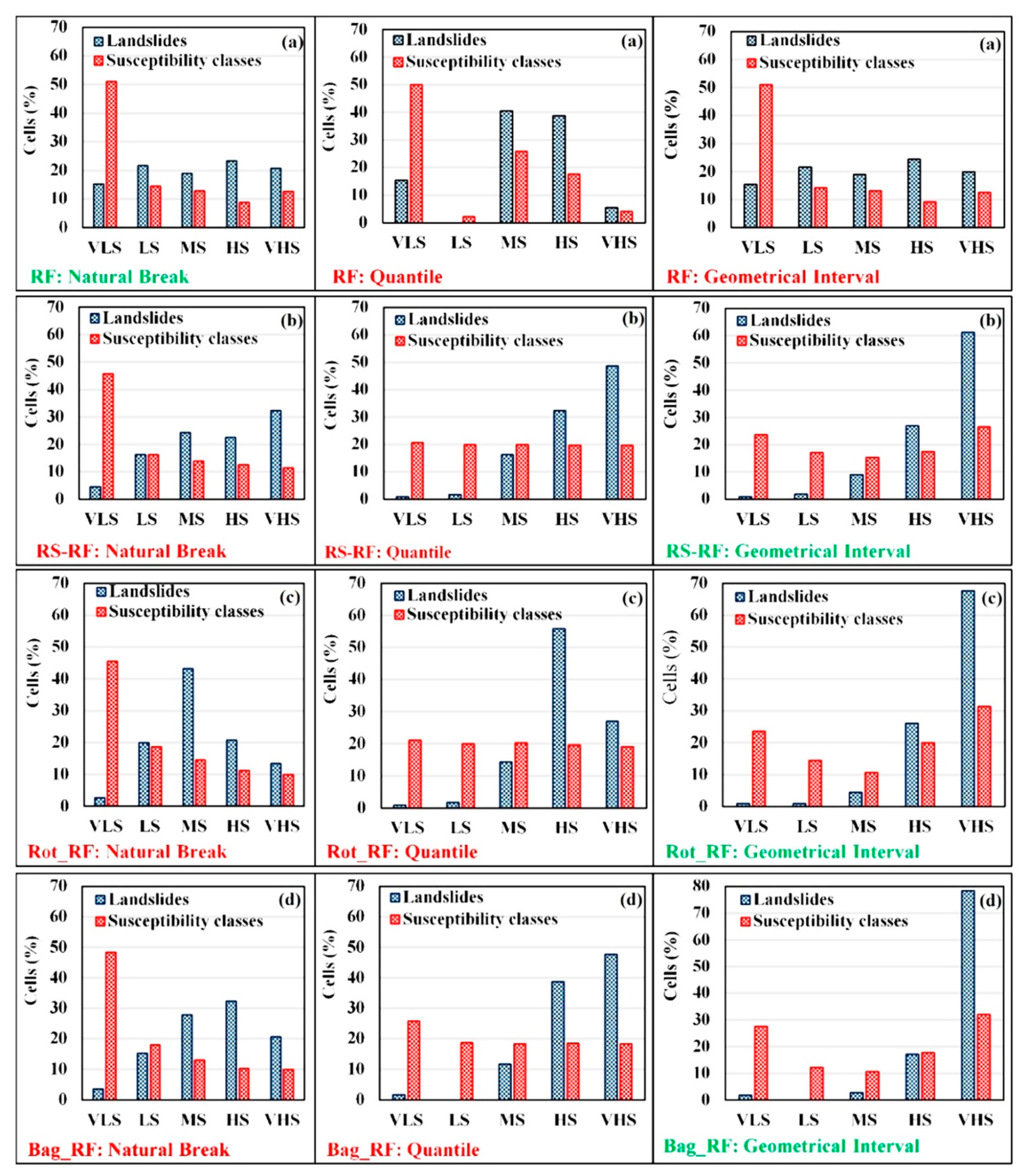
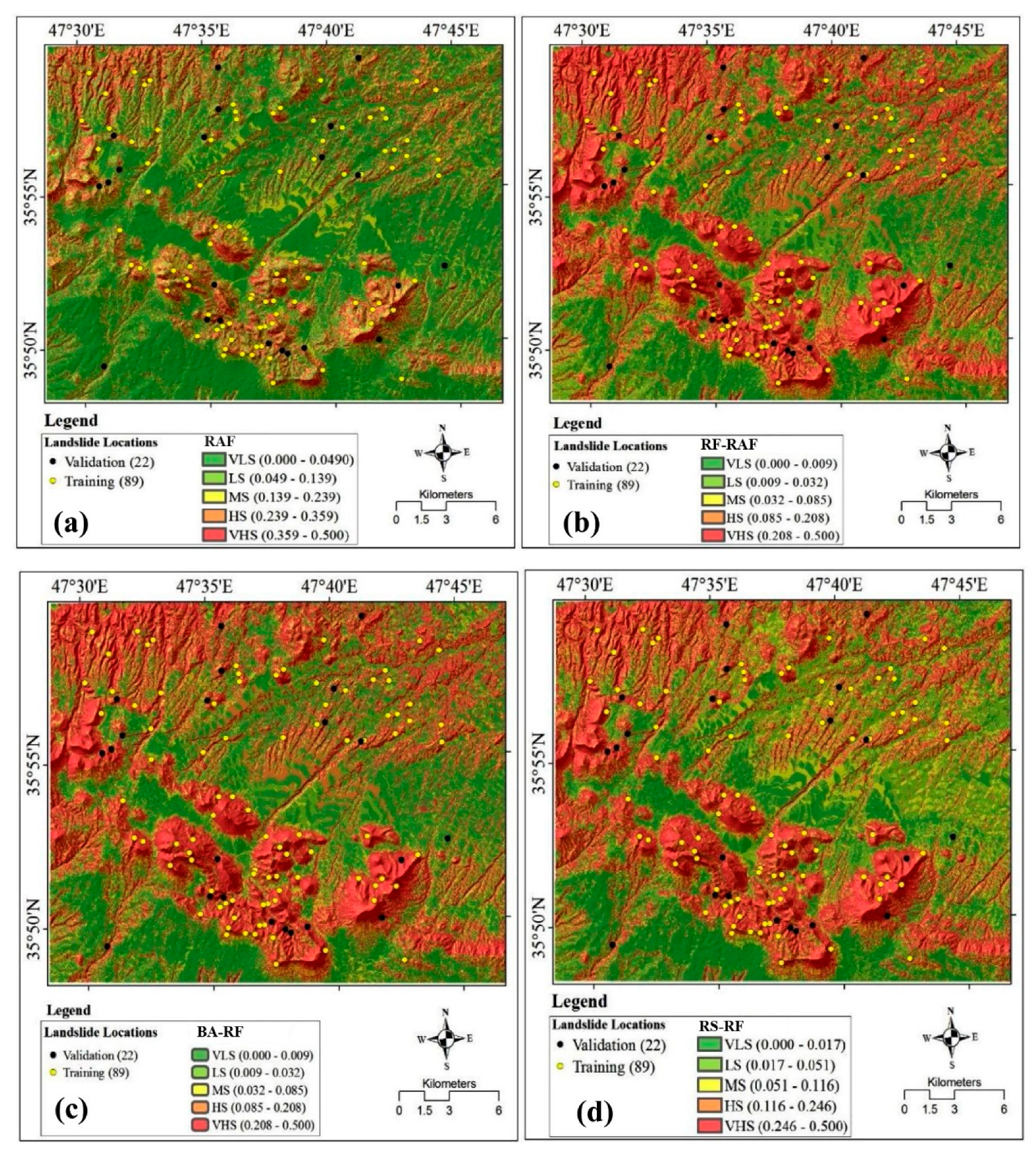
5.3. Preparation of Landslide Susceptibility Maps
5.4. Verification of Landslide Susceptibility Maps
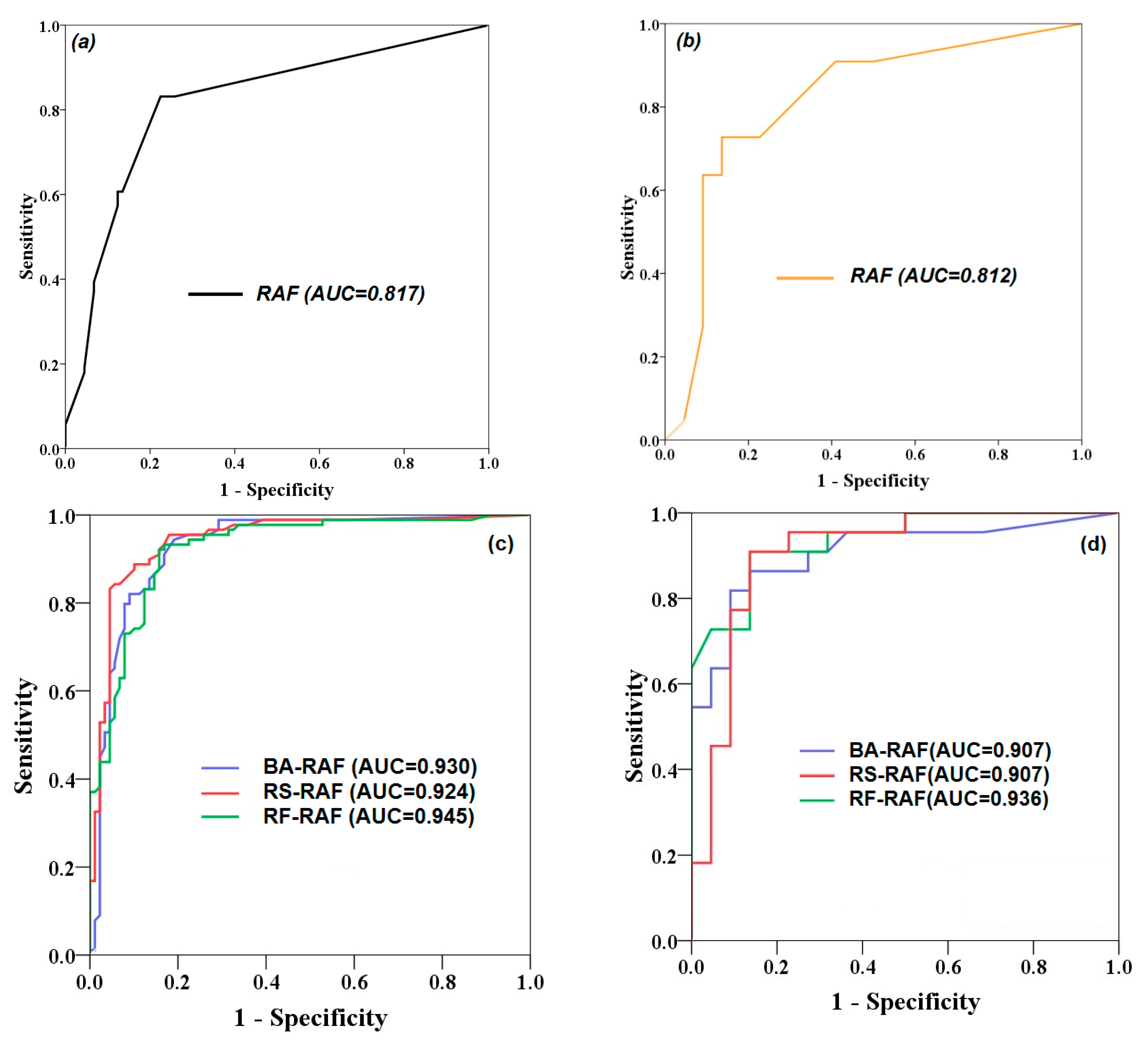
ROC Curve and AUC
6. Discussion
7. Conclusions
Author Contributions
Funding
Conflicts of Interest
References
- Corominas, J.; Moya, J. A review of assessing landslide frequency for hazard zoning purposes. Eng. Geol. 2008, 102, 193–213. [Google Scholar] [CrossRef]
- Piciullo, L.; Calvello, M.; Cepeda, J.M. Territorial early warning systems for rainfall-induced landslides. Earth-Sci. Rev. 2018, 179, 228–247. [Google Scholar] [CrossRef]
- Dao, D.V.; Jaafari, A.; Bayat, M.; Mafi-Gholami, D.; Qi, C.; Moayedi, H.; Phong, T.V.; Ly, H.-B.; Le, T.-T.; Trinh, P.T.; et al. A spatially explicit deep learning neural network model for the prediction of landslide susceptibility. Catena 2020, 188, 104451. [Google Scholar] [CrossRef]
- Yesilnacar, E.; Topal, T. Landslide susceptibility mapping: A comparison of logistic regression and neural networks methods in a medium scale study, hendek region (turkey). Eng. Geol. 2005, 79, 251–266. [Google Scholar] [CrossRef]
- Yilmaz, I. Landslide susceptibility mapping using frequency ratio, logistic regression, artificial neural networks and their comparison: A case study from kat landslides (tokat—turkey). Comput. Geosci. 2009, 35, 1125–1138. [Google Scholar] [CrossRef]
- Pradhan, B. A comparative study on the predictive ability of the decision tree, support vector machine and neuro-fuzzy models in landslide susceptibility mapping using gis. Comput. Geosci. 2013, 51, 350–365. [Google Scholar] [CrossRef]
- Hong, H.; Pradhan, B.; Xu, C.; Tien Bui, D. Spatial prediction of landslide hazard at the yihuang area (china) using two-class kernel logistic regression, alternating decision tree and support vector machines. Catena 2015, 133, 266–281. [Google Scholar] [CrossRef]
- Razavizadeh, S.; Solaimani, K.; Massironi, M.; Kavian, A. Mapping landslide susceptibility with frequency ratio, statistical index, and weights of evidence models: A case study in northern iran. Environ. Earth Sci. 2017, 76, 499. [Google Scholar] [CrossRef]
- Juliev, M.; Mergili, M.; Mondal, I.; Nurtaev, B.; Pulatov, A.; Hübl, J. Comparative analysis of statistical methods for landslide susceptibility mapping in the bostanlik district, uzbekistan. Sci. Total Environ. 2019, 653, 801–814. [Google Scholar] [CrossRef]
- Nhu, V.-H.; Hoang, N.-D.; Nguyen, H.; Ngo, P.T.T.; Bui, T.T.; Hoa, P.V.; Samui, P.; Bui, D.T. Effectiveness assessment of keras based deep learning with different robust optimization algorithms for shallow landslide susceptibility mapping at tropical area. Catena 2020, 188, 104458. [Google Scholar] [CrossRef]
- Thanh, D.Q.; Nguyen, D.H.; Prakash, I.; Jaafari, A.; Nguyen, V.-T.; Van Phong, T.; Pham, B.T. Gis based frequency ratio method for landslide susceptibility mapping at da lat city, lam dong province, vietnam. Vietnam J. Earth Sci. 2020, 42, 55–66. [Google Scholar] [CrossRef] [Green Version]
- Jaafari, A. Lidar-supported prediction of slope failures using an integrated ensemble weights-of-evidence and analytical hierarchy process. Environ. Earth Sci. 2018, 77, 1–42. [Google Scholar] [CrossRef]
- He, Q.; Shahabi, H.; Shirzadi, A.; Li, S.; Chen, W.; Wang, N.; Chai, H.; Bian, H.; Ma, J.; Chen, Y. Landslide spatial modelling using novel bivariate statistical based naïve bayes, rbf classifier, and rbf network machine learning algorithms. Sci. Total Environ. 2019, 663, 1–15. [Google Scholar] [CrossRef] [PubMed]
- Tien Bui, D.; Moayedi, H.; Gör, M.; Jaafari, A.; Foong, L.K. Predicting slope stability failure through machine learning paradigms. ISPRS Int. J. Geo-Inf. 2019, 8, 395. [Google Scholar]
- Moayedi, H.; Tien Bui, D.; Gör, M.; Pradhan, B.; Jaafari, A. The feasibility of three prediction techniques of the artificial neural network, adaptive neuro-fuzzy inference system, and hybrid particle swarm optimization for assessing the safety factor of cohesive slopes. ISPRS Int. J. Geo-Inf. 2019, 8, 391. [Google Scholar] [CrossRef] [Green Version]
- Pham, B.T.; Prakash, I.; Jaafari, A.; Bui, D.T. Spatial prediction of rainfall-induced landslides using aggregating one-dependence estimators classifier. J. Indian Soc. Remote Sens. 2018, 46, 1457–1470. [Google Scholar] [CrossRef]
- Jaafari, A.; Rezaeian, J.; Omrani, M.S. Spatial prediction of slope failures in support of forestry operations safety. Croat. J. For. Eng. 2017, 38, 107–118. [Google Scholar]
- Wang, Y.; Hong, H.; Chen, W.; Li, S.; Panahi, M.; Khosravi, K.; Shirzadi, A.; Shahabi, H.; Panahi, S.; Costache, R. Flood susceptibility mapping in dingnan county (china) using adaptive neuro-fuzzy inference system with biogeography based optimization and imperialistic competitive algorithm. J. Environ. Manag. 2019, 247, 712–729. [Google Scholar] [CrossRef]
- Khosravi, K.; Shahabi, H.; Pham, B.T.; Adamowski, J.; Shirzadi, A.; Pradhan, B.; Dou, J.; Ly, H.-B.; Gróf, G.; Ho, H.L. A comparative assessment of flood susceptibility modeling using multi-criteria decision-making analysis and machine learning methods. J. Hydrol. 2019, 573, 311–323. [Google Scholar] [CrossRef]
- Chen, W.; Hong, H.; Li, S.; Shahabi, H.; Wang, Y.; Wang, X.; Ahmad, B.B. Flood susceptibility modelling using novel hybrid approach of reduced-error pruning trees with bagging and random subspace ensembles. J. Hydrol. 2019, 575, 864–873. [Google Scholar] [CrossRef]
- Pham, B.T.; Nguyen, M.D.; Dao, D.V.; Prakash, I.; Ly, H.B.; Le, T.T.; Ho, L.S.; Nguyen, K.T.; Ngo, T.Q.; Hoang, V.; et al. Development of artificial intelligence models for the prediction of compression coefficient of soil: An application of monte carlo sensitivity analysis. Sci. Total Environ. 2019, 679, 172–184. [Google Scholar] [CrossRef]
- Tien Bui, D.; Shahabi, H.; Shirzadi, A.; Chapi, K.; Hoang, N.-D.; Pham, B.; Bui, Q.-T.; Tran, C.-T.; Panahi, M.; Bin Ahamd, B. A novel integrated approach of relevance vector machine optimized by imperialist competitive algorithm for spatial modeling of shallow landslides. Remote Sens. 2018, 10, 1538. [Google Scholar] [CrossRef] [Green Version]
- Tien Bui, D.; Khosravi, K.; Li, S.; Shahabi, H.; Panahi, M.; Singh, V.; Chapi, K.; Shirzadi, A.; Panahi, S.; Chen, W. New hybrids of anfis with several optimization algorithms for flood susceptibility modeling. Water 2018, 10, 1210. [Google Scholar] [CrossRef] [Green Version]
- Shafizadeh-Moghadam, H.; Valavi, R.; Shahabi, H.; Chapi, K.; Shirzadi, A. Novel forecasting approaches using combination of machine learning and statistical models for flood susceptibility mapping. J. Environ. Manag. 2018, 217, 1–11. [Google Scholar] [CrossRef] [PubMed] [Green Version]
- Chapi, K.; Singh, V.P.; Shirzadi, A.; Shahabi, H.; Bui, D.T.; Pham, B.T.; Khosravi, K. A novel hybrid artificial intelligence approach for flood susceptibility assessment. Environ. Model. Softw. 2017, 95, 229–245. [Google Scholar] [CrossRef]
- Chen, W.; Li, Y.; Xue, W.; Shahabi, H.; Li, S.; Hong, H.; Wang, X.; Bian, H.; Zhang, S.; Pradhan, B. Modeling flood susceptibility using data-driven approaches of naïve bayes tree, alternating decision tree, and random forest methods. Sci. Total Environ. 2020, 701, 134979. [Google Scholar] [CrossRef] [PubMed]
- Shahabi, H.; Shirzadi, A.; Ghaderi, K.; Omidvar, E.; Al-Ansari, N.; Clague, J.J.; Geertsema, M.; Khosravi, K.; Amini, A.; Bahrami, S. Flood detection and susceptibility mapping using sentinel-1 remote sensing data and a machine learning approach: Hybrid intelligence of bagging ensemble based on k-nearest neighbor classifier. Remote Sens. 2020, 12, 266. [Google Scholar] [CrossRef] [Green Version]
- Khosravi, K.; Melesse, A.M.; Shahabi, H.; Shirzadi, A.; Chapi, K.; Hong, H. Flood susceptibility mapping at ningdu catchment, china using bivariate and data mining techniques. In Extreme Hydrology and Climate Variability; Elsevier: Amsterdam, The Netherlands, 2019; pp. 419–434. [Google Scholar]
- Jaafari, A.; Zenner, E.K.; Panahi, M.; Shahabi, H. Hybrid artificial intelligence models based on a neuro-fuzzy system and metaheuristic optimization algorithms for spatial prediction of wildfire probability. Agric. For. Meteorol. 2019, 266, 198–207. [Google Scholar] [CrossRef]
- Jaafari, A.; Pourghasemi, H.R. Factors influencing regional-scale wildfire probability in iran: An application of random forest and support vector machine. In Spatial Modeling in Gis and R for Earth and Environmental Sciences; Elsevier: Amsterdam, The Netherlands, 2019; pp. 607–619. [Google Scholar]
- Taheri, K.; Shahabi, H.; Chapi, K.; Shirzadi, A.; Gutiérrez, F.; Khosravi, K. Sinkhole susceptibility mapping: A comparison between bayes-based machine learning algorithms. Land Degrad. Dev. 2019, 30, 730–745. [Google Scholar] [CrossRef]
- Roodposhti, M.S.; Safarrad, T.; Shahabi, H. Drought sensitivity mapping using two one-class support vector machine algorithms. Atmos. Res. 2017, 193, 73–82. [Google Scholar] [CrossRef]
- Choubin, B.; Soleimani, F.; Pirnia, A.; Sajedi-Hosseini, F.; Alilou, H.; Rahmati, O.; Melesse, A.M.; Singh, V.P.; Shahabi, H. Effects of drought on vegetative cover changes: Investigating spatiotemporal patterns. In Extreme Hydrology and Climate Variability; Elsevier: Amsterdam, The Netherlands, 2019; pp. 213–222. [Google Scholar]
- Lee, S.; Panahi, M.; Pourghasemi, H.R.; Shahabi, H.; Alizadeh, M.; Shirzadi, A.; Khosravi, K.; Melesse, A.M.; Yekrangnia, M.; Rezaie, F. Sevucas: A novel gis-based machine learning software for seismic vulnerability assessment. Appl. Sci. 2019, 9, 3495. [Google Scholar] [CrossRef] [Green Version]
- Alizadeh, M.; Alizadeh, E.; Asadollahpour Kotenaee, S.; Shahabi, H.; Beiranvand Pour, A.; Panahi, M.; Bin Ahmad, B.; Saro, L. Social vulnerability assessment using artificial neural network (ann) model for earthquake hazard in tabriz city, iran. Sustainability 2018, 10, 3376. [Google Scholar] [CrossRef] [Green Version]
- Azareh, A.; Rahmati, O.; Rafiei-Sardooi, E.; Sankey, J.B.; Lee, S.; Shahabi, H.; Ahmad, B.B. Modelling gully-erosion susceptibility in a semi-arid region, iran: Investigation of applicability of certainty factor and maximum entropy models. Sci. Total Environ. 2019, 655, 684–696. [Google Scholar] [CrossRef] [PubMed]
- Tien Bui, D.; Shirzadi, A.; Shahabi, H.; Chapi, K.; Omidavr, E.; Pham, B.T.; Talebpour Asl, D.; Khaledian, H.; Pradhan, B.; Panahi, M. A novel ensemble artificial intelligence approach for gully erosion mapping in a semi-arid watershed (iran). Sensors 2019, 19, 2444. [Google Scholar] [CrossRef] [PubMed] [Green Version]
- Tien Bui, D.; Shahabi, H.; Shirzadi, A.; Chapi, K.; Pradhan, B.; Chen, W.; Khosravi, K.; Panahi, M.; Bin Ahmad, B.; Saro, L. Land subsidence susceptibility mapping in south korea using machine learning algorithms. Sensors 2018, 18, 2464. [Google Scholar] [CrossRef] [Green Version]
- Rahmati, O.; Samadi, M.; Shahabi, H.; Azareh, A.; Rafiei-Sardooi, E.; Alilou, H.; Melesse, A.M.; Pradhan, B.; Chapi, K.; Shirzadi, A. Swpt: An automated gis-based tool for prioritization of sub-watersheds based on morphometric and topo-hydrological factors. Geosci. Front. 2019, 10, 2167–2175. [Google Scholar] [CrossRef]
- Pham, B.T.; Jaafari, A.; Prakash, I.; Singh, S.K.; Quoc, N.K.; Bui, D.T. Hybrid computational intelligence models for groundwater potential mapping. Catena 2019, 182, 104101. [Google Scholar] [CrossRef]
- Tien Bui, D.; Shahabi, H.; Omidvar, E.; Shirzadi, A.; Geertsema, M.; Clague, J.J.; Khosravi, K.; Pradhan, B.; Pham, B.T.; Chapi, K. Shallow landslide prediction using a novel hybrid functional machine learning algorithm. Remote Sens. 2019, 11, 931. [Google Scholar] [CrossRef] [Green Version]
- Pham, B.T.; Prakash, I.; Dou, J.; Singh, S.K.; Trinh, P.T.; Tran, H.T.; Le, T.M.; Van Phong, T.; Khoi, D.K.; Shirzadi, A. A novel hybrid approach of landslide susceptibility modelling using rotation forest ensemble and different base classifiers. Geocarto Int. 2019. [Google Scholar] [CrossRef]
- Nguyen, V.V.; Pham, B.T.; Vu, B.T.; Prakash, I.; Jha, S.; Shahabi, H.; Shirzadi, A.; Ba, D.N.; Kumar, R.; Chatterjee, J.M. Hybrid machine learning approaches for landslide susceptibility modeling. Forests 2019, 10, 157. [Google Scholar] [CrossRef] [Green Version]
- Nguyen, P.T.; Tuyen, T.T.; Shirzadi, A.; Pham, B.T.; Shahabi, H.; Omidvar, E.; Amini, A.; Entezami, H.; Prakash, I.; Phong, T.V. Development of a novel hybrid intelligence approach for landslide spatial prediction. Appl. Sci. 2019, 9, 2824. [Google Scholar] [CrossRef] [Green Version]
- Shirzadi, A.; Solaimani, K.; Roshan, M.H.; Kavian, A.; Chapi, K.; Shahabi, H.; Keesstra, S.; Ahmad, B.B.; Bui, D.T. Uncertainties of prediction accuracy in shallow landslide modeling: Sample size and raster resolution. Catena 2019, 178, 172–188. [Google Scholar] [CrossRef]
- Nhu, V.H.; Rahmati, O.; Falah, F.; Shojaei, S.; Al-Ansari, N.; Shahabi, H.; Shirzadi, A.; Górski, K.; Nguyen, H.; Ahmad, B.B. Mapping of Groundwater Spring Potential in Karst Aquifer System Using Novel Ensemble Bivariate and Multivariate Models. Water 2020, 12, 985. [Google Scholar] [CrossRef] [Green Version]
- Pham, B.T.; Tien Bui, D.; Prakash, I.; Dholakia, M.B. Hybrid integration of multilayer perceptron neural networks and machine learning ensembles for landslide susceptibility assessment at himalayan area (india) using gis. Catena 2017, 149, 52–63. [Google Scholar] [CrossRef]
- Pham, B.T.; Shirzadi, A.; Shahabi, H.; Omidvar, E.; Singh, S.K.; Sahana, M.; Asl, D.T.; Ahmad, B.B.; Quoc, N.K.; Lee, S. Landslide susceptibility assessment by novel hybrid machine learning algorithms. Sustainability 2019, 11, 4386. [Google Scholar] [CrossRef] [Green Version]
- Pham, B.T.; Jaafari, A.; Prakash, I.; Bui, D.T. A novel hybrid intelligent model of support vector machines and the multiboost ensemble for landslide susceptibility modeling. Bull. Eng. Geol. Environ. 2019, 78, 2865–2886. [Google Scholar] [CrossRef]
- Hong, H.; Liu, J.; Bui, D.T.; Pradhan, B.; Acharya, T.D.; Pham, B.T.; Zhu, A.-X.; Chen, W.; Ahmad, B.B. Landslide susceptibility mapping using j48 decision tree with adaboost, bagging and rotation forest ensembles in the guangchang area (china). Catena 2018, 163, 399–413. [Google Scholar] [CrossRef]
- Shirzadi, A.; Bui, D.T.; Pham, B.T.; Solaimani, K.; Chapi, K.; Kavian, A.; Shahabi, H.; Revhaug, I. Shallow landslide susceptibility assessment using a novel hybrid intelligence approach. Environ. Earth Sci. 2017, 76, 60. [Google Scholar] [CrossRef]
- Chen, W.; Shirzadi, A.; Shahabi, H.; Ahmad, B.B.; Zhang, S.; Hong, H.; Zhang, N. A novel hybrid artificial intelligence approach based on the rotation forest ensemble and naïve bayes tree classifiers for a landslide susceptibility assessment in langao county, china. Geomat. Nat. Hazards Risk 2017, 8, 1955–1977. [Google Scholar] [CrossRef] [Green Version]
- Abedini, M.; Ghasemian, B.; Shirzadi, A.; Shahabi, H.; Chapi, K.; Pham, B.T.; Bin Ahmad, B.; Tien Bui, D. A novel hybrid approach of bayesian logistic regression and its ensembles for landslide susceptibility assessment. Geocarto Int. 2018, 34, 1427–1457. [Google Scholar] [CrossRef]
- Miraki, S.; Zanganeh, S.H.; Chapi, K.; Singh, V.P.; Shirzadi, A.; Shahabi, H.; Pham, B.T. Mapping groundwater potential using a novel hybrid intelligence approach. Water Resour. Manag. 2019, 33, 281–302. [Google Scholar] [CrossRef]
- Arabameri, A.; Chen, W.; Blaschke, T.; Tiefenbacher, J.P.; Pradhan, B.; Tien Bui, D. Gully head-cut distribution modeling using machine learning methods—A case study of nw iran. Water 2020, 12, 16. [Google Scholar] [CrossRef] [Green Version]
- Ahmadlou, M.; Karimi, M.; Alizadeh, S.; Shirzadi, A.; Parvinnejhad, D.; Shahabi, H.; Panahi, M. Flood susceptibility assessment using integration of adaptive network-based fuzzy inference system (ANFIS) and biogeography-based optimization (BBO) and BAT algorithms (BA). Geocarto Int 2019, 34, 1252–1272. [Google Scholar] [CrossRef]
- Galli, M.; Ardizzone, F.; Cardinali, M.; Guzzetti, F.; Reichenbach, P. Comparing landslide inventory maps. Geomorphology 2008, 94, 268–289. [Google Scholar] [CrossRef]
- Guzzetti, F.; Carrara, A.; Cardinali, M.; Reichenbach, P. Landslide hazard evaluation: A review of current techniques and their application in a multi-scale study, central italy. Geomorphology 1999, 31, 181–216. [Google Scholar] [CrossRef]
- Shirzadi, A.; Chapi, K.; Shahabi, H.; Solaimani, K.; Kavian, A.; Ahmad, B.B. Rock fall susceptibility assessment along a mountainous road: An evaluation of bivariate statistic, analytical hierarchy process and frequency ratio. Environ. Earth Sci. 2017, 76, 152. [Google Scholar] [CrossRef]
- Shirzadi, A.; Soliamani, K.; Habibnejhad, M.; Kavian, A.; Chapi, K.; Shahabi, H.; Chen, W.; Khosravi, K.; Thai Pham, B.; Pradhan, B. Novel gis based machine learning algorithms for shallow landslide susceptibility mapping. Sensors 2018, 18, 3777. [Google Scholar] [CrossRef] [PubMed]
- Chen, W.; Zhao, X.; Shahabi, H.; Shirzadi, A.; Khosravi, K.; Chai, H.; Zhang, S.; Zhang, L.; Ma, J.; Chen, Y.; et al. Spatial prediction of landslide susceptibility by combining evidential belief function, logistic regression and logistic model tree. Geocarto Int 2019, 34, 1177–1201. [Google Scholar] [CrossRef]
- Pham, B.T.; Prakash, I.; Singh, S.K.; Shirzadi, A.; Shahabi, H.; Bui, D.T. Landslide susceptibility modeling using reduced error pruning trees and different ensemble techniques: Hybrid machine learning approaches. Catena 2019, 175, 203–218. [Google Scholar] [CrossRef]
- Dehnavi, A.; Aghdam, I.N.; Pradhan, B.; Varzandeh, M.H.M. A new hybrid model using step-wise weight assessment ratio analysis (swara) technique and adaptive neuro-fuzzy inference system (anfis) for regional landslide hazard assessment in iran. Catena 2015, 135, 122–148. [Google Scholar] [CrossRef]
- Froude, M.J.; Petley, D. Global fatal landslide occurrence from 2004 to 2016. Nat. Hazards Earth Syst. Sci. 2018, 18, 2161–2181. [Google Scholar] [CrossRef] [Green Version]
- Nefeslioglu, H.A.; Duman, T.Y.; Durmaz, S. Landslide susceptibility mapping for a part of tectonic kelkit valley (eastern black sea region of turkey). Geomorphology 2008, 94, 401–418. [Google Scholar] [CrossRef]
- Kavzoglu, T.; Sahin, E.K.; Colkesen, I. An assessment of multivariate and bivariate approaches in landslide susceptibility mapping: A case study of duzkoy district. Nat. Hazards 2015, 76, 471–496. [Google Scholar] [CrossRef]
- Pham, B.T.; Bui, D.T.; Pourghasemi, H.R.; Indra, P.; Dholakia, M. Landslide susceptibility assesssment in the uttarakhand area (india) using gis: A comparison study of prediction capability of naïve bayes, multilayer perceptron neural networks, and functional trees methods. Theor. Appl. Climatol. 2017, 128, 255–273. [Google Scholar] [CrossRef]
- Pham, B.T.; Pradhan, B.; Bui, D.T.; Prakash, I.; Dholakia, M. A comparative study of different machine learning methods for landslide susceptibility assessment: A case study of uttarakhand area (india). Environ. Model. Softw. 2016, 84, 240–250. [Google Scholar] [CrossRef]
- He, S.; Ouyang, C.; Luo, Y. Seismic stability analysis of soil nail reinforced slope using kinematic approach of limit analysis. Environ. Earth Sci. 2012, 66, 319–326. [Google Scholar] [CrossRef]
- Gorsevski, P.V.; Jankowski, P. An optimized solution of multi-criteria evaluation analysis of landslide susceptibility using fuzzy sets and kalman filter. Comput. Geosci. 2010, 36, 1005–1020. [Google Scholar] [CrossRef]
- Oh, H.-J.; Pradhan, B. Application of a neuro-fuzzy model to landslide-susceptibility mapping for shallow landslides in a tropical hilly area. Comput. Geosci. 2011, 37, 1264–1276. [Google Scholar] [CrossRef]
- Ercanoglu, M.; Gokceoglu, C. Assessment of landslide susceptibility for a landslide-prone area (north of yenice, nw turkey) by fuzzy approach. Environ. Geol. 2002, 41, 720–730. [Google Scholar]
- Atkinson, P.M.; Massari, R. Autologistic modelling of susceptibility to landsliding in the central apennines, italy. Geomorphology 2011, 130, 55–64. [Google Scholar] [CrossRef]
- Hengl, T.; Gruber, S.; Shrestha, D. Digital Terrain Analysis in Ilwis; International Institute for Geo-Information Science and Earth Observation: Enschede, The Netherlands, 2003; p. 62. [Google Scholar]
- Talebi, A.; Uijlenhoet, R.; Troch, P.A. Soil moisture storage and hillslope stability. Nat. Hazards Earth Syst. Sci. 2007, 7, 523–534. [Google Scholar] [CrossRef] [Green Version]
- Pourghasemi, H.R.; Jirandeh, A.G.; Pradhan, B.; Xu, C.; Gokceoglu, C. Landslide susceptibility mapping using support vector machine and gis at the golestan province, iran. J. Earth Syst. Sci. 2013, 122, 349–369. [Google Scholar] [CrossRef] [Green Version]
- Moore, I.; Burch, G. Sediment transport capacity of sheet and rill flow: Application of unit stream power theory. Water Resour. Res. 1986, 22, 1350–1360. [Google Scholar] [CrossRef]
- Iqbal, M. An Introduction to Solar Radiation; Elsevier: Amsterdam, The Netherlands, 2012. [Google Scholar]
- Regmi, N.R.; Giardino, J.R.; McDonald, E.V.; Vitek, J.D. A comparison of logistic regression-based models of susceptibility to landslides in western colorado, USA. Landslides 2014, 11, 247–262. [Google Scholar] [CrossRef]
- Moore, I.D.; Grayson, R.; Ladson, A. Digital terrain modelling: A review of hydrological, geomorphological, and biological applications. Hydrol. Process. 1991, 5, 3–30. [Google Scholar] [CrossRef]
- Wilson, J.P.; Gallant, J.C. Terrain analysis: Principles and Applications; John Wiley & Sons: Hoboken, NJ, USA, 2000. [Google Scholar]
- Park, S.; Choi, C.; Kim, B.; Kim, J. Landslide susceptibility mapping using frequency ratio, analytic hierarchy process, logistic regression, and artificial neural network methods at the inje area, korea. Environ. Earth Sci. 2013, 68, 1443–1464. [Google Scholar] [CrossRef]
- Chowdhury, R.; Flentje, P.; Bhattacharya, G. Geotechnics in the Twenty-First Century, Uncertainties and Other Challenges: With Particular Reference to Landslide Hazard and Risk Assessment. In Proceedings of the International Symposium on Engineering under Uncertainty: Safety Assessment and Management (ISEUSAM-2012); Springer: New Delhi, India, 2013; pp. 27–53. [Google Scholar]
- Cevik, E.; Topal, T. Gis-based landslide susceptibility mapping for a problematic segment of the natural gas pipeline, hendek (turkey). Environ. Geol. 2003, 44, 949–962. [Google Scholar] [CrossRef]
- Nampak, H.; Pradhan, B.; Manap, M.A. Application of gis based data driven evidential belief function model to predict groundwater potential zonation. J. Hydrol. 2014, 513, 283–300. [Google Scholar] [CrossRef]
- Barlow, J.; Martin, Y.; Franklin, S. Detecting translational landslide scars using segmentation of landsat etm+ and dem data in the northern cascade mountains, british columbia. Can. J. Remote Sens. 2003, 29, 510–517. [Google Scholar] [CrossRef]
- Yang, W.; Wang, M.; Shi, P. Using modis ndvi time series to identify geographic patterns of landslides in vegetated regions. IEEE Geosci. Remote Sens. Lett. 2012, 10, 707–710. [Google Scholar] [CrossRef]
- Hong, H.; Shahabi, H.; Shirzadi, A.; Chen, W.; Chapi, K.; Ahmad, B.B.; Roodposhti, M.S.; Hesar, A.Y.; Tian, Y.; Bui, D.T. Landslide susceptibility assessment at the wuning area, china: A comparison between multi-criteria decision making, bivariate statistical and machine learning methods. Nat. Hazards 2019, 96, 173–212. [Google Scholar] [CrossRef]
- Demir, G.; Aytekin, M.; Akgun, A. Landslide susceptibility mapping by frequency ratio and logistic regression methods: An example from niksar–resadiye (tokat, turkey). Arab. J. Geosci. 2015, 8, 1801–1812. [Google Scholar] [CrossRef]
- Donati, L.; Turrini, M.C. An objective method to rank the importance of the factors predisposing to landslides with the gis methodology: Application to an area of the apennines (valnerina; perugia, italy). Eng. Geol. 2002, 63, 277–289. [Google Scholar] [CrossRef]
- Breiman, L.; Friedman, J.; Olshen, R.; Stone, C. Classification and Regression Trees; CRC Press: Boca Raton, FL, USA, 1984; Volume 37, pp. 237–251. [Google Scholar]
- Kim, J.-C.; Lee, S.; Jung, H.-S.; Lee, S. Landslide susceptibility mapping using random forest and boosted tree models in pyeong-chang, korea. Geocarto Int. 2018, 33, 1000–1015. [Google Scholar] [CrossRef]
- Breiman, L. Random forests. Mach. Learn. 2001, 45, 5–32. [Google Scholar] [CrossRef] [Green Version]
- Micheletti, N.; Foresti, L.; Robert, S.; Leuenberger, M.; Pedrazzini, A.; Jaboyedoff, M.; Kanevski, M. Machine learning feature selection methods for landslide susceptibility mapping. Math. Geosci. 2014, 46, 33–57. [Google Scholar] [CrossRef] [Green Version]
- Svetnik, V.; Liaw, A.; Tong, C.; Culberson, J.C.; Sheridan, R.P.; Feuston, B.P. Random forest: A classification and regression tool for compound classification and qsar modeling. J. Chem. Inf. Comput. Sci. 2003, 43, 1947–1958. [Google Scholar] [CrossRef]
- Polikar, R. Ensemble based systems in decision making. IEEE Circuits Syst. Mag. 2006, 6, 21–45. [Google Scholar] [CrossRef]
- Rokach, L. Ensemble-based classifiers. Artif. Intell. Rev. 2010, 33, 1–39. [Google Scholar] [CrossRef]
- Opitz, D.; Maclin, R. Popular ensemble methods: An empirical study. J. Artif. Intell. Res. 1999, 11, 169–198. [Google Scholar] [CrossRef]
- Breiman, L. Bagging predictors. Mach. Learn. 1996, 24, 123–140. [Google Scholar] [CrossRef] [Green Version]
- Breiman, L. Arcing the Edge; Technical Report 486; Statistics Department, University of California at Berkeley: Berkeley, CA, USA, 1997. [Google Scholar]
- Schapire, R.E.; Freund, Y.; Bartlett, P.; Lee, W.S. Boosting the margin: A new explanation for the effectiveness of voting methods. Ann. Stat. 1998, 26, 1651–1686. [Google Scholar] [CrossRef]
- Kleinberg, E.M. On the algorithmic implementation of stochastic discrimination. Ieee Trans. Pattern Anal. Mach. Intell. 2000, 22, 473–490. [Google Scholar] [CrossRef]
- Ho, T.K. The random subspace method for constructing decision forests. IEEE Trans. Pattern Anal. Mach. Intell. 1998, 20, 832–844. [Google Scholar]
- Wang, X.; Tang, X. Random sampling for subspace face recognition. Int. J. Comput. Vis. 2006, 70, 91–104. [Google Scholar] [CrossRef]
- Rodriguez, J.J.; Kuncheva, L.I.; Alonso, C.J. Rotation forest: A new classifier ensemble method. IEEE Trans. Pattern Anal. Mach. Intell. 2006, 28, 1619–1630. [Google Scholar] [CrossRef]
- Caruana, R.; Niculescu-Mizil, A. Data Mining in Metric Space: An Empirical Analysis of Supervised Learning Performance Criteria. In Proceedings of the Tenth ACM SIGKDD International Conference on Knowledge Discovery and Data Mining, Seattle, WA, USA, 22–25 August 2004; pp. 69–78. [Google Scholar]
- Lavesson, N.; Davidsson, P. Generic Methods for Multi-Criteria Evaluation. In Proceedings of the 2008 SIAM International Conference on Data Mining, Atlanta, GA, USA, 24–26 April 2008; pp. 541–546. [Google Scholar]
- Tien Bui, D.; Shirzadi, A.; Shahabi, H.; Geertsema, M.; Omidvar, E.; Clague, J.J.; Thai Pham, B.; Dou, J.; Talebpour Asl, D.; Bin Ahmad, B. New ensemble models for shallow landslide susceptibility modeling in a semi-arid watershed. Forests 2019, 10, 743. [Google Scholar] [CrossRef] [Green Version]
- Kumar, R.; Indrayan, A. Receiver operating characteristic (roc) curve for medical researchers. Indian Pediatrics 2011, 48, 277–287. [Google Scholar] [CrossRef]
- Akobeng, A.K. Understanding diagnostic tests 3: Receiver operating characteristic curves. Acta Paediatr. 2007, 96, 644–647. [Google Scholar] [CrossRef]
- Wang, G.; Lei, X.; Chen, W.; Shahabi, H.; Shirzadi, A. Hybrid computational intelligence methods for landslide susceptibility mapping. Symmetry 2020, 12, 325. [Google Scholar] [CrossRef] [Green Version]
- DeLeo, J.M. Receiver Operating Characteristic Laboratory (roclab): Software for Developing Decision Strategies that Account for Uncertainty. In Proceedings of the 1993 (2nd) International Symposium on Uncertainty Modeling and Analysis, College Park, MD, USA, 25–28 April 1993; pp. 318–325. [Google Scholar]
- Friedman, M. The use of ranks to avoid the assumption of normality implicit in the analysis of variance. J. Am. Stat. Assoc. 1937, 32, 675–701. [Google Scholar] [CrossRef]
- Wilcoxon, F. Individual comparisons by ranking methods. In Breakthroughs in Statistics; Springer: Berlin/Heidelberg, Germany, 1992; pp. 196–202. [Google Scholar]
- Hunt, E.B.; Marin, J.; Stone, P.J. Experiments in Induction; Academic Press: New York, NY, USA, 1966. [Google Scholar]
- Quinlan, J.R. Machine learning, chap. Induction Decis. Trees 1986, 1, 81–106. [Google Scholar]
- Peirolo, R. Information gain as a score for probabilistic forecasts. Meteorol. Appl. 2011, 18, 9–17. [Google Scholar] [CrossRef]
- Rahmati, O.; Kornejady, A.; Samadi, M.; Deo, R.C.; Conoscenti, C.; Lombardo, L.; Dayal, K.; Taghizadeh-Mehrjardi, R.; Pourghasemi, H.R.; Kumar, S. Pmt: New analytical framework for automated evaluation of geo-environmental modelling approaches. Sci. Total Environ. 2019, 664, 296–311. [Google Scholar] [CrossRef]
- Lombardo, L.; Fubelli, G.; Amato, G.; Bonasera, M. Presence-only approach to assess landslide triggering-thickness susceptibility: A test for the mili catchment (north-eastern sicily, italy). Nat. Hazards 2016, 84, 565–588. [Google Scholar] [CrossRef]
- Bout, B.; Lombardo, L.; van Westen, C.J.; Jetten, V.G. Integration of two-phase solid fluid equations in a catchment model for flashfloods, debris flows and shallow slope failures. Environ. Model. Softw. 2018, 105, 1–16. [Google Scholar] [CrossRef]
- Chen, W.; Shahabi, H.; Shirzadi, A.; Hong, H.; Akgun, A.; Tian, Y.; Liu, J.; Zhu, A.-X.; Li, S. Novel hybrid artificial intelligence approach of bivariate statistical-methods-based kernel logistic regression classifier for landslide susceptibility modeling. Bull. Eng. Geol. Environ. 2019, 78, 4397–4419. [Google Scholar] [CrossRef]
- Hong, H.; Panahi, M.; Shirzadi, A.; Ma, T.; Liu, J.; Zhu, A.-X.; Chen, W.; Kougias, I.; Kazakis, N. Flood susceptibility assessment in hengfeng area coupling adaptive neuro-fuzzy inference system with genetic algorithm and differential evolution. Sci. Total Environ. 2018, 621, 1124–1141. [Google Scholar] [CrossRef]
- Lombardo, L.; Opitz, T.; Huser, R. Point process-based modeling of multiple debris flow landslides using inla: An application to the 2009 messina disaster. Stoch. Environ. Res. Risk Assess. 2018, 32, 2179–2198. [Google Scholar] [CrossRef] [Green Version]
- Kuncheva, L. Combining Pattern Classifiers Methods and Algorithms; John Wiley & Sons. Inc.: Hoboken, NJ, USA, 2004. [Google Scholar]
- Bui, D.T.; Pradhan, B.; Nampak, H.; Bui, Q.-T.; Tran, Q.-A.; Nguyen, Q.-P. Hybrid artificial intelligence approach based on neural fuzzy inference model and metaheuristic optimization for flood susceptibilitgy modeling in a high-frequency tropical cyclone area using gis. J. Hydrol. 2016, 540, 317–330. [Google Scholar]
- Kadavi, P.; Lee, C.-W.; Lee, S. Application of ensemble-based machine learning models to landslide susceptibility mapping. Remote Sens. 2018, 10, 1252. [Google Scholar] [CrossRef] [Green Version]
- Pham, B.T.; Prakash, I.; Bui, D.T. Spatial prediction of landslides using a hybrid machine learning approach based on random subspace and classification and regression trees. Geomorphology 2018, 303, 256–270. [Google Scholar] [CrossRef]
- Bui, D.T.; Ho, T.-C.; Pradhan, B.; Pham, B.-T.; Nhu, V.-H.; Revhaug, I. Gis-based modeling of rainfall-induced landslides using data mining-based functional trees classifier with adaboost, bagging, and multiboost ensemble frameworks. Environ. Earth Sci. 2016, 75, 1101. [Google Scholar]
- He, Q.; Xu, Z.; Li, S.; Li, R.; Zhang, S.; Wang, N.; Pham, B.T.; Chen, W. Novel entropy and rotation forest-based credal decision tree classifier for landslide susceptibility modeling. Entropy 2019, 21, 106. [Google Scholar] [CrossRef] [Green Version]
- Camilo, D.C.; Lombardo, L.; Mai, P.M.; Dou, J.; Huser, R. Handling high predictor dimensionality in slope-unit-based landslide susceptibility models through lasso-penalized generalized linear model. Environ. Model. Softw. 2017, 97, 145–156. [Google Scholar] [CrossRef] [Green Version]
- Lombardo, L.; Cama, M.; Conoscenti, C.; Märker, M.; Rotigliano, E. Binary logistic regression versus stochastic gradient boosted decision trees in assessing landslide susceptibility for multiple-occurring landslide events: Application to the 2009 storm event in messina (sicily, southern italy). Nat. Hazards 2015, 79, 1621–1648. [Google Scholar] [CrossRef]
- Guo, C.; Montgomery, D.R.; Zhang, Y.; Wang, K.; Yang, Z. Quantitative assessment of landslide susceptibility along the xianshuihe fault zone, tibetan plateau, china. Geomorphology 2015, 248, 93–110. [Google Scholar] [CrossRef]
- Youssef, A.M.; Pradhan, B.; Jebur, M.N.; El-Harbi, H.M. Landslide susceptibility mapping using ensemble bivariate and multivariate statistical models in fayfa area, saudi arabia. Environ. Earth Sci. 2015, 73, 3745–3761. [Google Scholar] [CrossRef]
- Arabameri, A.; Pradhan, B.; Rezaei, K.; Sohrabi, M.; Kalantari, Z. Gis-based landslide susceptibility mapping using numerical risk factor bivariate model and its ensemble with linear multivariate regression and boosted regression tree algorithms. J. Mt. Sci. 2019, 16, 595–618. [Google Scholar] [CrossRef]
- Lombardo, L.; Mai, P.M. Presenting logistic regression-based landslide susceptibility results. Eng. Geol. 2018, 244, 14–24. [Google Scholar] [CrossRef]
- Nasiri, V.; Darvishsefat, A.A.; Rafiee, R.; Shirvany, A.; Hemat, M.A. Land use change modeling through an integrated multi-layer perceptron neural network and Markov chain analysis (Case study: Arasbaran region, Iran). J. For. Res. 2019, 30, 943–957. [Google Scholar] [CrossRef]


| Conditioning Factors | Classes | |
|---|---|---|
| Topographic factors | Slope (°) | (1) 0–5, (2) 5–10, (3)10–15, (4) 15–20, (5) 20–25, (6) 25–30, (7) 30–45, (8) >45 |
| Aspect | (1) flat, (2) north, (3) northeast, (4) east, (5) southeast, (6) south, (7) southwest, (8) west, (9) northwest | |
| Elevation (m) | (1) 1573–1700, (2) 1700–1800, (3) 1800–1900, (4) 1900–2000, (5) 2000–2100, (6) 2100–2200, (7) 2200–2300, (8) 2300–2400, (9) >2400 | |
| Curvature (m−1) | (1) [(−12.5)–(−1.4)], (2) [(−1.4)–(−0.4)], (3) [(−0.4)–(−0.2)], (4) [(−0.2)–0.9], (5) [0.9–2.5], (6) [2.5–15.6] | |
| Plan curvature (m−1) | (1) [(−6.7)–(−0.8)], (2) [(−0.8)–(−0.2)], (3) [(−0.2)–0], (4) [0–0.4], (5) [0.4–1.1], (6) [1.1–10.4] | |
| Profile curvature (m−1) | (1) [(−10.7)–(−1.7)], (2) [(−1.7)–(−0.7)], (3) [(−0.7)–(−0.2)], (4) [(−0.2)–0.2], (5) [0.2–0.9], (6) [0.9–7.5] | |
| LS/STI | (1) 0–7, (2) 7–14, (3) 14–21, (4) 21–28, (5) 28–35, (6) 35–42 | |
| Annual solar radiation (hr) | (1) 3.015–6.563, (2) 5.563–6.747, (3) 6.747–6.849, (4) 6.849–6.930, (5) 6.930–7.073, (6) 7.073–7.236, (7) 7.236–8.215 | |
| Triggering factor | Rainfall (mm) | (1) 263–270, (2) 270–300, (3) 300–330, (4) 330–360, (5) 360–390, (6) 390–420, (7) 420–450 |
| Hydrological factors | SPI | (1) 0–998, (2) 998–6986, (3) 6986–19961, (4) 19961–45911, (5) 45911–101803, (6) 101803–255505 |
| TWI | (1) 1–3, (2) 3–4, (3) 4–6, (4) 6–8, (5) 8–9, (6) 9–11 | |
| Distance to rivers (m) | (1) 0–50, (2) 50–100, (3) 100–150, (4) 150–200, (5) >200 | |
| River density (km/km2) | (1) 0–1.9, (2) 1.9–3.2, (3) 3.2–4.2, (4) 4.2–5.2, (5) 5.2–6.3, (6) 6.3–7.8, (7) 7.8–13.2 | |
| Geologic factors | Lithology | Quaternary, (2) Tertiary (3) Cretaceous |
| Distance to faults (m) | (1) 0–200, (2) 200–400, (3) 400–600, (4) 600–800, (5) 800–1000, (6) >1000 | |
| Fault density (km/km2) | (1) 0–0.3, (2) 0.3–0.8, (3) 0.8–1.2, (4) 1.2–1.7, (5) 1.7–2.1, (6) 2.1–2.5, (7) 2.5–3.2 | |
| Land cover factors | Land use | (1) residential area, (2) arable land (dry farming and cultivated lands), (3) woodland, (4) grassland, (5) barren land |
| NDVI | (1) [(−0.23)–(−0.061)], (2) [(−0.061)–(−0.0081)], (3) [(−0.0081)–(0.060)], (4) [(0.060)–0.14], (5) [0.14–0.24], (6) [0.24–0.41], (7) [0.41–0.73] | |
| Man-made factors | Distance to roads (m) | (1) 0–50, (2) 50–100, (3) 100–150, (4) 150–200, (5) >200 |
| Road density (km/km2) | (1) 0–0.0013, (2) 0.0013–0.0027, (3) 0.0027–0.0041, (4) 0.0041–0.0055, (5) 0.0055–0.0069, (6) 0.0069–0.0083, (7) 0.0083–0.0097 |
| Model | Parameters | |||||
|---|---|---|---|---|---|---|
| Seeds | Iterations | RMSEtrain | RMSEtest | AUCtrain | AUCtest | |
| RF | 7 | 16 | 0.274 | 0.307 | 0.970 | 0.958 |
| BA | 8 | 12 | 0.281 | 0.310 | 0.976 | 0.948 |
| RS | 9 | 10 | 0.311 | 0.337 | 0.939 | 0.933 |
| RAF | RF-RAF | BA-RAF | RS-RAF | |
|---|---|---|---|---|
| TP | 73 | 85 | 82 | 77 |
| TN | 82 | 83 | 83 | 83 |
| FP | 16 | 4 | 7 | 12 |
| FN | 7 | 6 | 6 | 7 |
| Sensitivity | 0.913 | 0.934 | 0.928 | 0.917 |
| Specificity | 0.837 | 0.954 | 0.874 | 0.874 |
| Accuracy | 0.871 | 0.944 | 0.899 | 0.894 |
| Kappa | 0.741 | 0.832 | 0.805 | 0.865 |
| RMSE | 0.333 | 0.274 | 0.281 | 0.311 |
| AUC | 0.871 | 0.976 | 0.970 | 0.933 |
| RAF | RF-RAF | BA-RAF | RS-RAF | |
|---|---|---|---|---|
| TP | 17 | 21 | 18 | 17 |
| TN | 18 | 20 | 19 | 19 |
| FP | 5 | 1 | 4 | 5 |
| FN | 4 | 2 | 3 | 3 |
| Sensitivity | 0.810 | 0.913 | 0.857 | 0.850 |
| Specificity | 0.783 | 0.952 | 0.826 | 0.792 |
| Accuracy | 0.795 | 0.932 | 0.841 | 0.818 |
| Kappa | 0.727 | 0.767 | 0.743 | 0.731 |
| RMSE | 0.410 | 0.307 | 0.310 | 0.337 |
| AUC | 0.864 | 0.958 | 0.948 | 0.933 |
| No | Shallow Landslide Models | Mean Ranks | χ2 | Significance |
|---|---|---|---|---|
| 1 | RAF | 1.03 | 62.157 | 0.000 |
| 2 | RF-RAF | 1.23 | ||
| 3 | BA-RAF | 2.48 | ||
| 4 | RS-RAF | 1.17 |
| NO | Pair-Wise Comparison | NPD | NND | z-Value | p-Value | Significance |
|---|---|---|---|---|---|---|
| 1 | RF-RAF vs. RAF | 50 | 61 | −2.016 | 0.000 | Yes |
| 2 | BA-RAF vs. RAF | 75 | 86 | −1.240 | 0.000 | Yes |
| 3 | RS-RAF vs. RAF | 64 | 58 | −1.029 | 0.013 | Yes |
| 4 | RF-RAF vs. BA-RAF | 86 | 45 | −3.734 | 0.000 | Yes |
| 5 | RF-RAF vs. RS-RAF | 73 | 58 | −3.237 | 0.000 | Yes |
| 6 | BA-RAF vs. RS-RAF | 82 | 63 | −1.581 | 0.075 | No |
© 2020 by the authors. Licensee MDPI, Basel, Switzerland. This article is an open access article distributed under the terms and conditions of the Creative Commons Attribution (CC BY) license (http://creativecommons.org/licenses/by/4.0/).
Share and Cite
Nhu, V.-H.; Shirzadi, A.; Shahabi, H.; Chen, W.; Clague, J.J.; Geertsema, M.; Jaafari, A.; Avand, M.; Miraki, S.; Talebpour Asl, D.; et al. Shallow Landslide Susceptibility Mapping by Random Forest Base Classifier and Its Ensembles in a Semi-Arid Region of Iran. Forests 2020, 11, 421. https://0-doi-org.brum.beds.ac.uk/10.3390/f11040421
Nhu V-H, Shirzadi A, Shahabi H, Chen W, Clague JJ, Geertsema M, Jaafari A, Avand M, Miraki S, Talebpour Asl D, et al. Shallow Landslide Susceptibility Mapping by Random Forest Base Classifier and Its Ensembles in a Semi-Arid Region of Iran. Forests. 2020; 11(4):421. https://0-doi-org.brum.beds.ac.uk/10.3390/f11040421
Chicago/Turabian StyleNhu, Viet-Ha, Ataollah Shirzadi, Himan Shahabi, Wei Chen, John J Clague, Marten Geertsema, Abolfazl Jaafari, Mohammadtaghi Avand, Shaghayegh Miraki, Davood Talebpour Asl, and et al. 2020. "Shallow Landslide Susceptibility Mapping by Random Forest Base Classifier and Its Ensembles in a Semi-Arid Region of Iran" Forests 11, no. 4: 421. https://0-doi-org.brum.beds.ac.uk/10.3390/f11040421