Intensified Management of Coffee Forest in Southwest Ethiopia Detected by Landsat Imagery


1
Department of Biological and Geographical Sciences, School of Applied Sciences, University of Huddersfield, Queensgate, Huddersfield HD1 3HD, UK
2
Department of Biology, Jimma University, Jimma, Ethiopia
3
Ethio-Wetlands and Natural Resource Association, P.O. Box 1518, Addis Ababa, Ethiopia
4
Department of Management, Huddersfield Business School, University of Huddersfield, Queensgate, Huddersfield HD1 3HD, UK
5
Farm Africa, P.O. Box 5746, Addis Ababa, Ethiopia
*
Author to whom correspondence should be addressed.
Forests 2020, 11(4), 422; https://0-doi-org.brum.beds.ac.uk/10.3390/f11040422
Submission received: 18 February 2020
/
Revised: 27 March 2020
/
Accepted: 3 April 2020
/
Published: 9 April 2020
(This article belongs to the Section Forest Inventory, Modeling and Remote Sensing)
Abstract
:The high forests in southwest Ethiopia, some of the last remaining Afromontane forests in the country, are home to significant forest coffee production. While considered as beneficial in maintaining forests, there have been growing concerns about the degradation caused by intensive management for coffee production in these forests. However, no suitable methods have been developed to map the coffee forests. In this study, we developed a tie-point approach to consistently estimate the degree of degradation caused by intensive management by combining use of Landsat imagery with in-situ canopy cover and tree survey data. Our results demonstrate a clear distinction between undisturbed natural forest and heavily managed coffee forest due to changes in forest structure and canopy cover caused by intensive management in the coffee forest. Temporal analysis of 32 years of Landsat imagery reveals a progressive and significant transition in the level of degradation in the coffee forest over this period. This is the first time to our knowledge, that this progressive intensification of coffee forest has been measured. There is a major intensification in the mid-1990s, which follows the introduction of new liberal economic policies by the Federal government established in 1991, rising coffee prices, and changes in state control over access to the forest. The question remains as to how these 20 years of intensive management in coffee forest have affected forest biodiversity and, more importantly, how canopy trees in this forest can be regenerated in the future. This study provides potential satellite-based mapping and ground-based photography and tree survey methods to help investigate the impacts of intensive management within coffee forest on biodiversity and regeneration.
1. Introduction
In Ethiopia, the natural high forest cover [1] has been declining rapidly for many decades with only 4% of the country remaining forested at the end of the 20th century [2,3,4]. Despite efforts by government and civil society agencies net forest loss has recently been estimated to be over 1% per annum [5]. At the same time the remaining forest is suffering from various forms of degradation which threaten its survival. One of the two remaining blocks of Afromontane forests in Ethiopia is found in the southwest highlands of the country, which is known for being the origin of Arabica coffee and for producing more than one third of the country’s coffee production. This area is a biodiversity hotspot and also a genetic reservoir of wild coffee [6,7,8]. Consequently, there is a pressing need for effective conservation of this natural forest.
Coffee production in Ethiopia has a significant economic value. Around 15% of the population are involved in its production and trade [9], and coffee is the major export commodity, contributing between 27% and 34% of Ethiopia’s foreign exchange income between 2014 and 2018 [10]. Much of the country’s coffee production is by small-scale farmers who grow coffee in nearby forest. The production under natural forest shade in the Afromontane forests, which thereby creates coffee forest, has been practiced since the 18th century when the coffee trade from Ethiopia developed [11]. With respect to forest maintenance this practice has often been seen as beneficial as it creates an economically attractive forest-focused land use and discourages farmers from expanding cereal cropping into natural forests. However, while farmers keep some canopy trees to create favorable conditions for their coffee production, which needs 60% shade, they fell some canopy trees to reduce the intensity of shade [12]. Further, with the increase in the coffee price at times during recent decades the intensity of management of some of these areas of coffee forest has increased through removal of competing understory shrubs and tree saplings and the ground being swept clean to make sure no fallen coffee beans are missed. This not only degrades the natural forest but also threatens its ability to regenerate as seedlings of canopy trees are removed with sweeping [13,14,15].
The extent of this degradation of the natural forest in the coffee growing parts of the country is not documented and to date there has been no successful mapping of this coffee forest. In addition, to our knowledge, no suitable method is available to map the intensity of management (degradation) within coffee forest. For appropriate policy development and practical guidance, there is a need to distinguish between undisturbed natural forest and managed (disturbed) coffee forest so that the scale of this degradation is recognized, and appropriate management responses developed which will help maintain the forest cover in the country.
Intensive management practices in coffee forest, such as selective or unselective cutting of canopy trees and removal of undergrowth and lianas, can change the forest structure. These changes affect optical properties and their interaction within the forests, and in turn spectral reflectance measured by satellite sensors. In particular, vegetation indices (VIs), such as the normalized difference vegetation index (NDVI) [16] and the normalized burned ratio (NBR) [17,18,19,20], have been used to monitor disturbance in forest. NBR was originally proposed to detect areas burned by forest fire based on the change in the ratio between near-infrared (NIR) and shortwave infrared (SWIR) reflectance [21]. NBR is known to be more sensitive to changes in vegetation reflectance than other VIs, and has been used to detect various types of disturbance from serious disturbance caused by clear-cutting and the conversion to agriculture fields, to moderate disturbance caused by selective cutting, drought and diseases, and to slight disturbance caused by changes in forest stand structure [22].
NDVI is the most widely used VI [23] and is based on the spectral characteristics of tree leaves that have lower reflectance in red rather than in NIR light due to more absorption of red light by leaves. NDVI is related to leaf area index, canopy structure, and photosynthesis [24], and it is also used to detect seasonal phenological changes such as the green-up of trees or the shedding of leaves by trees [25,26]. Within coffee forest, felling of canopy trees reduces the leaf area and photosynthesis, while the removal of undergrowth and lianas alters the forest’s vertical structure. In this circumstance, it is reasonable to assume that moderate or slight disturbance within managed coffee forests may be detectable by using NBR and NDVI.
In this study, we address the following research questions: (1) Can we distinguish intensively managed coffee forest areas from undisturbed natural forest? (2) Can we consistently quantify the level of degradation caused by intensive management practices in the coffee forest? To address the first question, we conducted in-situ canopy photography and tree biodiversity surveys in southwest Ethiopia. The collected in-situ data were then used to test the separability between undisturbed natural forests and intensively managed coffee forest using Landsat-derived NDVI and NBR. In addressing the second question, a time-series analysis of 32 years of Landsat imagery was conducted to examine any significant transition in the intensity of management, and we finally propose a tie-point approach that allows us to estimate the level of degradation caused by intensive management practices consistently at the same scale. In the discussion, we also provide some historical insights into the observed changes in degradation caused by intensive management practices in the coffee forest.
2. Materials and Methods
2.1. Ground Truth Fieldwork
2.1.1. Study Area and Fieldwork Site
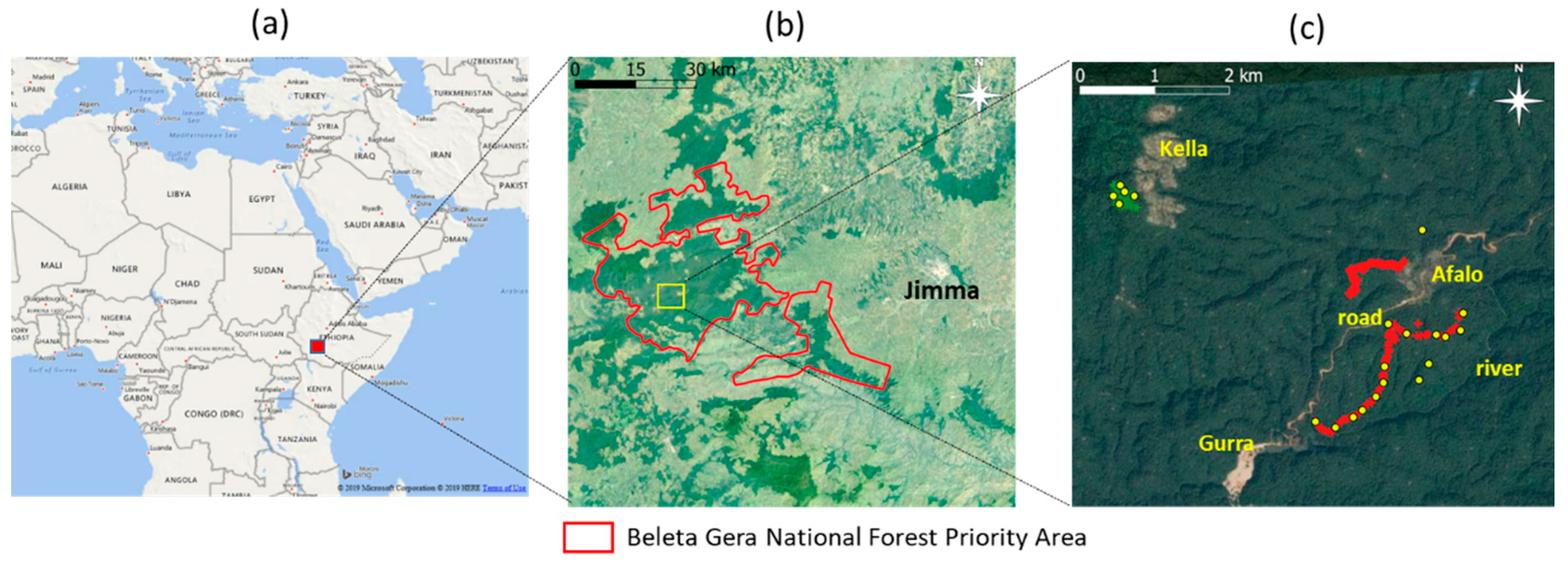
The area of this study is within Gera forest, southwest Ethiopia (Figure 1). Gera forest is part of the larger Belete-Gera National Forest Priority area, which occupies around 150,000 ha in Jimma zone and is located approximately 50 km to the west of Jimma town (Figure 1). The Belete-Gera forest consists of undulating hills in the 1500–2500 m range with steep mountainous terrain in some places. Coffee planting in Gera forest probably goes back more than two centuries, although originally on a restricted scale [11]. Over the past decades, large areas of natural forest have been transformed through the transplanting of seedlings from stands of wild coffee deep in the forest to create extensive forest coffee areas nearer to villages. Some farmers live near the coffee forest and regularly visit and manage their coffee forest. Some of the coffee forest is less managed as the farmers live at some distance away and come only for the harvesting season. Major areas of natural forest in the high altitude (over 2000 m) are not managed by the farmers for coffee production as it too cold for coffee production. However current climate changes suggest that the optimal altitude for coffee production is increasing [27].
In this research, two types of forest were studied. The undisturbed natural forest (NF) and heavily managed coffee forest (HMCF). NF is typically defined as a forest area which has seedlings, saplings, lianas, high biomass, and large number of trees with closed tree canopy. HMCF is a forest area that is frequently visited by the farmers for coffee production, and most of saplings, seedlings, and lianas have been removed. In this type of coffee forest, tree shade is considerably reduced by selective or unselective felling to facilitate effective coffee production.
We conducted in-situ field surveys during a dry season between 19 and 25 February 2019 (Table 1). The NF survey site is located near a remote settlement (Kella) in a high mountain region (above 2000 m) (marked as green crosses near village Kella in Figure 1c). The HMCF survey sites include the areas to the west of a small village called Afalo and to the south of Afalo (between the village and river) (red dots in Figure 1c).
2.1.2. Canopy Cover Photography
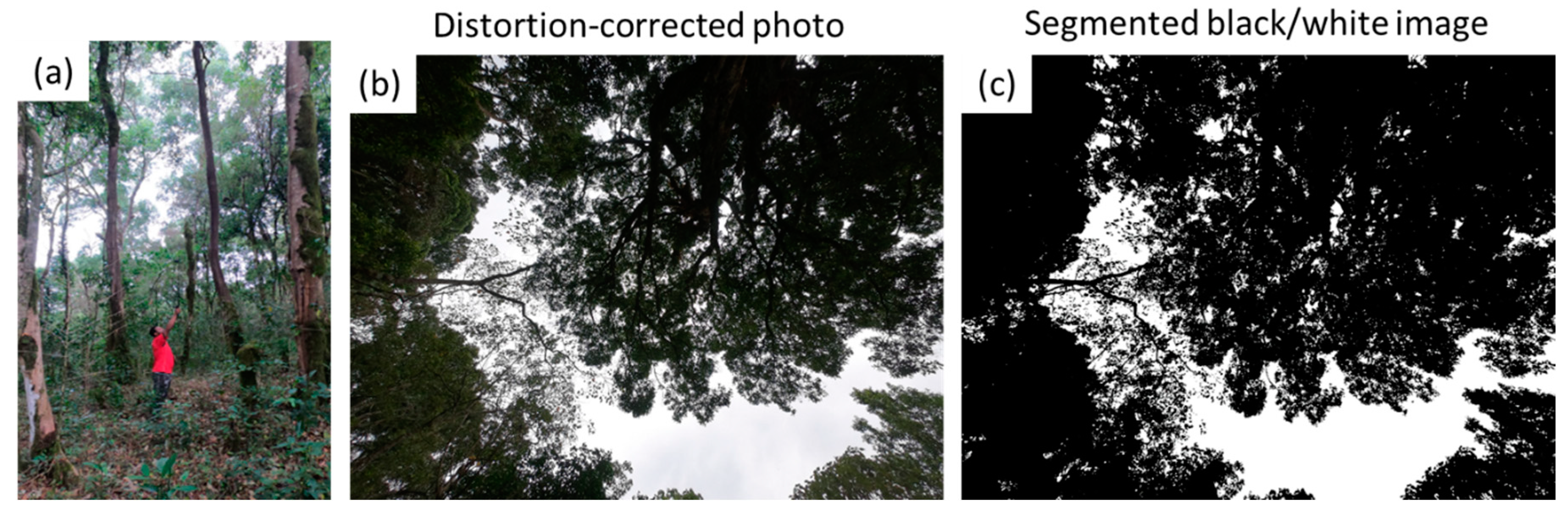
The ground truth fieldwork consisted of canopy cover photography, tree biodiversity survey, and general site description. The canopy cover photography was taken by using GoPro® Hero7 Black camera (wide angle) attached to a 1-m expandable camera pole (Figure 2a), so the canopy photos were taken about 2 m above the ground. Photos were taken every 10–20 steps along the transects. During the photo taking, we tried to keep the height of the camera at ≈2 m above the ground and the level of the pole consistent by holding it as straight as possible. To capture the natural canopy condition of the forest, the canopy photos were taken while we randomly diverted at least 10 m from the pathway (track) into the forest. To derive the canopy fraction from the photos, GPS coordinates of each photo were first extracted, and the photos were then corrected for wide-angle distortion following MATLAB® Fisheye calibration procedure. All distortion-corrected photos were then segmented into black (canopy) and white (sky) image using the Kernel Graph Cuts (KGC) algorithm [28,29]. The KGC can handle the light variation within the image well to delineate accurate canopy cover (black area in Figure 2b,c). However, some photos were contaminated by direct sun light, and these images were identified and removed from the analysis. To avoid the oversampling of canopy photos, we selected the photos that are at least 10 m apart. The canopy cover fraction was calculated from the segmented canopy cover image (note: canopy cover includes tree branches and stems).
2.1.3. Tree Biodiversity Survey
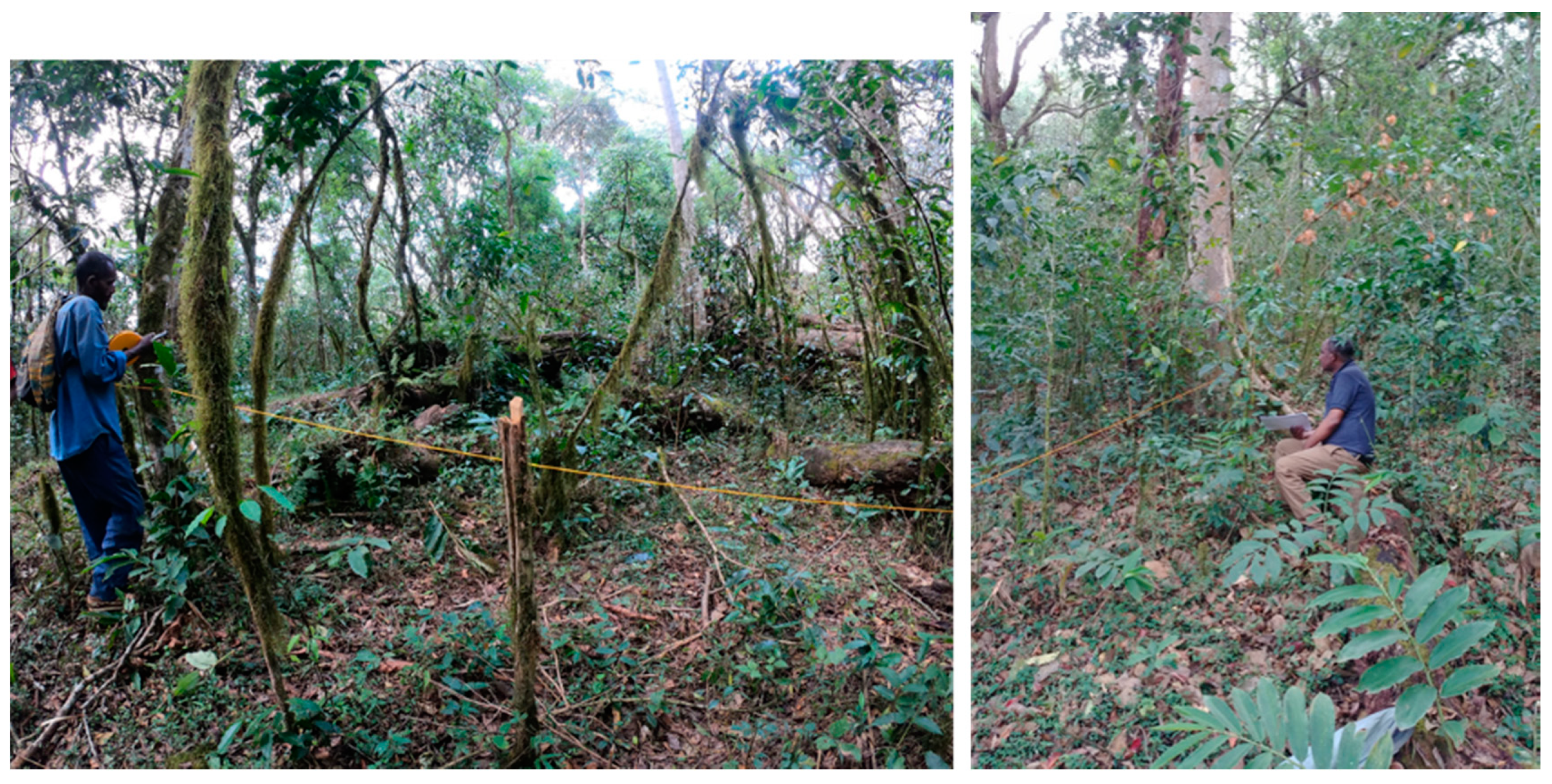
Tree diversity surveys were conducted in the two forest categories following the same transect line used for the photography. On each transect, plots of 20 × 20 m were laid at a distance of 200 m from each other. In each plot, trees of more than 5 cm diameter at breast height (DBH) were identified and recorded (Figure 3). The basal area was calculated from DBH and expressed in hectares. We recorded the GPS coordinates and altitude of each plot. A total of 21 sites were surveyed for both forest types during the dry season: five sites at the NF area and 16 sites at the HMCF area. We also recorded tree heights, and described disturbance at the tree survey sites. Species similarity between NF and HMCF sites was estimated using Sorenson’s similarity coefficient [30]
where, Ss is Sorensen’s similarity coefficient; a is number of species shared by the two forests; b is the number of species in NF; c is the number of species in HMCF.
2.2. Satellite Data and Processing
The list of satellite imagery used in this study is shown in Table 2. It includes 11 Landsat-5 (L5) Thematic Mapper (TM) and seven Landsat-8 (L8) Operational Land Imager (OLI) data (Table 2). Landsat data used in this study are Level 2 surface reflectance products (LEDAPS product for L5 TM and LaSRC product for L8 OLI), acquired from Earth Explorer at the U. S. Geological Survey (USGS). We only selected the data acquired in January and February. The 2019 image (L8 OLI 20190130) were taken around 3 weeks before the field surveys (Table 1), and it was used for direct comparison with the ground-truth data, while other Landsat data were used for time-series analysis. The surface reflectance values were then used to calculate VIs as described below. Both L5 TM and L8 OLI images have the same spatial resolution at 30 m, yet there are some differences in spectral resolution for the bands between the two sensors. However, these differences are less evident for surface reflectance and associated vegetation indices [31].
In this research, we used two vegetation indices (NDVI and NBR). NDVI (Equation (2)) is a normalized ratio of near-infrared (NIR) and red surface reflectance, defined as [23]
Here, Rnir and Rred are surface reflectance in NIR (L5 TM band 4 and L8 OLI band 5) and red (L5 TM band 3 and L8 OLI band 4) wavelengths. NBR (Equation (3)) is a normalized ratio of NIR and SWIR reflectance, defined as [17]
Here Rswir is reflectance in SWIR (L5 TM band 7 and L8 OLI band 7).
2.3. Constructing Mean Composite Maps
To construct mean composite maps of NDVI and NBR, we first applied a median filter (3 × 3 pixels) to individual images and selected the pixels with clear and low probability of cloud (i.e., Landsat-5 pixel_qa = 66; Landsat-8 pixel_qa = 322), and calculated mean values for individual pixels for the period of interest.
2.4. Tie-Point Approach
Tie-point methods have been used in various remote sensing fields [32,33,34]. “Tie-points” defines typical states of certain surface types. For land cover application, Asner and Lobell [32] used tie-points to define surface-type specific spectral endmembers for spectral unmixing algorithm to automatically identify dominant land types (green vegetation, litter, and bare soil) from the Airborne Visible and Infrared Imaging Spectrometer data. In estimating the concentration of sea ice in the Arctic, a tie-point can be assigned to passive microwave signature values typical of 100% ice concentration (tie-point for ice) and the other tie-point with values typical to open water (ice concentration = 0%, tie-point for water). The ice concentration can then be estimated from the relative distance between the two tie-points, e.g., ice concentration is estimated at 50% if the observed value lies halfway between the two tie-points [33].
In this study, we adopted this concept to estimate degradation (Im) caused by intensive management practices in the coffee forest. The proposed algorithm utilizes the tie-points in the NDVI and NBR domains. The tie-points characterize the typical states for undisturbed natural forest (NF) and heavily managed coffee forest (HMCF). With known tie-points for NF and HMCF, satellite-derived NDVI (Equation (4)) and NBR (Equation (5)) can be expressed as:
where, NDVINF and NDVIHMCF are the NDVI tie-points for NF and HMCF, respectively, and NBRNF and NBRHMCF are the NBR tie-points for NF and HMCF, respectively. Indvi and Inbr are the intensity of management for NDVI and NBR respectively, ranging between 0 and 1. Equations (4) and (5) can be rearranged in terms of Indvi (Equation (6)) and Inbr (Equation (7)) as:
NDVI and NBR may a different sensitivity in identifying the level of intensive management. In this proposed method, we consider the intensity of management (Im) (Equation (8)) in coffee forest as a weighted sum of the intensity of management estimated from NDVI and NBR.
where, W is a weighting between NDVI and NBR and Im is the level of intensive management in coffee forest, ranging between 0 and 1. If Im is close to 1, the observed NDVI and NBR get close to NDVIHMCF and NBRHMCF, so the area is likely intensively managed. If Im is close to 0, the observed NDVI and NBR get close to NDVINF and NBRNF, so the area is likely in undisturbed natural forest. In the following sections, we use the equal weighting between NDVI and NBR, i.e., W = 0.5.
3. Results
3.1. Ground Truth Fieldwork Data
3.1.1. Canopy Cover Fraction
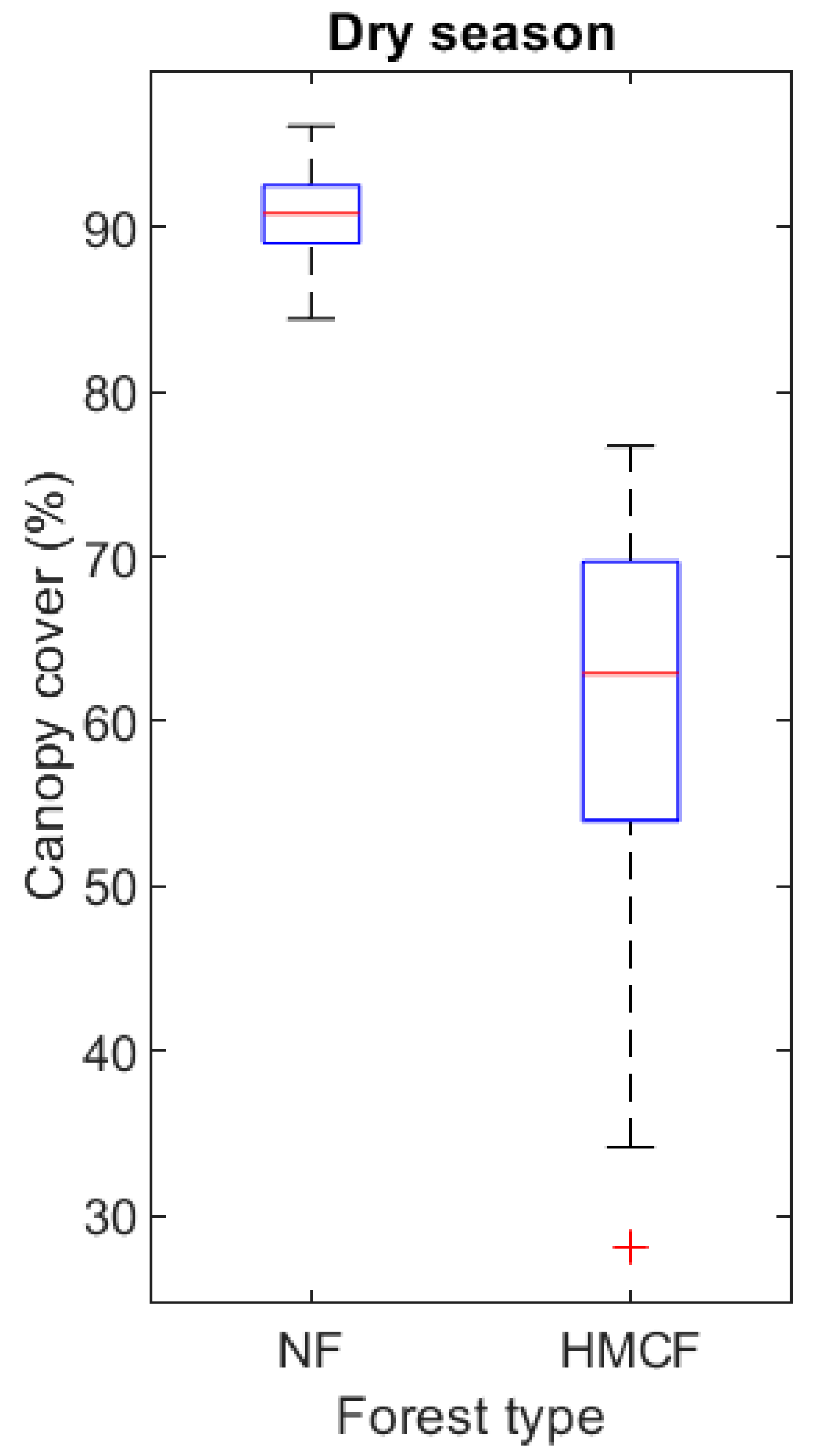
Figure 4 shows the results from tree canopy cover fraction (CF) derived from GoPro Hero7 camera photos acquired during the field surveys (Table 1). During the dry season, the mean CF value at the NF site is almost 91%, yet the mean CF value at the HMCF site reduces to 61% (Figure 4), which is almost 30% lower than the mean value at the NF site. The standard deviation (SD) of CF at the HMCF site is 10%, and this is much higher than the one at the NF site (3%). This indicates more diverse canopy conditions at the HMCF site. The separation in CF between NF and HMCF is statistically significant with 99% confidence (Welch’s t-test, p-value < 0.01), indicating that there is a distinctive difference in canopy cover during the dry season between undisturbed natural forest and heavily managed coffee forest.
3.1.2. Tree Biodiversity Survey
Table 3 contains the mean and SD values of tree biodiversity parameters collected from the tree surveys in NF and HMCF. The number of tree species (>5 cm in DBH) in the NF area is slightly higher than the number of the species in the HMCF area (not statistically significant, Welch’s t-test, p-value = 0.34). On the other hand, the number of trees in the NF area is significantly higher than the HMCF area with 95% confidence (Welch’s t-test, p-value = 0.03) (Table 3). For example, the number of trees (>5 cm in DBH) is almost 36 in the NF, while only 15 trees in the HMCF area. The basal area in the NF area is much larger than in the HMCF area (statistically significant with 99% confidence, Welch’s t-test, p-value < 0.01). It is a common practice that the farmers in Gera do not target specific canopy tree species either to remove from or to retain in the managed coffee forest, so we observe similar types of the tree species between NF and HMCF. However, the selective cutting of canopy trees results in significantly fewer canopy trees in the intensively managed coffee forest areas.
The results from Sorenson’s similarity coefficient (Ss) (Equation (1)) shows that the overall similarity between NF and HMCF sites is about 70%. In NF, most of the tree species are evergreen trees with some pockets of deciduous tree species. On the other hand, HMCF are dominated with deciduous species such as Albizia gummifera and Millettia ferruginea, due to the selective removal of broad-leaved evergreen trees by the farmers during their selective management and retention of species.
3.2. Satellite Data Analysis for the 2019 Imagery
3.2.1. Spectral Characteristics
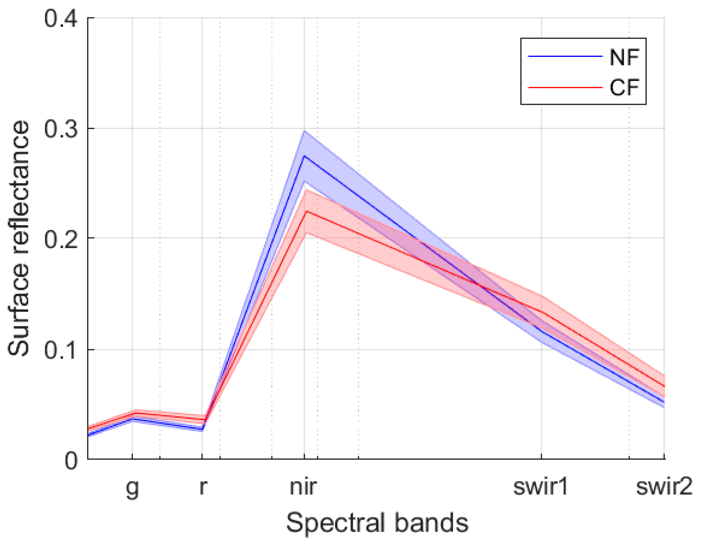
The spectral reflectance from the 2019 L8 OLI imagery shows distinctive characteristics between NF and HMCF. At the red bands, the mean reflectance value at the NF site is consistently lower by 0.01 than the values at the HMCF site (Figure 5). At NIR, the mean reflectance value at the NF site is almost 0.05 higher than the mean value at the HMCF site. The reflectance from both NF and HMCF sites decreases at the SWIR bands, yet the NF reflectance value further decreases by 0.02, compared to the HMCF reflectance value. These spectral characteristics are as expected because we observed less canopy cover (Figure 4) and more disturbance (e.g., slashing of saplings and seedlings) at the HMCF site.
3.2.2. Vegetation Indices
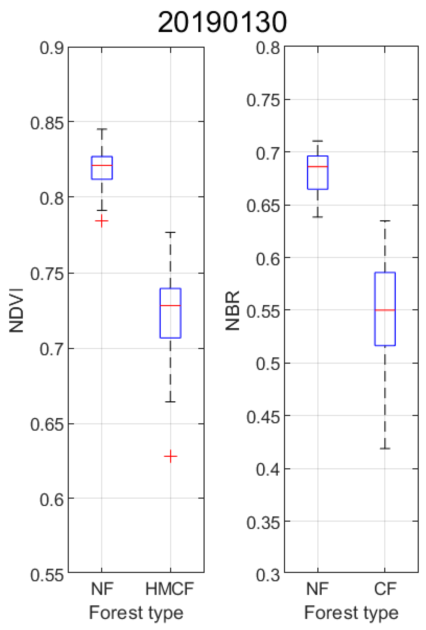
Figure 6 summarizes the difference in NDVI and NBR between the NF and HMCF sites, which is derived from the 2019 L8 OLI imagery. Similar to what we found in the spectral reflectance response (Figure 5), both NDVI and NBR show a clear distinction between NF and HMCF. The mean NF NDVI value is almost 0.137 higher than the mean HMCF NDVI value (Figure 6). Similarly, the mean NF NBR value is 0.178 higher than the mean HMCF NBR value (Figure 6). The NDVI and NBR values are significantly different with 99% confidence (Welch’s t-test, p-value < 0.01). Note that both NDVI and NBR values at the HMCF site have higher SD values than the ones at the NF site. A similar pattern can be seen in canopy cover fraction (Figure 5), in which the SD of canopy cover at the HMCF site is almost three times larger.
3.2.3. Comparison between Vegetation Indices and Canopy Cover
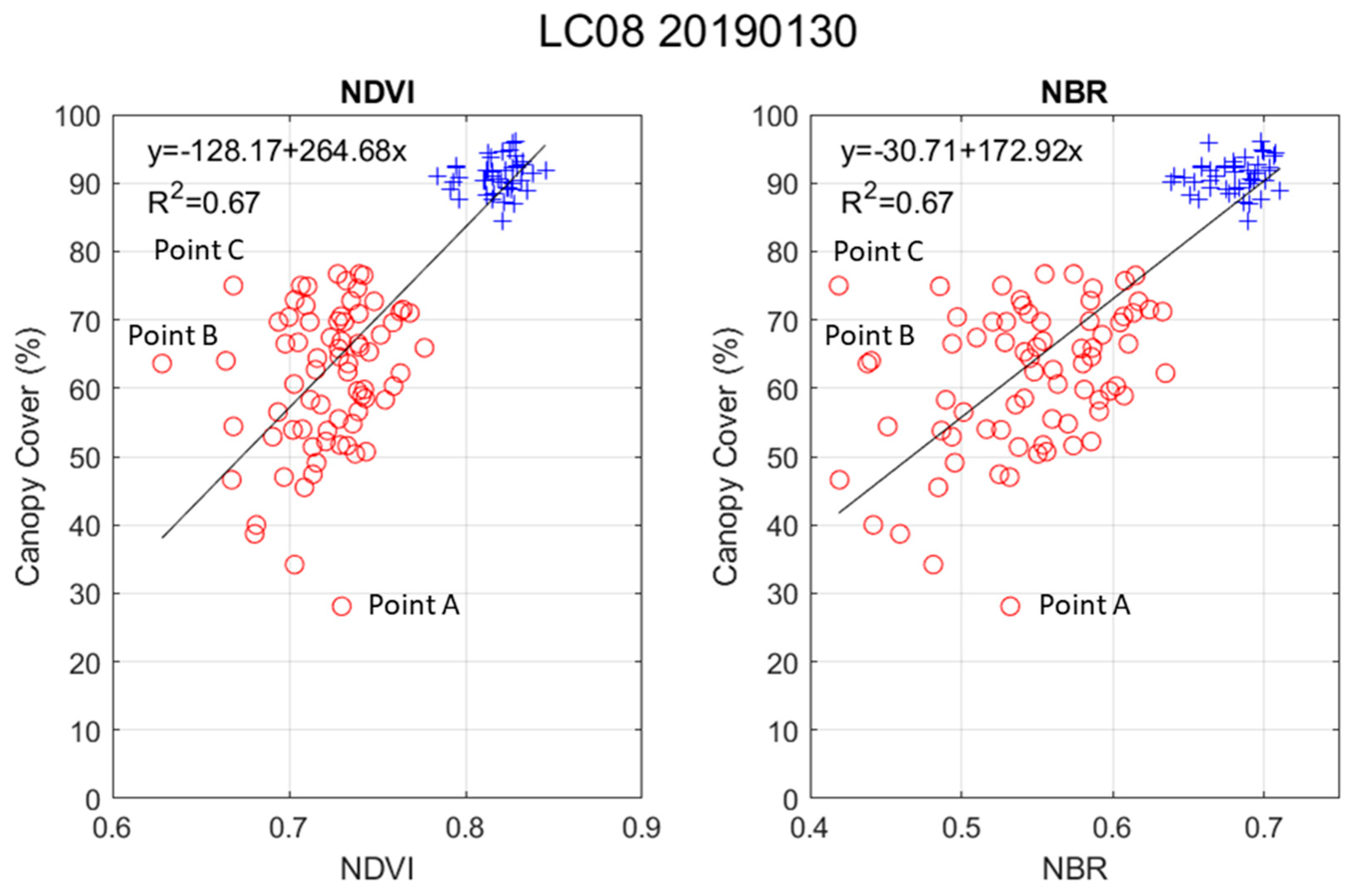
Now we compare NDVI and NBR with the in-situ canopy cover fraction from the 2019 survey. Note there is 19–26 days of difference in dates between the canopy surveys and the 2019 L8 OLI imagery (Table 1 and Table 2). Although changes in the canopy cover may occur within 26 days, we consider both the L8 OLI imagery and the in-situ canopy cover represent the dry-season condition in 2019. Regression analysis shows a positive association between NDVI (or NBR) and the in-situ canopy cover fraction (CF). The regression analysis shows that 67% of the variance in NDVI or NBR is explained by the canopy cover variance (R2 = 0.67) (Figure 7).
3.3. Temporal Evolution of NDVI and NBR between NF and HMCF
Results from previous sections suggest that the canopy cover, NDVI, and NBR from heavily managed coffee forest (HMCF) are significantly different from those from undisturbed natural forest (NF). The results also indicate that the reduced canopy cover in HMCF (due to felling of trees) is a major factor for there being distinctive differences in NDVI and NBR between NF and HMCF. In this section, we investigate how NDVI and NBR values from NF and HMCF have changed during the past 32 years. For this, we analyzed 17 Landsat imagery from 1987 to 2019 (Table 2). For the analysis, we used the pixels with clear or a low presence of cloud. However, variable atmospheric aerosol and moisture conditions may affect the retrieval of surface reflectance, although vegetation indices reduce such atmospheric influence.
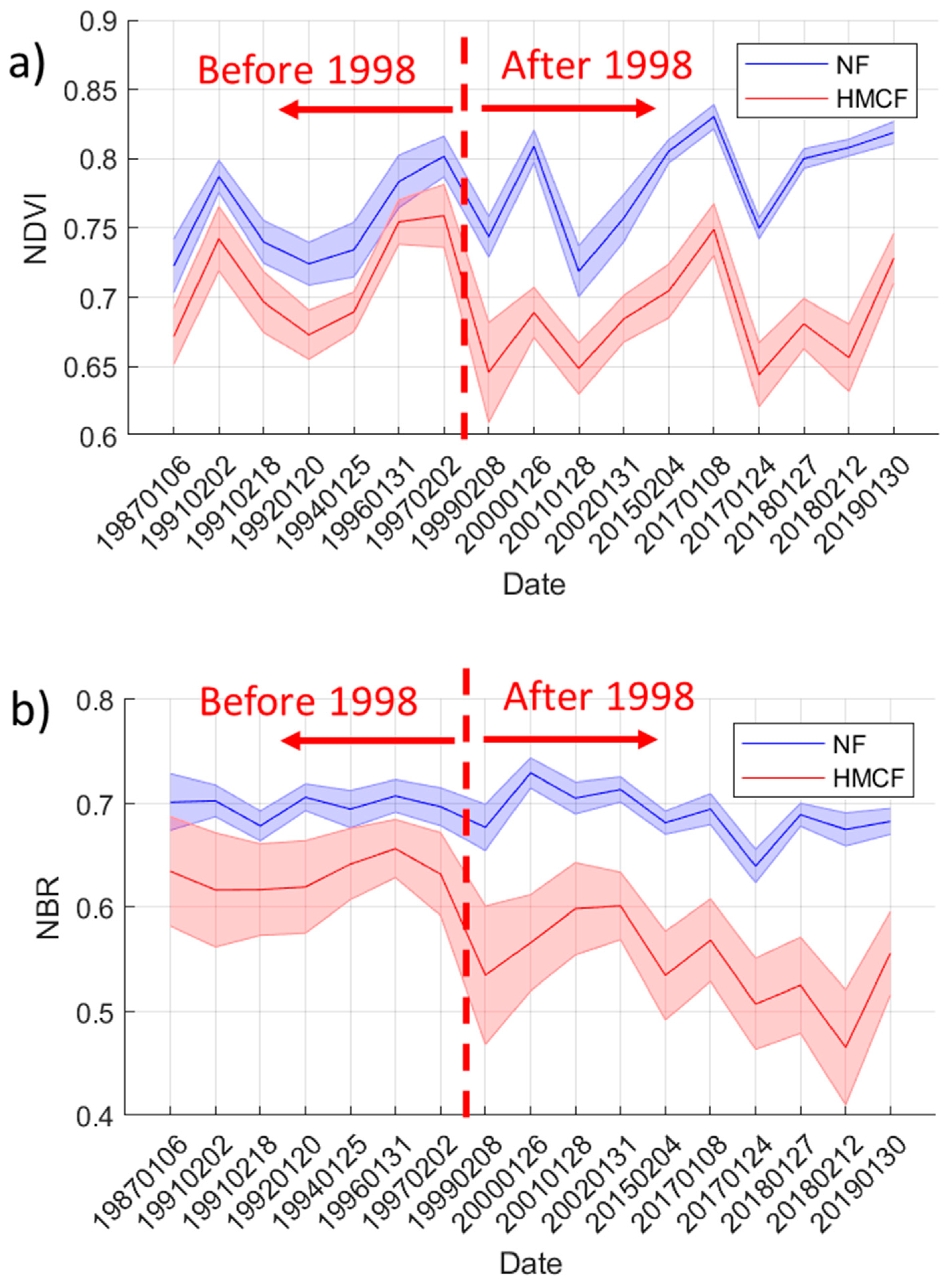
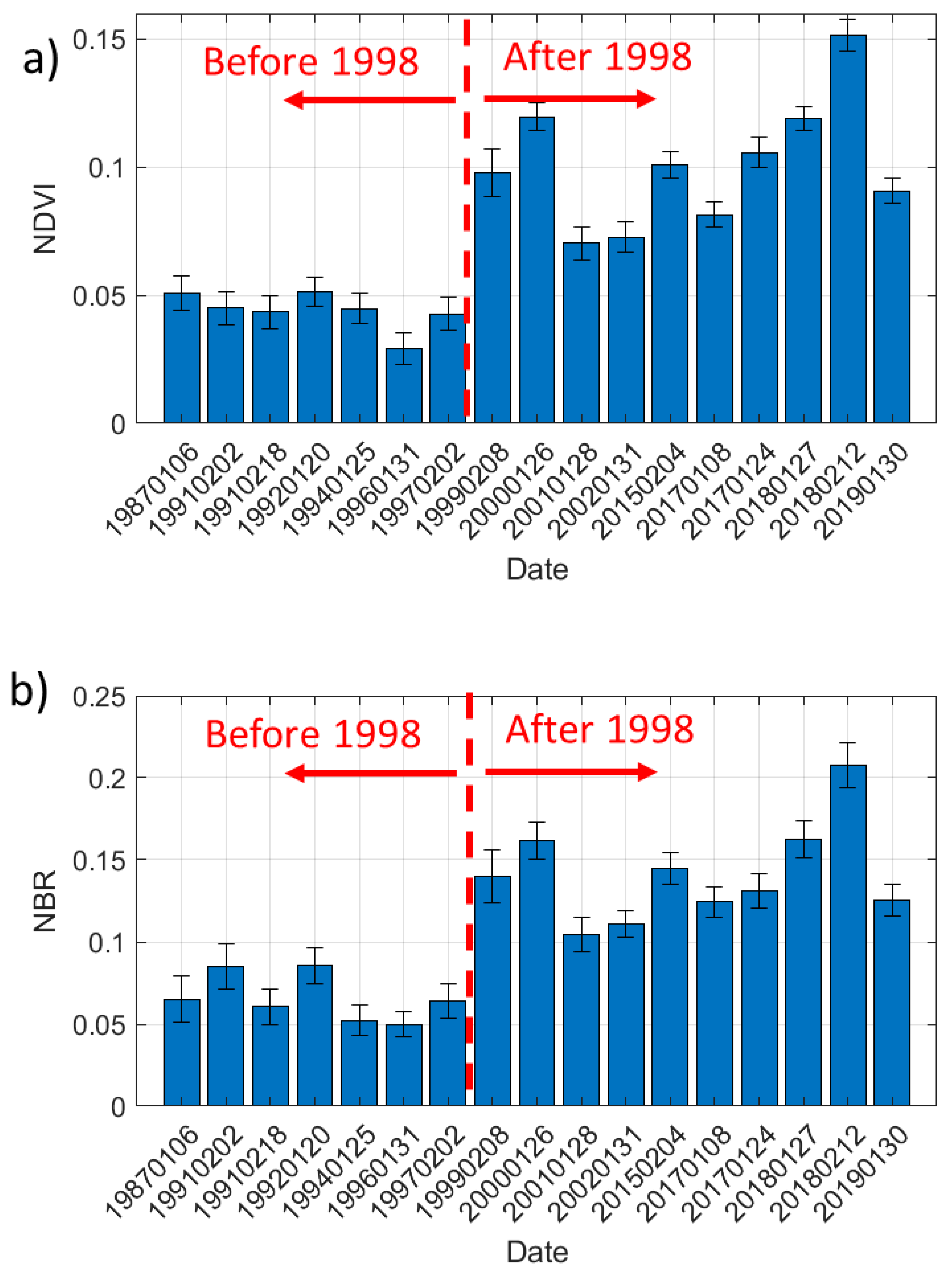
Figure 8 shows the temporal evolution of NDVI and NBR between 1987 and 2019. The results from the time-series analysis show that both NF and HMCF vegetation indices vary from image to image (Figure 8). The mean NDVI values at the NF site vary by 0.11, and the range of difference in NDVI is 0.10 at the HMCF site (Figure 8a). Therefore, the range of difference in NDVI is comparable between the NF and HMCF sites. However, the range of difference for NBR is not comparable between the NF and HMCF sites. For instance, the range of difference in NBR at the NF site is 0.09, but the range difference in NBR at the HMCF site is 0.22, which is almost twice the range for the NF site (Figure 8b).
It is worth noting that NDVI and NBR at the NF and HMCF sites fluctuates similarly, although NBR shows less obvious synchronous fluctuation (Figure 8a). This suggests that, despite the year-to-year variation in NDVI and NBR, the distance between the two means of NF (blue line) and HMCF (red line) stays consistently apart each other (Figure 8). In Figure 9, the relative separation in NDVI and NBR between NF and HMCF is plotted. Here it should be noted that the NF-HMCF NDVI separation remains below 0.06 until 1997. After that date the separation remains consistently larger. The NF-HMCF NBR separation also exhibits a similar trend. This result suggests that the relative separation in NDVI and NBR between NF and HMCF can be used to identify the high level of management within HMCF, despite the year-to-year variation due to variable atmospheric and vegetation conditions.
3.4. Estimating Degradation Caused by Intensive Management Practices Using the Tie-Point Method
3.4.1. Comparison of Mean State of NDVI and NBR between Two Periods (1987–1997 vs. 1999–2019)
Results from previous sections show possibilities and challenges in identifying the areas of heavily managed coffee forest (HMCF). They show that the level of management in HMCF (i.e., selective cutting, slashing of saplings and undergrowth, removing lianas, and sweeping the forest floor) affects canopy cover and other vegetation (Figure 4), and in turn affects NDVI and NBR within HMCF (Figure 5). The distinction between NF and HMCF caused by the intensive management practice is very clear with a high level of statistical significance. Despite this clear distinction, the time-series analysis shows that NDVI and NBR change from image to image due to variable atmospheric and vegetation conditions (Figure 8). This makes it difficult to identify the intensity of management in the coffee forest consistently throughout the years. The relative separation in NDVI and NBR between NF and HMCF, however, has consistently remained is relatively the same within the two periods (Figure 9).
The temporal variations in the relative separation in NDVI and NBR exhibits a clear distinction between two periods (1987–1997 and 1999–2019) with 99% confidence (Welch’s t test, p-value < 0.01). The relative separations of NDVI and NBR are, on average, 0.04 (±0.007) and 0.07 (±0.014), respectively, for the period of 1987–1997, and the corresponding separations increase to 0.10 (±0.025) and 0.14 (±0.030) for the period of 1999–2019 (Figure 9), almost more than two times higher than the 1987–1998 period. This result indicates that two distinctive periods exist before and after 1998. Both NDVI and NBR composite maps highlight an expansion of intensification of HMCF near the villages Afalo and Gurra, yet very little changes near the village Kella on the mountain. The NBR maps also show similar intensification near the village Afalo and also in pockets of areas in the south near the village Gurra (Figure 10).
3.4.2. Estimating the Intensity of Management Using Mean Tie-Points
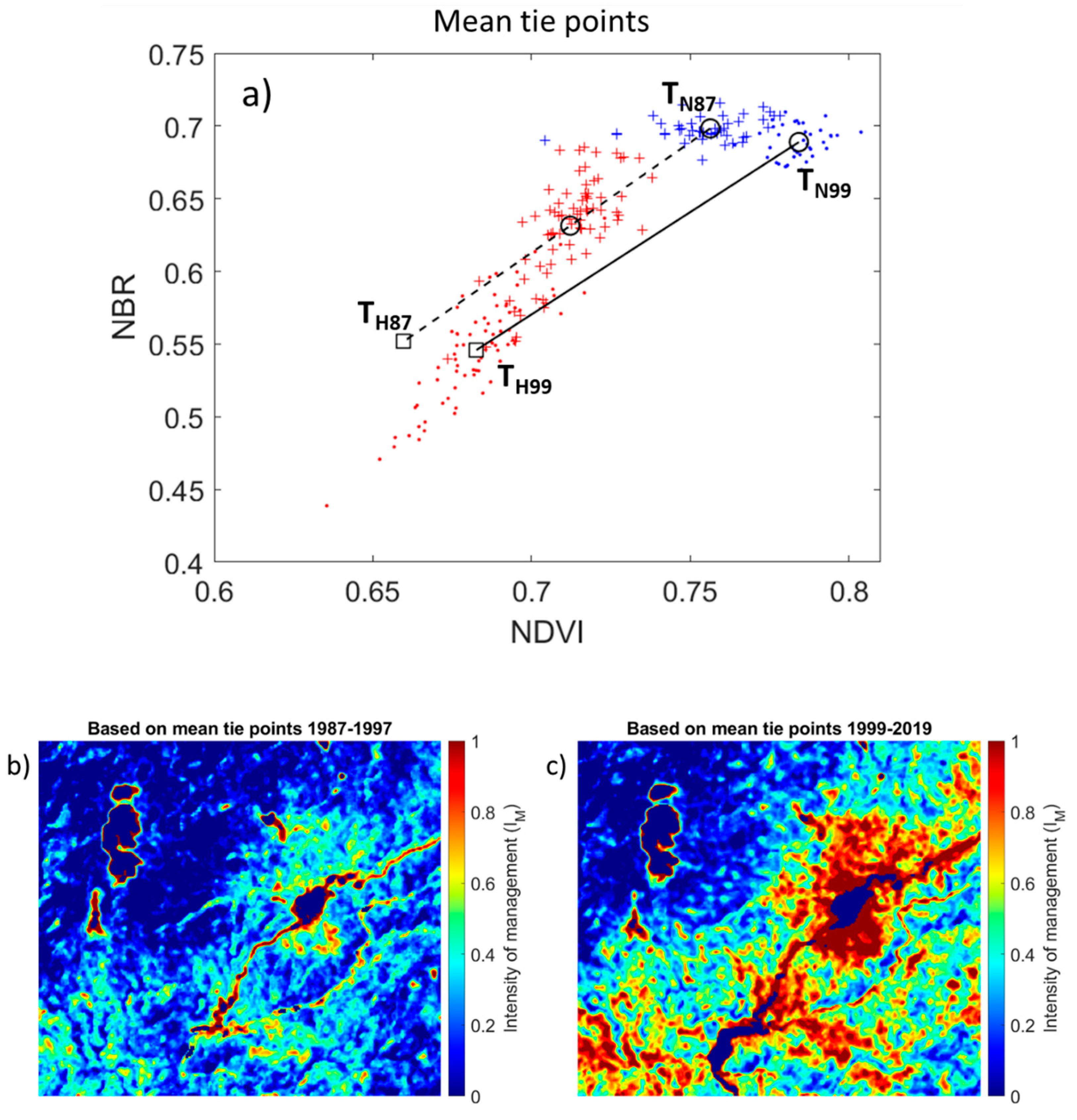
For a consistent estimation of the intensity of management between the two periods (1987–1997 and 1999–2019), it is important that the tie-points are selected at the same scale so that the estimated intensity can be compared between the two periods. For this purpose, we used the 1999–2019 period as a reference to estimate the change from the 1987–1997 period. As a first attempt, we consider the mean values as tie-points. The mean values at the NF and HMCF sites from the 1999–2019 composite map are shown as open circle and square, respectively, in Figure 11a, and these mean values were selected as the tie-points for NF (TN) and HMCF (TH). For the 1987–1997 period, the mean NF value was also selected as the tie-point for NF (TN87), as a typical state of undisturbed forest for that period. Note that the mean NF values are different between the two periods. The 1987–1997 NF mean value shifts to a lower NDVI, compared to the 1999–2019 value (Figure 11a).
It is worth noting that the distance in mean values between NF and HMCF for the 1987–1997 period is shorter than the one for the 1999–2019 period (Figure 11a). The 1987–1997 mean HMCF value is shown in an open circle on the dotted line connecting between TN87 and TH87 in Figure 11a. The distance between the two mean values is 0.0801 for the 1987–1997 period, which is 0.0978 shorter than the distance for the 1999–2019 period (Figure 11a). In Section 3.3, we found the relative distances in NDVI and NBR between NF and HMCF were different for the two periods but consistent within each period. The shorter distance between NF and HMCF for the 1987–1997 period indicates the level of management was low in coffee forest. To compare the intensity of management (degradation) between the two periods, we extended the distance between TN and TH for the 1987–1997 period to match the distance (=0.1779) between TN87 and TH87 for the 1999–2019 period, so that the estimated Im can be compared at the same scale for both periods.
The derived results reveal a progressive but significant change in the intensity of management between the two periods (Figure 11b,c). During the 1999–2019 period, the expansion and intensification of management are clearly seen near the villages Afalo and Gurra (Figure 11c). It should be noted that, as the tie-point for HMCF (TH99) was selected based on the means from the 1999–2019 composite, the intensity of management is likely overestimated. For example, the HMCF data points for the 1999–2019 period spread around TH99, and some data points have NDVI and NBR values much lower than TH99, so passing beyond TH99 (Figure 11a). In other words, the maximum intensity of management was tied to an intermediate level of intensity, so causing overestimation. In the next section, we will adjust TH to a lower NDVI and NBR to better represent the maximum intensity of management.
3.4.3. Estimating the Intensity of Management Using Adjusted Tie-Points
For the adjusted tie-points, we kept the tie-points for NF (TN) the same, but adjusted the tie-points for HMCF (TH) to better represent the maximum intensity of management. To do this, we selected one of the HMCF data points from the 1999–2019 composite map, located near the minimum NDVI and NBR, as TH99a (Figure 12a). We adjusted TH87a for the 1987–1997 period to match with new TH99a for the 1999–2019 period. The results are shown in Figure 12b,c. As the maximum intensity is scaled to a higher level of degradation, the intensive management is much less evident for the 1987–1997 period, when compared to the results with the mean tie-points. The new intensity maps show the expansion and intensification of management similar to the results from mean tie-points, yet a more realistic representation of the transition of intensive management across 1998. The results indicate that a certain level of degradation occurred near the villages Afalo and Gurra even during 1987–1997, but the level of intensive management was much lower (less than 50%) compared to the level of management during the period 1999–2019. This suggests a change in the way of managing coffee forest may have occurred at a regional or national scale in the mid-1990s.
4. Discussion
4.1. Can We Distinguish Heavily Managed Coffee Forest Areas from Undisturbed Natural Forest?
The results show that heavily managed coffee forest areas (HMCF) have distinctively less (almost 30% less) canopy cover than natural forest areas (Figure 4), and the basal area per hectare (>5 cm in DBH) is also significantly less in HMCF than in natural forest NF (Table 3). This suggests that canopy trees are regularly removed in the heavily managed coffee forest areas, especially broad-leaved evergreen trees, which reduces the aerial canopy cover in HMCF. This difference in canopy cover is evident in Landsat imagery as shown by the distinctively lower NDVI and NBR in HMCF than in NF (Figure 6).
The direct comparison between vegetation indices and in-situ canopy cover fraction indicates that both NDVI and NBR are strongly influenced by the reduced canopy cover in HMCF (R2 = 0.67) (Figure 7). The remaining unexplained variance can be attributed to changes in other aspects of forest structure (e.g., slashing of saplings and seedlings and removal of lianas), difference in spatial and temporal resolution between the L8 OLI imagery and in-situ survey, and atmospheric influence. Particularly large variance in the regression analysis occurs in the HMCF points (Figure 7). The outliers are mainly attributed to sub-pixel variability of canopy cover. For instance, in Figure 7 outliers marked as A, B, and C demonstrate such sub-pixel variability. The canopy cover observed at Point A is only 28.1% as the photo was taken in a very open area, although we observed a more closed canopy just 10 m away from that point. On the other hand, Point B in Figure 7 shows the opposite case. At this location, the canopy photo taken has a more closed canopy (63.6%), yet we observed open areas adjacent to that point. At Point C, the canopy cover derived from canopy photo is 75%, while NDVI and NBR are low. At this point, the canopy photo contains low-level canopies from tree saplings, which cause a bias in estimating canopy cover from the photo. Apart from this sub-pixel variability, 67% of the variance in canopy cover can be explained by either NDVI or NBR (Figure 7).
The time-series analysis of vegetation indices shows that NDVI fluctuates much more than NBR (Figure 8). This fluctuation is likely to be due to the combined effects from variable atmospheric and vegetation conditions for the individual images. Previous research reports that NDVI is sensitive to leaf area, i.e., red absorption by photosynthesis and higher NIR reflectance by leaves [24], while NBR is more sensitive to leaf water content in the forest, i.e., lower SWIR by moist vegetation and lower NIR reflectance by less leaf area [21]. Despite, the different sensitivity between the two indices, the regression analysis showed a similar explained variance for the reduced canopy cover (Figure 7). This suggests that the reduced canopy cover and consequent dryness in HMCF similarly affect both NDVI and NBR in 2019.
It is not certain why NDVI exhibits higher fluctuation than NBR. The use of the Enhanced Vegetation Index (EVI) [35] significantly reduces the range of the fluctuation, i.e., only ≈0.02–0.03 while 0.11 for NDVI, but the synchronous fluctuation feature shown in NDVI disappears. Using EVI in mountainous regions is not recommended as it is more sensitive to topographic effects than NDVI [35]. However, this tells us that larger, synchronous fluctuation in NDVI is likely to be affected by image-to-image variations in atmospheric conditions. Another factor which may explain the larger fluctuation in NDVI is phenological variations due to variable rainfall each year. The forest in the study area is typically considered as evergreen. However, both NF and HMCF still contain a portion of deciduous trees (≈3% in NF and ≈27% in HMCF of the total trees) and undergoes phenological changes each year. Variable rainfall changes the timing of shedding and may also be a factor. As NDVI is more sensitive to leaf area ([24]), such phenological changes may affect NDVI. Despite the fluctuations, the relative separation in either NDVI or NBR between NF and HMCF shows a consistent pattern (Figure 9). Assuming atmospheric and phenological conditions are the same in each image, this relative separation estimated from each image would reduce any image-to-image variations caused by atmospheric and phenological changes. Nonetheless, our results show that intensively managed coffee forest areas can be clearly distinguished from the natural forests in terms of canopy cover, biodiversity, and vegetation indices.
4.2. Can We Consistently Quantify the Level of Degradation Caused by Intensive Management in the Coffee Forest?
The results from in-situ observations and time-series analysis of Landsat imagery show a way that the relative separation in NDVI or NBR between NF and HMCF can be used to estimate degradation caused by intensive management practices in a consistent way. One should note that the relative separation in both NDVI and NBR has increased significantly after 1998 (Figure 9). To minimize the effects from any seasonal variation, we only selected Landsat imagery that was acquired during the peak of dry season, i.e., January and February (Table 2). However, phenological changes can vary each year or even during the dry season due to variable weather conditions, which affects the relative separation derived from the individual images. These image-to-image variations in the relative separation are relatively small, compared to the means from two distinctive periods (1987–1997 and 1999–2019) (Figure 9). For NDVI, the mean and SD values are 0.044 ± 0.003 and 0.101 ± 0.007, respectively, for the 1987–1997 and 1999–2019 periods. For NBR, the mean and SD values are 0.066 ± 0.005 and 0.141 ± 0.009, respectively, for the 1987–1997 and 1999–2019 periods. In both cases, the relative separations between the two periods are statistically different with 99% confidence (Welch’s t-test, p-value < 0.01). This suggests that changes in degradation can be estimated between the two periods if a proper measurement scale can be found.
Figure 11 and Figure 12 show that a tie-point approach can be used to estimate the long-term changes in degradation caused by intensive management practices. In this approach, we fixed tie-points for NF to the mean and standard deviation values for the two periods, which is 0.756 ± 0.013 and 0.698 ± 0.008, respectively, for NDVI and NBR for the 1987–1997 period, and 0.784 ± 0.007 and 0.689 ± 0.011 for the 1999–2019 period. The combined standard deviations of NDVI and NBR for NF are 0.011 and 0.010 for the two periods. For the adjusted tie-point approach, this contributes to the errors of ≈4.2% in estimating the intensity of degradation in the coffee forest. The image-to-image variations in the relative separation in NDVI and NBR (Figure 9) can contribute to the errors in estimating the level of degradation. The standard deviations of the relative separation for NDVI and NBR are 0.007 and 0.014, respectively, for the 1987–1997 period, and 0.025 and 0.030 for the 1999–2019 period. The combined standard deviations are 0.011 and 0.028 for the two periods, which contribute to the errors of up to ≈10% in estimating the level of degradation.
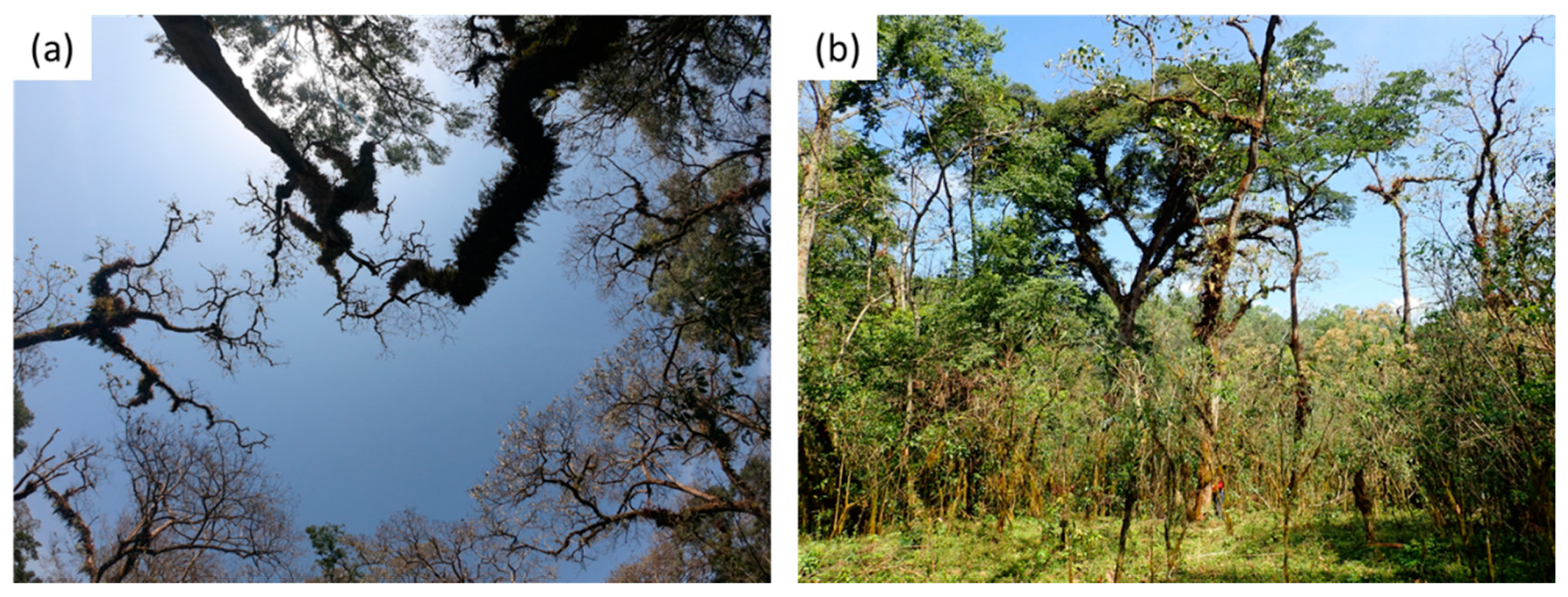
The estimation of degradation is also affected by the selection of tie-points for HMCF. For the adjusted tie-point method, we selected the tie-point in the area where most of canopy trees were removed (canopy cover = 38%) (Figure 13). The area is also characterized by clearing of saplings and undergrowth, as well as sweeping of the floor (leaving only dry grass on the ground) (Figure 13). It is important to note that the maximum degradation estimated by the adjusted tie-point method is tied to this particular condition as shown in Figure 13, i.e., IM = 1. It should be noted that selecting the tie-point for the maximum degradation may vary in different forest areas, depending on the level of management practices among different communities. However, as long as the tie-points can be properly selected and understood, our tie-point method can provide a way to assess the temporal changes in degradation caused by intensive management practices.
4.3. Understanding the Transition
The intensification of forest management which produces the major results in our data from 1998 onwards is the result of a combination of factors. In 1991 the military government was removed by the Ethiopian People’s Revolutionary Democratic Front (EPRDF) led movements. This involved the collapse of central government control for several weeks/months across the country during which time farmers took the opportunity to reassert their claims to particular areas of land, such as forest, from which they have been barred by the military regime [36]. As the new government asserted its control, it initially took a somewhat more relaxed view of forest use by farmers as there was pent up demand for farmland by young families and also interest in planting coffee seedlings in the forestland near to homesteads. Certainly, the new government was initially not so strict on forest protection as its military predecessor had been. However, with time while the liberal policies towards forest clearance did not continue, a positive attitude to coffee planting—either transplanting wild seedlings from within the natural forest or using nursery grown seedlings—was developed. This involved farmers in making a tax payment to the local government which allowed them “temporary” use of the government forest for forest friendly uses, such as coffee growing.
Once this arrangement became recognised in the areas suitable for coffee production there was a route through which farmers could respond to the 1994 and 1997 peaks in world coffee prices [37]. The sharp rise in coffee prices from lows in 1992/3 and 2001/2, and the way in this came through to the prices in country for the domestic coffee trade are also reported to be the cause of more intensive coffee forest management (Sutcliffe, Pers comm.). Ripe beans will fall to the floor, especially during harvesting or when disturbed by monkeys and other wild animals. As the value of this loss was recognized by “owners” of coffee forest, they required more intensive removal of the undergrowth and even sweeping away the ground cover so that their pickers would collect these berries and not leave them for other, poorer villagers to collect. Finally, from the early 1990s the European Union started a new phase in its support to Ethiopian coffee production. This included support to smallholders and to marketing systems which also encouraged the expansion and intensification of forest coffee production.
5. Conclusions
In addressing our research questions, distinguishing the intensively managed coffee forest areas from undisturbed natural forest areas using Landsat-derived vegetation indices (NDVI, NBR) is feasible with a high level of confidence. The intensive management practices in the coffee forest significantly reduce canopy cover, and the vegetation indices (NDVI, NBR) are strongly correlated to the reduced canopy cover.
The time-series analysis of 32 years of Landsat imagery (1987–2019) reveals a clear trend in the level of degradation caused by intensified management of the coffee forest, with the situation becoming markedly more severe from 1998 onwards. Our proposed tie-point method provides a way to estimate long-term changes in the degree of degradation in the intensively managed coffee forest, if proper tie-points can be selected. The results from the tie-point method suggests that the expansion of areas of intensive management of the coffee forest and the intensification of the consequent degradation of that forest occur in the study area, and this may follow the change of government in 1991 and the introduction of new economic policies, changed arrangements for access to government forest, as well as economic situation, i.e., rising coffee prices.
Future research is required to further validate the tie-point methods in different forest areas, along with co-located social and economic surveys to better understand the history and drivers of intensive management practice and tree biodiversity selection. Tree seed viability surveys are also needed to understand the impacts of such intensive management practices on forest regeneration. By putting these all together, the research can provide a scientific assessment of this hidden “degradation” within the coffee forest and inform the development of policies and practices for future coffee production in the forest which are ecologically sustainable and economically viable.
Author Contributions
Author contributions to this study are as follows: Conceptualization, B.H., K.H., A.W., B.M.; methodology, B.H., and K.H.; software, B.H.; validation, B.H., A.A., and B.M.; formal analysis, B.H., and K.H. investigation, all; resources, all; data curation, all; writing—original draft preparation, B.H., and K.H.; writing—review and editing, all; visualization, B.H.; supervision, B.H., K.H., and A.W.; project administration, B.H., and K.H.; funding acquisition, B.H. All authors have read and agreed to the published version of the manuscript.
Funding
This research was funded by University of Huddersfield.
Acknowledgments
The authors are grateful to Jimma University for collaborating in this project and to government staff in Gera who assisted in the fieldwork and contributed to the workshop at which initial findings were presented. Special gratitude to Afalo, Mohammed, Abba Sharo, Abba Dura, and Shabu Jemal in Gera for helping in the fieldwork. The Community Conservation of Wild Coffee and Natural Forest Management Project, run by the University of Huddersfield and the Ethio-Wetlands and Natural Resources Association from a base in Mizan Teferi, provided the initial field experience from which this project was developed and seconded staff to engage in the fieldwork.
Conflicts of Interest
The authors declare no conflict of interest.
References
- EFAP. Ethiopian Forestry Action Program; EFAP: Addis Ababa, Ethiopia, 1994. [Google Scholar]
- Eshetu, Z.; Högberg, P. Reconstruction of forest site history in Ethiopian Highlands based on 13C natural abundance of soils. AMBIO A J. Hum. Environ. 2000, 29, 83–89. [Google Scholar] [CrossRef]
- Reusing, M. Change detection of natural high forest in Ethiopia, using remote sensing and GIS techniques. Int. Arch. Photogramm. Remote Sens. 2000, 23, 1254–1258. [Google Scholar]
- WBISPP (Woody Biomass Inventory and Strategic Planning Project). Manual for Woody Biomass Inventory; Ministry of Agriculture: Addis Ababa, Ethiopia, 2000.
- FAO (UN Forest and Agriculture Organization). Forest Resource Assessment (FRA) for Ethiopia; FAO: Rome, Italy, 2010; Available online: http://www.fao.org/docrep/013/al501E/al501e.pdf (accessed on 26 November 2019).
- Anthony, F.; Combes, M.-C.; Astorga, C.; Bertrand, B.; Graziosi, G.; Lashermes, P. The origin of cultivated Coffee arabica L. varieties revealed by AFLP and SSR markers. Theor. Appl. Genet. 2002, 104, 894–900. [Google Scholar] [CrossRef] [PubMed]
- Gole, T.W. Vegetation of the Yayu Forest in SW Ethiopia: Impacts of Human Use and Implications for In Situ Conservation of Wild Coffea arabica L. Populations; Ecology and Development Series No. 10; Centre for Development Research, University of Bonn: Bonn, Germany, 2003. [Google Scholar]
- Senbeta, F. Biodiversity and Ecology of Afromontane Rainforests with Wild Coffea arabica L. Populations in Ethiopia; Ecology and Development Series No. 38; Cuvillier: Göttingen, Germany, 2006. [Google Scholar]
- World Bank. Ethiopia—Trade and Transformation: Diagnostic Trade Integration Study: Summary and Recommendations (English); World Bank: Washington, DC, USA, 2004; Available online: http://documents.worldbank.org/curated/en/479381468252005382/Summary-and-recommendations (accessed on 26 November 2019).
- Foreign Agricultural Service (FAS). Global Agricultural Information Network. In Ethiopia—Coffee Annual Report; GAIN Report 1904; USDA Foreign Agricultural Service: Washington, DC, USA, 2019. Available online: https://www.fas.usda.gov/data/ethiopia-coffee-annual-4 (accessed on 4 December 2019).
- Aregay, M. The early history of Ethiopia’s coffee trade and the rise of Shawa. J. Afr. Hist. 1988, 29, 19–25. [Google Scholar] [CrossRef]
- Wood, A.; Tolera, M.; Snell, M.; O’Hara, P.; Hailu, A. Community forest management (CFM) in south-west Ethiopia: Maintaining forests, biodiversity and carbon stocks to support wild coffee conservation. Glob. Environ. Chang. 2019, 59. [Google Scholar] [CrossRef]
- Aerts, R.; Hundera, K.; Berecha, G.; Gijbels, P.; Baeten, M.; Van Mechelen, M.; Hermy, M.; Muys, B.; Honnay, O. Semi-forest coffee cultivation and the conservation of Ethiopian Afromontane rainforest fragments. For. Ecol. Manag. 2011, 261, 1034–1041. [Google Scholar] [CrossRef] [Green Version]
- Hundera, K.; Aerts, R.; Fontaine, A.; Van Mechelen, M.; Gijbels, P.; Honnay, O.; Muys, B. Effects of coffee management intensity on composition, structure and regeneration of Ethiopian moist evergreen afromontane forests. Environ. Manag. 2013, 51, 801–809. [Google Scholar] [CrossRef]
- Sutcliffe, J.P. Personal communication. 2015. [Google Scholar]
- Lambert, J.; Denux, J.-P.; Verbesselt, J.; Balent, G.; Cheret, V. Detecting clear-cuts and decreases in forest vitality using MODIS NDVI time series. Remote Sens. 2015, 7, 3588–3612. [Google Scholar] [CrossRef] [Green Version]
- Key, C.H.; Benson, N.C. Landscape assessment: Ground measure of severity, the composite burn index; and remote sensing of severity, the normalized burn ratio. In FIREMON: Fire Effects Monitoring and Inventory System; General Technical Report RMRS-GTR-164-CD; Rocky Mountain Research Station; USDA Forest Service: Ogden, UT, USA, 2006. [Google Scholar]
- Hermosilla, T.; Wulder, M.A.; White, J.C.; Coops, N.C.; Hobart, G.W. Regional detection, characterization, and attribution of annual forest change from 1984 to 2012 using Landsat-derived time-series metrics. Remote Sens. Environ. 2015, 170, 121–132. [Google Scholar] [CrossRef]
- Jarron, L.R.; Hermosilla, T.; Coops, N.C.; Wulder, M.A.; White, J.C.; Hobart, G.W.; Leckie, D.G. Differentiation of alternate harvesting practices using annual time series of Landsat data. Forests 2016, 8, 15. [Google Scholar] [CrossRef] [Green Version]
- Tortini, R.; Mayer, A.L.; Hermosilla, T.; Coops, N.C.; Wulder, M.A. Using annual Landsat imagery to identify harvesting over a range of intensities for non-industrial family forests. Landsc. Urban Plan. 2019, 188, 143–150. [Google Scholar] [CrossRef]
- Keeley, J.E. Fire intensity, fire severity and burn severity: A brief review and suggested usage. Int. J. Wildland Fire 2009, 18, 116–126. [Google Scholar] [CrossRef]
- Liu, S.; Wei, X.; Li, D.; Lu, D. Examining forest disturbance and recovery in the subtropical forest region of Zhejiang province using Landsat time-series data. Remote Sens. 2017, 9, 479. [Google Scholar] [CrossRef] [Green Version]
- Tucker, C.J. Red and photographic infrared linear combinations for monitoring vegetation. Remote Sens. Environ. 1979, 8, 127–150. [Google Scholar] [CrossRef] [Green Version]
- Glenn, E.P.; Huete, A.R.; Nagler, P.L.; Nelson, S.G. Relationship between remotely-sensed vegetation indices, canopy attributes and plant physiological processes: What vegetation indices can and cannot tell us about the landscape. Sensors 2008, 8, 2136–2160. [Google Scholar] [CrossRef] [Green Version]
- Pettorelli, N.; Vik, J.O.; Mysterud, A.; Gaillard, J.M.; Tucker, C.J.; Stenseth, N.C. Using the satellite-derived NDVI to assess ecological responses to environmental change. Trends Ecol. Evol. 2005, 20, 503–510. [Google Scholar] [CrossRef]
- Sothe, C.; de Almeida, C.M.; Liesenberg, V.; Schimalski, M.B. Evaluating Sentinel-2 and Landsat-8 data to map sucessional forest stages in a subtropical forest in Southern Brazil. Remote Sens. 2017, 9, 838. [Google Scholar] [CrossRef] [Green Version]
- Moat, J.; Williams, J.; Baena, S.; Wilkinson, T. Resilience potential of the Ethiopian coffee sector under climate change. Nat. Plants 2017, 3, 17081. [Google Scholar] [CrossRef]
- Salah, M.B.; Mitiche, A.; Ayed, I.B. Multiregion image segmentation by parametric kernel graph cuts. IEEE Trans Image Process. 2011, 20, 545–557. [Google Scholar] [CrossRef]
- Hwang, B.; Ren, J.; McCormack, S.; Berry, C.; Ben Ayed, I.; Graber, H.C.; Aptoula, E. A practical algorithm for the retrieval of floe size distribution of Arctic sea ice from high-resolution satellite synthetic aperture radar imagery. Elem. Sci. Anth. 2017, 5, 38. [Google Scholar] [CrossRef] [Green Version]
- Kent, M.; Coker, P. Vegetation Description and Analysis: A Practical Approach; John Wiley and Sons, Inc.: Hoboken, NJ, USA, 1992. [Google Scholar]
- Flood, N. Counituity of reflectance data between Landsat-7 ETM+ and Landsat-8 OLI, for both top-of-atmosphere and surface reflectance: A study in the Australian landscape. Remote Sens. 2014, 6, 7952–7970. [Google Scholar] [CrossRef] [Green Version]
- Asner, G.P.; Lobell, D.B. A biogeophysical approach for automated SWIR unmixing of soils and vegetation. Remote Sens. Environ. 2000, 75, 99–122. [Google Scholar] [CrossRef]
- Cavalieri, D.J.; Gloersen, P.; Campbell, W.J. Determination of sea ice parameters with the Nimbus 7 SMMR. J. Geophys. Res. 1984, 89, 5355–5369. [Google Scholar] [CrossRef]
- Comiso, J.C.; Cavalieri, D.J.; Parkinson, C.L.; Gloersen, P. Passive microwave algorithms for sea ice concentration: A comparison of two techniques. Remote Sens. Environ. 1997, 60, 357–384. [Google Scholar] [CrossRef]
- Liu, H.Q.; Huete, A.R. A feedback based modification of the NDV I to minimize canopy background and atmospheric noise. IEEE Trans. Geosci. Remote Sens. 1995, 33, 457–465. [Google Scholar] [CrossRef]
- Ayana, A.; Arts, B.; Wiersum, K.F. Historical development of forest policy in Ethiopia: Trends of institutionalization and deinstitutionalization. Land Use Policy 2013, 32, 186–196. [Google Scholar] [CrossRef]
- Macrotrends. Available online: https://www.macrotrends.net/2535/coffee-prices-historical-chart-data (accessed on 20 January 2020).
Figure 1.
Map of the study area and surrounding region. (a) Northeastern Africa, (b) Belete-Gera National Forest Priority Area, and (c) study area (green crosses: natural forest (NF) canopy photography survey sites near Kella; red crosses: heavily managed coffee forest (HMCF) canopy photography survey sites near Afalo and Gurra; yellow dots: tree biodiversity survey site). In (c), three local villages (“Afalo”, “Kella”, and “Gurra”) are shown with the road connecting Afalo and Gurra, and the river in the south.

Figure 2.
(a) Photo of action of taking canopy photos in the forest. (b) Examples of distortion-corrected photos and (c) the corresponding segmented photo to derive the canopy cover fraction.
Figure 2.
(a) Photo of action of taking canopy photos in the forest. (b) Examples of distortion-corrected photos and (c) the corresponding segmented photo to derive the canopy cover fraction.

Figure 3.
Photos of tree surveys during dry season.

Figure 4.
Tree canopy cover fraction from undisturbed NF and HMCF. The number of canopy photos analyzed in NF and HMCF is 43 and 85, respectively. The mean (SD) of canopy cover in NF and HMCF is 90.8% (2.7%) and 61.4% (10.4%), respectively.
Figure 4.
Tree canopy cover fraction from undisturbed NF and HMCF. The number of canopy photos analyzed in NF and HMCF is 43 and 85, respectively. The mean (SD) of canopy cover in NF and HMCF is 90.8% (2.7%) and 61.4% (10.4%), respectively.

Figure 5.
Spectral reflectance from Landsat-8 Operational Land Imager (OLI) acquired on 30 January 2019. The thick lines are the means of surface reflectance from the pixels where canopy photos were taken, and the shaded areas are one standard deviation from the means.
Figure 5.
Spectral reflectance from Landsat-8 Operational Land Imager (OLI) acquired on 30 January 2019. The thick lines are the means of surface reflectance from the pixels where canopy photos were taken, and the shaded areas are one standard deviation from the means.

Figure 6.
Normalized difference vegetation index (NDVI) and normalized burned ratio (NBR) derived from the 2019 Landsat-8 OLI imagery. The mean (SD) values of NDVI at the NF and HMCF sites are 0.818 (±0.014) and 0.721 (±0.030), respectively. The mean (SD) values of NBR at the NF and HMCF sites are 0.681 (±0.019) and 0.543 (±0.059), respectively.

Figure 7.
Scatter plots between the 2019 L8 OLI-derived NDVI/NBR and in-situ canopy cover. The canopy cover data were obtained on 19 and 25–26 February 2019, and the L8 OLI imagery used to derive NDVI and NBR was acquired on 30 January 2019.
Figure 7.
Scatter plots between the 2019 L8 OLI-derived NDVI/NBR and in-situ canopy cover. The canopy cover data were obtained on 19 and 25–26 February 2019, and the L8 OLI imagery used to derive NDVI and NBR was acquired on 30 January 2019.

Figure 8.
Temporal evolution of (a) NDVI and (b) NBR derived at the NF and HMCF sites. Dates are shown in year, month and day for the Landsat imagery used to derive NDVI and NBR. The thick blue line is the mean NDVI or NBR at the NF site, and the shaded area bounded by thin blue lines marks the upper and lower bounds of a SD of NDVI or NBR at the NF site. The thick red line is the mean NDVI or NBR at the HMCF site, and the shaded area bounded by thin red lines marks the upper and lower bounds of a SD of NDVI or NBR at the HMCF site.

Figure 9.
Temporal evolution of the difference in mean between NF and HMCF sites for (a) NDVI and (b) NBR. The error bars in the graph were estimated from the standard deviations from NF and HMCF sites. Dates are shown in year, month, and day for the Landsat imagery used to derive NDVI and NBR.
Figure 9.
Temporal evolution of the difference in mean between NF and HMCF sites for (a) NDVI and (b) NBR. The error bars in the graph were estimated from the standard deviations from NF and HMCF sites. Dates are shown in year, month, and day for the Landsat imagery used to derive NDVI and NBR.

Figure 10.
Composite (mean) maps for NDVI and NBR for two different periods. (a,b) are the NDVI composite maps for the period of 1987–1997 and 1999–2019, respectively. (c,d) are the NBR composite maps for the period of 1987–1997 and 1998–2019, respectively. The range of NDVI in the composite map is scaled from 0.55 to 0.85, and the range of NBR from 0.4 to 0.75. Dark red areas are settlements, roads and rivers, and light red areas are potentially HMCF.

Figure 11.
(a) Mean tie-points for NF (TN) and HMCF (TH), and the intensity of management (Im) estimated using the tie-points for (b) the 1987–1997 and (c) 1999–2019 periods. In (a), for the 1987–1997 period, the data points for NF and HMCF sites are shown in small blue and red crosses and in a dotted line connecting the tie-points TN87 and TH87. For the 1999–2019 period, the data points for NF and HMCF sites are shown in blue and red dots and in a solid line connecting the tie-points TN99 and TH99.

Figure 12.
(a) Adjusted tie-points for NF (TN) and HMCF (TH), and the intensity of management (Im) estimated using the new tie-points for (b) the 1987–1997 and (c) 1999–2019 periods. In (a), for the 1987–1997 period, the data points for NF and HMCF sites are shown in small blue and red crosses and in a dotted line connecting the tie-points TN99a and TH99a. For the 1999–2019 period, the data points for NF and HMCF sites are shown in blue and red dots and in a solid line connecting the tie-points TN87a and TH87a.

Figure 13.
Photos taken at the adjusted tie-point for HMCF for the 1999–2019 period (TH99a); (a) canopy cover and (b) surrounding area.
Figure 13.
Photos taken at the adjusted tie-point for HMCF for the 1999–2019 period (TH99a); (a) canopy cover and (b) surrounding area.


Table 1.
Summary of in-situ fieldwork.
| Date | Activity | Season |
|---|---|---|
| 19 February 2019 | Canopy photos and tree surveys at NF | Dry Dry |
| 21–25 February 2019 | Canopy photos and tree surveys at HMCF |
Table 2.
List of satellite data used in this study.
| Satellite Sensor and Data Product | Acquisition Date (yyyymmdd) | Comments |
|---|---|---|
| Lansat-5/TM Level 2 Surface Reflectance | 19870106 19910202 19910218 19920120 19940125 19960131 19970202 19990208 20000126 20010128 20020131 | Used for time-series analysis |
| Landsat-8/OLI Level 2 Surface Reflectance | 20150204 20170108 20170124 20180127 20180212 | |
| 20190130 | Used for comparison with field data |
Table 3.
Summary of tree biodiversity survey results. The trees with diameter at breast height (DHB) larger than 5 cm were only selected for the survey.
Table 3.
Summary of tree biodiversity survey results. The trees with diameter at breast height (DHB) larger than 5 cm were only selected for the survey.
| Forest Type | Number of Species | Number of Trees | Basal Area (m2/ha) |
|---|---|---|---|
| NF | 7.4 ± 0.5 | 35.8 ± 13.7 | 135 |
| HMCF | 6.8 ± 2.2 | 14.8 ± 7.7 | 58 |
© 2020 by the authors. Licensee MDPI, Basel, Switzerland. This article is an open access article distributed under the terms and conditions of the Creative Commons Attribution (CC BY) license (http://creativecommons.org/licenses/by/4.0/).
Share and Cite
MDPI and ACS Style
Hwang, B.; Hundera, K.; Mekuria, B.; Wood, A.; Asfaw, A. Intensified Management of Coffee Forest in Southwest Ethiopia Detected by Landsat Imagery. Forests 2020, 11, 422. https://0-doi-org.brum.beds.ac.uk/10.3390/f11040422
AMA Style
Hwang B, Hundera K, Mekuria B, Wood A, Asfaw A. Intensified Management of Coffee Forest in Southwest Ethiopia Detected by Landsat Imagery. Forests. 2020; 11(4):422. https://0-doi-org.brum.beds.ac.uk/10.3390/f11040422
Chicago/Turabian StyleHwang, Byongjun, Kitessa Hundera, Bizuneh Mekuria, Adrian Wood, and Andinet Asfaw. 2020. "Intensified Management of Coffee Forest in Southwest Ethiopia Detected by Landsat Imagery" Forests 11, no. 4: 422. https://0-doi-org.brum.beds.ac.uk/10.3390/f11040422
Note that from the first issue of 2016, this journal uses article numbers instead of page numbers. See further details here.