Article

Assessment of SITE for CO2 and Energy Fluxes Simulations in a Seasonally Dry Tropical Forest (Caatinga Ecosystem)

by
Keila R. Mendes
1,*,
Suany Campos
1,
Pedro R. Mutti
1,
Rosaria R. Ferreira
1,
Tarsila M. Ramos
2,
Thiago V. Marques
1,
Jean S. dos Reis
1,
Mariana M. de Lima Vieira
2,
Any Caroline N. Silva
2,
Ana Maria S. Marques
1,
Duany T. C. da Silva
3,
Daniel F. da Silva
2,
Cristiano P. Oliveira
1,2,
Weber A. Gonçalves
1,2,
Gabriel B. Costa
4,
Marcelo F. Pompelli
5,
Ricardo A. Marenco
6,
Antonio C. D. Antonino
7,
Rômulo S. C. Menezes
7,
Bergson G. Bezerra
1,2 and
Cláudio M. Santos e Silva
1,2
add Show full author list remove Hide full author list
1
Climate Sciences Post-Graduate Program, Federal University of Rio Grande do Norte, Av. Senador Salgado Filho, 3000, Lagoa Nova, Natal 59078-970, Brazil
2
Department of Atmospheric and Climate Sciences, Federal University of Rio Grande do Norte, Av. Senador Salgado Filho, 3000, Lagoa Nova, Natal 59078-970, Brazil
3
Institute of Engineering and Geosciences, Federal University of West Pará, Rua Vera Paz s/n, Salé, Santarém 68035-110, Brazil
4
Institute of Biodiversity and Forests, Federal University of West Pará, Rua Vera Paz s/n, Salé, Santarém 68035-110, Brazil
5
Plant Physiology Laboratory, Department of Botany, Federal University of Pernambuco, Recife, Pernambuco 59072-970, Brazil
6
Tree Ecophysiology Laboratory, Coordination of Environmental Dynamic, National Institute for Research in the Amazon, Avenida André Araújo, 2936, Manaus AM 69067-375, Brazil
7
Department of Nuclear Energy, Federal University of Pernambuco, Recife, Pernambuco 50740-545, Brazil
*
Author to whom correspondence should be addressed.
Submission received: 20 August 2020 / Revised: 1 October 2020 / Accepted: 7 January 2021 / Published: 15 January 2021
(This article belongs to the Section Forest Ecology and Management)

Abstract

:
Although seasonally dry tropical forests are considered invaluable to a greater understanding of global carbon fluxes, they remain as one of the ecosystems with the fewest observations. In this context, ecological and ecosystem models can be used as alternative methods to answer questions related to the interactions between the biosphere and the atmosphere in dry forests. The objective of this study was to calibrate the simple tropical ecosystem model (SITE) and evaluate its performance in characterizing the annual and seasonal behavior of the energy and carbon fluxes in a preserved fragment of the Caatinga biome. The SITE model exhibited reasonable applicability to simulate variations in CO2 and energy fluxes (r > 0.7). Results showed that the calibrated set of vegetation parameters adequately simulated gross primary productivity (GPP) and net ecosystem CO2 exchange (NEE). The SITE model was also able to accurately retrieve the time at which daily GPP and NEE peaked. The model was able to simulate the partition of the available energy into sensible and latent heat fluxes and soil heat flux when the calibrated parameters were used. Therefore, changes in the dynamics of dry forests should be taken into consideration in the modeling of ecosystem carbon balances.

1. Introduction

With the intensification of global climate change, phenomena such as El Niño and La Niña are becoming more frequent and progressively affecting larger areas [1]. Simulations show that global climate change can adversely affect arid and semiarid regions by extending the dry period and jeopardizing the biodiversity of the ecosystem [2,3].
Seasonally dry tropical forests (SDTF) occur widely in the world, mainly in the Americas, Central and South Africa and India. The semiarid lands of Brazil are widely dispersed throughout the North-Eastern region, covering an area of approximately 865,000 km2 with the Caatinga biome as the main vegetation type [4,5]. The Caatinga is a biodiversity-rich area [6], but its landscape is changing due to intense human activities, particularly deforestation and fires (slash-and-burn practices), with large native vegetation areas being replaced by pastures [5]. Such a process has important implications in land-use changes, and consequently in mass and heat fluxes changes in the soil–vegetation–atmosphere interface [7]. Thus, it is relevant to understand and quantify processes related to the Caatinga energy balance and carbon flux, which can be essential for the formulation of environmental and public policies.
Forests are widely considered to have the largest potential to act as sinks for atmospheric CO2 [8]. Several studies have shown the potential of different types of ecosystems to sequester carbon in response to the increased atmospheric CO2 associated with climate change or to release CO2 as a result of changes in land use and management [9,10,11,12]. In Brazil, energy and CO2 fluxes have been studied in biomes such as wetlands—the Pantanal [13]; Cerrado [14]; the Caatinga [15,16], but mostly in the Amazon region [17,18,19,20].
The environmental biology of the Caatinga vegetation (phenology, energetic seasonality, carbon and water fluxes) is a key component in the study of regional carbon cycle [4,16,21,22] and for the understanding of the ecosystem dynamics and how environmental drivers may affect it (e.g., recovery after wildfires and land use changes).The importance of the Caatinga for the regional climate [23,24] is therefore unquestionable [5,25], but its vulnerability to drought and the risks associated with a drier climate [26] is uncertain, due to a lack of studies in this region.
The eddy covariance technique (EC) has been widely used to determine mass and heat fluxes in the soil–vegetation–atmosphere interface. It is particularly useful to assess whether a particular ecosystem is acting as sources or sinks for atmospheric CO2 [27,28,29]. Flux measurements also provide data for the evaluation of dynamic climate models [30]. EC is also useful to compare soil–vegetation–atmosphere transfer (SVATS models) with the observed seasonal behavior of ecosystem–atmosphere exchanges [31].
Few studies on the partitioning of the energy balance and/or carbon dioxide and water fluxes have been conducted in the Caatinga, particularly in areas of preserved or in-recovery vegetation [15,16,32,33,34], due to the complexity and cost of the field experiment installations. In this context, ecological and ecosystem models can be used as alternative methods to answer questions related to the interactions between the biosphere and the atmosphere. However, it is crucial to compare and validate the simulated data with those measured in situ in order to evaluate the simulations accuracy, and to calibrate specific parameters of the model according to the characteristics of a given ecosystem. The main challenge for the modeling of CO2 and energy flux in the Caatinga is the adjustments of the site-specific biophysical and morphophysiological vegetation characteristics inherent to the different seasons of the year. For example, increasing the leaf area index (LAI), specific leaf area (SLA) and dimension of leaves may increase the rate of photosynthetic CO2 fixation [9]. However, that increase in LAI and SLA can also overestimate water loss through evapotranspiration and, consequentially the latent heat flux may increase especially in the seasons with low water availability.
The objective of this study was to calibrate the simple tropical ecosystem model (SITE) and evaluate its performance in characterizing the annual and seasonal behavior of the energy and carbon fluxes in a preserved fragment of the Caatinga biome. The simple tropical ecosystem model (SITE) was used because it is a biogeochemical and biophysical model developed to simulate mass and energy fluxes between the ecosystem and the atmosphere, adopting ecosystem equations integrated over time. The SITE model is considered to be of intermediate complexity, sophisticated enough to be used in the study of the fast dynamics of tropical ecosystems [35]. The advantage of this model is that it can realistically represent complex interactions between precipitation, horizontal wind speed, light, temperature, and air humidity by incorporating observational data as input variables.

2. Materials and Methods

2.1. Description of the Experimental Area

The study was conducted in a preserved fragment of a seasonally dry tropical forest, the Caatinga biome, in the semiarid lands of the Northeast Brazil (6°34′42″ S, 37°15′05″ W, 205 m above sea level). The vegetation is composed by deciduous and semi-deciduous species with a shrub-tree structure, with approximately 8 m of height, predominantly sparsely distributed small trees and shrubs besides herb patches which thrive only during the wet season [36]. The region has a mean air temperature of 25 °C with little variability throughout the year. Mean annual rainfall ranges from 300 mm to 1000 mm, concentrated mostly in a 3–5 months period (January to May), followed by an extended dry season lasting from 7 to 8 months (June to December), with an average annual relative humidity of the air around 60 % [37,38]. Evapotranspiration rates are high (between 1500 and 2000 mm year−1) and the predominant soil type is a sandy loam and sandy clay loam Entisol, shallow, rocky, with low fertility and low water holding capacity [38,39].

2.2. Micrometeorological Measurements

The data used for the calibration and validation of SITE were obtained through a micrometeorological tower of 11 m height, equipped with an EC system installed in a conservation unit of the Caatinga biome named Seridó Ecological Station (ESEC-Seridó), near the town of Serra Negra do Norte, in the Rio Grande do Norte State. The ESEC-Seridó area is managed by the Chico Mendes Institute for Biodiversity Conservation (ICMBio), comprising an area of 1163 ha of remnant Caatinga, which can be considered representative of the whole Caatinga biome. The micrometeorological tower belongs to the Brazilian National Institute of Semiarid (INSA) and is part of the National Observatory of Water and Carbon Dynamics in the Caatinga Biome (NOWCDCB) network. The data were collected from January to December 2014 and 2015.
In the study region, annual accumulated rainfall in 2014 and 2015 was of 513 mm and 466 mm, respectively while the 30-year average in the region is of 758 mm. Highest rainfall amounts were observed during the months from March to May and the highest daily value was 42 mm in 2014 and 65 mm in 2015, which clearly indicates the occurrence of a more intense and longer dry season. Mean annual temperature was 28.9 °C, ranging from 24.7 °C in March to 32.2 °C in November. Mean soil temperature was 31.4 °C, and annual integrated Rg was 8030 MJ m−2. The mean annual value for the VPD was 1.7 kPa. The highest daily VPD means were registered in the dry season (2.7 kPa) while the minimum means (0.2 kPa) were registered in the wet season.
The measured data were grouped into two data sets: high and low frequency. The high frequency data obtained through the EC method consist of measurements of CO2 and water vapor concentration and the three wind components ( u x , u y , u z ) measured by an Integrated CO2/H2O Open-Path Gas Analyzer and 3D Sonic Anemometer (IRGASON, Campbell Scientific, Inc., Logan, UT, USA). Atmospheric pressure was measured using an Enhanced Barometer PTB110 (Vaisala Corporation, Helsinki, Finland) and air temperature was measured by a HMP155A probe (Vaisala Corporation, Helsinki, Finland). All these measurements were collected and stored at 10 Hz frequency in a memory card attached to a CR1000 model Datalogger (Campbell Scientific, Inc., Logan, UT, USA).
The CNR4 Net-radiometer (Kipp and Zonen, Delft, The Netherlands) was used to obtain low frequency data such as net radiation (incoming and outgoing shortwave radiation, longwave radiation emitted and reflected by the surface and longwave radiation emitted by the atmosphere) and albedo. Air temperature and relative humidity were measured with a HMP45C probe (Vaisala Corporation, Helsinki, Finland). All sensors were installed at a height of 11 m above the surface, around 4.0 m above the average vegetation canopy of the region. Soil heat flux density (G) was obtained through the average value between the measurements of two HFP01SC model plates (Hukseflux Thermal Sensors, Delft, The Netherlands), installed at a depth of 0.05 m. All data were sampled at a 5 s frequency and stored as half-hourly averages.

2.3. Data Processing and Post Processing

The fluxes of energy and CO2 were calculated using the LoggerNet software (Campbell Scientific, Inc., Logan, UT, USA) by converting the high frequency data into the binary format (TOB1) with a 30 min timestep. The high frequency data were processed using the EdiRe software, developed by John Moncrieff and Robert Clement of the University of Edinburgh. The EdiRe algorithm transforms high frequency data in half-hourly averages. Data processing includes corrections such as: the detection of spikes, delay correction of H2O/CO2 in relation to the wind vertical component, coordinates rotation correction (2D rotation) using the planar fit method, correction of spectral loss, sonic virtual temperature correction, corrections for flux density fluctuation: WPL-correction [40], as well as the incorporated frequency response correction derived from the following studies [41,42].
For the detection of spurious data (spikes) we used a method described in the literature [43]. Gap filling due to data inconsistency and the rejection of spurious values was carried out by using the method described as proposed in the literature [44], which takes into consideration the covariance between fluxes and meteorological variables and also the temporal self-correlation of fluxes. In this algorithm, actions are taken considering the following conditions: (i) if there are missing flux data, but meteorological data (incoming solar radiation—Rg, Ta and vapor pressure deficit—VPD) are available, then the gap is filled with the mean value considering similar meteorological conditions in a 7-day window; (ii) if only incoming solar radiation data are available, the gap is filled with the mean value considering similar meteorological conditions in a 7-day window; (iii) if no meteorological data are available, the gap is filled with the mean value in the last hour, thus considering the diurnal variation of each variable. If data gaps still exist after applying the algorithm, the same procedures will be carried out but considering larger time windows. The gap filling method was carried out by using an online tool by the Max Planck Institute. Further details about data processing and post processing were presented in the literature [15].

2.4. Energy Balance

The energy balance equation expresses the conversion of net radiation (Rn) into energy and mass fluxes between the surface and the atmosphere:
R n = L E + H + G W   m 2
where L E is the latent heat flux density, H is the sensible heat flux density and G is the soil heat flux density, respectively, expressed in W m−2. Sensible and latent heat turbulent fluxes were determined using high frequency data measured by the eddy covariance system based on the equations:
L E = ρ a i r ƃ λ · w q ¯ W   m 2
H = ρ a i r · c P · w T ¯ W   m 2
where ρ a i r is the density of the air, λ is the latent heat of water vaporization, c P is the specific heat at constant pressure, w q ¯ and w T ¯ are the covariances between the deviations in vertical wind speed w and the deviations in specific humidity q and air temperature q .

2.5. Net Ecosystem Exchange

Net ecosystem exchange (hereafter referred to as NEE) is the sum of the eddy CO2 flux F C O 2 calculated as the covariance between the fluctuations of the vertical wind speed w and the density of CO2 c , and the rate of change of CO2 stored in the air column below the EC measurement height S c . Since no concentration profile was installed at the site, we opted for the discrete approach, assuming that the CO2 concentration inside the canopy can be estimated as an approximation [45]. Thus, the half-hour values of the S c were calculated using the method proposed by [46] and widely used in subsequent studies [45,47].
The CO2 fluxes were partitioned in order to separate NEE into GPP and ecosystem respiration (Reco). We used a method of flux partitioning based on night-time values as proposed by [44]. For nocturnal periods, we considered the GPP equal to zero and therefore the NEE was estimated as follows:
N E E = R e c o     for   night - time   periods
N E E = R e c o G P P     for   daytime   periods
Night-time fluxes were adjusted according to air temperature (Ta) using the Lloyd and Taylor equation [48]:
R e c o = R e c o . r e f * e E 0 1 T r e f T 0 1 T a T 0
where, Reco (μmol m −2 s −2) is the sum of autotrophic and heterotrophic respiration, Reco.ref is the respiration rate at a reference temperature Tref (15 °C), E0 (K) is the activation energy or the dependence of Reco on temperature expressed in a temperature scale and T0 is the base temperature set to −42.02 °C as suggested in the literature [48]. This model relates Reco to Ta for night-time data and the temperature response function is then used to extrapolate Reco values for the daytime periods. Reco and GPP were calculated using the online tool provided by the Max Plank Institute for Biogeochemistry [49].

2.6. Description of SITE Model and Site Specific Biophysical Parameters

The 30 min micrometeorological observations measured at the study site were used to drive SITE simulations (SITE, version 1.1–0d). Observations included air temperature, precipitation, horizontal wind speed, downward shortwave and longwave radiation and specific humidity. The model was developed by Santos and Costa (2004), and is available at [50].
SITE is available as a FORTRAN code and structured with a canopy layer and two layers of soil using data collected above the canopy in 1 h periods, such as air temperature and specific humidity, horizontal wind speed, incident shortwave radiation, net longwave radiation, albedo, precipitation and atmospheric pressure. The model also uses parameters of biophysical characteristics of the vegetation. The main output variables of the model are net radiation (Rn, W m−2), latent heat flux (H, W m−2), sensible heat flux (LE, W m−2), soil heat flux (G, W m−2), gross primary production (GPP, g C m−2 h−1) and net ecosystem exchanges (NEE, kg C ha−1 h−1).
SITE is a dynamical point model that uses an integration time step (dt) of one hour, representing a land portion entirely covered by an evergreen broadleaf forest. The biophysical parameters used for the studied area were determined by in situ analyses and previous studies carried out in the Caatinga vegetation, shown in Table 1. The SITE model uses a parameterization for the carbon balance adapted from the integrated biosphere simulator—IBIS model [7]. The hydraulic parameters of the soil were calculated as adapted from [51]. For more details on the dynamics of the model see the study [35].
A series of 730 days of data, collected from January to December 2014 and 2015, was used to evaluate the model. Moreover, a series of 120 days of data collected during the wet season (February to May 2014) and 92 days during the dry season (August to October 2014) was used to calibrate daily variations in the model. Validation of the model was performed using a dataset measured by the EC technique. The measured data used for calibration and validation of the model were: net radiation (Rn), latent heat (H), sensible heat (LE), soil heat (G) and CO2 fluxes.
The SITE model was used using site-specific data on temperature, horizontal wind speed, specific humidity, photosynthetically active radiation (PAR) and rainfall in 2014 and 2015. The daily cycle and seasonal dynamics of simulated Rn, LE, H, G, GPP and NEE from the SITE model were compared with observed data form the wet and dry seasons. The SITE model was originally developed to study the response of tropical ecosystems to varying environmental conditions. Since our study area is a seasonally dry tropical forest with a long dry season, we carried out calibrations tests to assess the variability in energy flux and CO2 caused by the variation in biophysical parameters.
Based on previous sensitivity analysis [52,53,54], we chose to calibrate only the parameters most likely to influence the result of the model: initial fraction of moisture in the soil (θg/θd), coefficient of stomatal conductance (m), maximum capacity of the Rubisco enzyme (Vmax), typical dimension of leaves (du), typical dimension of stems (ds), leaf width (w), and specific leaf area (SLA). Parametrization of the model followed the original parametrization included in the model SITE. Table 1 shows the parameters adopted for the Caatinga biome.
For the calibration of the model parameters we adopted the sequential method, in which parameters are calibrated separately for each step, according to the hierarchy used by the SITE model in the calculations: infrared radiation balance in the canopy and balance of solar radiation, aerodynamic processes, plant physiology, transpiration, balance of water intercepted by the canopy, transport of mass and energy fluxes, soil heat flux and soil moisture and carbon balance. In the sequential calibration procedure, we varied parameters in each step individually while all other parameters remained unchanged, as previously carried out by [55,56].
After exhaustive calibration tests of the SITE model for the Caatinga vegetation, we defined the confidence interval of the calibrated parameters, which is crucial to obtain reliable energy and carbon fluxes values. Afterwards, we ran 44 simulations varying the most relevant calibration parameters for the wet season and dry season, as follows: initial fraction of moisture in the soil (θg/θd) from 0.05 to 0.36, coefficient of stomatal conductance (m) from 4 to 10, maximum capacity of the Rubisco enzyme (Vmax) from 40 to 120 μmol CO2 m2 s1, typical dimension of leaves (du) from 0.020 to 0.090, typical dimension of stems (ds) from 0.010 to 0.15, leaf width (w) from 0.01 to 0.15, and specific leaf area (SLA) from 9 to 26 m2 leaf kg1 C. The ranges of parameter values were chosen according to either in situ measurements or previously published results in the Caatinga biome as described in Table 2. Moreover, these parameters were selected not only because of their importance and sensitivity in driving the main components of the energy balance and CO2 fluxes but also due to the high uncertainty related to their in situ measurements.
The model performance was evaluated and analyzed by means of Taylor diagrams [57] using the Pearson correlation coefficient (r), standard deviations (SD) between observations (x-axis) and simulated data (y-axis) and root mean square error (RMSE). Thus, SD > 1 indicates that the model overestimated the variables, and SD < 1 indicates that it underestimated them. In a Taylor diagram, radial distance represents the ratio of simulated to observed standard deviations, the azimuthal angle represents simulated-observed data correlation, and the distance between observed and simulated data points corresponds to the RMSE. These diagrams are useful because they provide summarized information on the relative performance of an ensemble of simulations. Furthermore, the model performance was assessed through the following statistical measures: median absolute error (MAE) and Willmott’s index of agreement (d). For plotting Taylor diagrams, we used the taylor.diagram function of the R package plotrix [58]. The daily means and totals of the fluxes variables were bootstrapped over seasonal intervals for the estimation of random variance (±95% of confidence interval—CI) about the mean according to the methodology presented in the literature [59]. Statistically significant differences (p < 0.05) in the mean seasonal value for a given meteorological variable or CO2 flux components were determined by the degree of overlap in the 95% bootstrapped CI [60].

3. Results and Discussion

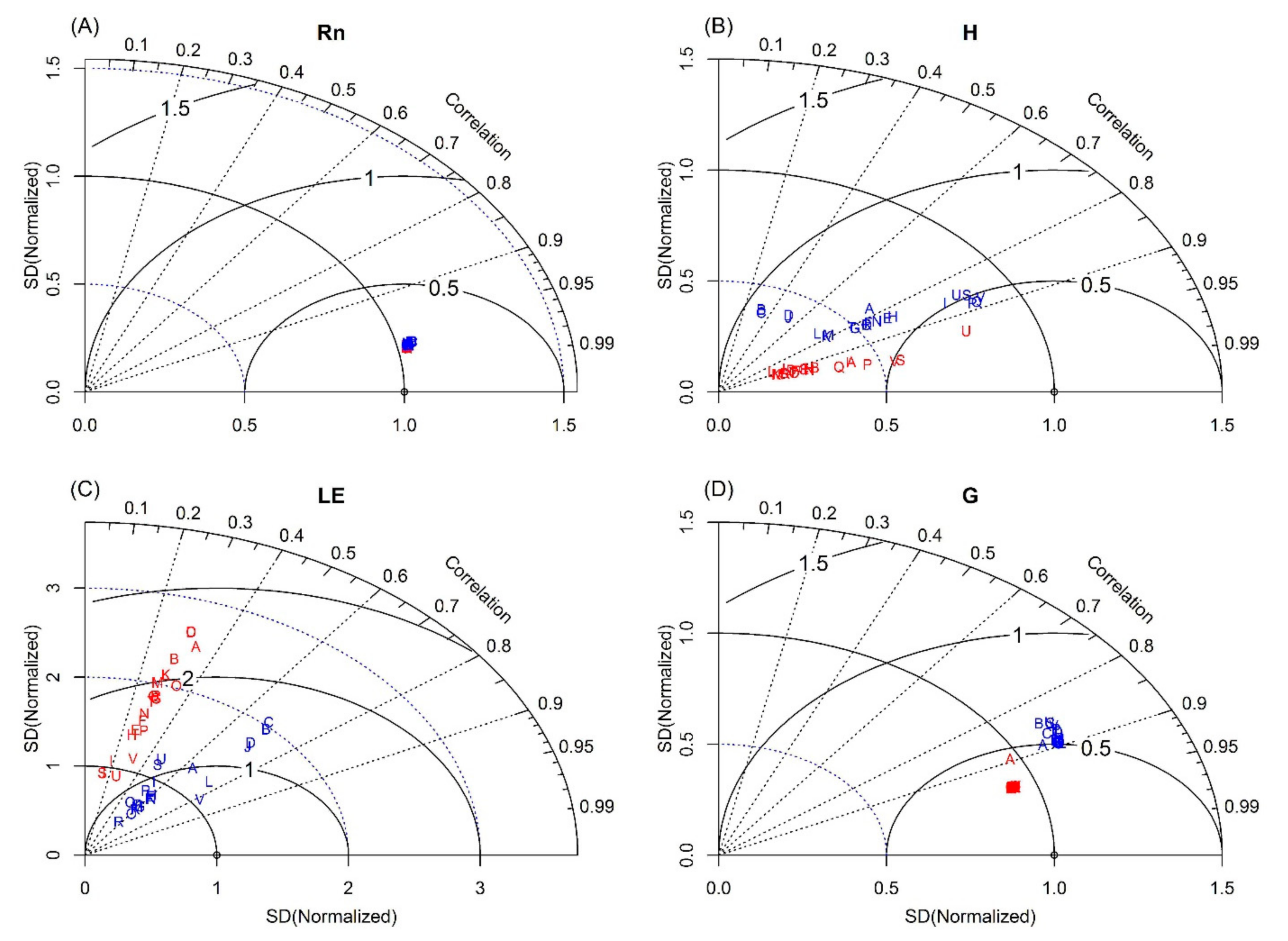
3.1. Calibration Test

For a more comprehensive verification of the simulations we elaborated Taylor diagrams, which can display the correlation, standard deviations and root mean square error between observations and multiple simulations in a single diagram. Figure 1 and Figure 2 shows the results of 44 simulations of site-scale energy balance components, as well as CO2 fluxes for the wet season (blue letters) and dry season (red letters) of 2014, compared to observations (open circles).
Initial calibrations of morphological and physiological parameters were crucial to obtain a more realistic representation of the energy fluxes in the Caatinga biome in both wet and dry seasons. Main calibrated parameters were: specific leaf area (sla), typical dimension of leaves (du), leaf width (w), coefficient of stomatal conductance (m), maximum capacity of the Rubisco enzyme (Vmax), and the initial fraction of soil moisture (θg/θd) (Table 2).
In the Taylor diagram we can observe that simulated LE and H are most sensitive to soil moisture fraction and the coefficient of stomatal conductance, mainly during the dry season (Figure 1, Table 2). For θg/θd = 0.165, the model provides a better fit between simulated LE and H and observed values in the wet season, while setting θg/θd = 0.075 results in a better fit during the dry season (Table 2). On the other hand, the NEE simulated by the model is most sensitive to the Vmax parameter (Figure 2; Table 2). When using the lowest Vmax value (40 μmol CO2 m2 s1) the SITE model underestimated NEE, while when using the highest Vmax value (120 μmol CO2 m2 s1) it overestimated NEE. The most appropriated value for Vmax was 90 μmol CO2 m2 s1 in the wet season and 60 μmol CO2 m2 s1 in the dry season (Table 2).
After analyzing the calibrated simulations through the Taylor’s diagram, we compared the ones with the higher correlation coefficient, lower RMSE and standard deviation for each season (Table 2) with non-calibrated simulations and EC observations. Table 2 shows the calibrated parameters and the best calibrated simulations in the wet season and dry season (represented by uppercase letters V, U, M and G), as analyzed by means of Taylor diagrams. For the analyses of validation, the Pearson correlation coefficient (r), median absolute error (MAE), root mean square error (RMSE) and Willmott’s index of agreement (d) was included between the modeled data with calibration by SITE model and the observation data for the years 2014 and 2015 (Table 3).

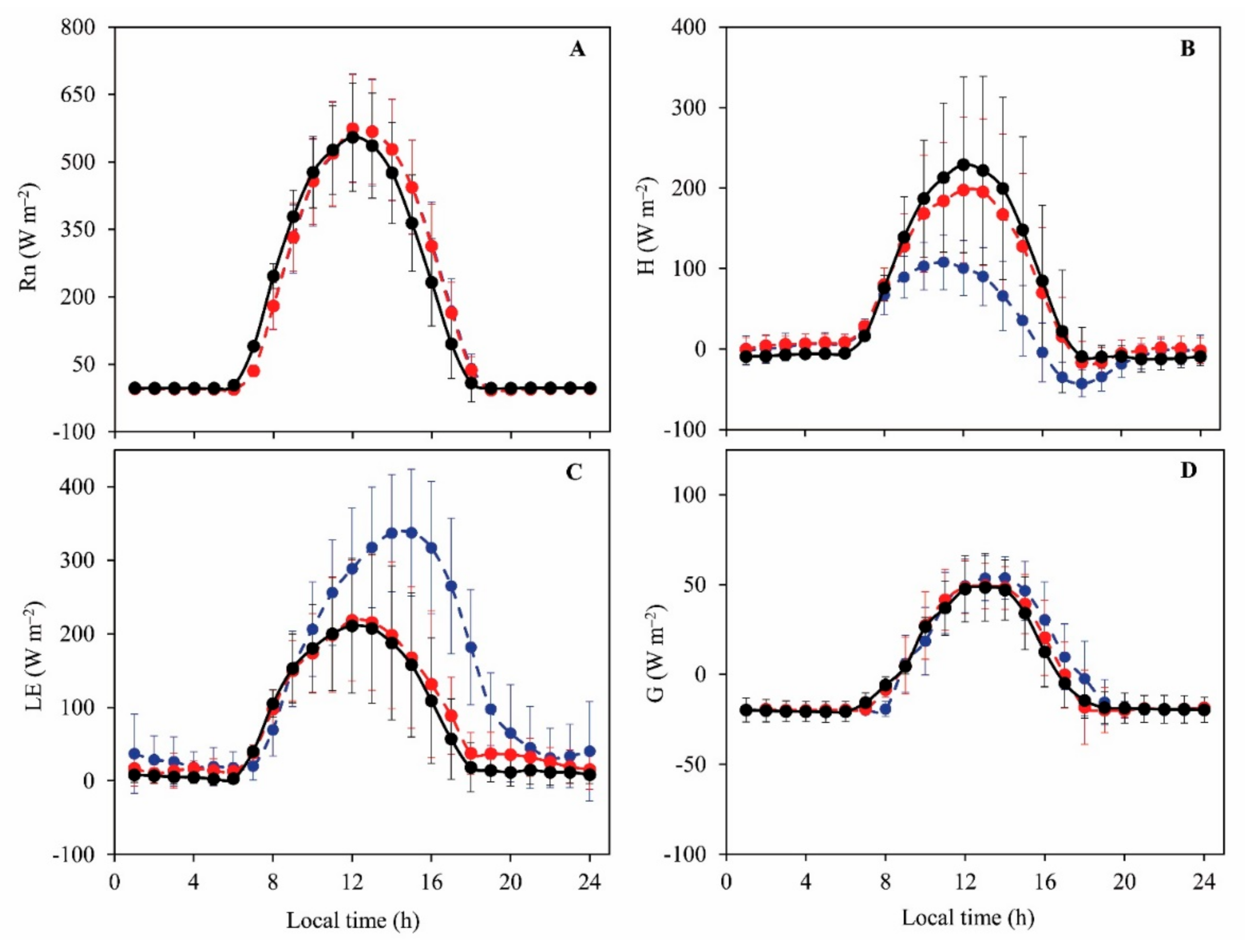
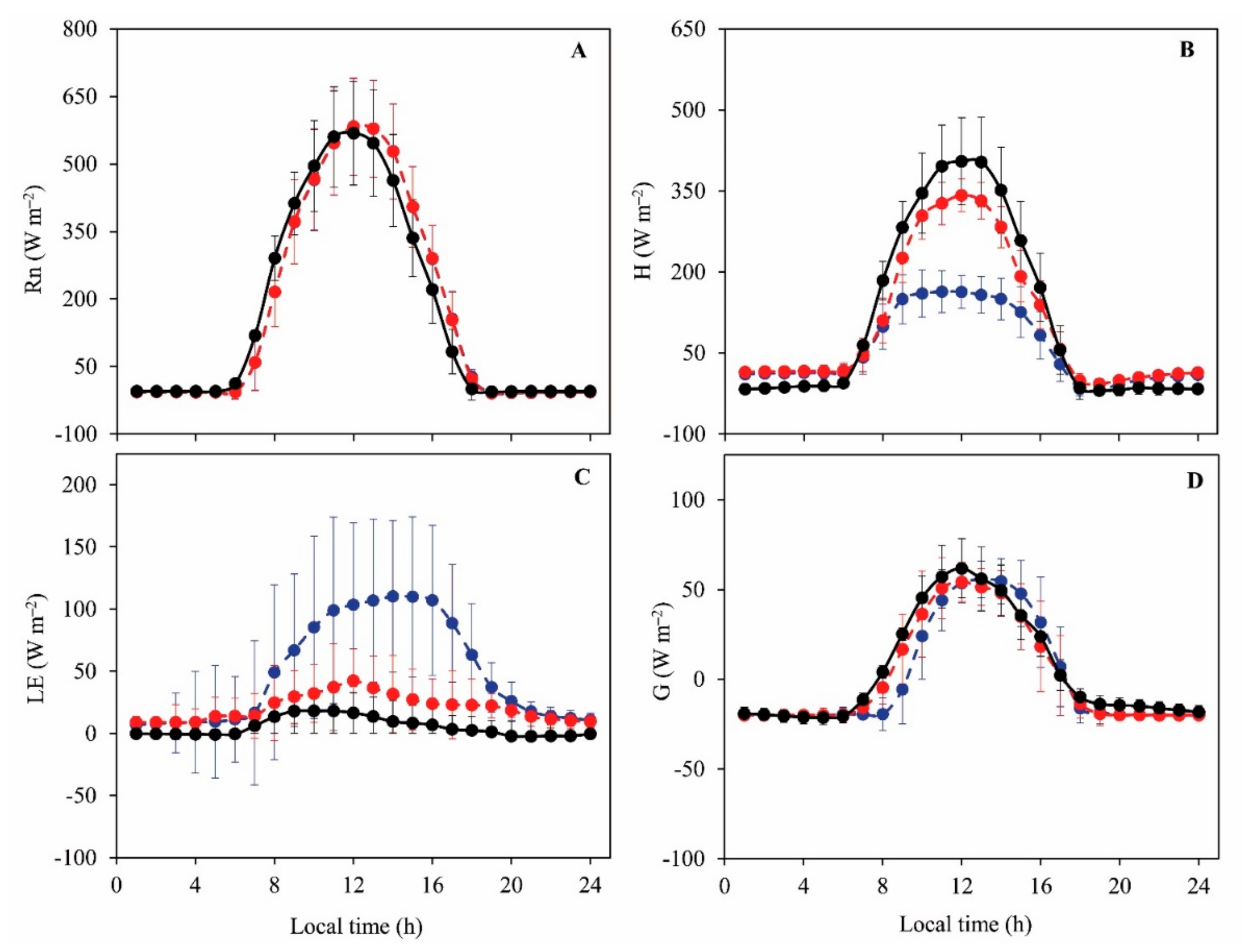
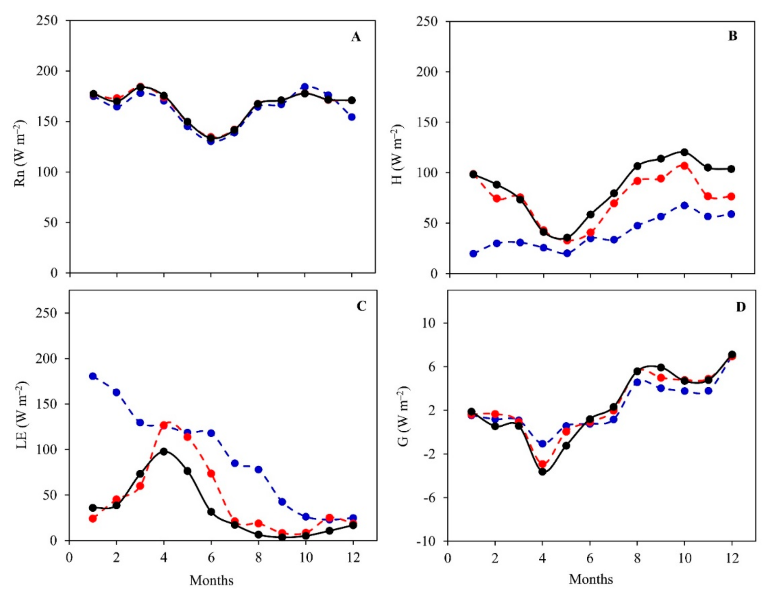
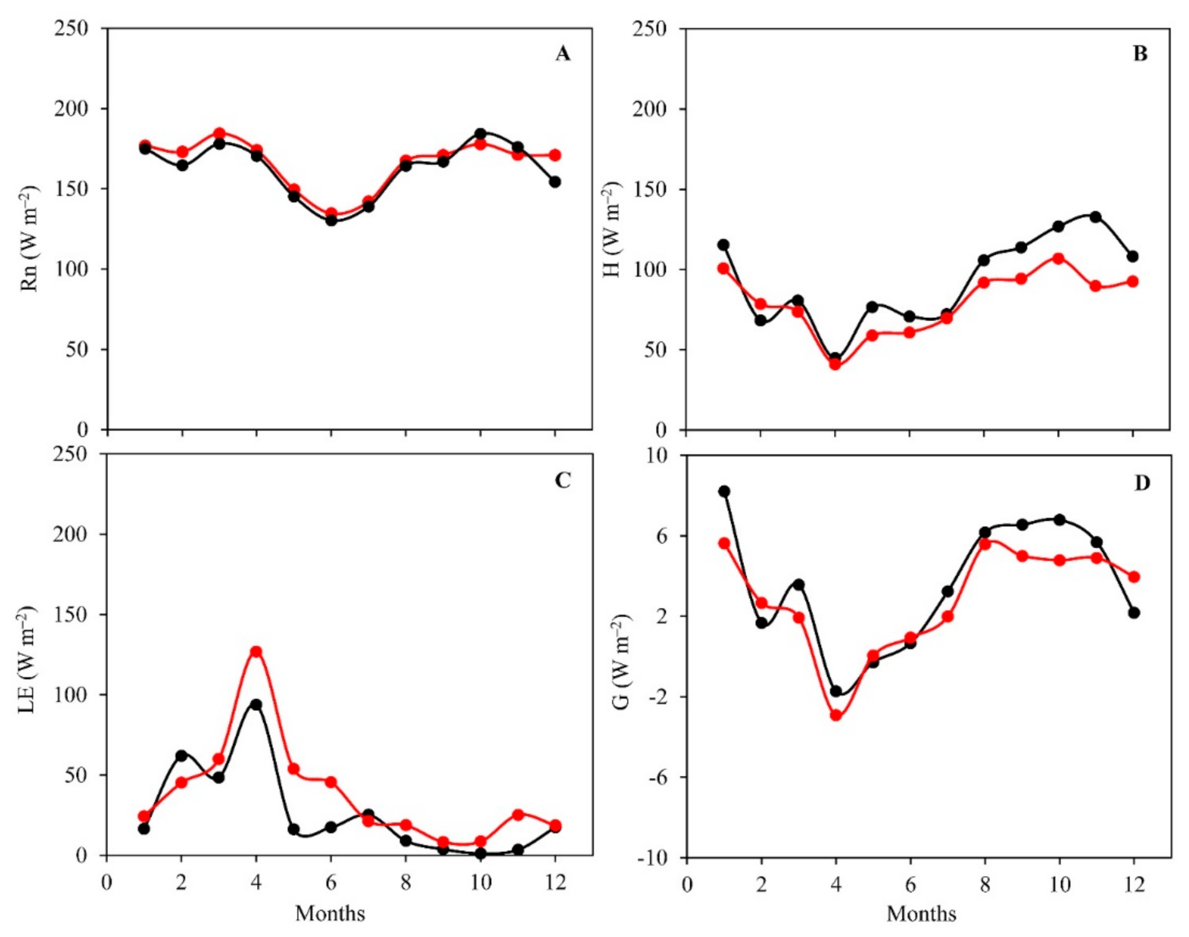
3.2. Daily Variations and Seasonal Dynamics of Simulated Energy Fluxes

Figure 3 shows the daily cycle of observed energy fluxes (solid black line), non-calibrated simulated data (dashed blue line) and calibrated simulated data (dashed red line) for Rn, H, LE and G during the wet season (February to May 2014) and Figure 4 shows the daily cycle of energy fluxes during the dry season (August to October 2014). Regarding observed values one can note that the components behave according to the daytime behavior of solar radiation, with maximum values occurring between 11h and 12h (local time). During the wet season, peak H and LE values were of 230 W m−2 and 218 W m−2, which corresponded to approximately 40% of Rn (564 W m−2), respectively (Figure 3). During the dry season, however, most of Rn (peak value of 582 W m−2) is clearly converted to H (peak value of 404 W m−2). The peak LE values are very small (20 W m−2) and the values of G and LE are approximately equivalent (Figure 4).
The non-calibrated simulation severely underestimated daily H, as much as 40% in the wet season and 66% in the dry season (Figure 3B and Figure 4B; respectively). Additionally, daily LE were overestimated by approximately 45% during the wet season and by up to 8.5 times in the dry season (Figure 3C and Figure 4C; respectively). After the calibration of the biophysical parameters (Table 2), the model satisfactorily described the daily variations of Rn, H, LE and G (r > 0.8, d > 0.7; Table 3). In general, the adjusted Rn and G were satisfactory, with r > 0.9 and d > 0.9 (Table 3). However, LE was not satisfactorily simulated (r< 0.7) in the dry season (Figure 1 and Figure 4). The main weakness of the model was in relation to the simulation of peak hours (approximately 12:00 local time), where H was underestimated in the wet season (15%) and the dry season (16%) (Figure 3 and Figure 4). On the other hand, simulated LE presented a good adjustment (r > 0.8) with observed data in the wet season, but overestimated it by approximately 35% in the dry season (Figure 4). These results indicate a certain difficulty by the model to represent variations of energy fluxes at peak times, even after exhaustive calibration tests.
The differences found between observed and simulated LE and H values during the day may be due to the fact that the model does not consider the daily variations of some parameters inherent to the ecosystem, such as the fraction of soil moisture. In the Caatinga biome, soil moisture decreases during the day, as reported by others [39,65,66]. This may explain the slight overestimation of LE after 12h00 in the wet season (Figure 3C). Similar difficulties when adjusting the hourly data variability was reported in flux simulations using the SITE model in a tropical semi-deciduous forest in the southern Amazon Basin [53] and also using other models, such as the Noah-MP, over a forest site in the Amazon [67] and integrated biosphere simulator (IBIS) for a Brazilian semiarid region [68].
The mean monthly values of the energy fluxes are presented in Figure 5and Figure 6. Table 4 shows the mean seasonal values of observed (and simulated) for the years 2014 and 2015 of the components of the energy balance. Mean seasonal Rn values ranged from 164.6 W m−2 (172.5 W m−2) and 162.6 W m−2 (173.5 W m−2) in the wet season of 2014 and 2015 to 168.7 W m−2 (167.4 W m−2) and 174.6 W m−2 (170.9 W m−2) in the dry season of 2014 and 2015, in accordance with the annual variation of solar radiation.
The mean simulated H fluxes in the wet season (58.8 W m−2 in 2014 and 67.8 W m−2 in 2015) were similar to observed values (59.7 W m−2 in 2014 and 64.6 W m−2 in 2015) (Table 4). There was a statistically significant difference between the means of H fluxes during the dry period, in which the simulated mean value was 91.9 W m−2 in 2014 and 94.4 W m−2 in 2015 while the observed value was 113.7 W m−2 and 120.0 W m−2, respectively for 2014 and 2015 (Table 4). Minimum (maximum) H (LE) values occurred during the wet season, while maximum (minimum) values occurred in the dry season. This reduction in LE and increased in H during the dry period is attributed to lower water availability in the soil due to the absence of rainfall over the Caatinga biome. In addition, we verified a statistically significant difference between simulated and observed LE mean values in the dry period (Table 4). Table 3 shows that the error statistics of H and LE between eddy covariance observations and simulations with the parameters set after calibration for the years 2014 and 2015 (values in parenthesis) presented a MAE value of 50.52(46.94), RMSE 68.83(71.97), r 0.85(0.91) and d 0.89(0.89) for H, and MAE value of 29.97(24.25), RMSE 65.99(53.48), r 0.69(0.74) and d 0.72(0.74) for LE. In general, mean seasonal G values were low, less than 10.0 W m−2 and with a monthly variability similar to that featured by H. The highest G values occurred during the dry season, period in which leaf senescence occurs in the Caatinga and the soil is more exposed to radiation. The analysis of G fluxes simulated by the model showed no statistically significant difference between simulated and observed values (Table 4).
Both the underestimation and overestimation of H and LE retrieved using the non-calibrated model (dashed blue lines, Figure 5) were greatly reduced with the adjustment of the SITE model according to specific wet season and dry season parameters (Figure 5 and Figure 6). The model was run twice, and the specific forecasts of each season were merged. These discrepancies in the non-calibrated model happened mainly because under conditions of low water availability a higher portion of the net solar radiation is converted to H. Our results were consistent with observational analysis in a tropical semi-deciduous forest in the southern Amazon Basin performed according to the literature [53]. These authors reported that LE was overestimated by 40% and H was underestimated by 66%. The discrepancy between observed and simulated H and LE values was observed in other studies using the SITE model in the Amazon rainforest [35] and also using other models in other ecosystems, such as temperate grasslands [69].
As discussed in the literature [70], throughout the annual cycle, LE behaves as a function of annual mean rainfall due to water limitations observed in tropical savanna ecosystems during the dry season. In addition, the energy flux partition is directly associated to vegetation characteristics and land use changes [16,33]. The occurrence of higher H values in arid and semiarid regions is a consequence of the reduction in water availability caused by low rainfall in these regions. Some studies show that in the Caatinga most of the available energy is converted into sensible heat flux in the dry season [33,34]. A similar trend of decreasing LE during the dry season was reported in the literature [34], which studied energy balance components in a preserved Caatinga region. These mechanisms of LE variability were satisfactorily simulated in the present study.
During the months with low water availability, the non-calibrated model greatly underestimates H. The default input parameters probably lead to the simulation of an ecosystem facing a higher water stress in relation to the Caatinga observational data. Thus, the use of specific parameters (e.g., reduced initial fraction of soil moisture—θg/θd) during the calibration of the model was necessary to improve its performance in simulating LE. The same issue when adjusting variations in H and LE values during the dry season was reported for simulations of energy fluxes using the SITE model in a semi-deciduous tropical forest in the Amazon [53].
The seasonality of rainfall and light greatly affect leaf morphology and physiology in the Caatinga species. During the dry season, the Caatinga vegetation, which consists primarily of deciduous and semi-deciduous species, reaches its minimum level of physiological activity, which in turn is barely sufficient for the maintenance of leaves. Indeed, leaves become shorter, narrower and smaller, leading to a significant decrease in the specific leaf area [61,63]. Under these conditions, transpiration rates in the Caatinga are very close zero [62,71]. The direct effect of these characteristics is the reduction of LE, with Rn being mostly converted into H.

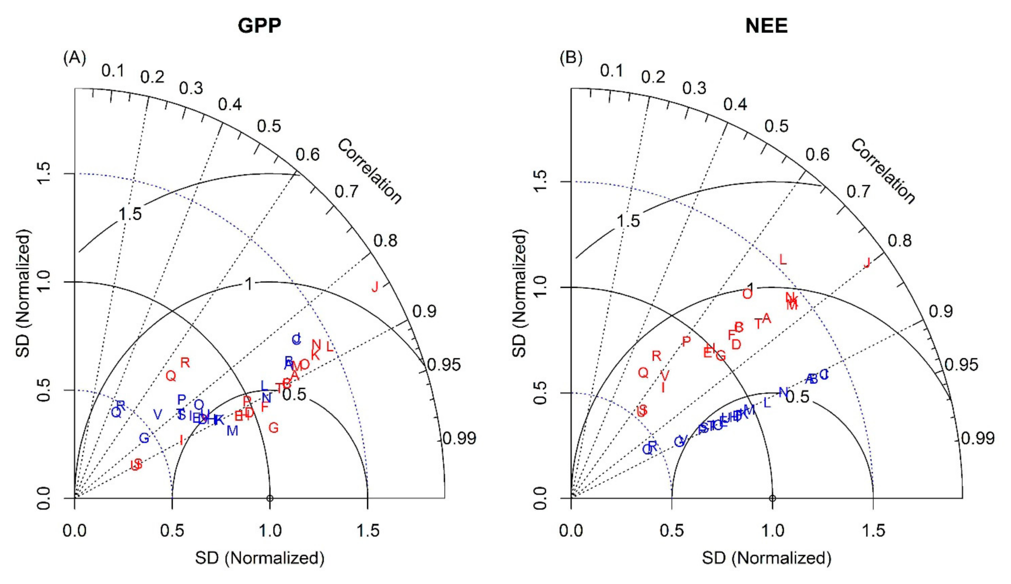
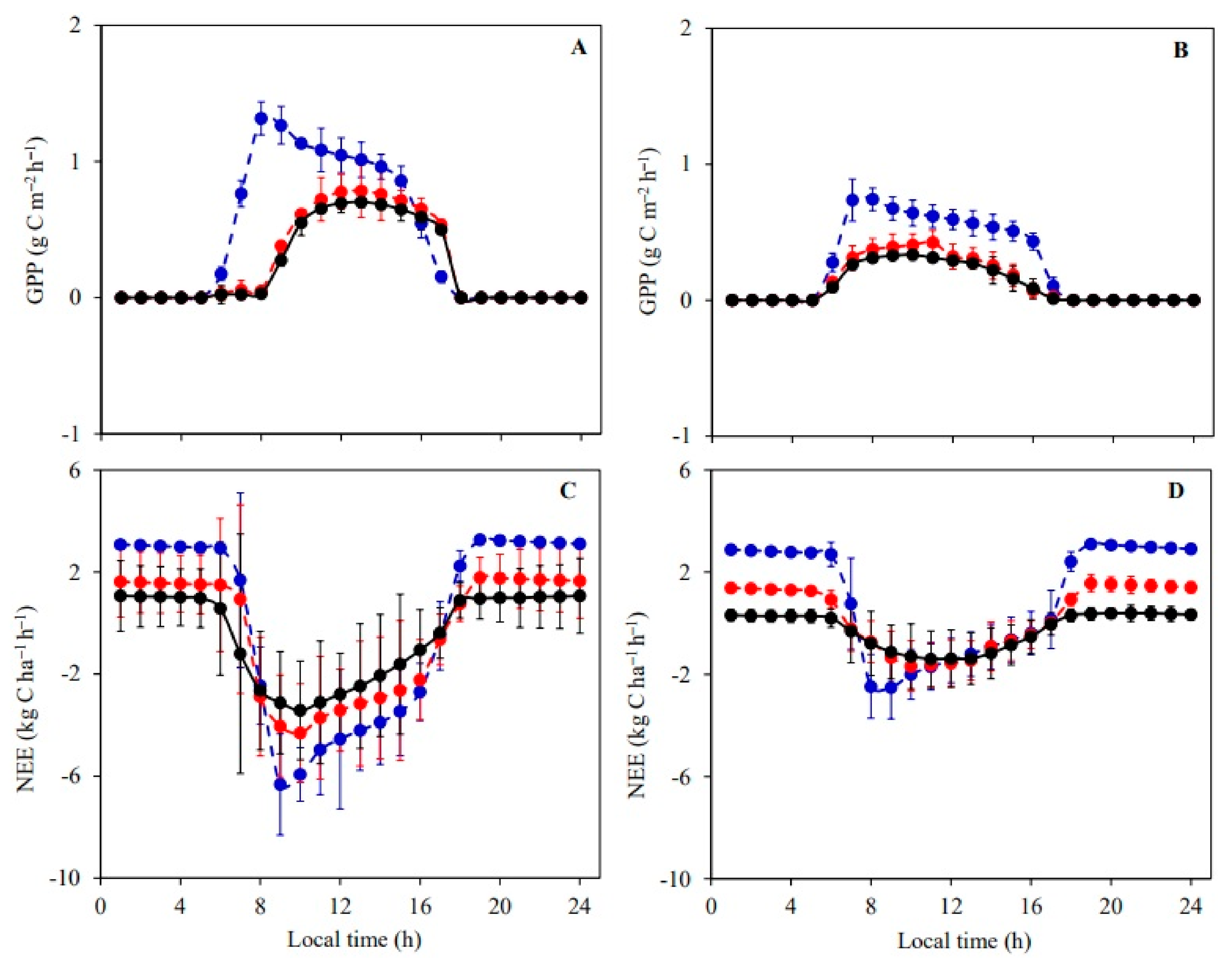
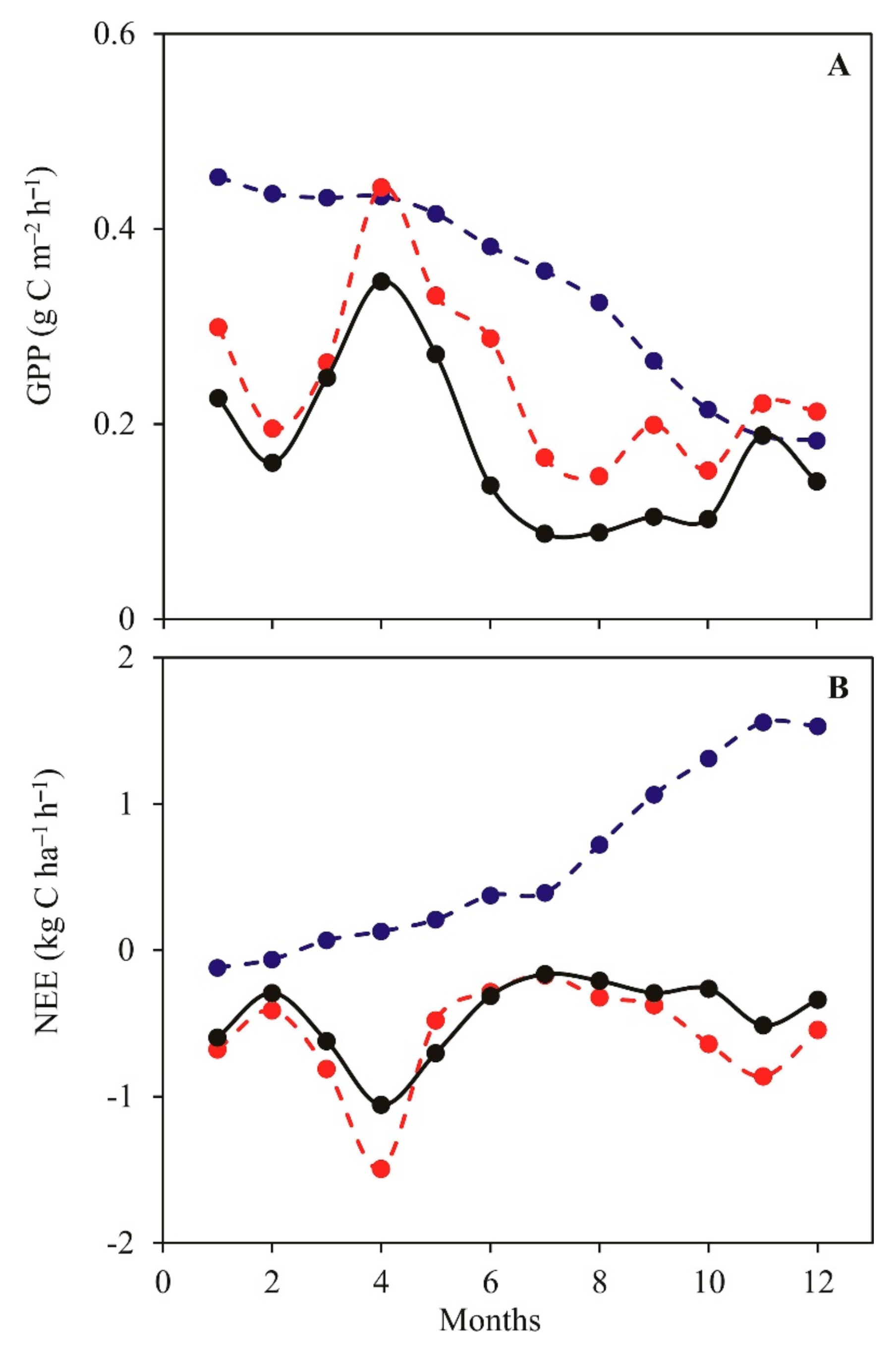
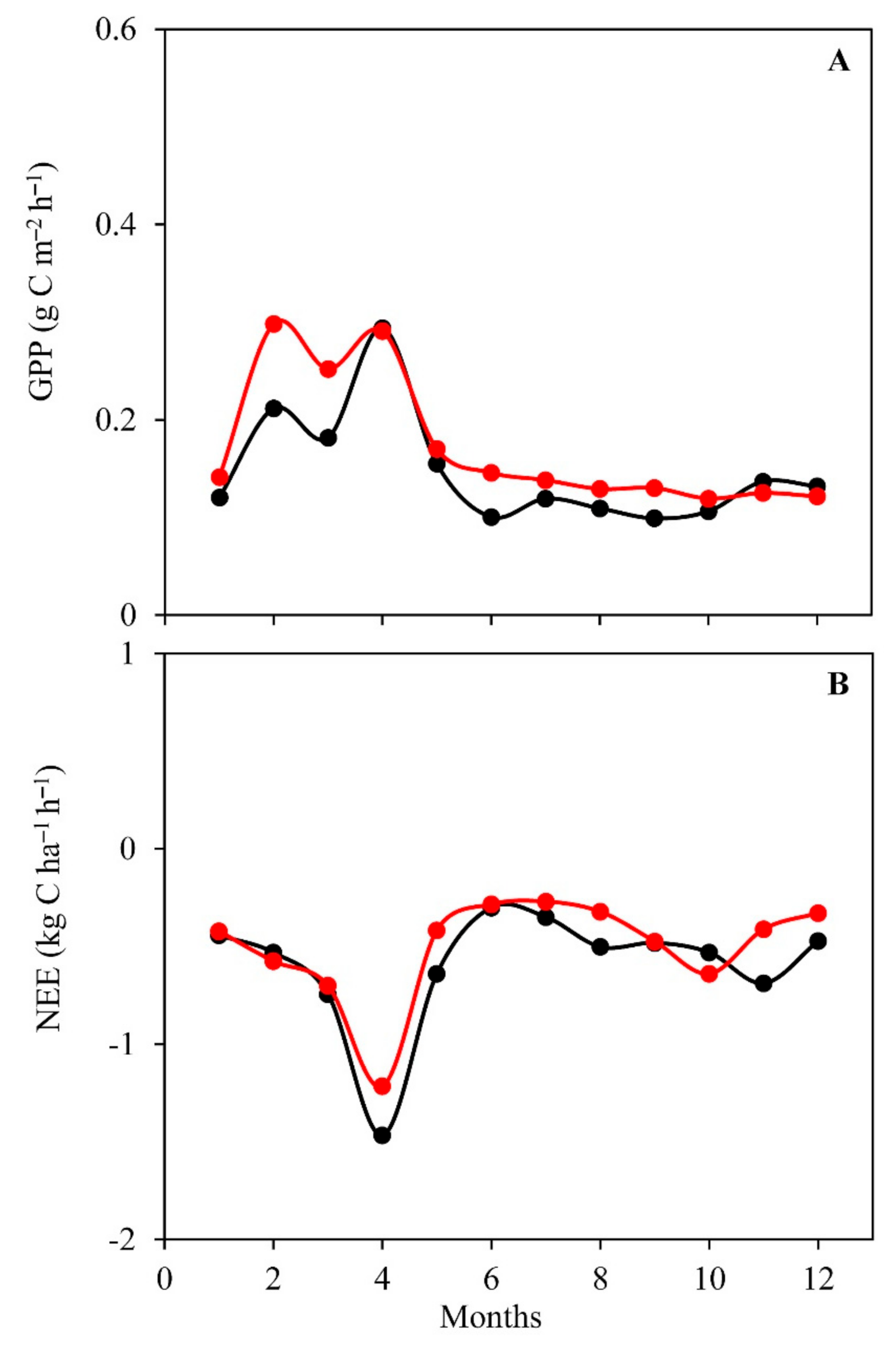
3.3. Daily Variations and Seasonal Dynamics of Simulated CO2 Fluxes

Figure 7 shows the daily variations in observed and simulated GPP and NEE, considering both non-calibrated simulations and the simulations with the best calibration for the wet and dry seasons. The observed GPP and NEE values presented a pronounced daily cycle, with larger amplitude during the wet season and smaller amplitude during the dry season (Figure 7), indicating that carbon uptake was more intense in the wet season due to the higher water availability. The observed GPP and NEE values sharply increased after sunrise, reaching maximum values between 09h and 11h and declining after noon, reaching its lowest values (near zero) at the end of the afternoon.
The non-calibrated simulations greatly overestimated the mean daily cycle values during both seasons (Figure 7). This illustrates the effect of neglecting the contribution of the physiological and morphological parameters of plants in this environment when predicting CO2 fluxes. The main parameter influencing NEE and GPP was Vmax. Using a value of 90 μmol CO2 m2 s1 for the wet season and 60 μmol CO2 m2 s1 for the dry season resulted in a fair agreement with observed values and a reasonable consistence with values obtained in previous ecophysiological studies involving species of the Caatinga [4,62,64].
In comparison with data from others research, we can observe that most of the modeling studies neglect the phenological variation of the ecosystems, usually considering a single value for Vmax. For example, the values used in the Biosphere Energy Transfer and Hydrology model—BETHY [72] and in the global-scale mechanistic model HYBRID [73], 65 and 51 μmol CO2 m2 s1, respectively, are similar to the dry season Vmax used in the present study. In contrast, the values of Vmax defined for the joint UK land environment simulator model—JULES [74,75] and community land model—CLM [76] are lower (48 and 31 μmol CO2 m2 s1, respectively) if compared to Vmax values used in other models. As reported in the literature [64] after calibrating Vmax (approximately 90 μmol CO2 m2 s1) values for the Caatinga in dynamic global vegetation models (DGVM), simulation results reached 72% of total observed GPP.
Simulations of GPP and NEE were also sensitive to changes in the coefficient of stomatal conductance, specific leaf area, typical dimension of leaves and leaf width (Table 2). The study [77] used a dimensional model for forest canopy radiation absorption, photosynthesis, and transpiration (MAESTRA) to estimate GPP in the Amazon Forest, showing that modeled GPP was sensitive to changes in total canopy leaf area and Vmax, and that soil moisture, in addition to vapor pressure, controlled canopy CO2 fluxes during drought periods.
The simulation also accurately retrieved the time at which the daily NEE peak occurs, between 09 h and 11 h. As presented in the previous study [35] using the SITE model, obtained a correlation coefficient of 0.88 between simulated and observed hourly CO2 fluxes in a primary tropical evergreen forest, while in the literature [78] using two versions of the SSiB model in Amazon region, obtained correlation coefficients of 0.73 and 0.79 between observed and simulated hourly CO2 fluxes.
The NEE is the difference between soil heterotrophic respiration and net primary production, thus negative NEE values indicate assimilation of carbon by the ecosystem. Furthermore, net primary production is GPP (gross photosynthesis) minus autotrophic respiration. NEE is highly dependent on stomatal opening, since stomatal conductance is commonly the main determining factor in CO2 fixation [79,80]. In addition, biochemical models of photosynthesis (PN) show that PN represents the minimum value of two limiting factors: maximum carboxylation rates of Rubisco (Vmax) and electron transport rate (Jmax) [81]. Thus, the decline in GPP and NEE after 11h can be explained by the influence of environmental factors on the stomatal opening and biochemical parameters of photosynthesis such as kinetics of the Rubisco enzyme [4,80].
One noteworthy exception in the accuracy of the model refers to the nighttime period (Figure 7C,D). Values of CO2 fluxes during nighttime were overestimated by 48% (wet season) and 56% (dry season), leading to higher RMSE (2.25) and MAE (1.99) of NEE relatively to GPP, which presented RMSE of 1.53 and MAE was 1.24 (Table 3). Have been previously reported [9] that the sensitivity of soil-surface CO2 fluxes to volumetric water content above 10 cm is probably closely related to a high percentage of root and microbial biomasses in the 0–10 cm profile of tallgrass prairie. Therefore, the overestimation of simulated night CO2 fluxes can be explained by the combination of root metabolism, root exudation, and, consequently, microbial activity in the rhizosphere.
Figure 8 and Figure 9 shows of monthly mean values of CO2 fluxes in 2014 and 2015, respectively, evidencing the existence of a clear seasonal variability. Table 4 shows means seasonal values of observed (and simulated) for the years 2014 and 2015 of GPP and NEE. The GPP and NEE increased at the onset of the wet season and reaching peak values in April 2014 and 2015, which GPP declined until reaching values lower than 0.2 g C m−2 h−1 in the dry season. Mean seasonal GPP in 2014 varied from 0.11 g C m−2 h−1 (0.17 g C m−2 h−1) (dry season) to 0.26 g C m−2 h−1 (0.29 g C m−2 h−1) in the wet season (Table 4). In 2015, GPP values presented a similar trend, ranging from 0.10 g C m−2 h−1 (0.12 g C m−2 h−1) (dry season) to 0.20 g C m−2 h−1 (0.25 g C m−2 h−1) in the wet season (Table 4). The simulation was able to capture the GPP and NEE seasonal variability. This result may indicate an efficiency of the SITE model in representing of gross primary production (GPP) and net ecosystem CO2 exchange (NEE) dynamics in the Caatinga environment.
In the wet season, climate, canopy, and soil water conditions were optimal for the Caatinga vegetation. Thus, the GPP and NEE peaked and surface energy exchange was driven mainly by LE, while H was low. Photosynthetic activity decreased at the onset of the dry season because the soil was dry, leaf senescence occurred and H dominated surface energy exchange. In other words, water stress modulates the variations in canopy CO2 fluxes throughout the seasons. The increase in rainfall rates in the wet season favors CO2 uptake resulting in increased GPP and NEE in the Caatinga. In contrast, a reduction in soil moisture content induces stomatal closure and might affect some photosynthetic traits such as the Rubisco kinetics—Vmax [82].
Furthermore, the effects of drought in the GPP and NEE could not be captured by the SITE model unless the calibration for the dry season was carried out. These results demonstrate that net CO2 fluxes are very sensitive to the physiological processes that control surface energy exchange. Moreover, differences between seasonal observational and modeled carbon pools highlight the importance of phenology as an essential tool for understanding productivity in Caatinga. Others researches also report the importance of phenology in the dynamic of global vegetation models [83,84].

4. Conclusions

This study evaluated the performance of the SITE model when incorporated with parameters and input data consistent with in situ observations from the Caatinga biome, which is a seasonally dry tropical forest in the Brazilian semiarid region. In general, the SITE model exhibited reasonable applicability to simulate variations in CO2 and energy fluxes. We believe that the SITE model could be used to simulate a satisfactory vegetation response if we take into consideration the remarkable phenological seasonality of the Caatinga. The LE flux was the output variable with the most unsatisfactory adjustment, overestimating observed values in the dry season. Furthermore, our ecophysiological approach offers the possibility to explore morphoanatomical and physiological mechanisms determinants of GPP and NEE in the Caatinga biome. Evaluating and improving the representation of the vegetation structure, dynamics, energy and carbon cycle of the Caatinga in vegetation models will help further develop our understanding on the impacts of land-use changes on regional and global carbon cycle.

Author Contributions

Conceptualization, K.R.M., B.G.B. and C.M.S.e.S.; methodology, K.R.M., B.G.B., C.M.S.e.S., S.C., R.R.F., T.M.R., T.V.M., J.S.d.R., M.M.d.L.V., A.C.N.S., A.M.S.M., D.T.C.d.S. and D.F.d.S.; validation, K.R.M., B.G.B. and C.M.S.e.S.; formal analysis, P.R.M., C.P.O., W.A.G., G.B.C., M.F.P., R.A.M., A.C.D.A. and R.S.C.M.; investigation, K.R.M., B.G.B. and C.M.S.e.S.; writing—original draft preparation, K.R.M.; writing—review and editing, K.R.M., B.G.B., C.M.S.eS, P.R.M., G.B.C., R.A.M., C.P.O. and W.A.G. All authors have read and agreed to the published version of the manuscript.

Funding

This research was funded by National Council for Scientific and Technological Development (CNPq), Process nº 303802/2017-0 and National Observatory of Water and Carbon Dynamics in the Caatinga Biome (INCT -MCTI/CNPq/CAPES/FAPs 16/2014, grant: 465764/2014-2 and MCTI/CNPq Nº 28/2018, grant 420854/2018-5).

Institutional Review Board Statement

Not applicable.

Informed Consent Statement

Not applicable.

Data Availability Statement

The data presented in this study are available on request from the corresponding author. The data are not publicly available due to privacy.

Acknowledgments

The authors are thankful to the Brazilian National Institute of Semi-Arid (INSA) for funding the project which originated the EC data used in this study. We are also thankful to ICMBio (Chico Mendes Institute for Biodiversity Conservation) for providing access to the experimental site and to ESEC-Seridó (Ecological Station of Seridó) for supporting experimental activities. The authors are also thankful to the Coordination for the Improvement of Higher Education Personnel (CAPES) for the postdoctoral funding granted to the first author. This work was partially supported by the high-performance computing facilities of NPAD/UFRN. Finally, we are thankful to the National Council for Scientific and Technological Development (CNPq) for the research productivity grant of the last author (Process nº 303802/2017-0) and the financial support in the NOWCDCB project: National Observatory of Water and Carbon Dynamics in the Caatinga Biome (INCT -MCTI/CNPq/CAPES/FAPs 16/2014, grant: 465764/2014-2 and MCTI/CNPq Nº 28/2018, grant 420854/2018-5).

Conflicts of Interest

The authors declare no conflict of interest.

References

  1. Glotfelty, T.; Zhang, Y. Impact of future climate policy scenarios on air quality and aerosol–cloud interactions using an advanced version of CESM/CAM5: Part II. Future trend analysis and impacts of projected anthropogenic emissions. Atmos. Environ. 2017, 152, 531–552. [Google Scholar] [CrossRef] [Green Version]
  2. Parmesan, C.; Burrows, M.T.; Duarte, C.M.; Poloczanska, E.S.; Richardson, A.J.; Schoeman, D.S.; Singer, M.C. Beyond climate change attribution in conservation and ecological research. Ecol. Lett. 2013, 16, 58–71. [Google Scholar] [CrossRef] [PubMed]
  3. Sá, J.C.D.M.; Lal, R.; Cerri, C.C.; Lorenz, K.; Hungria, M.; Carvalho, P.C.D.F. Low-carbon agriculture in South America to mitigate global climate change and advance food security. Environ. Int. 2017, 98, 102–112. [Google Scholar] [CrossRef] [PubMed] [Green Version]
  4. Dombroski, J.L.D.; Praxedes, S.C.; Freitas, R.M.O.; Pontes, F.M. Water relations of Caatinga trees in the dry season. S. Afr. J. Bot. 2011, 77, 430–434. [Google Scholar] [CrossRef] [Green Version]
  5. Santos, M.G.; Oliveira, M.T.; Figueiredo, K.V.; Falcão, H.M.; Arruda, E.C.P.; De Almeidacortez, J.S.; Sampaio, E.V.S.B.; Ometto, J.P.H.B.; Menezes, R.S.C.; Oliveira, A.F.M.; et al. Caatinga, the Brazilian dry tropical forest: Can it tolerate climate changes? Theor. Exp. Plant Physiol. 2014, 26, 83–99. [Google Scholar] [CrossRef]
  6. Koch, R.; Almeida–Cortez, J.S.; Kleinschmit, B. Revealing areas of high nature conservation importance in a seasonally dry tropical forest in Brazil: Combination of modelled plant diversity hot spots and threat patterns. J. Nat. Conserv. 2017, 35, 24–39. [Google Scholar] [CrossRef]
  7. Foley, J.A.; Prentice, I.C.; Ramankutty, N.; Levis, S.; Pollard, D.; Sitch, S.; Haxeltine, A. An integrated biosphere model of land surface processes, terrestrial carbon balance, and vegetation dynamics. Glob. Biogeochem. Cycles 1996, 10, 603–628. [Google Scholar] [CrossRef]
  8. Luyssaert, S.; Inglima, I.; Jung, M.; Richardson, A.D.; Reichstein, M.; Papale, D.; Piao, S.L.; Schulze, E.; Wingate, L.; Matteucci, G.; et al. CO2 balance of boreal, temperate, and tropical forests derived from a global database. Glob. Chang. Biol. 2007, 13, 2509–2537. [Google Scholar] [CrossRef] [Green Version]
  9. Bremer, D.J.; Ham, J.M. Measurement and modeling of soil CO2 flux in a temperate grassland under mowed and burned regimes. Ecol. Appl. 2002, 12, 1318–1328. [Google Scholar]
  10. Hao, Y.; Wang, Y.; Huang, X.; Cui, X.; Zhou, X.; Wang, S.; Niu, H.; Jiang, G. Seasonal and interannual variation in water vapor and energy exchange over a typical steppe in Inner Mongolia, China. Agric. For. Meteorol. 2007, 146, 57–69. [Google Scholar] [CrossRef]
  11. Musavi, T.; Migliavacca, M.; Reichstein, M.; Kattge, J.; Wirth, C.; Black, T.A.; Janssens, I.; Knohl, A.; Loustau, D.; Roupsard, O.; et al. Stand age and species richness dampen interannual variation of ecosystem-level photosynthetic capacity. Nat. Ecol. Evol. 2017, 1, 0048. [Google Scholar] [CrossRef] [PubMed] [Green Version]
  12. Post, W.M.; Kwon, K.C. Soil carbon sequestration and land–use change: Processes and potential. Glob. Chang. Biol. 2000, 6, 317–327. [Google Scholar] [CrossRef] [Green Version]
  13. Biudes, M.S.; Vourlitis, G.L.; Machado, N.G.; de Arruda, P.H.Z.; Neves, G.A.R.; de Almeida Lobo, F.; Neale, C.M.U.; de Souza Nogueira, J. Patterns of energy balance exchange for tropical ecosystems across a climate gradient in Mato Grosso, Brazil. Agric. For. Meterol. 2015, 202, 112–124. [Google Scholar] [CrossRef]
  14. Cabral, O.M.R.; Rocha, H.R.; Gash, J.H.; Freitas, H.C.; Ligo, M.A.V. Water and energy fluxes from woodland savanna (cerrado) in southeast Brazil. J. Hydrol. Reg. Stud. 2015, 4, 22–40. [Google Scholar] [CrossRef] [Green Version]
  15. Campos, S.; Mendes, K.R.; Da Silva, L.L.; Mutti, P.R.; Medeiros, S.S.; Amorim, L.B.; Dos Santos, C.A.; Perez-Marin, A.M.; Ramos, T.M.; Marques, T.V.; et al. Closure and partitioning of the energy balance in a preserved area of a Brazilian seasonally dry tropical forest. Agric. For. Meteorol. 2019, 271, 398–412. [Google Scholar] [CrossRef]
  16. Silva, P.F.; de Sousa Lima, J.R.; Antonino, A.C.D.; Souza, R.; de Souza, E.S.; Silva, J.R.I.; Alves, E.M. Seasonal patterns of carbon dioxide, water and energy fluxes over the Caatinga and grassland in the semi-arid region of Brazil. J. Arid. Environ. 2017, 147, 71–82. [Google Scholar] [CrossRef]
  17. Meir, P.; Metcalfe, D.B.; Costa, A.C.L.; Fisher, R.A. The fate of assimilated carbon during drought: Impacts on respiration in Amazon rainforests. Philos. Trans. R. Soc. B. 2008, 363, 1849–1855. [Google Scholar] [CrossRef]
  18. Sotta, E.D.; Veldkamp, E.; Schwendenmann, L.; Guimarães, B.R.; Paixão, R.K.; Ruivo, M.D.L.P.; Da Costa, A.C.L.; Meir, P. Effects of an induced drought on soil carbon dioxide (CO2) efflux and soil CO2 production in an Eastern Amazonian rainforest, Brazil. Glob. Chang. Biol. 2007, 13, 2218–2229. [Google Scholar] [CrossRef]
  19. Wu, J.; Guan, K.; Hayek, M.N.; Coupe, N.R.; Wiedemann, K.T.; Xu, X.; Wehr, R.; Christoffersen, B.O.; Miao, G.; Da Silva, R.; et al. Partitioning controls on Amazon forest photosynthesis between environmental and biotic factors at hourly to interannual timescales. Glob. Chang. Biol. 2016, 23, 1240–1257. [Google Scholar] [CrossRef]
  20. Zeri, M.; Sá, L.D.D.A.; Manzi, A.O.; Araújo, A.C.; Aguiar, R.G.; Von Randow, C.; Sampaio, G.; Cardoso, F.L.; Nobre, C.A. Variability of Carbon and Water Fluxes Following Climate Extremes over a Tropical Forest in Southwestern Amazonia. PLoS ONE 2014, 9, e88130. [Google Scholar] [CrossRef] [Green Version]
  21. Barbosa, H.A.; Kumar, T.V.L. Influence of rainfall variability on the vegetation dynamics over Northeastern Brazil. J. Arid Environ. 2016, 124, 377–387. [Google Scholar] [CrossRef]
  22. Mendes, K.R.; Campos, S.; Da Silva, L.L.; Mutti, P.R.; Ferreira, R.R.; Medeiros, S.S.; Perez-Marin, A.M.; Marques, T.V.; Ramos, T.M.; Vieira, M.M.D.L.; et al. Seasonal variation in net ecosystem CO2 exchange of a Brazilian seasonally dry tropical forest. Sci. Rep. 2020, 10, 1–16. [Google Scholar] [CrossRef] [PubMed]
  23. Cunha, A.P.M.A.; Alvalá, R.C.; Kubota, P.Y.; Vieira, R.M. Impacts of land use and land cover changes on the climate over Northeast Brazil. Atmos. Sci. Lett. 2015, 16, 219–227. [Google Scholar] [CrossRef]
  24. De Souza, D.C.; Oyama, M.D. Climatic consequences of gradual desertification in the semi–arid area of Northeast Brazil. Theor. Appl. Climatol. 2011, 103, 345–357. [Google Scholar] [CrossRef]
  25. Marengo, J.A.; Ambrizzi, T.; Da Rocha, R.P.; Alves, L.M.; Cuadra, S.V.; Valverde, M.C.; Torres, R.R.; Santos, D.C.; Ferraz, S.E.T. Future change of climate in South America in the late twenty-first century: Intercomparison of scenarios from three regional climate models. Clim. Dyn. 2010, 35, 1073–1097. [Google Scholar] [CrossRef]
  26. Marengo, J.A.; Torres, R.R.; Alves, L.M. Drought in Northeast Brazil—Past, present, and future. Theor. Appl. Climatol. 2017, 129, 1189–1200. [Google Scholar] [CrossRef]
  27. Beer, C.; Reichstein, M.; Tomelleri, E.; Ciais, P.; Jung, M.; Carvalhais, N.; Rödenbeck, C.; Arain, M.A.; Baldocchi, D.; Bonan, G.B.; et al. Terrestrial gross carbon dioxide uptake: Global distribution and covariation with climate. Science 2010, 329, 834–838. [Google Scholar] [CrossRef] [Green Version]
  28. Cleverly, J.; Eamus, D.; Van Gorsel, E.; Chen, C.; Rumman, R.; Luo, Q.; Coupe, N.R.; Li, L.; Kljun, N.; Faux, R.; et al. Productivity and evapotranspiration of two contrasting semiarid ecosystems following the 2011 global carbon land sink anomaly. Agric. For. Meteorol. 2016, 220, 151–159. [Google Scholar] [CrossRef] [Green Version]
  29. Tang, X.; Carvalhais, N.; Moura, C.; Ahrens, B.; Koirala, S.; Fan, S.; Reichstein, M. Global variability of carbon use efficiency in terrestrial ecosystems. Biogeosci. Discuss. 2019. [Google Scholar] [CrossRef] [Green Version]
  30. Jaeger, E.B.; Stöckli, R.; Seneviratne, S.I. Analysis of planetary boundary layer fluxes and land–atmosphere coupling in the regional climate model CLM. J. Geophys. Res. 2009, 114, D17106. [Google Scholar] [CrossRef] [Green Version]
  31. Von Randow, C.; Zeri, M.; Coupe, N.R.; Muza, M.N.; De Goncalves, L.G.G.; Costa, M.H.; Araújo, A.C.; Manzi, A.O.; Da Rocha, H.R.; Saleska, S.R.; et al. Inter-annual variability of carbon and water fluxes in Amazonian forest, Cerrado and pasture sites, as simulated by terrestrial biosphere models. Agric. For. Meteorol. 2013, 182-183, 145–155. [Google Scholar] [CrossRef]
  32. Pires, W.N.; Moura, M.S.B.; Souza, L.S.B.; Silva, T.G.F.; Carvalho, H.F.S. Fluxos de radiação, energia, CO2 e vapor de água em uma área de caatinga em regeneração. Agrometoeros 2017, 25, 143–151. (In Portuguese) [Google Scholar]
  33. Souza, R.; Feng, X.; Antonino, A.; Montenegro, S.; Souza, E.; Porporato, A. Vegetation response to rainfall seasonality and interannual variability in tropical dry forests. Hydrol. Process. 2016, 30, 3583–3595. [Google Scholar] [CrossRef]
  34. Teixeira, A.H.C.; Bastiaanssen, W.G.M.; Ahmad, M.D.; Moura, M.S.B.; Bos, M.G. Analysis of energy fluxes and vegetation–atmosphere parameters in irrigated and natural ecosystems of semi–arid Brazil. J. Hydrol. 2008, 362, 110–127. [Google Scholar] [CrossRef] [Green Version]
  35. Santos, S.N.M.; Costa, M.H. A simple tropical ecosystem model of carbon, water and energy fluxes. Ecol. Model. 2004, 176, 291–312. [Google Scholar] [CrossRef]
  36. Tavares-Dasmasceno, J.P.; de Souza Silveira, J.L.G.; Câmara, T.; de Castro Stedile, P.; Macario, P.; Toledo-Lima, G.S.; Pichorim, M. Effect of drought on demography of Pileated Finch (Coryphospingus pileatus: Thraupidae) in northeastern Brazil. J. Arid Environ 2017, 147, 63–79. [Google Scholar] [CrossRef]
  37. Oliveira, P.T.; Santos e Silva, C.M.; Lima, K.C. Climatology and trend analysis of extreme precipitation in subregions of Northeast Brazil. Theor. Appl. Climatol. 2017, 130, 77–90. [Google Scholar] [CrossRef]
  38. Pagoto, M.A.; Roig, F.A.; Ribeiro, A.S.; Lisi, C.S. Influence of regional rainfall and Atlantic sea surface temperature on tree–ring growth of Poincianella pyramidalis, semiarid forest from Brazil. Dendrochronologia 2015, 35, 14–23. [Google Scholar] [CrossRef]
  39. Costa, C.A.G.; Lopes, J.W.B.; Pinheiro, E.A.R.; Araújo, J.C.; Gomes–Filho, R.R. Spatial behaviour of soil moisture in the root zone of the Caatinga biome. Rev. Ciênc. Agron. 2013, 44, 685–694. [Google Scholar] [CrossRef] [Green Version]
  40. Webb, E.K.; Pearman, G.I.; Leuning, R. Correction of flux measurements for density effects due to heat and water vapour transfer. Q. J. R. Meteorol. Soc. 1980, 106, 85–100. [Google Scholar] [CrossRef]
  41. Moore, C.J. Frequency response corrections for eddy correlation systems. Bound.–Layer Meteorol. 1986, 37, 17–35. [Google Scholar] [CrossRef]
  42. Massman, W.J. A simple method for estimating frequency response corrections for eddy covariance systems. Agric. For. Meteorol. 2000, 104, 185–198. [Google Scholar] [CrossRef]
  43. Papale, D.; Reichstein, M.; Aubinet, M.; Canfora, E.; Bernhofer, C.; Kutsch, W.; Longdoz, B.; Rambal, S.; Valentini, R.; Vesala, T.; et al. Towards a standardized processing of Net Ecosystem Exchange measured with eddy covariance technique: Algorithms and uncertainty estimation. Biogeosciences 2006, 3, 571–583. [Google Scholar] [CrossRef] [Green Version]
  44. Reichstein, M.; Falge, E.; Baldocchi, D.; Papale, D.; Aubinet, M.; Berbigier, P.; Bernhofer, C.; Buchmann, N.; Gilmanov, T.; Granier, A.; et al. On the separation of net ecosystem exchange into assimilation and ecosystem respiration: Review and improved algorithm. Glob. Chang. Biol. 2005, 11, 1424–1439. [Google Scholar] [CrossRef]
  45. Jensen, R.; Herbst, M.; Fribog, T. Direct and indirect controls of the interanual variability in atmospheric CO2 exchange of three contrasting ecosystems in Denmark. Agric. For. Meteorol. 2017, 269–270, 136–144. [Google Scholar]
  46. Aubinet, M.; Chermanne, B.; Vendenhaute, M.; Longdoz, B.; Yernaux, M.; Laitat, E. Long term carbon dioxide exchange above a mixed forest in the Belgian Ardennes. Agric. For. Meteorol. 2001, 108, 293–315. [Google Scholar] [CrossRef]
  47. De Araújo, A.; Dolman, A.; Waterloo, M.; Gash, J.; Kruijt, B.; Zanchi, F.; De Lange, J.; Stoevelaar, R.; Manzi, A.; Nobre, A. The spatial variability of CO2 storage and the interpretation of eddy covariance fluxes in central Amazonia. Agric. For. Meteorol. 2010, 150, 226–237. [Google Scholar] [CrossRef]
  48. Lloyd, J.; Taylor, J.A. On the temperature dependence of soil respiration. Funct. Ecol. 1994, 8, 315–323. [Google Scholar] [CrossRef]
  49. Max Plank Institute for Biogeochemistry. Available online: http://www.bgc–jena.mpg.de/~MDIwork/eddyproc/ (accessed on 15 November 2018).
  50. LBA–ECO LC–31 Simple Tropical Ecosystem Model. Available online: https://daac.ornl.gov/LBA/guides/LC31_SITE.html (accessed on 10 June 2018).
  51. Cosby, B.J.; Hornberger, G.M.; Clapp, R.B.; Ginn, T.R. A statistical exploration of the relationships of soil moisture characteristics to the physical properties of soils. Water Resour. Res. 1984, 20, 682–690. [Google Scholar] [CrossRef] [Green Version]
  52. Costa, M.H. Estado-da-arte da simulação da taxa de fixação de carbono de ecossistemas tropicais. Rev. Bras. Meteorol. 2009, 24, 179–187. [Google Scholar] [CrossRef]
  53. Sanches, L.; Andrade, N.L.R.A.; Costa, M.H.; Alves, M.C.A.; Gaio, D. Performance evaluation of the SITE® model to estimate energy flux in a tropical semi–deciduous forest of the southern Amazon Basin. Int. J. Biometeorol. 2011, 55, 303–312. [Google Scholar] [CrossRef] [PubMed]
  54. Powell, T.L.; Galbraith, D.R.; Christoffersen, B.O.; Harper, A.; Imbuzeiro, H.M.; Rowland, L.; Almeida, S.; Brando, P.B.; da Costa, A.C.L.; Costa, M.H.; et al. Confronting model predictions of carbon fluxes with measurements of Amazon forests subjected to experimental drought. New Phytol. 2013, 200, 350–364. [Google Scholar] [CrossRef] [PubMed] [Green Version]
  55. Sellers, P.J.; Shuttleworth, W.J.; Dorman, J. Calibrating the Simple Biosphere Model for Amazonian Tropical Forest using field and remote sensing data. Part I: Average calibration with field data. J. Appl. Meteorol. 1989, 28, 727–759. [Google Scholar] [CrossRef] [Green Version]
  56. Stein, U.; Alpert, P. Factor separation in numerical simulations. J. Atmos. Sci. 1993, 50, 2107–2115. [Google Scholar] [CrossRef] [Green Version]
  57. Taylor, K.E. Summarizing multiple aspects of model performance in a single diagram. J. Geophys. Res. 2001, 106, 7183–7192. [Google Scholar] [CrossRef]
  58. Lemon, J. Plotrix: A package in the red light district of R. R–News 2006, 6, 8–12. [Google Scholar]
  59. Zanella De Arruda, P.H.; Vourlitis, G.L.; Santanna, F.B.; Pinto, O.B., Jr.; De Almeida Lobo, F.; De Souza Nogueira, J. Large net CO2 loss from a grass-dominated tropical savanna in south-central Brazil in response to seasonal and interannual drought. J. Geophys. Res. Biogeosci. 2016, 121, 2110–2124. [Google Scholar] [CrossRef]
  60. Ma, X.; Huete, A.; Cleverly, J.; Eamus, J.C.D.; Chevallier, F.; Joiner, J.; Poulter, B.; Zhang, Y.; Guanter, L.; Meyer, W.; et al. Drought rapidly diminishes the large net CO2 uptake in 2011 over semi-arid Australia. Sci. Rep. 2016, 6, 37747. [Google Scholar] [CrossRef]
  61. Mendes, K.R.; Granja, J.A.A.; Ometto, J.P.; Antonino, A.C.D.; Menezes, R.S.C.; Pereira, E.C.; Pompelli, M.F. Croton blanchetianus modulates its morphophysiological responses to tolerate drought in a tropical dry forest. Funct. Plant Biol. 2017, 10, 1–13. [Google Scholar] [CrossRef]
  62. Pinho-Pessoa, A.C.B. Interannual Variation in Temperature and Rainfall can Modulate the Physiological and Photoprotective Mechanisms of a Native Semiarid Plant Species. Indian J. Sci. Technol. 2018, 11, 1–17. [Google Scholar] [CrossRef]
  63. Lima–Silva, P.S.L.; Cunha, T.M.S.; Souza, A.D.; de Paula, V.F.S. Equations for leaf area estimation in some species adapted to the Brazilian Semi-arid. Rev. Caatinga 2007, 20, 18–23. [Google Scholar]
  64. Rezende, L.F.C.; Arenque-Musa, B.C.; Moura, M.S.B.; Aidar, S.T.; Von Randow, C.; Menezes, R.S.C.; Ometto, J.P.B.H. Calibration of the maximum carboxylation velocity (Vcmax) using data mining techniques and ecophysiological data from the Brazilian semiarid region, for use in Dynamic Global Vegetation Models. Braz. J. Biol. 2016, 76, 341–351. [Google Scholar] [CrossRef] [PubMed]
  65. Pinheiro, E.A.R.; Metselaar, K.; Van Lier, Q.J.; Araújo, J.C. Importance of soil–water to the Caatinga biome, Brazil. Ecohydrology 2016, 9, 1313–1327. [Google Scholar] [CrossRef]
  66. Pinheiro, E.A.R.; Van Lier, Q.J.; Bezerra, A.H.F. Hydrology of a Water–Limited Forest under Climate Change Scenarios: The Case of the Caatinga Biome, Brazil. Forests 2017, 8, 62. [Google Scholar] [CrossRef] [Green Version]
  67. Pilotto, I.L.; Rodríguez, D.A.; Tomasella, J.; Sampaio, G.; Chou, S.C. Comparisons of the Noah–MP land surface model simulations with measurements of forest and crop sites in Amazonia. Meteorol. Atmos. Phys. 2015, 127, 711–723. [Google Scholar] [CrossRef]
  68. Cunha, A.P.M.A.; Alvalá, R.C.S.; Sampaio, G.; Shimizu, M.H.; Costa, M.H. Calibration and Validation of the Integrated Biosphere Simulator (IBIS) for a Brazilian Semiarid Region. J. Appl. Meteorol. Clim. 2013, 52, 2753–2770. [Google Scholar] [CrossRef]
  69. Colello, G.D.; Grivet, C.; Sellers, P.J.; Berry, J.A. Modeling of energy, water, and CO2 flux in a temperate grassland ecosystem with SiB2: May–October 1987. Am. Meteorol. Soc. 1998, 55, 1141–1169. [Google Scholar]
  70. Rodrigues, T.R.; Vourlitis, G.L.; Lobo, F.A.; Oliveira, R.G.; Nogueira, J.S. Seasonal variation in energy balance and canopy conductance for a tropical savanna ecosystem of south-central Mato Grosso, Brazil. J. Geophys. Res. Biogeosci. 2014, 119, 1–13. [Google Scholar] [CrossRef]
  71. Falcão, H.M.; Medeiros, C.D.; Silva, B.L.; Sampaio, E.V.; Almeida-Cortez, J.; Santos, M.G. Phenotypic plasticity and ecophysiological strategies in a tropical dry forest chronosequence: A study case with Poincianella pyramidalis. For. Ecol. Manag. 2015, 340, 62–69. [Google Scholar] [CrossRef]
  72. Ziehn, T.; Kattge, J.; Knorr, W.; Scholze, M. Improving the predictability of global CO2 assimilation rates under climate change. Geophys. Res. Lett. 2011, 38, L10404. [Google Scholar] [CrossRef]
  73. Friend, A.D. Terrestrial plant production and climate change. J. Exp. Bot. 2010, 61, 1293–1309. [Google Scholar] [CrossRef] [PubMed] [Green Version]
  74. Best, M.J.; Pryor, M.; Clark, D.B.; Rooney, G.G.; Essery, R.; Menard, C.B.; Edwards, J.M.; Hendry, M.A.; Porson, A.; Gedney, N.; et al. The Joint UK Land Environment Simulator (JULES), model description—Part 1: Energy and water fluxes. Geosci. Model Dev. 2011, 4, 677–699. [Google Scholar] [CrossRef] [Green Version]
  75. Clark, D.B.; Mercado, L.M.; Sitch, S.; Jones, C.D.; Gedney, N.; Best, M.J.; Pryor, M.J.; Rooney, G.G.; Essery, R.L.H.; Blyth, E.M.; et al. The Joint UK Land Environment Simulator (JULES), model description—Part 2: Carbon fluxes and vegetation dynamics. Geosci. Model Dev. 2011, 4, 701–722. [Google Scholar] [CrossRef] [Green Version]
  76. Oleson, K.W.; Lawrence, D.M. Technical Description of Version 4.5 of the Community LandModel (CLM), NCAR Earth System Laboratory—Climate and Global Dynamics Division; Tech. Rep.TN-503+STR; National Center For Atmospheric Research: Boulder, CO, USA, 2013; Available online: http://www.cesm.ucar.edu/models/cesm1.2/clm/CLM45_Tech_Note.pdf (accessed on 1 August 2020).
  77. Luo, Y.; Medlyn, B.; Hui, D.; Ellsworth, D.; Reynolds, J.; Katul, G. Gross primary productivity in Duke forest: Modeling synthesis of CO2 experiment and eddy–flux data. Ecol. Appl. 2001, 11, 239–252. [Google Scholar]
  78. Zhan, X.; Xue, Y.; Collatz, G.J. An analytical approach for estimating CO2 and heat fluxes over the Amazonian region. Ecol. Model. 2003, 162, 97–117. [Google Scholar] [CrossRef] [Green Version]
  79. Antunes, W.C.; Mendes, K.R.; Chaves, A.R.D.M.; Ometto, J.P.; Jarma-Orozco, A.; Pompelli, M.F. Spondias tuberosa trees grown in tropical, wet environments are more susceptible to drought than those grown in arid environments. Rev. Colomb. Ciencia. Hortíc. 2016, 10, 9–27. [Google Scholar] [CrossRef]
  80. Mendes, K.R.; Marenco, R.A. Is stomatal conductance of Central Amazonian saplings influenced by circadian rhythms under natural conditions? Theor. Exp. Plant Physiol. 2014, 26, 115–125. [Google Scholar] [CrossRef]
  81. Farquhar, G.D.; von Caemmerer, S.; Berry, J.A. A biochemical model of photosynthetic CO2 assimilation in leaves of C3 species. Planta 1980, 149, 78–90. [Google Scholar] [CrossRef] [Green Version]
  82. Flexas, J.; Carriquí, M.; Coopman, R.E.; Gago, J.; Galmés, J.; Martorell, S.; Morales, F.; Diaz-Espejo, A. Stomatal and mesophyll conductances to CO2 in different plant groups: Underrated factors for predicting leaf photosynthesis responses to climate change? Plant Sci. 2014, 226, 41–48. [Google Scholar] [CrossRef]
  83. Delpierre, N.; Vitasse, Y.; Chuine, I.; Guillemot, J.; Bazot, S.; Rutishauser, T.; Rathgeber, C.B. Temperate and boreal forest tree phenology: From organ-scale processes to terrestrial ecosystem models. Ann. For. Sci. 2016, 73, 5–25. [Google Scholar] [CrossRef] [Green Version]
  84. Manoli, G.; Ivanov, V.Y.; Fatichi, S. Dry–Season Greening and Water Stress in Amazonia: The Role of Modeling Leaf Phenology. J. Geophys. Res. Biogeosci. 2018, 123, 1909–1926. [Google Scholar] [CrossRef]
Figure 1. Taylor diagram of energy fluxes simulations against eddy covariance observations. Uppercase letters represent the different simulations in the wet season (blue letters) and dry season (red letters) of 2014. The open circle located at normalized standard deviation = 1.0 and RMSE = 0 indicates the eddy covariance observations. Standard deviation was normalized using hourly data of energy fluxes simulations and eddy covariance observations. Net radiation (Rn; (A)), sensible heat flux (H; (B)), latent heat flux (LE; (C)) and soil heat flux (G, (D)).
Forests 12 00086 g001
Figure 2. Taylor diagram of CO2 fluxes simulations against eddy covariance observations. Uppercase letters represent the different simulations in the wet season (blue letters) and dry season (red letters) of 2014. The open circle located at normalized standard deviation = 1.0 and RMSE = 0 indicates the eddy covariance observations. Standard deviation was normalized using hourly data of CO2 fluxes simulations and eddy covariance observations. Gross primary productivity (GPP; (A)) and net ecosystem CO2 exchange (NEE; (B)).
Forests 12 00086 g002
Figure 3. Simulations without calibration (dashed blue lines), simulations with calibration (dashed red lines, simulation V) and eddy covariance observations (solid black lines) of mean daily cycle of energy fluxes during the wet season of 2014. Net radiation (Rn; (A)), sensible heat flux (H; (B)), latent heat flux (LE; (C)) and soil heat flux (G, (D)). Vertical bars indicate the standard deviation of fluxes. For details on the calibrated parameters of simulation V, see Table 2.
Forests 12 00086 g003
Figure 4. Simulations without calibration (dashed blue lines), simulations with calibration (dashed red lines, simulation U) and eddy covariance observations (solid black lines) of mean daily cycle of energy fluxes during the dry season of 2014. Net radiation (Rn; (A)), sensible heat flux (H; (B)), latent heat flux (LE; (C)) and soil heat flux (G, (D)). Vertical bars indicate the standard deviation of fluxes. For details on the calibrated parameters of simulation U, see Table 2.
Forests 12 00086 g004
Figure 5. Simulations without calibration (dashed blue lines), simulations with calibration (dashed red lines) for the wet season (simulation V) and dry season (simulation U) and eddy covariance observations (solid black lines) of monthly mean values of energy fluxes of 2014. Net radiation (Rn; (A)), sensible heat flux (H; (B)), latent heat flux (LE; (C)) and soil heat flux (G, (D)). For details on the calibrated parameters of simulations V and U, see Table 2.
Forests 12 00086 g005
Figure 6. Simulations with calibration (solid red lines) for the wet season (simulation V) and dry season (simulation U) and eddy covariance observations (solid black lines) of monthly mean values of energy fluxes of 2015. Net radiation (Rn; (A)), sensible heat flux (H; (B)), latent heat flux (LE; (C)) and soil heat flux (G; (D)). For details on the calibrated parameters of simulations V and.
Forests 12 00086 g006
Figure 7. Simulations without calibration (dashed blue lines), simulations with calibration (dashed red lines, simulation M—wet season and simulation G—dry season) and eddy covariance observations (solid black lines) of mean daily cycle of gross primary production (GPP) and net ecosystem CO2 exchange (NEE) during the wet season (A,C) and dry season (B,D) of 2014. For details on the calibrated parameters of simulations M and G, see Table 2. Regarding NEE, carbon uptake was denoted as negative values and carbon release was denoted as positive values. For GPP, carbon uptake was denoted as positive values. Vertical bars indicate the standard deviation of fluxes.
Forests 12 00086 g007
Figure 8. Simulations without calibration (dashed blue lines), simulations with calibration (dashed red lines) for the wet season (simulation M) and dry season (simulation G) and eddy covariance observations (solid black lines) of monthly mean values of CO2 fluxes of 2014. Gross primary production (GPP; (A)) and net ecosystem CO2 exchange (NEE; (B)). For details on the calibrated parameters of simulations M and G, see Table 2. Regarding NEE, carbon uptake was denoted as negative values and carbon release was denoted as positive values. For GPP, carbon uptake was denoted as positive values.
Forests 12 00086 g008
Figure 9. Simulations with calibration (solid red lines) for the wet season (simulation M) and dry season (simulation G) and eddy covariance observations (solid black lines) of monthly mean values of CO2 fluxes of 2015. Gross primary production (GPP; (A)) and net ecosystem CO2 exchange (NEE; (B)). For details on the calibrated parameters of simulations M and G, see Table 2. Regarding NEE, carbon uptake was denoted as negative values and carbon release was denoted as positive values. For GPP, carbon uptake was denoted as positive values.
Forests 12 00086 g009
Table 1. Site-specific parameters used in the simulation.
ParameterUsed ValueSource
Height of data measurement (z)11 mMeasured on site
Height of the canopy (z1)8 mMeasured on site
Height of lower canopy (z2)5 mMeasured on site
Zero plane displacement (d)7.33 mEstimated
Roughness above the canopy (zh)1.35 mEstimated
Total soil porosity (Φ)0.41 m3 m−3[38,39]
Humidity content at field capacity (θCC)0.225 m3 m−3[38,39]
Moisture content of the permanent wilting point (θPM)0.151 m3 m−3[38,39]
Table 2. Calibrated parameters: Specific leaf area (sla, m2 leaf kg−1 C), typical dimension of leaves (du, m), typical dimension of stems (ds, m), leaf width (w, m), coefficient of stomatal conductance (m, dimensionless), maximum capacity of the Rubisco enzyme (Vmax, μmol CO2 m−2 s−1), and initial fraction of soil moisture (θg/θd, dimensionless). Where θg is the soil water content based on mass expressed in the gravimetric soil moisture content, θd is the soil moisture. Uppercase letters (V, U, M and G) represent the best calibrated simulations in the wet season and dry season of 2014, analyzed by means of Taylor diagrams.
Parameter Wet Season
Simulation V
Dry Season
Simulation U
Wet Season
Simulation M
Dry Season
Simulation G
Source
InitialEnergy Flux CalibratedCO2 Flux Calibrated
Specific leaf area (sla)13.014.523.514.523.5[61,62]
Typical dimension of leaves (du)0.0720.0560.0320.0560.032[63]
Typical dimension of stems (ds)0.10.050.050.050.05[63]
Leaf width (w)0.10.060.030.060.03[63]
Coefficient of stomatal conductance (m)10.08.05.08.05.0[4,61,62]
Maximum capacity of the Rubisco enzyme (Vmax)75 × 10−690 × 10−690 × 10−690 × 10−660 × 10−6[62,64]
Initial fraction of soil moisture (θg/θd)0.360.1650.0750.2250.165[38,39]
Table 3. Results of the Pearson correlation coefficient (r), median absolute error (MAE), root mean square error (RMSE) and Willmott’s index of agreement (d) between eddy covariance observations of energy and CO2 fluxes and simulations with the parameters set after calibration for the years 2014 and 2015.
Statistic
20142015
rMAERMSEdrMAERMSEd
Energy flux
Rn (W m−2)0.9843.8480.460.940.9631.7050.560.98
H (W m−2)0.8550.5268.830.890.9146.9471.970.89
LE (W m−2)0.6929.9765.990.720.7124.2553.480.74
G (W m−2)0.909.9013.660.920.9011.0716.230.91
CO2 flux
GPP (g C m−2 h−1)0.821.241.530.860.911.382.050.79
NEE (kg C m−2 h−1)0.841.992.250.830.811.742.000.80
Table 4. Mean value of observed and simulated (values in parenthesis) energy balance components data: net radiation (Rn), sensible heat flux (H), latent heat flux (LE), soil heat flux (G) and CO2 fluxes: gross primary production (GPP) and net ecosystem CO2 exchange (NEE) during the wet season and dry season for the years 2014 and 2015.
Variable20142015
WetDryWetDry
Energy flux
Rn (W m−2)164.6(172.5)168.7(167.4)162.6(173.5)174.6(170.9)
H (W m−2)59.7(58.8)113.7(91.9)64.6(67.8)120.0(94.4)
LE (W m−2)71.5(81.8)5.2(18.6)48.1(56.9)4.4(17.5)
G (W m−2)−0.8(0.4)5.4(4.9)2.3(2.8)6.5(4.9)
CO2 flux
GPP (g C m−2 h−1)0.26(0.29)0.11(0.17)0.20(0.25)0.10(0.12)
NEE (kg C ha−1 h−1)−0.66(−0.64)−0.25(−0.34)−0.69(−0.63)−0.49(−0.40)
Bold values are significantly different between observed and simulated values at the 0.05 level.
Publisher’s Note: MDPI stays neutral with regard to jurisdictional claims in published maps and institutional affiliations.

