Tree Species Mapping on Sentinel-2 Satellite Imagery with Weakly Supervised Classification and Object-Wise Sampling

Abstract

Information on forest composition, specifically tree types and their distribution, aids in timber stock calculation and can help to better understand the biodiversity in a particular region. Automatic satellite imagery analysis can significantly accelerate the process of tree type classification, which is traditionally carried out by ground-based observation. Although computer vision methods have proven their efficiency in remote sensing tasks, specific challenges arise in forestry applications. The forest inventory data often contain the tree type composition but do not describe their spatial distribution within each individual stand. Therefore, some pixels can be assigned a wrong label in the semantic segmentation task if we consider each stand to be homogeneously populated by its dominant species. Another challenge is the spatial distribution of individual stands within the study area. Classes are usually imbalanced and distributed nonuniformly that makes sampling choice more critical. This study aims to enhance tree species classification based on a neural network approach providing automatic markup adjustment and improving sampling technique. For forest species markup adjustment, we propose using a weakly supervised learning approach based on the knowledge of dominant species content within each stand. We also propose substituting the commonly used CNN sampling approach with the object-wise one to reduce the effect of the spatial distribution of forest stands. We consider four species commonly found in Russian boreal forests: birch, aspen, pine, and spruce. We use imagery from the Sentinel-2 satellite, which has multiple bands (in the visible and infrared spectra) and a spatial resolution of up to 10 meters. A data set of images for Leningrad Oblast of Russia is used to assess the methods. We demonstrate how to modify the training strategy to outperform a basic CNN approach from F1-score $0.68$ to $0.76$. This approach is promising for future studies to obtain more specific information about stands composition even using incomplete data.

1. Introduction

Many ecological and forest management studies are based on knowledge about tree species within a region of interest. Such knowledge can be used for the precise analysis of natural conditions [1], the development of ecological models [2], and for conservation and restoration decision-making [3]. Accompanied by other characteristics, such as tree age and height, crown width, and tree species information can be leveraged for timber volume [4,5] and biomass estimation [6].

A commonly used approach for forest type data gathering is field-based measurement, which has the obvious drawbacks of acquisition cost and difficulty. Many studies are now focused on the automatization of land-cover survey through the use of remote sensing-derived data. This approach is more preferable when analysing vast territories. For instance, the creation of large-scale maps has been described in [7,8]. For such tasks, both low spatial resolution and high resolution data can be used. Examples of frequently leveraged data sources with resolution lower than 30 m is Landsat satellite imagery [9,10]. Promising results have been shown in studies, both for single image and time-series data [11,12,13]. Nevertheless, some tasks require more precise data with higher resolution. Multispectral images with high resolution strive to provide more thorough land-cover analysis. Many studies have performed forest survey based on Sentinel images with spatial resolution adjusted to 10 m [14]. For instance, one of the open source packages for Sentinel data analysis is eo-learn project [15].

Recently, image classification algorithms have demonstrated high prediction accuracy in a variety of applied tasks. Algorithms based on machine learning methods are now commonly used for land-cover mapping—particularly for forest species prediction—using satellite imagery. Classical methods, such as Random Forest [16], Support Vector Machine [17], and Linear Regression, usually work with feature vectors, where each value corresponds to some spectral band or combination of bands (in the case of vegetation indices) [18,19]. Deep neural network approaches have proved to be more capable for many land-cover tasks [20,21,22]. In [23], a CNN was compared with XGBoost [24]. In [25], a CNN approach was examined for tree mapping, through the use of airplane-based RGB and LiDAR data. In [26], neural-based hierarchical approach was implemented to improve forest species classification.

In contrast with typical image classification tasks (such as in the Imagenet data set), land-cover tasks involve spatial data. Vast study regions are usually supplied, with a reference map covering the entire area. Classes within this area may not be evenly distributed in many cases [27]. Moreover, classes of vegetation types of land-cover are often imbalanced within the study region. In many works, the analysed territory can be covered by a single satellite tile (e.g., the size for Sentinel-2 is $100\times 100$ km${}^2$). Therefore, researchers must choose both how to select the training and validation regions and how to organize the training procedure to deal with imbalanced classes and a spatial distribution that is usually far from uniform. Sampling approach is vital for the remote sensing domain as simple image partition into tiles is ineffective for vast territories [28]. The training procedure depends on whether we use a pixel-wise [29] or object-wise approach [10,18]. In a pixel-wise approach, each pixel is ascribed a particular class label and the goal is to predict this label using a feature description of the pixel. In an object-wise approach, a set of pixels is considered as a single object. In some classical machine learning methods, a combination of the two approaches has also been considered [19]. An alternative approach to classical pixel- or object-wise has been provided in [25] for a CNN tree classification task using airplane-based data. During the described patch-wise training procedure, the model strove to predict one label for a whole input image of size $64\times 64$ pixels. However, for some semantic segmentation tasks with lower spatial resolution, the input image can include pixels with different labels and, therefore, the aforementioned approach is not always applicable. The same issue was faced in [21], where patch-wise approach was implemented for CNN for a land-cover classification task using RapidEye satellite imagery. Some patches with mixed labels were excluded, in order to solve the problem. In our study, we aim to provide sampling approach for medium resolution satellite imagery for forest species classification. In contrast to [25], we focus on the particular area within a patch and do not exclude from training patches with mixed labels as in [21].

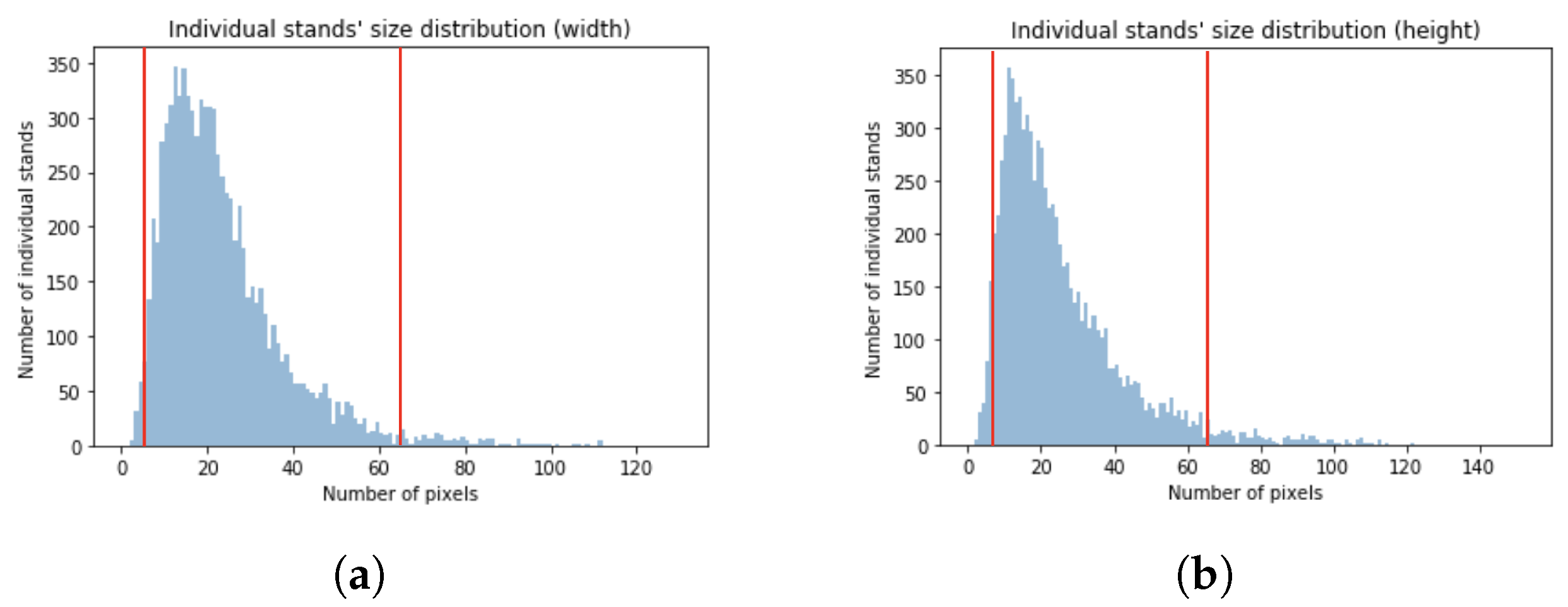
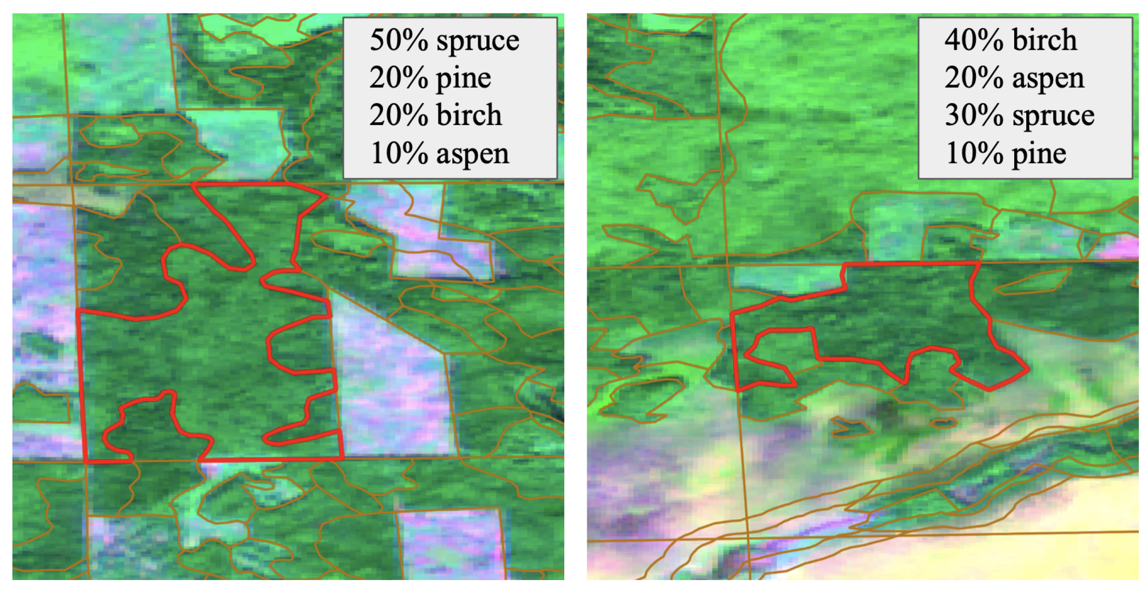
Another important issue is markup limitations. Field-based measurements are commonly used as reference data. Vast territories are often split into small aggregated areas comprised of groups of trees called individual stands [30]. These stands are not necessarily homogeneous but, in some cases, the percentages of different tree species within the stand is available [26]. The location of the non-dominant trees is unknown. In such cases, machine learning algorithms are often trained to predict the dominant class even for regions with mixed forest species [31], or just areas with a single dominant tree species are selected [32]. This raises the issue of weak markup adjustment. Among weakly supervision tasks, this one belongs to inexact supervision when only coarse-grained labels are given [33]. Weakly supervised images occur both in the general domain [34,35] and in specific tasks such as medical images segmentation [36]. These studies involve new neural network architectures or frameworks development to decrease requirements for labor-intensive data labeling. 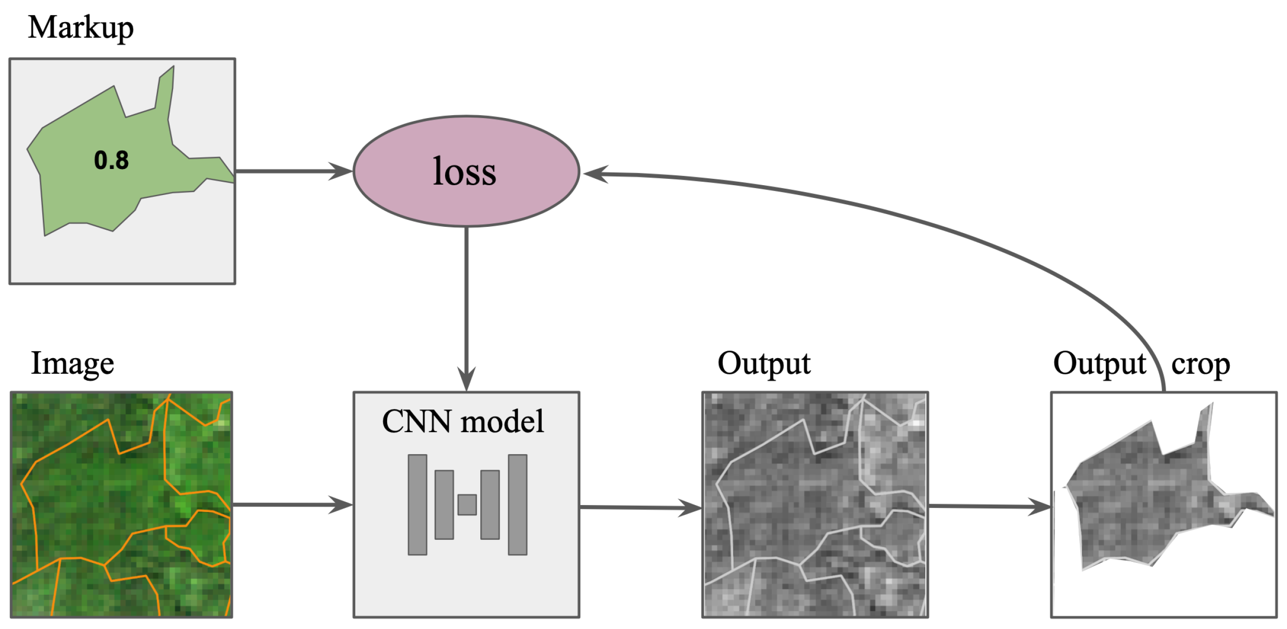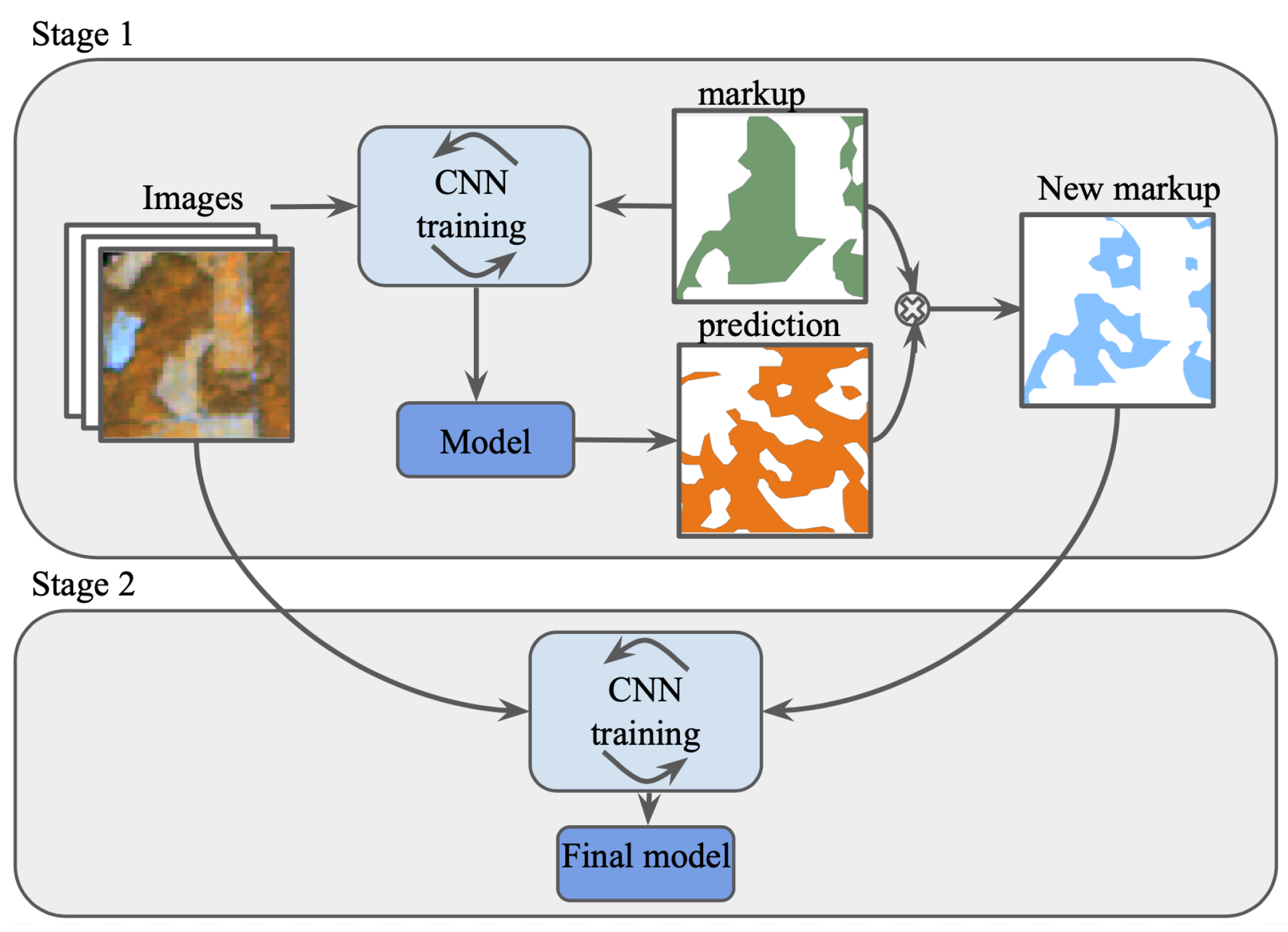In the remote sensing domain weakly supervised learning was also considered in different tasks such as cropland segmentation using low spatial resolution satellite data [37], cloud detection through high resolution images [38], and detection of red-attacked trees with very high resolution areal images [39]. However, in the field of forest species classification, the weak markup problem requires additional analysis according to data specificity (both satellite and field-based). In this study, we propose a CNN-based approach to extract more homogeneous areas from the traditional forest inventory data that includes only species’ content within stands and does not provide each species’ location. We focus on semantic segmentation problem using high resolution multispectral satellite data. The approach is particularly based on the Co-teaching paradigm presented in [40] where two neural networks are trained, and small-loss instances are selected as clean data for image classification task. In contrast, we split the data adjustment and training process into two separate stages and implement this pipeline for the semantic segmentation task.

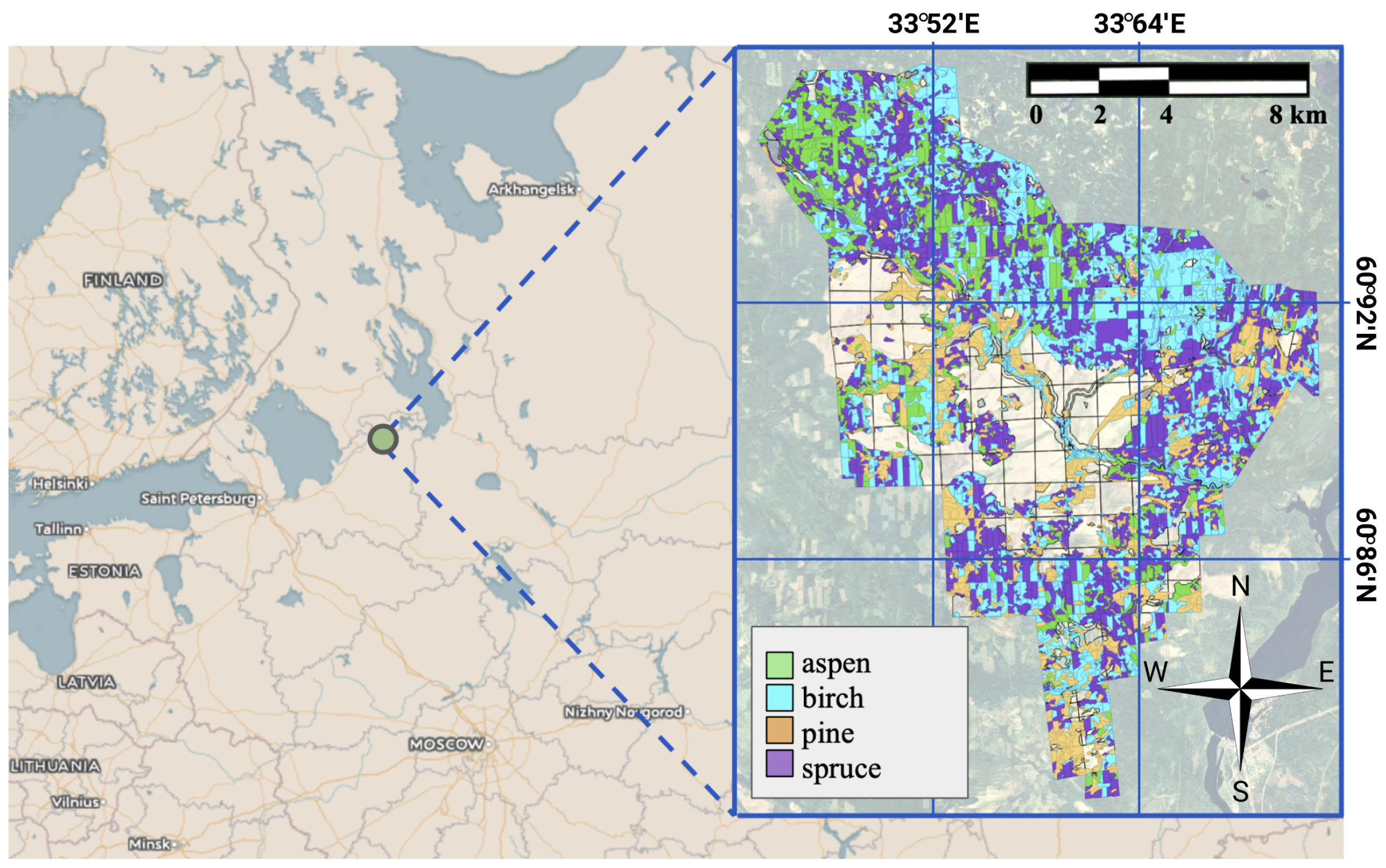
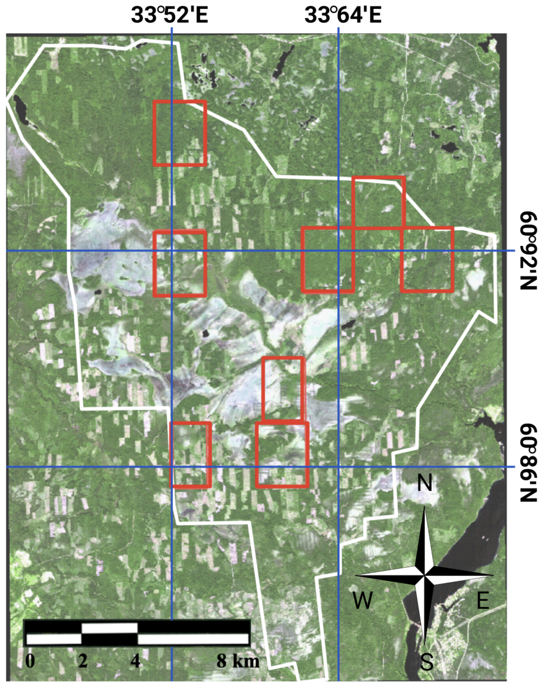
In this study, we aim to explore a deep neural network approach for forest type classification in Russian boreal forests using Sentinel-2 images. We set the following objectives:

• to develop a novel approach for forest species classification using convolutional neural networks (CNN) combining pixel- and object-wise approaches during the training procedure, and compare it with a typically used approach for semantic segmentation; and
• to provide a strategy for weak markup improvements and examine forest type classification both as a problem of (a) dominant class estimation for non-homogeneous individual stands and (b) more precise homogeneous classification.

2. Materials and methods

2.1. Study Site

The study was conducted in the Russian boreal forests of Leningrad Oblast. The coordinates of these regions are between ${33}^{\circ }{42}^{\prime }$ and ${33}^{\circ }{76}^{\prime }$ longitude and between ${60}^{\circ }{78}^{\prime }$ and ${61}^{\circ }{01}^{\prime }$ latitude (Figure 1). The vegetation cover is mixed and includes deciduous and conifer tree species. The main species are pine, spruce, aspen, and birch. The climate in the region is humid. An average daily high temperature in the vegetation period (from May to August) is above 15 °C. The rain period usually lasts for 7 months (from April to November). From September to May, it is snowy (or rain mixed with snow). Throughout the course of the year, the region is generally cloudy (with the clearer periods during the summer time, when the probability of a clear sky is about $20\%$) [41].

2.2. Reference Data

Reference data was previously reported in [26]. It was collected by field-based measurements carried out in July-August 2018. The methodology of data gathering corresponded to the official Russian inventory regulation [30]. In accordance, the study area was split into individual stands with the following characteristics: polygonal coordinates, a certain percentage of each tree species, average age, and height within the stand. The distribution of stand sizes is presented in Figure 2. The majority of polygons had their longest side length between 100 and 600 m. Although the percentage for each stand was defined, the spatial distribution within the stand was unknown. The number of individual stands with particular dominant tree species (larger than $50\%$ within the stand) is shown in Figure 3 and in

Table 1. Dataset statistics.

	Training	Test	All	Area (ha)
	Individual Stands	Individual Stands	Individual Stands
aspen	520	205	725	2298
birch	1143	501	1644	4165
pine	1569	726	2295	3620
spruce	1087	450	1537	6315

. The vast majority of individual stands consisted of mixed species; for instance, there were less than 100 stands of pure (not mixed) birch type. Example of mixed individual stands are presented in Figure 4.

2.3. Satellite Data

For optical multispectral imagery, we acquired Sentinel-2 data. This data is available for free download in L1C format from EarthExplorer USGS [42]. Tiles IDs and acquisition dates are presented in

Table 2. Sentinel-2 images from USGS. Wavelength values corresponding to each band: Band 2: Blue, 458–523 nm; Band 3: Green, 543–578 nm; Band 4: Red, 650–680 nm; Band 5: Red-edge I (R-edge I), 698–713 nm; Band 6: Red-edge II (R-edge II), 733–748 nm; Band 7: Red-edge III (R-edge III), 773–793 nm; Band 8: Near infrared (NIR), 785–900 nm; Band 8A: Narrow Near infrared (NNIR), 855–875 nm; Band 11: Shortwave infrared-1 (SWIR1), 1566–1651 nm; Band 12: Shortwave infrared-2 (SWIR2), 2100–2280 nm).

Tile ID	Date	Cloud	10 m	20 m	Level of
		Coverage	Bands	Bands	Processing
L1C_T36VWN_A010343_20170615T090713	2017.06.15	0	2, 3,	5, 6, 7,	L1C
			4, 8	8A, 11, 12
L1C_T36VWN_A016206_20180730T090554	2018.07.30	0	2, 3,	5, 6, 7,	L1C
			4, 8	8A, 11, 12

. In this study, we considered only summer images. High cloud cover imposes limits on data for this northern region. Therefore, only two summer images from different years but of the comparable summer period were used to create the training dataset. Images acquired in other summer dates did not provide a sufficient amount of clear areas without clouds. There were no significant forest cover changes between survey time and image acquisition time; therefore, both images are relevant for the study. 10 bands of the following wavelengths were used: Band 2: Blue, 458–523 nm; Band 3: Green, 543–578 nm; Band 4: Red, 650–680 nm; Band 5: Red-edge I (R-edge I), 698–713 nm; Band 6: Red-edge II (R-edge II), 733–748 nm; Band 7: Red-edge III (R-edge III), 773–793 nm; Band 8: Near infrared (NIR), 785–900 nm; Band 8A: Narrow Near infrared (NNIR), 855–875 nm; Band 11: Shortwave infrared-1 (SWIR1), 1566–1651 nm; Band 12: Shortwave infrared-2 (SWIR2), 2100–2280 nm). Images were pre-processed with the Sen2Cor package [43] for atmospheric correction. Although, Sen2Cor package provides a cloud and shadow map, which can be used to eliminate irrelevant pixels, we selected cloudless images for the study. The obtained data were in L2A format, including values of Bottom-Of-Atmosphere (BOA) reflectances. For CNN-based tasks, image values are often brought to the interval from 0 to 1 [44,45]. Therefore, pixel values were mapped to the interval $[0,1]$ through division by 10,000 (the maximum physical surface reflectance value for Sentinel-2 in level L2A) and clipping to 0 and 1. We used bands with a spatial resolution of 10 m per pixel ($B02,B03,B04,B08$ bands) and 20 m per pixel ($B05,B06,B07,B11,B12,B8A$ bands), adjusted to 10 m by Nearest Neighbor interpolation [46]. Each image covered the entire study area, and images were considered separately without any spatial averaging (the same as in [47]).

2.4. Organizing Samples for Classification

Four tree species were considered: aspen, birch, spruce, and pine. We also considered the ’conifer’ class as a combination of spruce and pine, and the ’deciduous’ class as a combination of aspen and birch. As a sample for the further analysis, we chose individual stands. There was no information on the spatial distribution of tree species within an individual stand. Therefore, we defined the label for each stand as the dominant tree species within it, if the stand contained more than $50\%$ of this forest type (the same approach was described in [31]). For conifer and deciduous classes, we summed the percentages for spruce and pine, and for aspen and birch, respectively. The described sample definition assumed that the markup had some pre-defined uncertainty for non-homogeneous stands. However, it provided information necessary to the dominant species classification task. Thus, for each sample in the data set, we know the label of the dominant forest type, the percentage of secondary types (if any), and an ascribed polygon in a multispectral satellite image.

For the experiment of training procedure adjustment, we selected 8 test regions of about 450 ha each (Figure 5). For the experiment of weak markup improvement, $30\%$ of samples were selected randomly for test. Samples outside test regions were split into train and validation sets randomly, in a ratio of 7:3, following the constraint of no occurrence of the same individual stand in both validation and training sets. For each polygon it can be more than one sample depending on the images’ number covering the polygon. Non-overlapping parts of the same satellite image could appear in both the training and test sets.

2.5. Forest Species Classification

Instead of typical multi-class classification, we used an hierarchical approach described in [26]. The task of four-species prediction was split into three tasks: (a) classification of conifer and deciduous; (b) classification of birch and aspen; and (c) classification of spruce and pine. The final results followed from the intersection between the predicted mask of birch and aspen and the predicted deciduous mask (with a similar approach followed in the conifer case). Such an hierarchical approach allows for solving each task independently and ensuring greater control over experiment at each step.

For the forest type classification, we implemented a deep neural network approach, which have been widely used for image classification and segmentation tasks when spatial characteristics are important in the remote sensing domain [48,49,50]. At the input of such a neural network, there is usually a combination of spectral bands. The output of the semantic segmentation model is a map, where each pixel is ascribed a particular class label. During the training procedure, a model is forced to correctly predict as many pixel labels as possible by observing random image patches with pre-defined size. This is achieved through the implementation of a particular loss function. The loss is computed for each step of neural network training, when all images patches from one batch have been processed. For our study, we implemented the categorical cross entropy per-pixel loss function:

$$\begin{array}{c}\hfill \mathrm{Loss}=-\frac{{\sum }_{i=1}^N{\sum }_{k=1}^C(y_{ik}\times log{\widehat{y}}_{ik})}{N},\end{array}$$

(1)

where ${\widehat{y}}_{ik}$—predicted probability of the ith pixel to belong to the kth class, $y_{ik}$—ground truth value for the ith pixel (1 if the pixel belongs to the kth class), N—number of not masked pixels, C—number of classes.

In this loss, all pixels in the scene are taken into account. Therefore, if the classes are highly unbalanced, a model rarely observes pixels labeled as the smaller class. This results in poor performance of the model for a less represented class. A common solution is using a larger penalty for errors on the smaller class samples, such as in the weighted categorical cross entropy:

$$\begin{array}{c}\hfill \mathrm{Weighted}\mathrm{Loss}=-\frac{{\sum }_{i=1}^N{\sum }_{k=1}^C(y_{ik}\times log{\widehat{y}}_{ik})\times weights\left(y_{ik}\right)}{N},\end{array}$$

(2)

where ${\widehat{y}}_{ik}$—predicted probability of the ith pixel to belong to the kth class, $y_{ik}$—ground truth value for the ith pixel (1 if the pixel belongs to the kth class), N—number of not masked pixels, C—number of classes.

Another issue that should be taken into account is that samples of particular classes may not be evenly distributed across the study region. This means that random selection of image patches in batch can lead to a situation where samples concentrated in one area may be seldom observed.

To tackle this problem, we modified the classical sampling approach for semantic segmentation with CNN, as described in the next section.

2.6. Object-Wise Sampling Approach

We replaced the commonly used batch creation approach. The sample content was taken into account, instead of simply using random patch selection. The choice of patch size was governed by the relevant size of polygons. As we eliminated polygons with sides less than 80 m and larger than 640 m, the patch size was selected as $64\times 64$ pixels. The number of patches per batch was set to 128. Although we considered two classes, the general approach is also applicable for more classes. For each class, we picked the same number of polygons and cut patches around these polygons to create the batch. As the polygon size could vary in the defined range, the patch crop could also differ for the same polygon. The only demand was that the polygon’s bounding box should be within the patch boundary. The patch was also geometrically augmented, in order to provide more variability during the training procedure. We implemented random rotate, mirror, and flip operations. The general approach for batch creation is described in Algorithm 1.

Algorithm 1: Batch Creation

The next step was loss computation. The approach is described in the Figure 6. For this purpose, we used polygon mask. Patch has dimension $Patch\_Rows,Patch\_Columns$, $Number\_of\_classes$. The patch mask contains non-zero values for pixels within the polygon’s area and for the appropriate correct class. Despite the fact that individual stands are not often homogeneous, all pixels within one stand were ascribed the same label. The loss was computed for this area. There can be an available markup for other pixels within the patch, but this was not considered. The main reason for this is that it can affect the balance of classes.

We compared this approach with the commonly used per-pixel semantic segmentation approach, for which the batch was randomly formed and an extra penalty for mistakes in the smaller class was added (Figure 7). In this approach, for calculation of the weighted categorical cross-entropy loss, all pixels within the patch were considered. The weights were set proportionally to the amount of each class represented.

2.7. Weak Markup

Another adjustment was aimed at addressing weak markup. It includes two stages, as shown in the Figure 8. The first stage was as follows. The aforementioned reference data consisted of the percentage of each class within the individual stand. We took this knowledge during the loss computation. The loss was calculated for each individual stand and multiplied by the dominant species percentage. For example, for a stand that consisted $60\%$ of conifers and $40\%$ of deciduous trees, the penalty will be $0.6$. If the percentage is higher, then the penalty becomes stricter. For a homogeneous stand, all pixels have the maximum loss weights. Therefore, in Equation (2), weights were defined as the dominant species percentage. When the learning curve started to change less rapidly and could achieve sufficient results on the validation set (after about 15 epochs), we changed the training data set. We eliminated all individual stands with percentage less than $90\%$. Thus, for a few epochs (about 2 epochs), the model observes more pure data. Obviously, such a model will perform poorly, in terms of the initial dominant species problem statement. However, at the same time, it will not strive to label deciduous trees within a conifer individual stand as conifer trees (as for case with $60\%$ conifer and $40\%$ deciduous). Then, we used this model to predict conifer and deciduous species both for training and validation regions. The first stage of markup adjustment results was the intersection between the predicted mask and initial dominant species markup. It was assumed that the map acquired in this way contained less pixels of minor (i.e., non-dominant) classes.

The next stage of the weak markup study was the implementation of the newly obtained markup in further training. We intersected the new conifer mask with the initial spruce and pine dominant masks, and the same for the deciduous classes. The goal of this intersection was to reduce the number of deciduous pixels within individual stands dominated by pine and spruce, and vice versa. For this study, we created the validation data set only from homogeneous individual stands.

2.8. Experimental Setup

For all experiments, the U-Net architecture [51] with ResNet [52] encoder was used, as it has been shown to successfully perform in popular image classification tasks both in general and remote sensing domains [50]. The model implementation referred to [53]. It used Keras [54] with Tensorflow [55] backend. For model training, a PC with GTX-1080Ti GPUs was used. The batch size was 128 patches, where each patch had size of $64\times 64$ pixels. The batch size was chosen accord-ing to GPU memory limitations. There were 100–200 steps per epoch and the number of epochs varied from 10 to 30, depending on the size of classes. Similar results reproduction was achieved by fixing a random seed for pseudo-random number generator for all training methods.

2.9. Validation Methods

To assess the classification quality, we considered F1-score (Equation (5)). It is a commonly used score for semantic segmentation tasks [56], in particular in cases of unbalanced datasets. F1-score is also often considered in the remote sensing domain [50].

$$\begin{array}{c}\hfill P=\frac{TP}{TP+FP}\end{array}$$

(3)

$$\begin{array}{c}\hfill R=\frac{TP}{TP+FN}\end{array}$$

(4)

$$\begin{array}{c}\hfill F1=\frac{2\times P\times R}{P+R}\end{array}$$

(5)

where P is precision, R is recall, $TP$ is True Positive (the number of correctly classified pixels/stands of a given class), $FP$ is False Positive (the number of pixels/stands classified as a given class while being of another class), and $FN$ is False Negative (the number of pixels/stands of a given class missed by the model).

In the one case, we evaluated the number of correctly predicted individual stands. To this end, per-pixel predictions within stands were aggregated and the dominant class was defined for each stand. Based on reference and predicted stand labels, the amounts of true positive, false positive, and false negative samples were estimated. In the second case, we evaluated the F1-score in a per-pixel manner.

A CNN model for each experiment was trained five times with different random seeds, and then results were averaged. Standard deviation was computed.

3. Results

3.1. Sampling Approach for Species Classification

We compared a typical sampling procedure for forest species semantic segmentation with our modified one. The results are presented in

Table 3. Forest types classification using different sampling procedure (per-pixel F1-score).

	Aspen/Birch	Pine/Spruce	Conifer/Deciduous	Average
Simple sampling procedure	0.48/0.88	0.91/0.88	0.81/0.85	0.8 ± 0.003
Modified sampling procedure	0.63/0.91	0.94/0.88	0.85/0.87	0.85 ± 0.004

. For all classes, the object-wise sampling approach performed better. The average F1-score before aggregation was improved from $0.8$ to $0.85$. The final aggregated results were obtained by multiplying the predicted conifer binary mask with spruce and pine masks and multiplying the predicted deciduous mask with aspen and birch masks. Aggregated results for four forest classes are shown in Table 6. The object-wise sampling approach allows us to improve segmentation’s F1-score from $0.68$ to $0.74$. The larger difference between the two methods was for the birch and aspen classes. The reason for this is that these classes were the most difficult to distinguish due to imbalance. The proposed approach leads to a more balanced training samples choice.

Standard deviation was computed for averaged F1-score of different model training running. It shows that achieved results are relevant for further forest analysis studies.

3.2. Markup Adjustment

We conducted experiments aimed to improve conifer and deciduous markup. Some areas were eliminated by the model predictions intersected with the initial dominant species map. It aims to leave only homogeneous areas with conifer or deciduous trees. The per-pixel metric is intended to label all pixels even within inhomogeneous individual stand as the dominant class type. Therefore, at this stage of the task, the goal was not to improve the per-pixel score. The average per-pixel F1-score for conifer and deciduous classification became $0.76$, in comparison with the previously achieved $0.82$ (

Table 4. Conifer and deciduous classification (average score) using source markup and updated markup.

	Per-Pixel F1-Score	Per-Stand F1-Score
Source markup	0.827	0.851
Updated markup	0.769	0.854

). However, we aimed to preserve the score per individual stands than the per-pixel one. The score of dominant classification per individual stands was still approximately at the same level (F1-score $0.85$). It means that the model was trained to ignore pixels of non-dominant classes within the stand. For the further assessment, homogeneous stands were considered.

The obtained map was then used for species classification. We compared the model trained on the source markup and that trained on updated one. Their performances were assessed on homogeneous individual stands for four species from the test set. The results are presented in

Table 5. Forest types classification for more homogeneous individual stands (per-pixel F1-metric) using source markup and updated markup. Results on test samples.

	Aspen/Birch	Pine/Spruce	Average
Source markup	0.77/0.9	0.94/0.88	0.87 ± 0.003
Updated markup	0.79/0.91	0.95/0.9	0.89 ± 0.002

. Although we eliminated pixels from the (non-homogeneous) training set, the model performed better than when using the larger training data of weaker quality. It allowed us to improve the average F1-score for four species from $0.74$ to $0.76$ compared with initial markup usage (

Table 6. Final aggregated results for forest types classification using modified sampling procedure and markup adjustment (F1-score).

	Aspen	Birch	Pine	Spruce	Average
Simple sampling procedure	0.42	0.72	0.84	0.74	0.68 ± 0.007
Modified sampling procedure	0.6	0.8	0.81	0.74	0.74 ± 0.004
Modified sampling procedure with new markup	0.62	0.83	0.82	0.76	0.76 ± 0.005

). The results confirmed the benefit of the proposed approach.

Example of the final predictions using both modified sampling approach and adjusted markup is presented in Figure 9.

4. Discussion

4.1. Sampling Approach for Species Classification

The analysis showed that the sampling procedure is highly essential for the forest species classification task. The same approach can be implemented for other problems where maps of vast territories are used and some classes are distributed not uniformly. The proposed object-wise sampling approach for CNN leads to better results than the commonly used approach where patches are chosen randomly within the entire satellite image.

It is worth mentioning the reason why a classical patch-wise approach was not considered suitable for our problem. It implies that we can choose the patch size small enough to include just the pixels of one class. However, in our case, there are two obstacles to implement this. The first being that individual stands are not of rectangular shape and, therefore, the patch size must be rather small. The other point is that individual stands are not homogeneous and we do not know the spatial distributions within stands. Therefore, a random small patch within an individual stand may turn out to, in fact, be a set of pixels of a minor class. This makes the approach described in [21] inappropriate in the presented case.

Another alternative approach to classical pixel- and object-wise classification for remote sensing applications (e.g., airplane-based) has been discussed in [25]. It should be noted that, despite the apparent similarity of airplane and satellite-derived remote sensing data, they have substantive differences. The main difference is spatial resolution. The relevant observation field can vary by 100 times (e.g., $0.1$ m for UAV and 10 m for satellite images). Thus, the approach have to be modified.

4.2. Markup Adjustment

Clear markup is essential for remote sensing tasks. In some cases, non-homogeneous areas are excluded from training set [32]. Another approach is to use plots with different species and ascribed it by the dominant species class [31]. It is reasonable to move further in the direction of an automatic markup adjustment, in order to make the data clearer without extra manual labeling. The next step of the study can be label adjustment for all classes, not only for conifer and deciduous. The weighted loss function adjustment can also be considered to improve homogeneous areas detection.

Weakly supervised learning is now applied in different remote sensing tasks. They vary by the target objects and remote sensing data properties such as spatial resolution and spectral bands number. In our study, we focus on 10 m spatial resolution and 10 multispectral bands. In cases of very high spatial resolution and just RGB bands such as in [39] markup constraints differ significantly. Particular tasks also pose some limitations and additional opportunities for a weakly supervised learning approach [38]. Therefore, remote sensing datasets can differ drastically from such datasets as MNIST or CIFAR considered in [40]. Another difference is that the forest species classification is considered as a semantic segmentation task instead of an image classification task, such as in the case of noisy labels problem in [40].

Markup adjustment can be also studied in the case with machine learning algorithms instead of neural network based such as methods described in [57,58,59].

The main error source in such land cover tasks is diversity within each forest species. Spectral characteristics vary drastically for different tree age and depend on environmental conditions. Therefore, markup adjustment and optimal sampling choice are promising approaches to improve model performance. Another error source is mixed border pixels of neighboring individual stands. In the case of 10 m spatial resolution, even for homogeneous forest stands, spectral characteristics on the border can be affected by other species outside this stand. A possible approach to address this problem for homogeneous stands is to consider just inner pixels remote from the border.

One of the potential limitations is the time and computational cost for markup adjustment model training. In our case, we used the same CNN architecture to perform this stage. We trained the model for markup adjustment and the final segmentation model sequentially. In future studies, an alternative approach can be developed and implemented to perform markup adjustment on the fly for remote sensing tasks.

In this study, we considered forest species classification. However, the proposed approach can be transferred in future studies for other tasks where samples are grouped, and for a group, label distribution is known. The described approach is also applicable for other neural network architectures. Therefore, experiments with new state-of-the-art architectures can be conducted using the same method. Both the sampling and markup adjustment approaches are transferable to new satellite data sources. We considered multispectral Sentinel-2 imagery with a spatial resolution of 10 m. However, it can also be implemented for high-resolution multispectral data such as WorldView or just RGB images such as base maps.

Vegetation indices are significant for environmental tasks as they provide relevant surface characteristics. Therefore, they are widely used as features for classical machine learning methods. However, in the case of deep neural networks, it is assumed that neural networks can learn non-linear connections between raw input data and use prior information for more general characteristics extraction. In our study, we considered only multispectral satellite bands. However, future studies might include vegetation indices or supplementary materials such as digital elevation or canopy height models to achieve higher results and reduce training time.

It is promising to study different augmentation techniques combined with improved markup and the object-wise sampling approach. For example, the object-based augmentation described in [60] can further be implemented to create more variable training samples with different homogeneous stands.

Precise forest species classification can also be implemented in ecological and environmental studies, as large forest patches have been proved to affect human health [61]. Detailed forest characteristics can be helpful for such analysis.

5. Conclusions

The sampling approach and ground truth markup quality are crucial in forestry tasks involving remote sensing data. In this study, we analyzed the potential of combining CNN and Sentinel-2 images for the task of forest species classification using weak markup with non-homogeneous individual stands. During the first stage, a CNN was trained to find the homogeneous areas within each stand, providing a more accurate markup. During the second stage, the final model was trained to predict four forest species. This markup adjustment allows us to increase F1-score from $0.74$ to $0.76$ compared to the initial markup. The experiment confirms the opportunity of finding weak labels and shows promising results for further classification enhancement. We also proposed the CNN-based sampling approach for spatial data in forest species classification. The proposed modification outperformed the prediction quality of a commonly used per-pixel semantic segmentation model (the average F1-metric was increased from $0.68$ to $0.74$). The described pipeline helps to address the issue of highly imbalanced and not evenly distributed classes. The provided training strategy can help solve forest species classification tasks more precisely, even when the reference data has significant limitations. Further study for other vast territories is promising, and the proposed sampling technique seems to be beneficial in such spatial studies.

References

1. Lindenmayer, D.B.; Margules, C.R.; Botkin, D.B. Indicators of biodiversity for ecologically sustainable forest management. Conserv. Biol. 2000, 14, 941–950. [Google Scholar] [CrossRef]
2. Franklin, J.; Andrade, R.; Daniels, M.L.; Fairbairn, P.; Fandino, M.C.; Gillespie, T.W.; González, G.; Gonzalez, O.; Imbert, D.; Kapos, V.; et al. Geographical ecology of dry forest tree communities in the West Indies. J. Biogeogr. 2018, 45, 1168–1181. [Google Scholar] [CrossRef] [Green Version]
3. Wallace, K.J.; Clarkson, B.D. Urban forest restoration ecology: A review from Hamilton, New Zealand. J. R. Soc. N. Z. 2019, 49, 347–369. [Google Scholar] [CrossRef]
4. Hill, A.; Buddenbaum, H.; Mandallaz, D. Combining canopy height and tree species map information for large-scale timber volume estimations under strong heterogeneity of auxiliary data and variable sample plot sizes. Eur. J. For. Res. 2018, 137, 489–505. [Google Scholar] [CrossRef] [Green Version]
5. Bont, L.G.; Hill, A.; Waser, L.T.; Bürgi, A.; Ginzler, C.; Blattert, C. Airborne-laser-scanning-derived auxiliary information discriminating between broadleaf and conifer trees improves the accuracy of models for predicting timber volume in mixed and heterogeneously structured forests. For. Ecol. Manag. 2020, 459, 117856. [Google Scholar] [CrossRef]
6. Pandey, P.C.; Anand, A.; Srivastava, P.K. Spatial distribution of mangrove forest species and biomass assessment using field inventory and earth observation hyperspectral data. Biodivers. Conserv. 2019, 28, 2143–2162. [Google Scholar] [CrossRef]
7. Persson, H.J.; Olsson, H.; Soja, M.J.; Ulander, L.M.; Fransson, J.E. Experiences from large-scale forest mapping of Sweden using TanDEM-X data. Remote Sens. 2017, 9, 1253. [Google Scholar] [CrossRef] [Green Version]
8. Lei, Y.; Siqueira, P.; Chowdhury, D.; Torbick, N. Generation of large-scale forest height mosaic and forest disturbance map through the combination of spaceborne repeat-pass InSAR coherence and airborne lidar. In Proceedings of the 2016 IEEE International Geoscience and Remote Sensing Symposium (IGARSS), Beijing, China, 10–15 July 2016; pp. 5342–5345. [Google Scholar]
9. Pasquarella, V.J.; Holden, C.E.; Woodcock, C.E. Improved mapping of forest type using spectral-temporal Landsat features. Remote Sens. Environ. 2018, 210, 193–207. [Google Scholar] [CrossRef]
10. Gudex-Cross, D.; Pontius, J.; Adams, A. Enhanced forest cover mapping using spectral unmixing and object-based classification of multi-temporal Landsat imagery. Remote Sens. Environ. 2017, 196, 193–204. [Google Scholar] [CrossRef]
11. Stoian, A.; Poulain, V.; Inglada, J.; Poughon, V.; Derksen, D. Land cover maps production with high resolution satellite image time series and convolutional neural networks: Adaptations and limits for operational systems. Remote Sens. 2019, 11, 1986. [Google Scholar] [CrossRef] [Green Version]
12. Nguyen, T.H.; Jones, S.D.; Soto-Berelov, M.; Haywood, A.; Hislop, S. A spatial and temporal analysis of forest dynamics using Landsat time-series. Remote Sens. Environ. 2018, 217, 461–475. [Google Scholar] [CrossRef]
13. Campos-Taberner, M.; García-Haro, F.J.; Martínez, B.; Izquierdo-Verdiguier, E.; Atzberger, C.; Camps-Valls, G.; Gilabert, M.A. Understanding deep learning in land use classification based on Sentinel-2 time series. Sci. Rep. 2020, 10, 1–12. [Google Scholar] [CrossRef] [PubMed]
14. Illarionova, S.; Nesteruk, S.; Shadrin, D.; Ignatiev, V.; Pukalchik, M.; Oseledets, I. MixChannel: Advanced Augmentation for Multispectral Satellite Images. Remote Sens. 2021, 13, 2181. [Google Scholar] [CrossRef]
15. Eo-Learn. 2020. Available online: https://github.com/sentinel-hub/eo-learn (accessed on 20 August 2020).
16. Breiman, L. Random forests. Mach. Learn. 2001, 45, 5–32. [Google Scholar] [CrossRef] [Green Version]
17. Cortes, C.; Vapnik, V. Support-vector networks. Mach. Learn. 1995, 20, 273–297. [Google Scholar] [CrossRef]
18. Hamedianfar, A.; Barakat, A.; Gibril, M. Large-scale urban mapping using integrated geographic object-based image analysis and artificial bee colony optimization from worldview-3 data. Int. J. Remote Sens. 2019, 40, 6796–6821. [Google Scholar] [CrossRef]
19. Chen, Y.; Zhou, Y.; Ge, Y.; An, R.; Chen, Y. Enhancing land cover mapping through integration of pixel-based and object-based classifications from remotely sensed imagery. Remote Sens. 2018, 10, 77. [Google Scholar] [CrossRef] [Green Version]
20. Kussul, N.; Shelestov, A.; Lavreniuk, M.; Butko, I.; Skakun, S. Deep learning approach for large scale land cover mapping based on remote sensing data fusion. In Proceedings of the 2016 IEEE International Geoscience and Remote Sensing Symposium (IGARSS), Beijing, China, 10–15 July 2016; pp. 198–201. [Google Scholar]
21. Mahdianpari, M.; Salehi, B.; Rezaee, M.; Mohammadimanesh, F.; Zhang, Y. Very deep convolutional neural networks for complex land cover mapping using multispectral remote sensing imagery. Remote Sens. 2018, 10, 1119. [Google Scholar] [CrossRef] [Green Version]
22. Illarionova, S.; Shadrin, D.; Trekin, A.; Ignatiev, V.; Oseledets, I. Generation of the NIR spectral Band for Satellite Images with Convolutional Neural Networks. Sensors 2021, 21, 5646. [Google Scholar] [CrossRef]
23. DeLancey, E.R.; Simms, J.F.; Mahdianpari, M.; Brisco, B.; Mahoney, C.; Kariyeva, J. Comparing deep learning and shallow learning for large-scale wetland classification in Alberta, Canada. Remote Sens. 2020, 12, 2. [Google Scholar] [CrossRef] [Green Version]
24. Chen, T.; Guestrin, C. Xgboost: A scalable tree boosting system. In Proceedings of the 22nd ACM Sigkdd International Conference On Knowledge Discovery and Data Mining, San Francisco, CA, USA, 13–17 August 2016; pp. 785–794. [Google Scholar]
25. Sun, Y.; Huang, J.; Ao, Z.; Lao, D.; Xin, Q. Deep Learning Approaches for the Mapping of Tree Species Diversity in a Tropical Wetland Using Airborne LiDAR and High-Spatial-Resolution Remote Sensing Images. Forests 2019, 10, 1047. [Google Scholar] [CrossRef] [Green Version]
26. Illarionova, S.; Trekin, A.; Ignatiev, V.; Oseledets, I. Neural-Based Hierarchical Approach for Detailed Dominant Forest Species Classification by Multispectral Satellite Imagery. IEEE J. Sel. Top. Appl. Earth Obs. Remote Sens. 2020, 14, 1810–1820. [Google Scholar] [CrossRef]
27. Xia, G.S.; Bai, X.; Ding, J.; Zhu, Z.; Belongie, S.; Luo, J.; Datcu, M.; Pelillo, M.; Zhang, L. DOTA: A large-scale dataset for object detection in aerial images. In Proceedings of the IEEE Conference on Computer Vision and Pattern Recognition, Salt Lake City, UT, USA, 18–22 June 2018; pp. 3974–3983. [Google Scholar]
28. Xu, G.; Zhu, X.; Tapper, N. Using convolutional neural networks incorporating hierarchical active learning for target-searching in large-scale remote sensing images. Int. J. Remote Sens. 2020, 41, 4057–4079. [Google Scholar] [CrossRef]
29. Trisasongko, B.H.; Panuju, D.R.; Paull, D.J.; Jia, X.; Griffin, A.L. Comparing six pixel-wise classifiers for tropical rural land cover mapping using four forms of fully polarimetric SAR data. Int. J. Remote Sens. 2017, 38, 3274–3293. [Google Scholar] [CrossRef]
30. Order of the Federal Forestry Agency (Rosleskhoz) of 12 December 2011 N 516 Moscow “On approval of the Forest Inventory Instruction” Prikaz Federal’nogo Agentstva Lesnogo Hozyajstva (Rosleskhoz) ot 12 Dekabrya 2011 g. N 516 g. Moskva “Ob Utverzhdenii Lesoustroitel’noj Instrukcii”. Available online: https://rulaws.ru/acts/Prikaz-Rosleshoza-ot-12.12.2011-N-516/ (accessed on 20 August 2020).
31. Abdollahnejad, A.; Panagiotidis, D.; Shataee Joybari, S.; Surovỳ, P. Prediction of dominant forest tree species using quickbird and environmental data. Forests 2017, 8, 42. [Google Scholar] [CrossRef]
32. Knauer, U.; von Rekowski, C.S.; Stecklina, M.; Krokotsch, T.; Pham Minh, T.; Hauffe, V.; Kilias, D.; Ehrhardt, I.; Sagischewski, H.; Chmara, S.; et al. Tree species classification based on hybrid ensembles of a convolutional neural network (CNN) and random forest classifiers. Remote Sens. 2019, 11, 2788. [Google Scholar] [CrossRef] [Green Version]
33. Zhou, Z.H. A brief introduction to weakly supervised learning. Natl. Sci. Rev. 2017, 5, 44–53. [Google Scholar] [CrossRef] [Green Version]
34. Guo, S.; Huang, W.; Zhang, H.; Zhuang, C.; Dong, D.; Scott, M.R.; Huang, D. CurriculumNet: Weakly Supervised Learning from Large-Scale Web Images. In Proceedings of the European Conference on Computer Vision (ECCV), Munich, Germany, 8–14 September 2018. [Google Scholar]
35. Ahn, J.; Cho, S.; Kwak, S. Weakly Supervised Learning of Instance Segmentation With Inter-Pixel Relations. In Proceedings of the IEEE/CVF Conference on Computer Vision and Pattern Recognition (CVPR), Long Beach, CA, USA, 16–20 June 2019. [Google Scholar]
36. Xu, G.; Song, Z.; Sun, Z.; Ku, C.; Yang, Z.; Liu, C.; Wang, S.; Ma, J.; Xu, W. CAMEL: A Weakly Supervised Learning Framework for Histopathology Image Segmentation. In Proceedings of the IEEE/CVF International Conference on Computer Vision (ICCV), Seoul, Korea, 27–28 October 2019. [Google Scholar]
37. Wang, S.; Chen, W.; Xie, S.M.; Azzari, G.; Lobell, D.B. Weakly Supervised Deep Learning for Segmentation of Remote Sensing Imagery. Remote Sens. 2020, 12, 207. [Google Scholar] [CrossRef] [Green Version]
38. Li, Y.; Chen, W.; Zhang, Y.; Tao, C.; Xiao, R.; Tan, Y. Accurate cloud detection in high-resolution remote sensing imagery by weakly supervised deep learning. Remote Sens. Environ. 2020, 250, 112045. [Google Scholar] [CrossRef]
39. Qiao, R.; Ghodsi, A.; Wu, H.; Chang, Y.; Wang, C. Simple weakly supervised deep learning pipeline for detecting individual red-attacked trees in VHR remote sensing images. Remote Sens. Lett. 2020, 11, 650–658. [Google Scholar] [CrossRef]
40. Han, B.; Yao, Q.; Yu, X.; Niu, G.; Xu, M.; Hu, W.; Tsang, I.; Sugiyama, M. Co-teaching: Robust training of deep neural networks with extremely noisy labels. arXiv 2018, arXiv:1804.06872. [Google Scholar]
41. Weather Spark. 2020. Available online: https://weatherspark.com/ (accessed on 20 August 2020).
42. EarthExplorer USGS. Available online: https://earthexplorer.usgs.gov/ (accessed on 12 August 2020).
43. Sen2Cor. Available online: https://step.esa.int/main/third-party-plugins-2/sen2cor/ (accessed on 12 August 2020).
44. Vaddi, R.; Manoharan, P. Hyperspectral image classification using CNN with spectral and spatial features integration. Infrared Phys. Technol. 2020, 107, 103296. [Google Scholar] [CrossRef]
45. Debella-Gilo, M.; Gjertsen, A.K. Mapping Seasonal Agricultural Land Use Types Using Deep Learning on Sentinel-2 Image Time Series. Remote Sens. 2021, 13, 289. [Google Scholar] [CrossRef]
46. Persson, M.; Lindberg, E.; Reese, H. Tree species classification with multi-temporal Sentinel-2 data. Remote Sens. 2018, 10, 1794. [Google Scholar] [CrossRef] [Green Version]
47. Astola, H.; Häme, T.; Sirro, L.; Molinier, M.; Kilpi, J. Comparison of Sentinel-2 and Landsat 8 imagery for forest variable prediction in boreal region. Remote Sens. Environ. 2019, 223, 257–273. [Google Scholar] [CrossRef]
48. Zhang, W.; Tang, P.; Zhao, L. Remote sensing image scene classification using CNN-CapsNet. Remote Sens. 2019, 11, 494. [Google Scholar] [CrossRef] [Green Version]
49. Song, J.; Gao, S.; Zhu, Y.; Ma, C. A survey of remote sensing image classification based on CNNs. Big Earth Data 2019, 3, 232–254. [Google Scholar] [CrossRef]
50. Kattenborn, T.; Leitloff, J.; Schiefer, F.; Hinz, S. Review on Convolutional Neural Networks (CNN) in vegetation remote sensing. ISPRS J. Photogramm. Remote Sens. 2021, 173, 24–49. [Google Scholar] [CrossRef]
51. Ronneberger, O.; Fischer, P.; Brox, T. U-net: Convolutional networks for biomedical image segmentation. In Proceedings of the International Conference on Medical Image Computing And Computer-Assisted Intervention, Munich, Germany, 5–9 October 2015; pp. 234–241. [Google Scholar]
52. He, K.; Zhang, X.; Ren, S.; Sun, J. Deep residual learning for image recognition. In Proceedings of the IEEE Conference on Computer Vision and Pattern Recognition, Las Vegas, NV, USA, 27–30 June 2016; pp. 770–778. [Google Scholar]
53. Yakubovskiy, P. Segmentation Models. 2019. Available online: https://github.com/qubvel/segmentation_models (accessed on 20 August 2020).
54. Keras. 2019–2020. Available online: https://keras.io/ (accessed on 20 August 2020).
55. TensorFlow. 2019–2020. Available online: https://github.com/tensorflow/tensorflow (accessed on 20 August 2020).
56. Csurka, G.; Larlus, D.; Perronnin, F.; Meylan, F. What is a good evaluation measure for semantic segmentation? In Proceedings of the British Machine Vision Conference BMVC, Bristol, UK, 9–13 September 2013; Volume 27, pp. 10–5244. [Google Scholar]
57. Xia, J.; Yokoya, N.; Pham, T.D. Probabilistic mangrove species mapping with multiple-source remote-sensing datasets using label distribution learning in Xuan Thuy National Park, Vietnam. Remote Sens. 2020, 12, 3834. [Google Scholar] [CrossRef]
58. Ha, N.T.; Manley-Harris, M.; Pham, T.D.; Hawes, I. A comparative assessment of ensemble-based machine learning and maximum likelihood methods for mapping seagrass using sentinel-2 imagery in Tauranga Harbor, New Zealand. Remote Sens. 2020, 12, 355. [Google Scholar] [CrossRef] [Green Version]
59. Pham, T.D.; Bui, D.T.; Yoshino, K.; Le, N.N. Optimized rule-based logistic model tree algorithm for mapping mangrove species using ALOS PALSAR imagery and GIS in the tropical region. Environ. Earth Sci. 2018, 77, 1–13. [Google Scholar] [CrossRef]
60. Illarionova, S.; Nesteruk, S.; Shadrin, D.; Ignatiev, V.; Pukalchik, M.; Oseledets, I. Object-Based Augmentation Improves Quality of Remote Sensing Semantic Segmentation. arXiv 2021, arXiv:2105.05516. [Google Scholar]
61. Kim, J.; Park, D.B.; Seo, J.I. Exploring the Relationship between Forest Structure and Health. Forests 2020, 11, 1264. [Google Scholar] [CrossRef]
Figure 1. Region of interest. Enhanced RGB bands of Sentinel-2 image (tile id is L2A_T36VWN_A010343_20170615T090713) are shown.
Forests 12 01413 g001
Figure 2. Size distribution of individual stands within the study area. Polygons with a side larger than 64 pixels or smaller than 8 pixels were eliminated.
Forests 12 01413 g002
Figure 3. Distribution of classes.
Forests 12 01413 g003
Figure 4. Composite of B12, B08, B04 Sentinel-2 bands (tile id is L2A_T36VWN_A010343_20170615T090713). Example of mixed individual stands (red polygon) with percentages of species.
Forests 12 01413 g004
Figure 5. The whole study area (white polygon). Test regions (red polygons). Enhanced RGB bands of Sentinel-2 image (tile id is L2A_T36VWN_A010343_20170615T090713) are shown.
Forests 12 01413 g005
Figure 6. The object-wise semantic segmentation approach. The model produces the map where the probability of a class is recorded at each pixel. Loss is computed just for masked area of the polygon. The percentage of dominant class is also can be taken into consideration (in the example, the dominant species percentage for the individual stand is 0.8 ).
Forests 12 01413 g006
Figure 7. The commonly used per-pixel semantic segmentation approach. The model produces the map where the probability of a class is recorded at each pixel. Loss is computed for the entire patch. The patch includes stands with different dominant species (class 0, class 1, etc.).
Forests 12 01413 g007
Figure 8. Markup adjustment strategy.
Forests 12 01413 g008
Figure 9. Sentinel-2 RGB image (tile id is L2A_T36VWN_A010343_20170615T090713). Final predictions using modified sampling approach and adjustment markup.
Forests 12 01413 g009