
Lean Pattern in an Altitude Range Shift of a Tree Species: Abies pinsapo Boiss.
by
 , , and
Antonio González-Hernández
1,† ,
,
Diego Nieto-Lugilde
2,
Julio Peñas
1 and
Francisca Alba-Sánchez
1,* 1
Department of Botany, University of Granada. C.U. Fuentenueva, 18071 Granada, Spain
2
Department of Botany, Ecology and Plant Physiology, University of Cordoba, C.U. Rabanales, 14014 Córdoba, Spain
*
Author to whom correspondence should be addressed.
†
This work was part of the Doctor thesis of the first author Antonio González-Hernández. Doctor program in University of Granada, Granada, Spain.
Forests 2021, 12(11), 1451; https://0-doi-org.brum.beds.ac.uk/10.3390/f12111451
Submission received: 18 September 2021
/
Revised: 18 October 2021
/
Accepted: 21 October 2021
/
Published: 25 October 2021
(This article belongs to the Special Issue Past Environmental Changes and Forest Conservation)
Abstract
:Organisms modify their geographical distributions in response to changes in environmental conditions, or modify their affinity to such conditions, to avoid extinction. This study explored the altitudinal shift of Abies pinsapo Boiss. in the Baetic System. We analysed the potential distribution of the realised and reproductive niches of A. pinsapo populations in the Ronda Mountains (Southern Spain) by using species distribution models (SDMs) for two life stages within the current populations. Then, we calculated the species’ potential altitudinal shifts and identified the areas in which the processes of persistence and migration predominated. The realised and reproductive niches of A. pinsapo are different to one another, which may indicate a displacement in its altitudinal distribution owing to changes in the climatic conditions of the Ronda Mountains. The most unfavourable conditions for the species indicate a trailing edge (~110 m) at the lower limit of its distribution and a leading edge (~55 m) at the upper limit. Even though the differences in the altitudinal shifts between the trailing and leading edges will not cause the populations to become extinct in the short term, they may threaten their viability if the conditions that are producing the contraction at the lower limit persist in the long term.
1. Introduction
Organisms modify their geographical distributions in response to changes in environmental conditions, or modify their affinity (through ecological plasticity or adaptation) to such conditions, to avoid extinction [1,2,3,4] One aspect that has aroused great interest in recent decades is the extent of species migration as a consequence of climate change [5,6,7,8,9]. Numerous studies have explored the latitudinal shifts exhibited by different organisms [7,10,11,12], while others have identified variations in the distributions of their altitudinal shifts [5,13,14,15,16,17]. The majority of these studies, as well as the tools for anticipating these changes, are based on the principle of equilibrium between the species’ distribution and the climatic conditions to which they are subjected [18]. However, the principle of equilibrium between plants and climate does not always apply to studies in which the vegetation dynamics are different to the climate dynamics [18,19], particularly in sessile organisms with long lifecycles.
Migration speed, i.e., the speed at which plant species follow the effects of climate change, might drive the survival of plant populations, particularly in species with restricted distributions [20]. Additionally, reproductive success is rarely taken into account in studies of species’ distributions [21], so the models often fail to reflect the optimal conditions under which a species can establish itself and develop until it has completed its lifecycle [22,23]. Assuming that species establish themselves under the optimal climatic conditions that define their reproductive niches, the distributions of the different life stages will differ if there are variations in the climatic conditions over a certain period of time [13]. Consequently, the presence of younger life stages (e.g., seedling and sapling) would define the species’ reproductive niche and indicate the presence of optimal conditions for the establishment of the species in the present [21]. Similarly, the presence of more mature life stages would define the realised niche (where species can persist in presence of interacting species) and indicate the presence of optimal conditions for the species’ establishment at some stage in the past [24]. Moreover, the presence of such groups would be compatible with the conditions under which the species is demonstrating resilience in the present [13].
In accordance with these premises, discrepancies in distribution between life stages may serve as an indicator of climate change’s effects [10,13]. The absence of reproductive success in the realised niche may be a result of the deterioration of the conditions under which the species was able to establish itself, and it may manifest in the form of persistence phenomena that give rise to a trailing edge in the displacement of the species’ distribution [10,13,19,25]. Conversely, the reproductive niche, revealed by the presence of young individuals, indicates the existence of suitable conditions for establishment. Its preponderance over mature individuals would indicate the existence of colonisation phenomena during the species’ migration and would therefore constitute the leading edge in the displacement of its distribution [10,13,19,25]. The differences in the rates of extinction and colonisation of the leading and trailing edges explain the different geographical patterns in the displacement of the species’ distribution, and also condition their survival [19]. This dynamic is revealed in geographical terms by identifying the areas where the phenomena of persistence and migration dominate [26].
This study explored the altitudinal displacement of Abies pinsapo Boiss. in the Baetic System. A. pinsapo Boiss. is an endemic tree species whose distribution is limited to three unconnected locations in the Ronda Mountains (Figure 1). Fires, fungal and insect pest and recently the effects of drough in lower altitude have led to include it on the IUCN Red List of Threatened Species and classed in 2010 as “Endangered” [27]. Under Andalusian law, this taxon is categorised as “At risk of extinction”, and it is the focus of the Pinsapo Recovery Plan [28]. Its endemic nature and restricted distribution make it possible to study the biogeographical dynamics of its populations as a whole, as well as the relative tendencies between its different life stages.
The changes that the climate has undergone in recent decades in the form of temperature increases suggest that the populations of A. pinsapo must have undergone an altitudinal displacement [29], which, in turn, must have left its mark on the population dynamics through the geographical differentiation of the various life stages. The working hypothesis is that the realised niche of A. pinsapo is different to its reproductive niche. Both of them are displaced from one another, creating an area of persistence and an area of migration, thereby indicating the presence of a leading edge and a trailing edge.
In this study, we analysed the potential distribution of the realised and reproductive niches of A. pinsapo in the Ronda Mountains by using species distribution models (SDMs) for two life stages in the existing populations. We calculated the potential altitudinal displacement and identified the areas in which the processes of persistence and migration predominated, thereby giving rise to the populations’ respective leading and trailing edges. By analysing these factors, we were able to assess the viability of the populations in the medium and long term in the face of continued changes in climatic conditions.
2. Materials and Methods
To test our hypothesis, we obtained distribution models for two life stages (“sapling” and “mature”) of A. pinsapo in the Ronda Mountains, with the aim of revealing their geographical differences and on the assumption that these differences would correspond to variations in the optimal conditions for the establishment of each generation, as a response to climate change.
2.1. Species
A. pinsapo is an endemic species which, as all the firs included in the section Piceaster, is characterised by rigid needles and bracts smaller than ovuliferous scales. This species is an evergreen conifer growing up to 30 m in height, with straight trunk and pyramidal crown that later turns to flat-topped. Their leaves are spirally arranged, although can become somewhat pectinate in lower shaded shoots; 2 cm length and 3 mm width (mm), apex obtuse or acute; stomata above in several rows, below in two bands separated by a midrib. The male strobili are crowded, with red or purple microsporophylls on the lower branches. The female cones are cylindrical, erect, 9–14 cm long, arranged on the upper branches of the tree, with tector bracts that do not protrude from the seminiferous scales. The seeds are winged, about 8 mm [30].The trees occupy about 2870 ha on the north facing slopes of high mountains in Baetic in an altitudinal range of 900 to 1600 m. In Sierra de las Nieves and Sierra de Grazalema, on dolomitic soils, they form dense, pure forests above 1100 m, but below this altitude they form mixed communities in dense forest with Quercus rotundifolia Lam. and Quercus faginea Lam. In Sierra Bermeja, on serpentine soils, A. pinsapo occurs with Quercus suber L. and with other conifers such as Pinus pinaster Aiton [27,31].
2.2. Area of Study
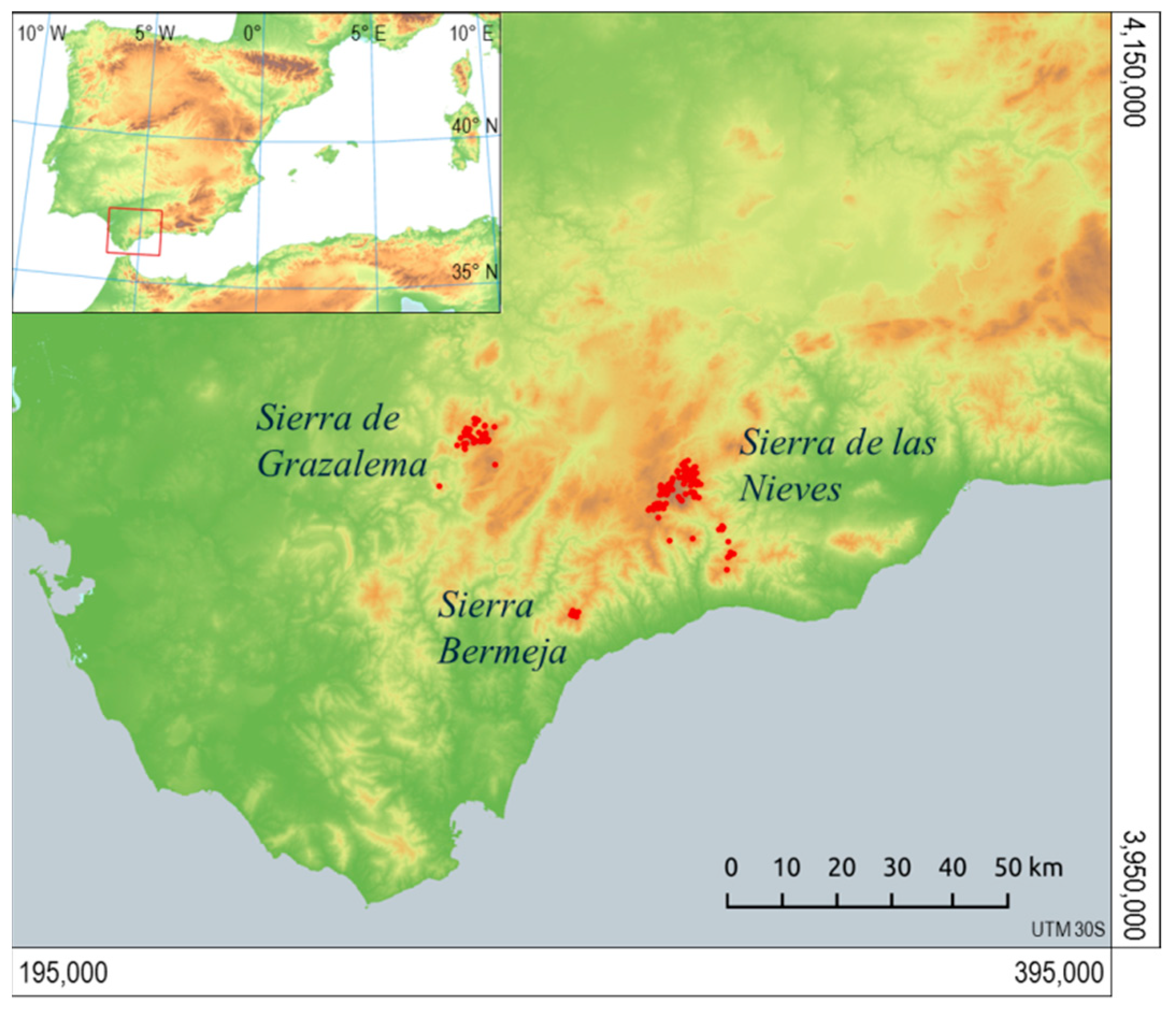
After reviewing the reference materials for the distribution of A. pinsapo [36], the operational scope of the Abies pinsapo Recovery Plan was considered adequate to frame the study [28]. The area of study encompasses the Ronda Mountains in their entirety, extending to the Gorda de Loja mountain range in the east and the Cordoban Subbaetic mountain range in the northeast; between the following geographical coordinates: 35°40′ N–37°30′ N and 4°10′ W–6°25′ W. For the purposes of the analysis and projection of results, the area of study was determined using UTM coordinates (zone 30, datum ETRS89) with the limits X: 195,000–395,000 and Y: 3,950,000–4,150,000 (Figure 1).
2.3. Observations of Presence
The presence of A. pinsapo was verified in sampling campaigns that took place in 2012 and 2013. A total of 141 stands of natural origin were sampled, in wich the presence of the different life stages was recorded. Three datasets were arranged for the SDM analysis, based on the presence of the life stages of interest. Two of those groups consisted of stands including individuals at either extreme of the age distribution (i.e., “sapling” and “mature”), while the third included all of the stands recorded (i.e., “whole”); these were defined as follows:
- Sapling: stands that included the presence of young individuals whose height did not exceed 40 cm; n = 41.
- Mature: stands that included the presence of individuals whose diameter at 130 cm above the ground (dbh) exceeded 20 cm; n = 134.
- Whole: included all of the stands of natural origin, regardless of the life stages they included; n = 141.
2.4. Predictor Variables
To serve as predictors, we selected three climate variables that defined the habitat of A. pinsapo, according to previous studies [31,37,38]: the growing degree days (GDD, °C·day), the values of which decrease with altitude and are a good predictor for species that inhabit the high mountains [39]; annual precipitation (AP, mm), which makes it possible to assess the species’ affinity for humid Bioclimates; and the warmest quarter precipitation (WQP, mm), which enabled us to characterise the Mediterranean nature of the species [40]. These variables were calculated using the monthly values available at a resolution of 100 m from the Andalusian Environmental Information Network (REDIAM, 2012) [41]:
where d is the number of days in the month m; Tm is the average temperature for the month m in degrees Celsius; Pm is the monthly precipitation for the month m in millimetres; Pmx is the precipitation for the month mx; and mx, mx+1, and mx+2 denote three consecutive months.
GDD = ∑ d · max [0 °C, Tm − 5 °C]
AP = ∑ Pm
WQP = Pmx + Pmx+1 + Pmx+2|max[(Tmx + Tmx+1 + Tmx+2), …]
With these data source and resolution, the correlation (Pearson) for each pair of variables was always less than 0.7 (Table A1).
The altitude was obtained from topographical variables derived from a digital elevation model (DEM) from the Food and Agriculture Organization of the United Nations (http://www.fao.org/soils-portal/, accessed on 9 February 2015).
2.5. Species Distribution Models
The potential distribution of A. pinsapo was modelled via MaxEnt and Bioclim using the dismo package for the R statistical computing environment [42,43,44,45]. MaxEnt, short for “maximum entropy”, is a machine-learning algorithm, while Bioclim is a so-called “envelope” algorithm. Both algorithms only require sets of presences, although MaxEnt needs a background dataset for calibration, which is used to characterise the environmental conditions of the area of study and is created using points selected at random from within the defined area [46]. All the models were calibrated parameters default setting.
Using Bioclim and MaxEnt, SDMs were generated in the area of the Ronda Mountains for the three groups chosen for the analysis (i.e., “sapling”, “mature”, and “whole”). To calibrate the models, we randomly selected 70 sampling points from among the 141 that were taken over the course of the sampling campaign. For the points selected, the presences in each age group were used to calibrate the respective habitat suitability models (the numbers of presences that were randomly obtained in each iteration are shown in Additional Table A2). From the remaining sampling points, we selected another 70 that were used to evaluate the models generated for the respective life stages. In this case, 10 iterations were performed for each algorithm and dataset (i.e., “sapling”, “mature”, and “whole”). The models were evaluated using the Area Under the ROC (Receiver Operating Characteristic) Curve (AUC), in which the AUC values of the 10 iterations for each model and dataset were averaged [47].
The habitat suitability models for the “sapling” and “mature” life stages were converted into potential distribution maps of a binary type (suitable/not suitable habitat) using a suitability threshold specifically defined for each algorithm (i.e., MaxEnt and Bioclim). The threshold selected was the value that maximised the sum of the true positive rate and true negative rate in each case.
2.6. Altitudinal Distribution Curves
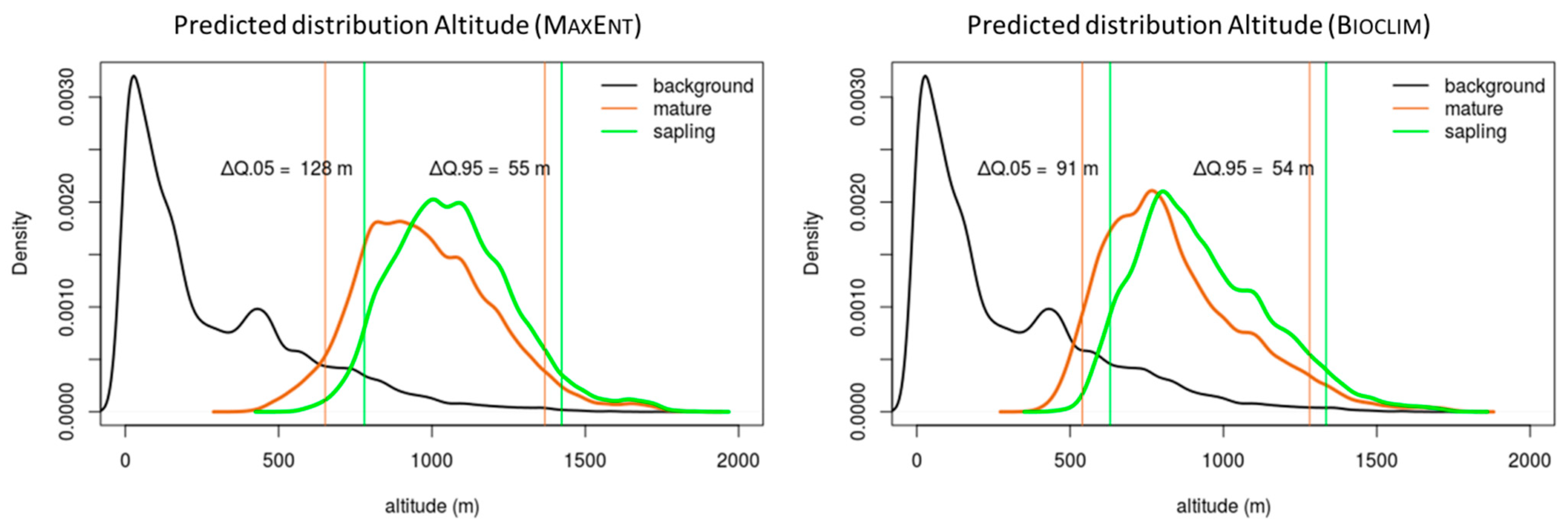
To analyse the potential altitudinal distribution of the two life stages (“sapling” and “mature”), we randomly selected 10,000 points within the area of suitability on each projected map and used their locations to obtain the altitude from the DEM. The 100,000 altitude values obtained for each age group (10 iterations × 10,000 points per projection) define the altitudinal distribution density in the area occupied by the age group in question. With regard to the altitudinal distribution, the 0.05 quantile indicates the lower limit of the altitudinal distribution (eliminating the outlier values) and the 0.95 quantile indicates the upper limit. The differences between the lower limits for the “mature” and “sapling” life stages indicate the altitudinal displacement at the lower limit, while the differences between the upper limits for the two groups indicate the altitudinal displacement at the upper limit. This analysis was performed for the models generated via MaxEnt as well as for those generated via Bioclim.
2.7. Persistence/Migration Map
To obtain suitability maps for each age group, the 10 iterations models for each group and algorithm were averaged, thereby creating a consensus map with continuous values. The averaged suitability map for the “whole” group was converted into a binary distribution map (suitable/not suitable habitat for the species) using the maximum of the sum of the sensitivity and specificity as the threshold for discrimination. Using the suitability maps for the “sapling” and “mature” life stages, we constructed a “persistence/migration” map for each algorithm, in which we identified the predominant trends (persistence and migration) with regard to population dynamics. The areas of persistence were defined as those where the suitability of the habitat was higher for individuals in the “mature” group than for those in the “sapling” group; conversely, in the areas of migration, the suitability was higher for the “sapling” group than for the “mature” group. In each instance, the distribution was delimited by the coverage of the binary map for the “whole” age group, which corresponds to the potential habitat of A. pinsapo.
3. Results
3.1. Species Distribution Models
The evaluation of the models produced AUC values (the average of the 10 iterations per algorithm and dataset) over 0.9, except for the sapling models built via Bioclim (Table 1). The MaxEnt models generally produced better results than the Bioclim models.
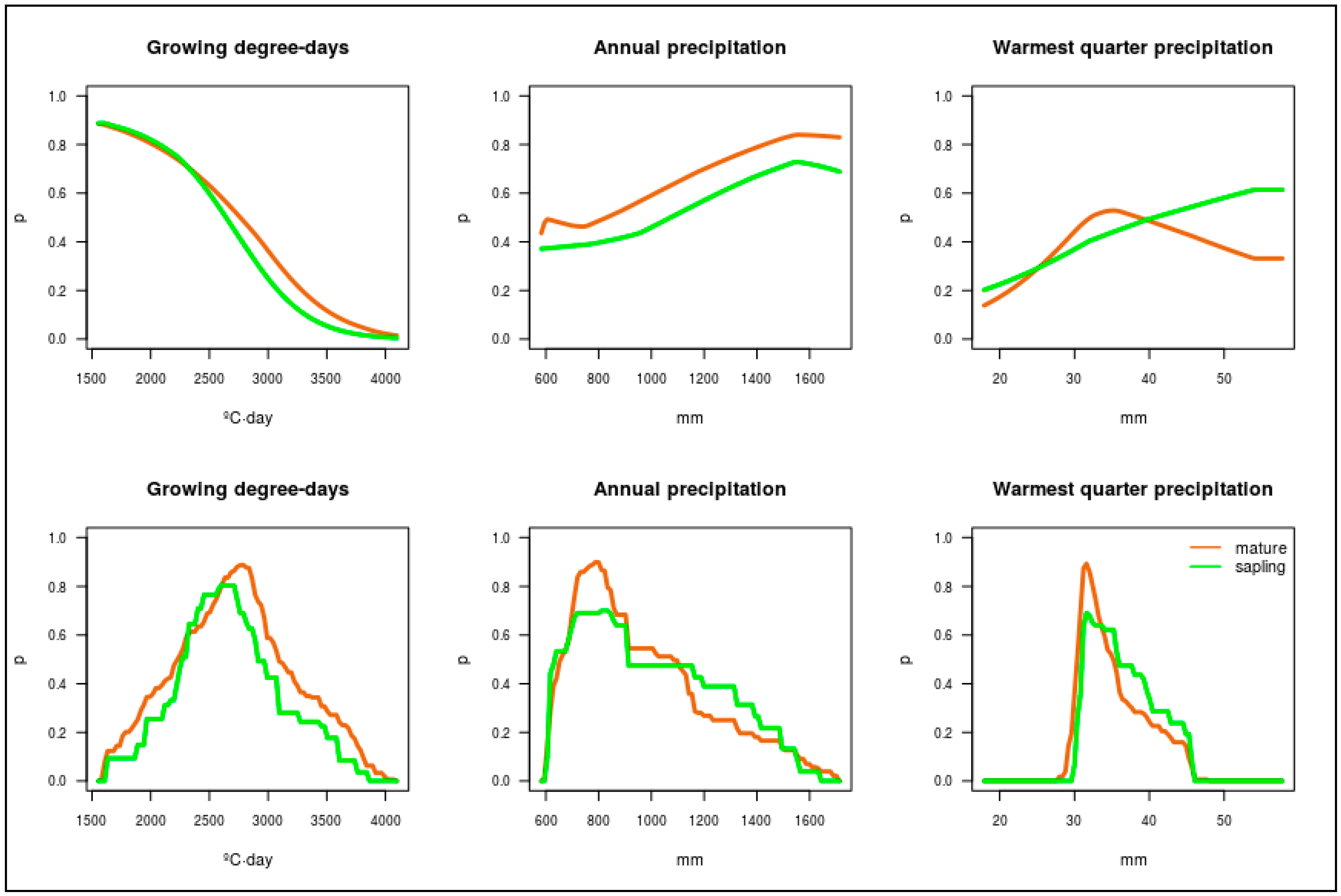
The variables’ response curves reveal a trend towards lower GDD values in the sapling group than in the mature group. In other words, compared to the mature specimens, saplings tend to be found in areas with lower temperatures. By contrast, the precipitation variables (annual and summer) reveal a trend towards higher values for saplings than for mature specimens (Figure 2). The variable that made the greatest percent contribution to the MaxEnt models was GDD, with values over 90%, followed by AP, with values of around 5%. Lastly, the values contributed by the WQP rarely exceeded 1%.
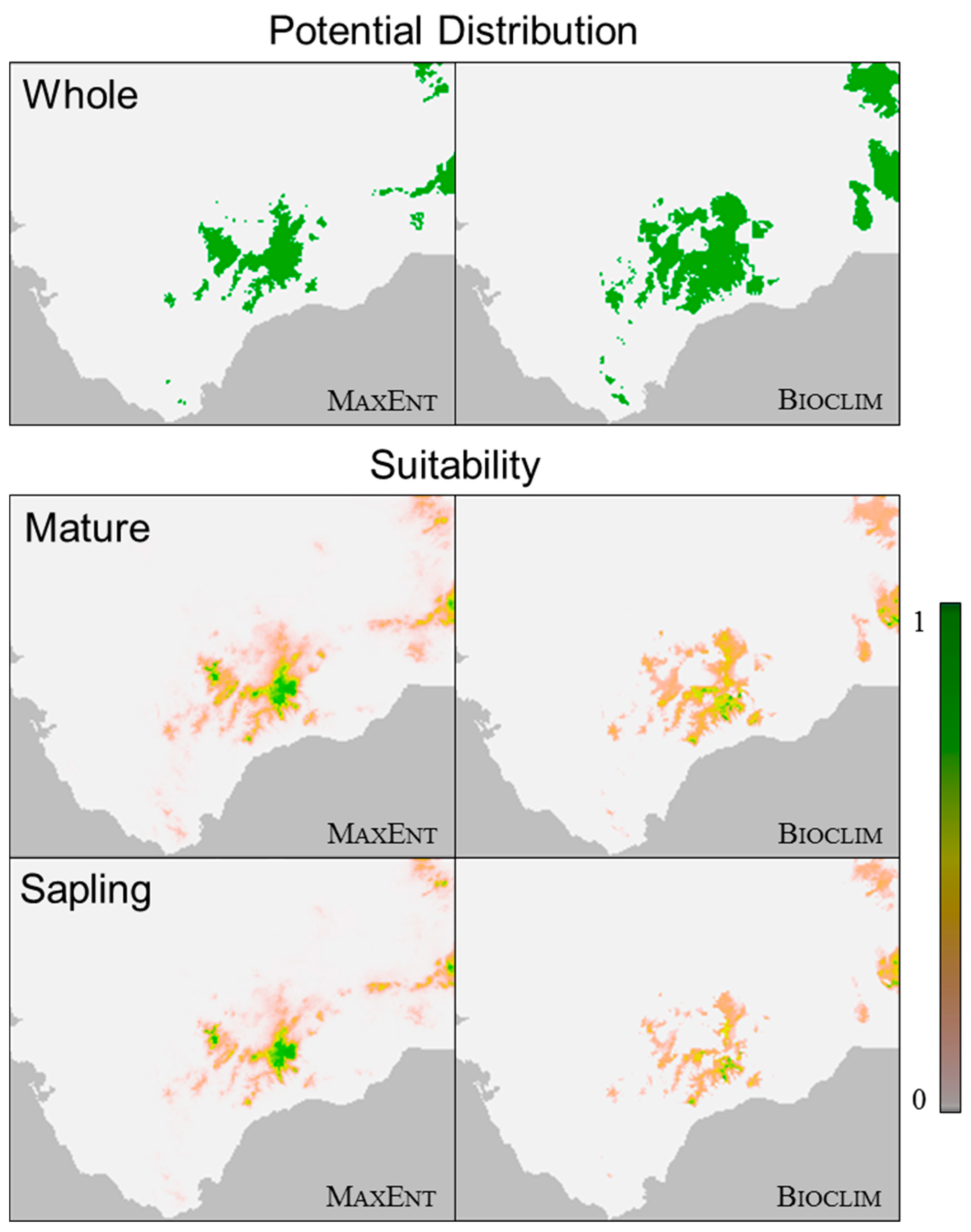
The predictions generated by Bioclim and MaxEnt regarding the optimal habitat of A. pinsapo were very similar. The models predicted its optimal distribution in the area that the species currently occupies within the Ronda Mountains and expanded the suitability of its distribution towards the east of the study area, in the direction of the Camarolos, Gorda de Loja, and Cordoban Subbaetic mountain ranges (Figure 3). The MaxEnt models concentrated the highest suitability values in the areas that the species currently occupies (i.e., the higher parts of the Sierra de las Nieves and Grazalema mountain ranges), while Bioclim distributed the suitability values across a somewhat larger area.
The habitat suitability predictions presented differences between the life stages. The suitability prediction for the “mature” group was very similar to that for the “whole” group, owing to the low number of sampling points where no mature individuals were recorded. The distribution for the “sapling” group was associated with the higher altitudes in the Ronda Mountains, with a slight contraction of the optimal area compared to that for the “mature” group (Figure 3).
3.2. Altitudinal Distribution Curves
The models for the “sapling” group provided evidence of displacement towards higher altitudes (Figure 4), in comparison to those for the “mature” group. Bioclim and MaxEnt both revealed this pattern, although the curves generated by Bioclim occupied lower altitudes than those generated by MaxEnt. The analyses also revealed that the lower limit for the projected distribution of A. pinsapo in the Ronda Mountains lay between 540 and 780 m, while the upper limit lay between 1281 and 1423 m. The lower distribution limit for the “sapling” group was 128 m above the lower limit for the “mature” group with MaxEnt, and 91 m with Bioclim. In terms of the upper distribution limit for A. pinsapo, the “sapling” group was 55 m above the “mature” group in the projections generated by MaxEnt, and 54 m in those generated by Bioclim (Table 2).
There were greater differences between the lower limits for the life stages than there were between the upper limits: 73 m in the case of MaxEnt and 37 m in the case of Bioclim.
3.3. Persistence/Migration Map
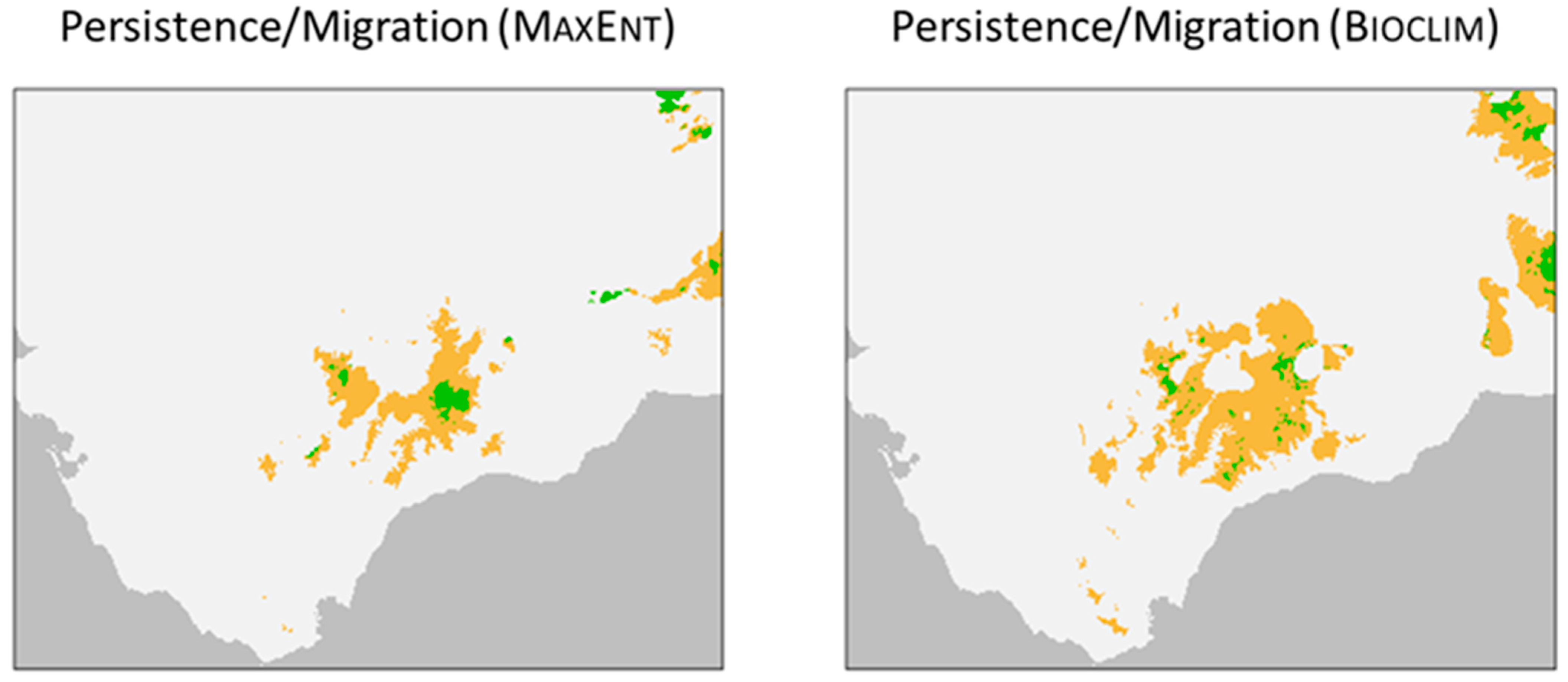
The binary distribution of the “mature” age group is very similar to that of the “whole” group. Moreover, the suitability values for the “mature” age group are higher than those for the “sapling” age group in the majority of the optimal habitats for A. pinsapo (Figure 5). This is the area that represents the species’ tendency towards persistence under changing climatic conditions (at least as defined by the predictor variables selected). The suitability values for the “sapling” age group are higher than those for the “mature” age group only in the highest parts of the optimal habitat for A. pinsapo. These parts of the habitat represent the areas in which the tendency towards migration predominates in the population dynamics under changing environmental conditions. The areas of migration are unconnected, with variations in the projections generated via MaxEnt and Bioclim, and are located in the Grazalema, Sierra de las Nieves, Bermeja, Torcal de Antequera, Gorda de Loja, and Cordoban Subbaetic mountain ranges (Figure 5).
4. Discussion
The SDMs reveal differences in the habitat distributions for different life stages of A. pinsapo. The distribution of the “mature” age group is indistinguishable from that of the species as a whole; therefore, the species’ realised niche can be considered equivalent to that of this age group. The projected species’ optimal habitat comprises the areas it currently occupies and extends to the baseline areas of the Ronda Mountains, eventually attaining geographical continuity among the locations studied, which are currently fragmented. Likewise, the species’ potential habitat is projected to include the Gorda de Loja and Cordoban Subbaetic mountain ranges in the east of the area of study. The predicted distribution of the “sapling” group, which corresponds to the species’ reproductive niche [21], reveals a contraction of the optimal area in comparison to the realised niche. The models geographically isolate the locations, meaning that the saplings’ potential distribution is restricted to the higher altitudes.
Today, the baseline areas no longer possess optimal conditions for the establishment of the species. This has resulted in populations that are suffering from structural disequilibrium, where mature individuals are prevailing and there is a lack of recruitment. Differences in growth and mortality in the populations of A. pinsapo throughout the altitudinal gradient have been attributed to variations in the water balance and the strong competition for water resources in the lower areas [48,49,50,51,52]. The bands of vegetation located in the lower areas constitute the trailing edge in the migratory dynamic and occupy the bottom 90–130 m of the altitudinal gradient, depending on the model. In the higher areas, where the temperatures are lower and the annual water balance is higher, colonisation may occur as a result of conditions that are increasingly conducive to the establishment of A. pinsapo. This leading altitudinal edge comprises the top 55 m of the population. However, colonisation above the upper limit for the species may be hindered by a multitude of factors (e.g., damage by frost and winter desiccation, heat flux or radiative warming of rooting zone) [53]. Even though the altitudinal displacement of populations of A. pinsapo has been proposed before as a consequence of a better energy balance at high altitudes [48], the speed of the altitudinal displacement of these populations has not yet been described in the manner that it has been carried out in other specific studies on species distribution displacement [5,7,11,15,16,17,54].
In the majority of their current geographical distribution, the populations of A. pinsapo consist of forests that are dominated by mature individuals, where the stability of the system may hinder the recruitment. In the models, the suitability of the “mature” group is higher than that of the “sapling” group throughout most of the species’ distribution, thereby demonstrating a tendency towards persistence, rather than migration. In areas of higher altitude, the forests are less dense, and in the more exposed areas, the individual specimens are smaller [50,55]. Such conditions are conducive to the establishment of younger individuals, and the models reveal them to be more suitable for the “sapling” group than the “mature” group. Geographically, these areas are associated with the processes of migration. Even though the areas identified as “migration” differ in size depending on the model used (Figure 5), their presence indicates the location of forests that have a better structure of different life stages.
Even though an increasing number of studies have linked the altitudinal displacement of the plants’ distribution with climate change, the detected changes—in both the leading and trailing edges—may be the result of other factors (sampling and data limitations, use soil or successive changes, silvicultural practices, presence of wild herbivores) [2,12,54]. Actually, even though the design of the sampling process was significantly conditioned by the prior knowledge of the presence of mature individuals (which could therefore have led to population bias at the sampling points), the results demonstrate an unequal distribution on the altitudinal gradient for saplings, suggesting a tendency for this group to occupy higher elevations. Moreover, although higher survival rates have been described for seedlings that grow in clearings [56,57], the presence of young specimens located far away from consolidated A. pinsapo forest was invariably observed in the samples as the result of planting. That suggests that it may be due to the Allee effect, in which establishment (i.e., the sapling group) is conditioned by the degree of persistence (i.e., the mature group) [58].
The powerful effect of persistence in the baseline areas of the distribution of A. pinsapo may be reinforced by the presence of numerous individuals and small, isolated copses that are left over from previous wildfires from which the forest was unable to recover. In fact, from 1968 to 2013, more than 110 ha of A. pinsapo forest have been lost due to wildfires, most of them in their lower areas on peridotites [59]. These areas at low altitude in which there is hardly any regeneration were included in the sampling. The effect on A. pinsapo of the recent wildfire in Sierra Bermeja (September 2021) has not yet been evaluated. Additionally, the actions that have been taken to preserve the species since the middle of the last century have significantly shaped the formation of coeval forests in the baseline areas, where the density—and the competition between individuals—has led to decay and high mortality and impeded recruitment [49,50]. Moreover, drough and competition affect the susceptibility of A. pinsapo to infestation by pests, and especially by the basidiomycete Heterobasidion annosum (Fr.) Bref. [60].
Finally, the optimal habitat of A. pinsapo in the Ronda Mountains lies between altitudes of 650 m and 1350 m. The most unfavourable conditions for the species indicate a trailing edge in the lower 110 m of its distribution. There, the species is persisting under unsuitable conditions, giving rise to what has been called “time-delayed extinction in a situation of disequilibrium” [24]. In the upper 55 m of its distribution, we find the leading edge of an altitudinal migration that is limited by the height of the Ronda Mountains themselves The differences in the altitudinal shifts between the trailing and leading edges demonstrate a population dynamic in which the leading edge is smaller than the trailing edge, resulting in a so-called “lean pattern” [26].
5. Conclusions
The realised niche of A. pinsapo is different to its reproductive niche, which indicates that the current environmental conditions do not allow the species to complete its lifecycle in all of the areas in which it is currently present. These differences may indicate an altitudinal displacement in its distribution owing to the changing climatic conditions in the Ronda Mountains.
Even though this pattern will not cause the populations to become extinct in the short term, it may threaten their viability if the conditions that are producing the contraction at the lower limit persist over time.
Author Contributions
Conceptualisation, A.G.-H., D.N.-L. and J.P.; methodology and formal analysis, A.G.-H. and D.N.-L.; writing—original draft preparation, A.G.-H.; writing—review and editing, D.N.-L., J.P. and F.A.-S.; project administration and funding acquisition, F.A.-S. All authors have read and agreed to the published version of the manuscript.
Funding
This research was funded by (i) Spanish government, State R&D Program Oriented to the Challenges of the Society: MED-REFUGIA Research Project (RTI2018-101714-B-I00); (ii) Andalusian Plan for Research, Development and Innovation: OROMEDREFUGIA Research Project (P18-RT-4963); (iii) ERDF Operational Programme in Andalusia (EU regional programme): RELIC-FLORA 2 Research Project (B-RNM-404-UGR18); and (iv) State Program for the Promotion of Scientific Research and Excellence Technique: PALEOPINSAPO Research Project (CSO2017-83576-P). The APC was funded by (i) Spanish government, State R&D Program Oriented to the Challenges of the Society: MED-REFUGIA Research Project (RTI2018-101714-B-I00); and (ii) Andalusian Plan for Research, Development and Innovation: OROMEDREFUGIA Research Project (P18-RT-4963).
Institutional Review Board Statement
Not applicable.
Informed Consent Statement
Not applicable.
Data Availability Statement
The data used in this study are available at https://zenodo.org/doi/10.5281/zenodo.10810414.
Acknowledgments
We thank José López-Quintanilla (Department of the Environment, Andalusian Government) for facilitating our fieldwork in the Baetics Mountains.
Conflicts of Interest
The authors declare no conflict of interest. The funders had no role in the design of the study; in the collection, analyses, or interpretation of data; in the writing of the manuscript, or in the decision to publish the results.
Correction Statement
This article has been republished with a minor correction to the Data Availability Statement. This change does not affect the scientific content of the article.
Appendix A

Table A1.
Correlations between environmental variables (Pearson). GDD: growing degree days; AP: annual precipitation; WQP: warmest quarter precipitation.
Table A1.
Correlations between environmental variables (Pearson). GDD: growing degree days; AP: annual precipitation; WQP: warmest quarter precipitation.
| GDD | AP | WQP | |
|---|---|---|---|
| GDD | 1 | ||
| AP | −0.209 | 1 | |
| WQP | −0.296 | 0.531 | 1 |
Table A2.
Number of presences in the life stages (mature and sapling) selected in each of the 10 iterations of the SDMs. Of the 141 sampling points recorded in the Baetic System, 70 samples were randomly selected to calibrate the model in each iteration, while a further 70 were chosen for the evaluation.
| Training | Evaluation | |||
|---|---|---|---|---|
| Subset | Mature | Sapling | Mature | Sapling |
| 1 | 66 | 19 | 67 | 22 |
| 2 | 68 | 21 | 65 | 20 |
| 3 | 68 | 23 | 65 | 18 |
| 4 | 67 | 23 | 66 | 18 |
| 5 | 65 | 21 | 68 | 19 |
| 6 | 67 | 23 | 66 | 18 |
| 7 | 67 | 23 | 66 | 18 |
| 8 | 65 | 22 | 68 | 19 |
| 9 | 64 | 17 | 69 | 24 |
| 10 | 68 | 19 | 65 | 22 |
References
- Ackerly, D.D.; Schwilk, D.W.; Webb, C.O. Niche evolution and adaptive radiation: Testing the order of trait divergence. Ecology 2006, 87, S50–S61. [Google Scholar] [CrossRef]
- Benito, B.; Lorite, J.; Pérez-Pérez, R.; Gómez-Aparicio, L.; Peñas, J. Forecasting plant range collapse in a Mediterranean hotspot: When dispersal uncertainties matter. Divers. Distrib. 2014, 20, 72–83. [Google Scholar] [CrossRef]
- Kingsolver, J.G.; Pfennig, D.W.; Servedio, M.R. Migration, local adaptation and the evolution of plasticity. Trends Ecol. Evol. 2002, 17, 540–541. [Google Scholar] [CrossRef]
- Valladares, F.; Matesanz, S.; Guilhaumon, F.; Araújo, M.B.; Balaguer, L.; Benito-Garzón, M.; Cornwell, W.; Gianoli, E.; van Kleunen, M.; Naya, D.E.; et al. The effects of phenotypic plasticity and local adaptation on forecasts of species range shifts under climate change. Ecol. Lett. 2014, 17, 1351–1364. [Google Scholar] [CrossRef]
- Benito, B.; Lorite, J.; Peñas, J. Simulating potential effects of climatic warming on altitudinal patterns of key species in Mediterranean-Alpine ecosystems. Clim. Change 2011, 108, 471–483. [Google Scholar] [CrossRef]
- Burrows, M.T.; Schoeman, D.S.; Richardson, A.J.; Molinos, J.G.; Hoffmann, A.; Buckley, L.B.; Moore, P.J.; Brown, C.J.; Bruno, J.F.; Duarte, C.M.; et al. Geographical limits to species-range shifts are suggested by climate velocity. Nature 2014, 507, 492–495. [Google Scholar] [CrossRef] [PubMed]
- Chen, I.-C.; Hill, J.K.; Ohlemüller, R.; Roy, D.B.; Thomas, C.D. Rapid range shifts of species associated with high levels of climate warming. Science 2011, 333, 1024–1026. [Google Scholar] [CrossRef] [PubMed]
- Parmesan, C. Ecological and evolutionary responses to recent climate change. Annu. Rev. Ecol. Evol. Syst. 2006, 37, 637–669. [Google Scholar] [CrossRef]
- Parmesan, C.; Yohe, G. A globally coherent fingerprint of climate change impacts across natural systems. Nature 2003, 421, 37–42. [Google Scholar] [CrossRef]
- Bell, D.M.; Bradford, J.B.; Lauenroth, W.K. Early indicators of change: Divergent climate envelopes between tree life stages imply range shifts in the Western United States. Glob. Ecol. Biogeogr. 2014, 23, 168–180. [Google Scholar] [CrossRef]
- Jump, A.S.; Mátyás, C.; Peñuelas, J. The altitude-for-latitude disparity in the range retractions of woody species. Trends Ecol. Evol. 2009, 24, 694–701. [Google Scholar] [CrossRef] [PubMed]
- Zhu, K.; Woodall, C.W.; Clark, J.S. Failure to migrate: Lack of tree range expansion in response to climate change. Glob. Change Biol. 2012, 18, 1042–1052. [Google Scholar] [CrossRef]
- Lenoir, J.; Gégout, J.-C.; Pierrat, J.-C.; Bontemps, J.-D.; Dhôte, J.-F. Differences between tree species seedling and adult altitudinal distribution in mountain forests during the Recent Warm Period (1986–2006). Ecography 2009, 32, 765–777. [Google Scholar] [CrossRef]
- Matías, L.; Jump, A.S. Asymmetric changes of growth and reproductive investment herald altitudinal and latitudinal range shifts of two woody species. Glob. Change Biol. 2015, 21, 882–896. [Google Scholar] [CrossRef] [PubMed]
- Peñuelas, J.; Ogaya, R.; Boada, M.; Jump, A. Migration, invasion and decline: Changes in recruitment and forest structure in a warming-linked shift of European beech forest in Catalonia (NE Spain). Ecography 2007, 30, 829–837. [Google Scholar] [CrossRef]
- Peñuelas, J.; Boada, M. A global change-induced biome shift in the Montseny Mountains (NE Spain). Glob. Change Biol. 2003, 9, 131–140. [Google Scholar] [CrossRef]
- Urli, M.; Delzon, S.; Eyermann, A.; Couallier, V.; García-Valdés, R.; Zavala, M.A.; Porté, A.J. Inferring shifts in tree species distribution using asymmetric distribution curves: A case study in the Iberian Mountains. J. Veg. Sci. 2014, 25, 147–159. [Google Scholar] [CrossRef]
- Araújo, M.B.; Pearson, R.G. Equilibrium of species’ distributions with climate. Ecography 2005, 28, 693–695. [Google Scholar] [CrossRef]
- Svenning, J.-C.; Sandel, B. Disequilibrium vegetation dynamics under future climate change. Am. J. Bot. 2013, 100, 1266–1286. [Google Scholar] [CrossRef]
- Corlett, R.T.; Westcott, D.A. Will plant movements keep up with climate change? Trends Ecol. Evol. 2013, 28, 482–488. [Google Scholar] [CrossRef]
- Bykova, O.; Chuine, I.; Morin, X.; Higgins, S.I. Temperature dependence of the reproduction niche and its relevance for plant species distributions. J. Biogeogr. 2012, 39, 2191–2200. [Google Scholar] [CrossRef]
- Elith, J.; Kearney, M.; Phillips, S.J. The art of modelling range-shifting species. Methods Ecol. Evol. 2010, 1, 330–342. [Google Scholar] [CrossRef]
- Thuiller, W.; Albert, C.; Araújo, M.B.; Berry, P.M.; Cabeza, M.; Guisan, A.; Hickler, T.; Midgley, G.F.; Paterson, J.; Schurr, F.M.; et al. Predicting global change impacts on plant species’ distributions: Future challenges. Perspect. Plant Ecol. Evol. Syst. 2008, 9, 137–152. [Google Scholar] [CrossRef]
- Schurr, F.M.; Pagel, J.; Cabral, J.S.; Groeneveld, J.; Bykova, O.; O’Hara, R.B.; Hartig, F.; Kissling, W.D.; Linder, H.P.; Midgley, G.F.; et al. How to understand species’ niches and range dynamics: A demographic research agenda for biogeography. J. Biogeogr. 2012, 39, 2146–2162. [Google Scholar] [CrossRef]
- Lenoir, J.; Svenning, J.-C. Latitudinal and elevational range shifts under contemporary climate change. In Encyclopedia of Biodiversity; Levin, S.A., Ed.; Academic Press: Waltham, MA, USA, 2013; pp. 599–611. ISBN 978-0-12-384720-1. [Google Scholar]
- Lenoir, J.; Svenning, J.-C. Climate-related range shifts—A global multidimensional synthesis and new research directions. Ecography 2015, 38, 15–28. [Google Scholar] [CrossRef]
- Arista, M.; Knees, S.; Gardner, M. Abies Pinsapo Var. Pinsapo. IUCN Red List of Threatened Species 2011; IUCN Global Species Programme Red List Unit: Cambridge, UK, 2011. [Google Scholar] [CrossRef]
- Junta de Andalucía/Consejería de Medio Ambiente. Plan de Recuperación del Pinsapo. Available online: http://www.juntadeandalucia.es/boja/2011/25/boletin.25.pdf (accessed on 23 January 2013).
- Intergovernmental Panel on Climate Change (IPCC). Climate Change 2014: Synthesis Report; Contribution of Working Groups I, II and III to the Fifth Assessment Report of the Intergovernmental Panel on Climate Change; Core Writing Team, Pachauri, R.K., Meyer, L., Eds.; Intergovernmental Panel on Climate Change (IPCC): Geneva, Switzerland, 2014. [Google Scholar]
- Farjon, A. Pinaceae: Drawing and Descriptions of the Genera Abies, Cedrus, Pseudolarix, Keteleeria, Nothotsuga, Tsuga, Cathaya, Pseudotsuga, Larix and Picea; Koeltz Scientific Books: Königstein, Germany, 1990; ISBN 978-1-878762-04-7. [Google Scholar]
- Linares, J.C.; Carreira, J.A. El pinsapo, abeto endémico andaluz. O, ¿Qué hace un tipo como tú en un sitio como éste? Ecosistemas 2006, 15, 171–191. [Google Scholar]
- Govaerts, R.; Farjon, A. Pinaceae. Available online: http://wcsp.science.kew.org (accessed on 2 February 2021).
- Balao, F.; Lorenzo, M.T.; Sánchez-Robles, J.M.; Paun, O.; García-Castaño, J.L.; Terrab, A. Early diversification and permeable species boundaries in the Mediterranean firs. Ann. Bot. 2020, 125, 495–507. [Google Scholar] [CrossRef]
- Sękiewicz, K.; Sękiewicz, M.; Jasińska, A.K.; Boratyńska, K.; Iszkuło, G.; Romo, A.; Boratyński, A. Morphological diversity and structure of West Mediterranean Abies species. Plant Biosyst. 2013, 147, 125–134. [Google Scholar] [CrossRef]
- Terrab, A.; Talavera, S.; Arista, M.; Paun, O.; Stuessy, T.F.; Tremetsberger, K. Genetic diversity at chloroplast microsatellites (CpSSRs) and geographic structure in endangered West Mediterranean firs (Abies spp., Pinaceae). Taxon 2007, 56, 409–416. [Google Scholar] [CrossRef]
- Guzmán Álvarez, J.R.; Catalina, M.A.; Navarro Cerrillo, R.M.; López Quintanilla, J.; Sánchez-Salguero, R. Los paisajes del pinsapo a través del tiempo. In Los Pinsapares en Andalucia (Abies pinsapo Boiss.): Conservación y Sostenibilidad en el Siglo XXI; López Quintanilla, J., Ed.; Junta de Andalucía-Universidad de Córdoba: Cordoba, Spain, 2013; pp. 111–149. ISBN 978-84-9927-137-8. [Google Scholar]
- Arista, M.; Herrera, F.J.; Talavera, S. Biología del Pinsapo; Consejería de Medio Ambiente, Junta de Andalucía: Sevilla, Spain, 1997. [Google Scholar]
- Valladares, A. Abetales de Abies pinsapo Boiss. In Bases Ecológicas Preliminares para la Conservación de los Tipos de Hábitat de Interés Comunitario en España; Ministerio Medio Ambiente y Medio Rural y Marino: Madrid, Spain, 2009; Volume 9520, ISBN 978-84-491-0911-9. [Google Scholar]
- Skov, F.; Svenning, J.-C. Potential impact of climatic change on the distribution of forest herbs in Europe. Ecography 2004, 27, 366–380. [Google Scholar] [CrossRef]
- Aussenac, G. Ecology and ecophysiology of circum-Mediterranean firs in the context of climate change. Ann. For. Sci. 2002, 59, 823–832. [Google Scholar] [CrossRef]
- REDIAM Red de Información Ambiental de Andalucía. Available online: http://www.juntadeandalucia.es/medioambiente/site/rediam (accessed on 17 January 2012).
- Phillips, S.J.; Anderson, R.P.; Schapire, R.E. Maximum entropy modeling of species geographic distributions. Ecol. Model. 2006, 190, 231–259. [Google Scholar] [CrossRef]
- Nix, H.A. A biogeographic analysis of Australian elapid snakes. In Atlas of Elapid Snakes of Australia: Australian Flora and Fauna; Longmore, R., Ed.; Bureau of Flora and Fauna: Camberra, Australia, 1986; pp. 4–15. [Google Scholar]
- Hijmans, R.J.; Phillips, S.J.; Leathwick, J.; Elith, J. Package ‘Dismo’. Species Distribution Modeling. R Package, Version 0.7-17; Institute for Statistics and Mathematics: Vienna, Austria, 2014. [Google Scholar]
- R Core Team. R: A Language and Environment for Statistical Computing; R Foundation for Statistical Computing: Vienna, Austria, 2012; Available online: http://www.r-project.org/ (accessed on 21 January 2013).
- Elith, J.; Phillips, S.J.; Hastie, T.; Dudík, M.; Chee, Y.E.; Yates, C.J. A statistical explanation of MaxEnt for ecologists. Divers. Distrib. 2011, 17, 43–57. [Google Scholar] [CrossRef]
- Jiménez-Valverde, A. Insights into the area under the receiver operating characteristic curve (AUC) as a discrimination measure in species distribution modelling. Glob. Ecol. Biogeogr. 2012, 21, 498–507. [Google Scholar] [CrossRef]
- Lechuga, V.; Carraro, V.; Viñegla, B.; Carreira, J.A.; Linares, J.C. Carbon limitation and drought sensitivity at contrasting elevation and competition of Abies pinsapo forests. Does experimental thinning enhance water supply and carbohydrates? Forests 2019, 10, 1132. [Google Scholar] [CrossRef]
- Linares, J.C.; Camarero, J.J.; Carreira, J.A. Interacting effects of changes in climate and forest cover on mortality and growth of the southernmost European fir forests. Glob. Ecol. Biogeogr. 2009, 18, 485–497. [Google Scholar] [CrossRef]
- Linares, J.C.; Delgado-Huertas, A.; Camarero, J.J.; Merino, J.; Carreira, J.A. Competition and drought limit the response of water-use efficiency to rising atmospheric carbon dioxide in the Mediterranean fir Abies pinsapo. Oecologia 2009, 161, 611–624. [Google Scholar] [CrossRef]
- Linares, J.C.; Covelo, F.; Carreira, J.A.; Merino, J.Á. Phenological and water-use patterns underlying maximum growing season length at the highest elevations: Implications under climate change. Tree Physiol. 2012, 32, 161–170. [Google Scholar] [CrossRef]
- Sánchez-Salguero, R.; Ortíz, C.; Covelo, F.; Ochoa, V.; García-Ruíz, R.; Seco, J.I.; Carreira, J.A.; Merino, J.Á.; Linares, J.C. Regulation of water use in the southernmost European fir (Abies pinsapo Boiss.): Drought avoidance matters. Forests 2015, 6, 2241–2260. [Google Scholar] [CrossRef]
- Körner, C. A re-assessment of high elevation treeline positions and their explanation. Oecologia 1998, 115, 445–459. [Google Scholar] [CrossRef]
- Lenoir, J.; Gégout, J.C.; Marquet, P.A.; de Ruffray, P.; Brisse, H. A significant upward shift in plant species optimum elevation during the 20th century. Science 2008, 320, 1768–1771. [Google Scholar] [CrossRef]
- Linares, J.C.; Viñegla, B.; Carreira, J.A. Caracterización estructural de poblaciones de Abies pinsapo Boiss. en la sierra de Yunquera (Málaga). Iniciación Investig. 2010, 2, a7. [Google Scholar]
- Arista, M. Germinación de las semillas y supervivencia de las plántulas de Abies pinsapo Boiss. Acta Bot. Malacit. 1993, 18, 173–177. [Google Scholar] [CrossRef]
- Arista, M. Supervivencia de las plántulas de Abies pinsapo Boiss. en su hábitat natural. An. Jardín Bot. Madr. 1994, 51, 193–198. [Google Scholar]
- Holt, R.D. Bringing the hutchinsonian niche into the 21st century: Ecological and evolutionary perspectives. Proc. Natl. Acad. Sci. USA 2009, 106, 19659–19665. [Google Scholar] [CrossRef] [PubMed]
- Catalina, M.A. Incendios en el pinsapar. In Los Pinsapares en Andalucia (Abies pinsapo Boiss.): Conservación y Sostenibilidad en el Siglo XXI; López Quintanilla, J., Ed.; Junta de Andalucía-Universidad de Córdoba: Córdoba, Spain, 2013; pp. 371–373. ISBN 978-84-9927-137-8. [Google Scholar]
- García Esteban, L.; de Palacios, P.; Rodríguez-Losada Aguado, L. Abies Pinsapo forests in Spain and Morocco: Threats and conservation. Oryx 2010, 44, 276–284. [Google Scholar] [CrossRef]
Figure 1.
Study area in the Ronda Mountains (Baetic System). Stands sampled are represented by points which were used as verified presence of Abies pinsapo to calibrate the distribution models for the species.
Figure 1.
Study area in the Ronda Mountains (Baetic System). Stands sampled are represented by points which were used as verified presence of Abies pinsapo to calibrate the distribution models for the species.

Figure 2.
Response curves for the “mature” (brown) and “sapling” (light green) models for the three predictor variables: Growing degree-days, Annual precipitation, and Warmest quarter precipitation (MaxEnt, top; Bioclim, bottom).
Figure 2.
Response curves for the “mature” (brown) and “sapling” (light green) models for the three predictor variables: Growing degree-days, Annual precipitation, and Warmest quarter precipitation (MaxEnt, top; Bioclim, bottom).

Figure 3.
Models in MaxEnt (left) and Bioclim (right) for Abies pinsapo Boiss. in the Baetic System. The figures show the potential habitat (in binary terms) for the species (“whole”, i.e., all ages, on the top) and suitability (0 to 1) for the “mature” group (centre) and “sapling” group (bottom).
Figure 3.
Models in MaxEnt (left) and Bioclim (right) for Abies pinsapo Boiss. in the Baetic System. The figures show the potential habitat (in binary terms) for the species (“whole”, i.e., all ages, on the top) and suitability (0 to 1) for the “mature” group (centre) and “sapling” group (bottom).

Figure 4.
Altitudinal distributions of the “sapling” and “mature” life stages. The density curves show the distributions of both groups throughout the altitudinal gradient, which were obtained using the potential habitats projected by the models (MaxEnt and Bioclim). The 0.95 and 0.05 quantiles were identified as the upper and lower limits, respectively. The altitudinal displacement of the upper and lower limits was calculated based on the difference between the quantiles (ΔQ) of the two life stages.

Figure 5.
Persistence versus migration. Distributions projected using MaxEnt and Bioclim in the Baetic System. Persistence (brown) is shown in those areas where the suitability of the habitat is greater for the “mature” group than it is for the “sapling” group, while the migration areas (light green) are those where the suitability of the habitat is greater for the “sapling” group than it is for the “mature” group.

Table 1.
Average evaluation (10 iterations) of the distribution models for the different life stages: whole, mature, and sapling.
Table 1.
Average evaluation (10 iterations) of the distribution models for the different life stages: whole, mature, and sapling.
| AUC | |||
|---|---|---|---|
| Whole | Mature | Sapling | |
| MaxEnt | 0.9819 | 0.9815 | 0.9880 |
| Bioclim | 0.9201 | 0.9234 | 0.8483 |
AUC: area under the curve.
Table 2.
Altitudinal limits of the projections (MaxEnt and Bioclim) for Abies pinsapo Boiss. in the Baetic System.
Table 2.
Altitudinal limits of the projections (MaxEnt and Bioclim) for Abies pinsapo Boiss. in the Baetic System.
| MaxEnt | Bioclim | |||||
|---|---|---|---|---|---|---|
| Mature | Sapling | ΔQ | Mature | Sapling | ΔQ | |
| Q.05 | 652 | 780 | 128 | 540 | 631 | 91 |
| Q.95 | 1368 | 1423 | 55 | 1281 | 1335 | 54 |
Elevation (masl). Q.05: 0.05 quantile in the altitudinal distribution; Q.95: 0.95 quantile in the altitudinal distribution. ΔQ: difference between life stages limits (0.05, lower limit; 0.95, upper limit).
Publisher’s Note: MDPI stays neutral with regard to jurisdictional claims in published maps and institutional affiliations. |
© 2021 by the authors. Licensee MDPI, Basel, Switzerland. This article is an open access article distributed under the terms and conditions of the Creative Commons Attribution (CC BY) license (https://creativecommons.org/licenses/by/4.0/).
Share and Cite
MDPI and ACS Style
González-Hernández, A.; Nieto-Lugilde, D.; Peñas, J.; Alba-Sánchez, F. Lean Pattern in an Altitude Range Shift of a Tree Species: Abies pinsapo Boiss. Forests 2021, 12, 1451. https://0-doi-org.brum.beds.ac.uk/10.3390/f12111451
AMA Style
González-Hernández A, Nieto-Lugilde D, Peñas J, Alba-Sánchez F. Lean Pattern in an Altitude Range Shift of a Tree Species: Abies pinsapo Boiss. Forests. 2021; 12(11):1451. https://0-doi-org.brum.beds.ac.uk/10.3390/f12111451
Chicago/Turabian StyleGonzález-Hernández, Antonio, Diego Nieto-Lugilde, Julio Peñas, and Francisca Alba-Sánchez. 2021. "Lean Pattern in an Altitude Range Shift of a Tree Species: Abies pinsapo Boiss." Forests 12, no. 11: 1451. https://0-doi-org.brum.beds.ac.uk/10.3390/f12111451
Note that from the first issue of 2016, this journal uses article numbers instead of page numbers. See further details here.