Integration of Forest Growth Component in the FEST-WB Distributed Hydrological Model: The Bonis Catchment Case Study

Abstract

In this paper, the FEST-FOREST model is presented. A FOREST module is written in the FORTRAN-90 programming language, and was included in the FEST-WB distributed hydrological model delivering the FEST-FOREST model. FEST-FOREST is a process-based dynamic model allowing the simulation at daily basis of gross primary production (GPP) and net primary production (NPP) together with the carbon allocation of a homogeneous population of trees (same age, same species). The model was implemented based on different equations from literature, commonly used in Eco-hydrological models. This model was developed within the framework of the INNOMED project co-funded under the ERA-NET WaterWorks2015 Call of the European Commission. The aim behind the implementation of the model was to simulate in a simplified mode the forest growth under different climate change and management scenarios, together with the impact on the water balance at the catchment. On a first application of the model, the results are considered very promising when compared to field measured data.

1. Introduction

Forests represent 31% of the land cover in the world, and Europe (including Russia), with 46%, is the continent with the highest share of forest cover, although in the past the latter amounted to 80% [1]. Forests play an important role for the environment providing different ecosystem services [2], such as: biodiversity, climate regulation, regulating water cycle, carbon sink, and improving and maintaining soils [3,4,5,6,7,8]. Forests are sensitive to changes due to climate or management practices with possible impacts on human health and well-being. As an example, in 2020 FAO and UNEP in the report SOFO [1], considered that deforestation increases the exposition of humans to zoonotic diseases, which could be considered among the factors that caused the current COVID-19 pandemic. Accordingly, forest management requires greater attention from decision makers. Forest managers and policy makers need solid information about the forecasted impact of their different management options in order to make wise decisions.

Commonly management options are taken based on stakeholder’s experience. Meanwhile these decisions are not adapted to changing environmental and climatic conditions. Two kind of support tools help to assist the stakeholders in their selection of management options to be implemented, which are: long term observations and simulation models [9]. Several forest growth models have been developed over decades with different degrees of complexity, ranging from simple empirical-statistical models to complex process-based models. An exhaustive review about the different forest models was conducted by Portè and Bartelink [10]. The history of development of forest growth models is not about a continuous improvement of these models, instead each model structure depends on specificity of the area and time of the respective research [9]. These models include equations that allow to simulate different forest growth parameters such as height, basal diameter, density, biomass production, and mortality [11]. Empirical models are implemented to simulate the height, the diameter at breast height (DBH), and the total volume based on historical growth data, without taking into consideration climate variables; thus, they do not allow to simulate the impact of climate change scenarios on the forest growth [12]. These shortcomings encouraged scientists to develop more sophisticated process-based models, allowing to take into account the complexity of the interactions that exists in such ecosystems, such as 3-PG [13,14], C-Fix [15], and LPG [16]. The vegetation dynamics impact the water fluxes; nevertheless, most of the hydrological models often consider vegetation as a static factor with constant parametrization even for long-term simulations [17]. On the other hand, the forest growth models often put more attention on the vegetation dynamic processes while hydrological processes are not rigorously described. For the sake of reaching accurate simulation results of both processes considering their interaction, both vegetation dynamics and hydrological components should be well described in a model. To overcome this limitation, several eco-hydrological models started including vegetation dynamics such as RheSYSS [18], EcH2O [19,20], SWAT [21], Cathy [22], and 3D-CMCC [23]. The developed models over the years gave results with different precision and accuracy, and simulated the different processes based on different resolutions and equations. Some studies showed that the use of more complex models might yield better simulation results [24]. Hence, it is up to the end-user to decide which model to use mainly based on different selection criteria, such as the availability of input parameters and the required output. Moreover, among the shortcomings of the traditional models was lack of stakeholders’ participation in their development and formulation process [25].

The FEST-WB is a distributed hydrological model (Flash Flood Event-based Spatially-distributed-rainfall-runoff Transformations-Water Balance) developed since 1990 at the Politecnico di Milano university in Italy [26,27]. The FEST-WB has been implemented for simulations of hydrological processes. Over many years, the model has been subject to several improvements including new modules, and refining some processes simulations previously described by simple empirical equations, whereas nowadays they are simulated based on more sophisticated physical and numerical solutions. The model applications range from irrigation management to flood forecast in real time. The forest component in this model has always been considered as a simple input parameter, and no feedback of hydrological forcing on vegetation were taken into account. Due to the importance of including such a component for the completeness of model simulations, within the framework of INNOMED project co-funded under the ERA-NET WaterWorks 2015 Call of the European Commission, the FEST-FOREST model has been implemented. FEST-FOREST is the new version of FEST-WB including FOREST module for the simulation of the forest growth. It is classified as process-based dynamic model that allows an appropriate simulation of forest growth coupling the ecological component with the hydrological component.

This paper is organized as follows. Section 2.1 presents an overview of the FEST-FOREST model followed in Section 2.2 by the model application in the study area, the Bonis catchment in southern Italy. Section 3 describes the results of the hydrological (Section 3.1) and forest growth (Section 3.2) simulations in the study area and highlights the added value of his work compared to other similar studies in different areas of the world. Finally, Section 4 presents the conclusions.

2. Materials and Methods

2.1. Overview

The FEST-WB (Figure 1), an acronym for (Flash–flood Event–based Spatially distributed rainfall–runoff Transformation, including Water Balance) is a distributed hydrological model [26,27]. The main components of this model are the flow paths and channel network definition; the spatial interpolation of the measured meteorological forcing; the runoff computation, and the overland flow routing. This model allows calculating the main processes of the hydrological balance: evapotranspiration, infiltration, surface runoff, flow routing, subsurface flow, and snow dynamics [28].

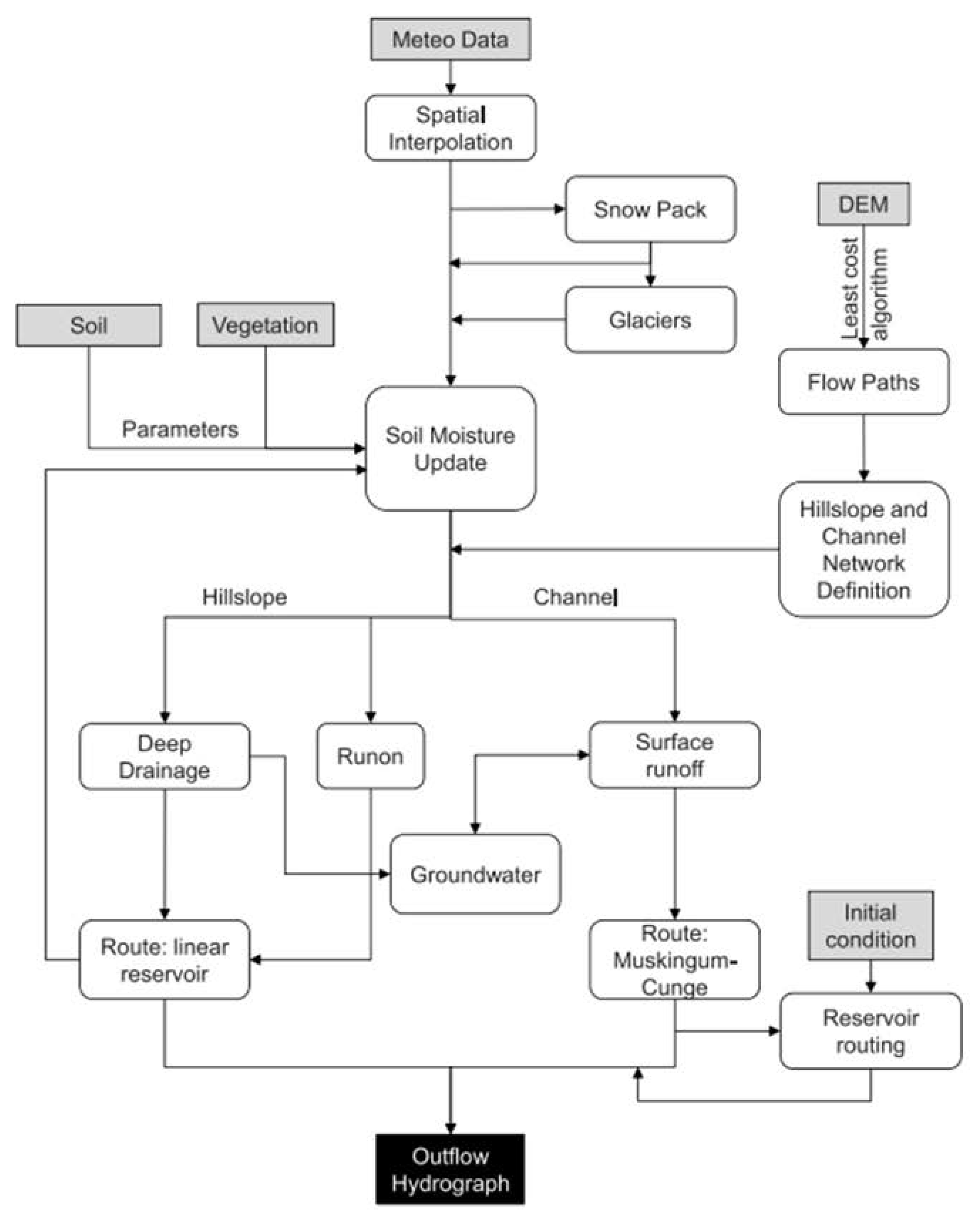
2.1.1. FEST-WB Distributed Hydrological Model

The potential evapotranspiration was computed according to the Priestley and Taylor model [29]. Within the FEST-WB model several options for the calculation of infiltration are implemented (modified SCS-CN (US Department of Agriculture Soil Conservation Service [30], in its differential form [31], Philip equation [32], and Green and Ampt [33]. More details are reported in [34].

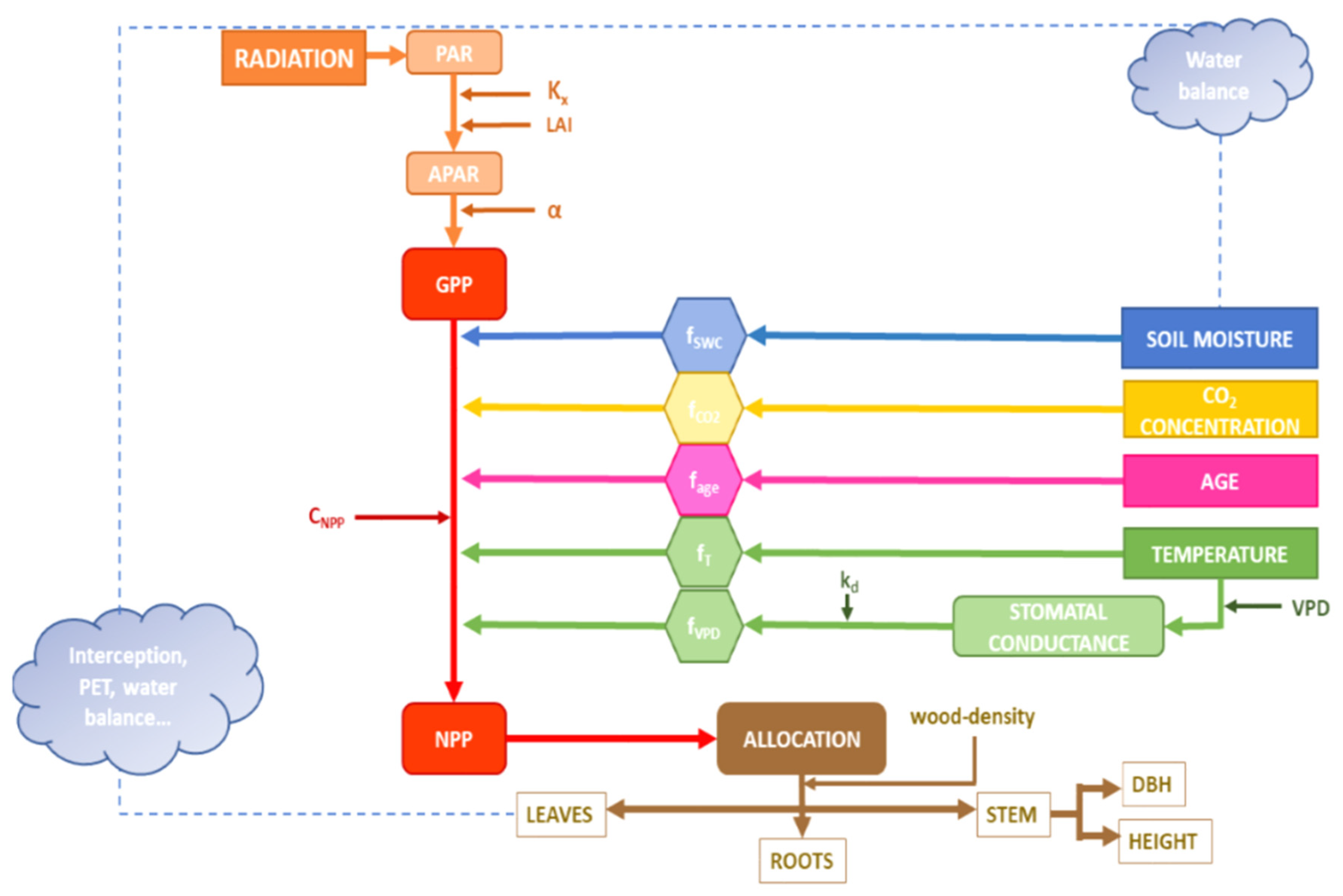
2.1.2. FOREST Module

The module was inspired by several existing eco-hydrological models and extensive research into the existing literature of the used equations to simulate vegetation growth and dynamic processes. Figure 2 displays main processes integrated in this model to simulate the forest growth. The model was developed using the FORTRAN 90 programming language. This was later developed considering one species per cell only and all the trees within each cell having the same characteristics. This choice was taken in order to simplify the process simulations and reduce the required inputs (considering also that for the area where this model will be used, 90% of the forest is covered with the same species).

• Light Interception

The amount of light available for the plant is going to define its growth rate and, together with other factors that may limit the plant growth, will be later taken into consideration. The light the plant could absorb is determined according to canopy cover. The amount of absorbed photosynthetically active radiation (APAR) is defined following the Lambert–Beer law [35], where:

$$APAR=PAR\times \left(1-ex{p}^{-K_{x}LAI}\right)$$

(1)

where PAR is the photosynthetically active radiation. Kx is the extinction coefficient for absorption of PAR by canopy, and varies between (0–1). This parameter is specific to each plant species, depending on the foliage transmissivity and leaves inclination; the LAI corresponds to the leaf area index (m² m⁻²).

The PAR can be calculated using the following formula:

$$PAR=\left(1-\alpha \right)\times Hday$$

(2)

where Hday is the short-wave solar radiation and α is the albedo. According to several studies, the short-wave solar radiation can be calculated as 50% of the APAR. These calculations are based on the assumption that the foliage is uniformly distributed. The radiation that was not intercepted by any of the vegetation crowns is going to reach the ground.

• GPP and NPP Calculation

The amount of carbon is defined through the intercepted radiation by the canopy (previously computed). Carbon assimilation is constrained by several factors such as temperature, water content, vapor pressure deficit.

These factors are called modifiers. For each class the GPP is calculated by the absorbed radiation and ε (gDM MJ⁻¹) the potential radiation use efficiency or maximum quantum canopy efficiency (α μmol CO₂ μmol⁻¹ PAR). The GPP for each class is calculated according to the following formula:

$$GP{P}_x={\epsilon }_x\times APA{R}_x\times Modifier{s}_x$$

(3)

The GPP (g cm⁻² month⁻¹) is calculated for each cohort. The maximum quantum canopy efficiency is species specific.

GPP should be adjusted to net primary production NPP (g cm⁻² month⁻¹) through a constant conversion factor C_NPP:

$$NPP=GPP\times C_{NPP}$$

(4)

Landsberg and Waring [13] found that C_NPP value for wide range of forests is about 0.47 ± 0.04.

• Modifiers Calculation

Increased availability of detailed forest inventory data supported the development of complex systems of differential or difference equations that simultaneously modeled change in individual components of stand growth [36,37], including ingrowth, growth of surviving trees, mortality, and harvest.

Several factors may affect the carbon allocation in forest ecosystem. This later is subject to the effect of vapor pressure deficit, soil water deficit, temperature (or frost) and the age of the trees.

• Soil water modifier

The soil water modifier (f_swcθ) implemented within the FEST-FOREST model is calculated according to the formula proposed by Cox et al. [38].

$$f_{swc}=\frac{1-e^{\left(\beta \times swc\right)}}{1-e^{\left(\phi \right)}}$$

(5)

$$f_{swc}=\frac{1-e^{\left(\beta \times {\phi }_{\theta }\right)}}{1-e^{\left(-{\phi }_{\theta }\right)}}$$

(6)

The empirical parameter to compute soil water content modifier function, and β is calculated as follows:

$$\beta =\{\begin{array}{c}0 \mathrm{for} \mathit{swc}<\mathit{WP}\\ \frac{swc-WP}{FC-WP} \mathrm{for} \mathit{WP}<\mathit{swc}<\mathit{FC}\\ 1 \mathrm{for} \mathit{swc}>\mathit{FC}\end{array}$$

(7)

2.

Temperature modifier

Temperature is considered as a limiting factor for the growth of vegetation when it is not within an optimum range. The growth and dormant stages of vegetation are related to the annual cycle of air temperature. Maximum growth will happen at optimal temperatures T_opt and will stop when temperatures drop below or exceed certain temperature thresholds, T_min and T_max, respectively. The temperature modifier is computed as follows:

$$f_T=\left(\frac{T_a-T_{min}}{T_{opt}-T_{min}}\right){\left(\frac{T_{max}-T_a}{T_{max}-T_{opt}}\right)}^{\left(T_{max}-T_{opt}\right)/\left(T_{opt}-T_{min}\right)}$$

(8)

Ta is the air temperature, T_min is the minimum temperature for the plant growth, T_max is the maximum temperature for the plant, and T_opt is the optimum temperature for the plant growth. This modifier was implemented according to the temperature modifier as proposed by Landsberg and Waring [13].

• Age modifier

The vegetation age is considered based on the factors that may affect the carbon allocation. The trees in the early stages are not growing as faster as mature trees. The age modifier is computed following Peng et al. [39].

if age < 0.2 age_max

$$f_{age}=0.7+0.3\frac{age}{0.2ag{e}_{max}}$$

(9)

Otherwise

$$f_{age}=1+max\left[0, {\left(\frac{age-0.2ag{e}_{max}}{0.95ag{e}_{max}}\right)}^3\right]$$

(10)

where age is the effective age of the vegetation, age_max is the maximum age that the tree can achieve.

3.

Vapor pressure modifier (Landsberg and waring-3PG)

The vapor pressure modifier (implemented according to Landsberg and Waring- 3PG model) is calculated with the following formula:

$$f_{VPD}=exp\left(-k_{g}D\right)$$

(11)

with f_VPD vapor pressure modifier, kg empirical coefficient describing the relationship between stomatal and canopy conductance and D average vapor pressure deficit. The vapor pressure deficit is computed according to Dingman [40]:

$$ESTAR=6.1076\times e^{\left(\frac{17.269\times T_a}{T_a+237.3}\right)}$$

(12)

with ESTAR is the saturation vapor pressure of the air [mbar], and T_a is the actual air temperature [°C].

4.

CO₂ modifier

The last modifier considered is the one relating to CO₂ concentration in atmosphere. In fact, the presence of carbon dioxide in the atmosphere is vital to plants in order to activate the photosynthesis processes.

The CO₂ modifier f_CO2 is implemented according to the following formula [15]:

$$f_{C{O}_2}=\frac{f_{C\alpha x}·C{O}_2}{350·\left(f_{C\alpha x}-1\right)+C{O}_2}$$

(13)

where f_Cαx is a dimensionless parameter to compute the modifier, and CO₂ is the current carbon dioxide concentration [ppm] in the atmosphere.

• Carbon Allocation

The model allows to simulate the carbon allocation to roots, stem, and foliage. This step will permit to follow the forest change in subsequent years according to the value of NPP previously calculated. The increments in roots (ΔMroot), stem (ΔMstem), and foliage (ΔMleaf) are calculated as follows [13]:

$$\mathsf{\Delta }{M}_{root}=NPP\times {\eta }_r$$

(14)

$$\mathsf{\Delta }{M}_{stem}=NPP\times {\eta }_s$$

(15)

$$\mathsf{\Delta }{M}_{leaf}=NPP\times {\eta }_f$$

(16)

where η_r, η_s, and η_f are the partitioning factors to allocate NPP to roots, stem, and leaves respectively. The allocation is based on an assumption made by Landsberg and Waring [13] that the plant will allocate more carbon to root rather than to stem under resources shortages. These partitioning factors are calculated as follows:

$${\eta }_r=\frac{0.5}{1+2.5\times f_{age}{f}_T{f}_{\theta }}$$

(17)

$${\eta }_s=\frac{1-{\eta }_r}{1+p_{fs}}$$

(18)

and

$${\eta }_f=1-{\eta }_r-{\eta }_s$$

(19)

where p_fs is a partition function dependent on species-specific parameters:

$$p_{fs}=\frac{F_{prn}\times F_{pra}}{S_{prn}\times S_{pra}} DB{H}^{\left(F_{prn}-S_{prn}\right)}$$

(20)

with F_prn, F_pra, S_prn, and S_pra are vegetation dependent empirical parameters and DBH is the total diameter at breast height of the sum of the individual trees of species in the pixel.

After the carbon allocation, the model updates the value of LAI, root mass, and the size of the trees. The increment in the LAI is function of the carbon allocated to foliage and leaf turnover due water and temperature stresses. The LAI corresponds to the gross leaf production that should be updated according to the value of leaf turnover computed as follow:

$$\mathsf{\Delta }LAI=\sigma LAI\times \mathsf{\Delta }Mleaf-\left({\delta }_f+{\delta }_{fw}+{\delta }_{ft}\right)\mathsf{\Delta }t\times LAI$$

(21)

where σLAI is a specific leaf area index (m²g⁻¹) of a vegetation, δ_f is a constant leaf turnover rate for a vegetation type p, δ_fw, and δ_ft are foliage loss coefficients due to hydrologic and temperature stresses and ∆t is time step (s).

The foliage loss is mainly due to the water and temperature stresses:

$${{\delta }_{fw}}_p={{\delta }_{fw}}_{\left(p\right)max}{\left(1-{\beta }_{\delta w\left(p\right)}\right)}^{\gamma \delta w\left(p\right)}$$

(22)

$${{\delta }_{fT}}_p={{\delta }_{fw}}_{\left(T\right)max}{\left(1-{\beta }_{\delta T\left(p\right)}\right)}^{\gamma \delta T\left(p\right)}$$

(23)

where δ_fw(p)max and δ_fw(T)max are maximum leaf decay rates (s⁻¹) due to water and temperature factors, respectively, and γδw(p) and γδT(p) are dimensionless shape parameters.

With water stress expressed by:

$${\beta }_{\delta w\left(p\right)}=max\left[0, \min (1, \left(\theta -{\theta }_{FC}\right)/\left(\theta -{\theta }_{FC}\right)\right]$$

(24)

The temperature stress is expressed by:

$${\beta }_{\delta T\left(p\right)}=max\left[0, \min (1, \frac{(T_a-\left(T_{cold}-5\right)}{5}\right]$$

(25)

The roots increment is computed by:

$$\mathsf{\Delta }root{s}_p=\mathsf{\Delta }{M}_{root\left(p\right)}-\delta r_{\left(p\right)}\times \mathsf{\Delta }t\times Roo{t}_{\left(p\right)}$$

(26)

where Root root is the root mass (Kg m⁻²) and δr_(p) is the base root turnover rate (s⁻¹).

The tree height and diameter increments are

For $cc\le 0.95$

$$H{D}_{eff}=H{D}_{min}+\left(H{D}_{max}-H{D}_{min}\right)\ast cc$$

(27)

else

$$H{D}_{eff}=H{D}_{max}$$

(28)

where the height increment is computed as follows:

$$dheight=\frac{H{D}_{eff}}{\frac{H{D}_{eff}}{height}+\frac{200}{DBH}}\times \frac{dws}{WS}$$

(29)

The tree diameter increment is calculated:

$$dDBH=\frac{height}{H{D}_{eff}}+\frac{200}{DBH}\times \frac{dws}{WS}$$

(30)

where cc stands for the canopy cover. This parameter value ranges between 0 and 1. This parameter is computed according to crown diameter and trees density.

The tree height and diameter is afterwards updated according to the previously calculated increments:

$$DBH=DBH+dDBH$$

(31)

$$height=height+dheight$$

(32)

• Total Biomass Calculation

The biomass of root, stem and foliage is updated considering the initial values of these latter. The total biomass is equal to:

$$bi{o}_{tot}=M_{roots}+M_{stem}+M_{foliage}$$

(33)

• Mortality

In the FEST-FOREST three types of factors that induce trees mortality were considered:

-

The first mortality factor is due to the self-thinning (the one included in 3PG), which ensures that the mean single-tree stem biomass WS does not exceed the maximum permissible single-tree stem biomass WSx [kg·tree⁻¹] [41].

-

The second mortality factor is age dependent mortality following the approach of LPJ-GUESS (SMITH) [42] with aging the plants become more susceptible to the wind, diseases, etc.

-

The third mortality factor is the so called the “crowding competition function”, this mortality ensures that the % of cover of pixel does not exceed 95%.

After calculating the mortality, the biomass allocated to roots, stems and foliage is updated according to the following formulas:

$$WF=WF-mF \ast delStems \ast \left(WF / density\right)$$

(34)

$$Wr=Wr-mr \ast delStems \ast \left(Wr / density\right)$$

(35)

$$Ws=Ws-ms \ast delStems \ast \left(Ws / density\right)$$

(36)

where mF, mr and ms (mean foliage, roots, and stems) are the fractions of the biomass pools per tree of each dying tree

$$delStems=density-Densit{y}_{after}$$

(37)

in which delStems refers to the number of dead trees, density is the total number of trees and Density_after is the number of trees after removing the dead ones.

• Management Options

The stand biomass C is directly influenced by several factors as rotation length, frequency, and intensity of thinning, other disturbances. A module which considers different forest management options was inserted allowing to simulate the forest growth under different managements selected by the user. As of today, it is not possible to simulate in the same stand plants with different age; for this reason, the number of management options in this version were limited. The management options are the following:

Thinning: it is possible to choose the intensity of the thinning in terms of percentage from the total number of the trees as well as the interval of thinning (years).

Rotation: Clear-cut option in which it is possible to remove completely the plants and plant new trees with a certain rotation interval that the user can choose.

2.2. Model Application

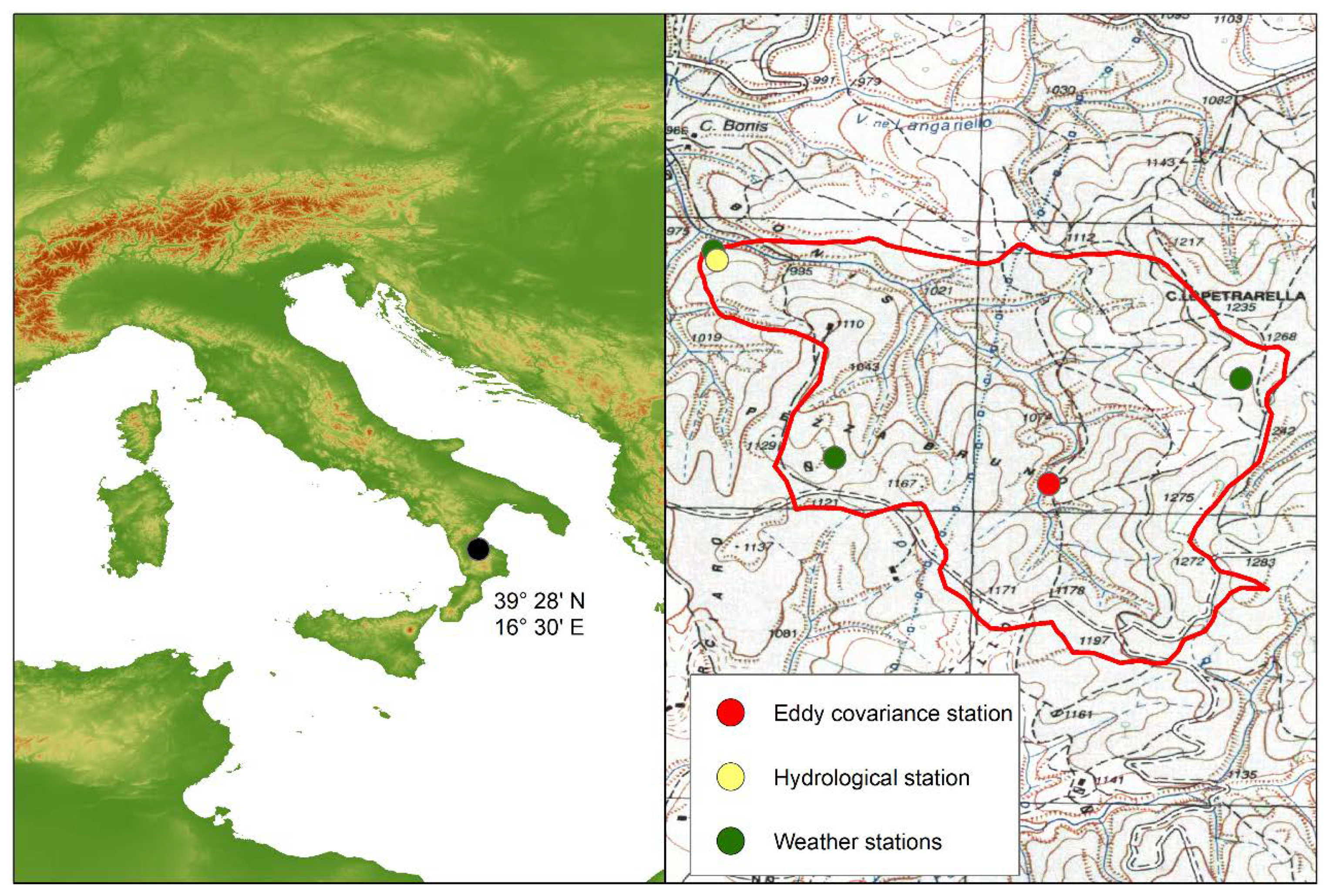
2.2.1. Study Catchment Data

The Bonis catchment (Figure 3) is located (39°25′15″ N, 16°12′38″ W) in the mountain area of the Calabria region (southern Italy). In particular, it covers an area of 1.39 km² of the Sila Plateau (1500 km²) with a mean elevation of 1131 m above sea level. The catchment is underlain by acid plutonic rocks [43] characterized as Typic Xerumbrepts and Ulpic Haploxeralfs [44]. The forest and rangeland cover around 93% of the total area of the basin, dominated by about 50–60-year-old Calabrian pine (Pinus laricio Poiret). A selective thinning was carried out in 1993, which reduced the stands density by around 55% (38% in low-density stands, 69% in high-density stands). Since 1986 the basin was monitored through the installation of different instruments. Rainfall was measured by three rain gauges (with a tipping bucket), together with temperature measured at three different meteorological stations located at the basin outlet (Outlet: 975 m above sea level a.s.l.) and at representative sites within the north-eastern (Petrarella: 1258 m a.s.l.) and southwestern (Don Bruno: 1175 m a.s.l.) parts of the catchment. Runoff was measured at the outlet of the catchment using a gauging structure. In May 2003, a tower for measurement of eddy fluxes was installed at an altitude of 1100 m a.s.l, on a 54-year-old plantation of Laricio pine which allowed the monitoring of other parameters. Although the monitoring period is considered quite long, during the analysis of the collected data (in particular the hourly data), some inhomogeneity of data series and missing data were found because of occasional interruptions in automatic recorders and instrumentation failure [44]. For the missing meteorological data, measurements of the closest meteorological station were used, which in our case is the Cecita station (39°23′1.26″ N, 16°32′55.01″ E) located a few kilometers from the Bonis catchment and managed by the Multi-Risk Functional Centre of the Regional Agency for Environment Protection of the Calabria Region. The climate is typical of the mountain areas of Calabria, characterized by an average recorded annual precipitation of 915 mm; the mean temperature of the coldest month is about 0.1 °C and of the hottest month is 18.3 °C [45]. Dendrological measurements were also carried out through field surveys at this basin, before and after the forest thinning in 1993. These measures allowed to reconstruct the history of the forest at this catchment [46].

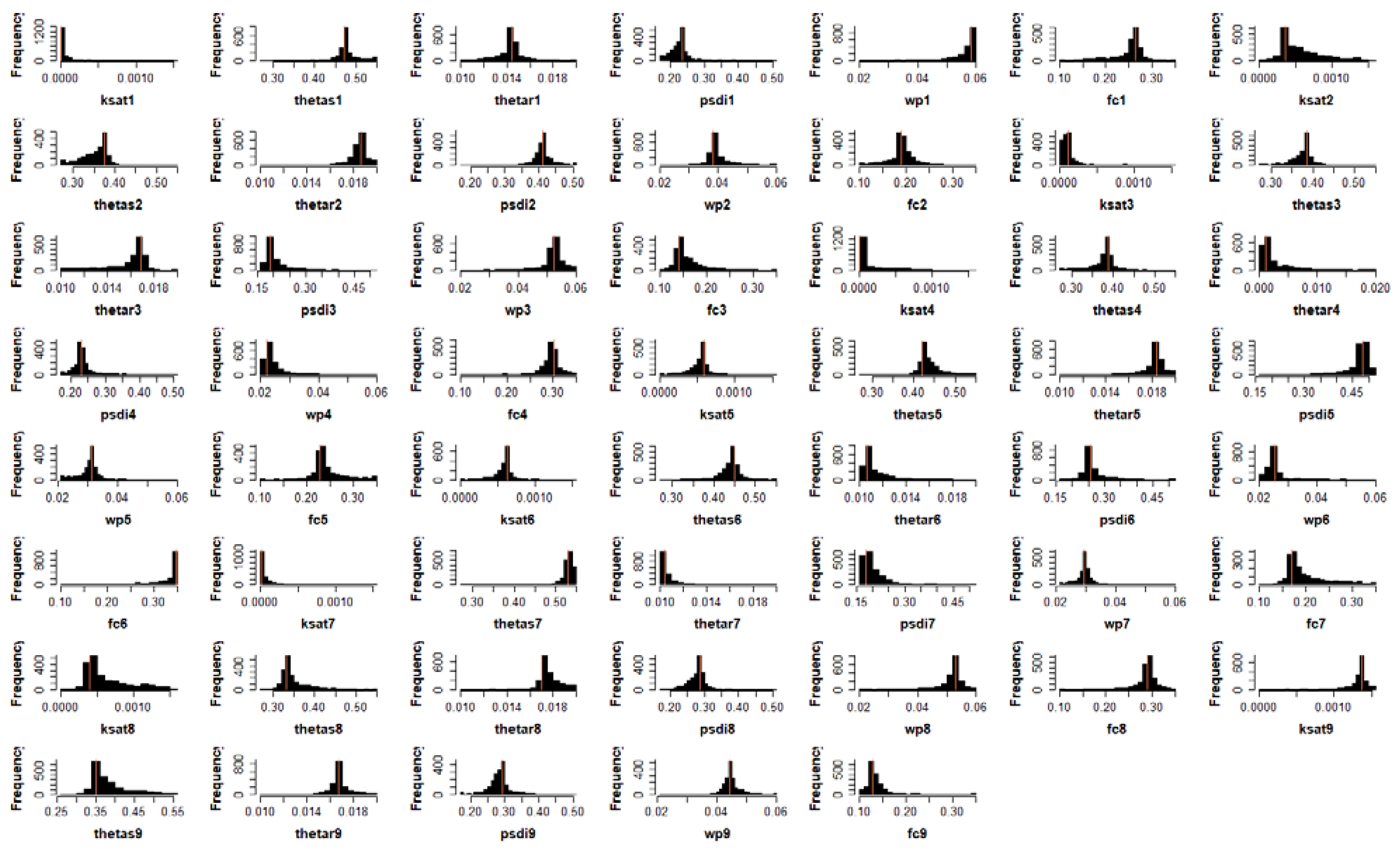
2.2.2. Soil Parameters

Soil data were determined through field and laboratory measurements. Field measurements were carried out following the Beerkan Estimation of Soil Transfer parameters (BEST) method [47]. This method allows to estimate soil hydraulic properties from basic soil properties together with infiltration measurements. Disturbed soil samples were collected in order to determine the particle size distribution performed by sieving for sand fraction for each soil. For the analysis of the finer part, an automated particle size distribution instrument (METER Group, München, Germany) was used. Sand, silt, and clay contents together with soil texture were identified according to the USDA (United States Department of Agriculture) system of soil classification. The topsoil of the Bonis catchment was classified, according to the different fractions of sand, clay, and loam, and Loamy fine sand for the majority of sampling locations, while others were characterized by a fine sand soil. For this study the average of the measured soil parameters was considered as representative for the entire catchment.

Measured soil parameters at different land uses of the catchment were used as a first estimate to be subsequently calibrated. These parameters were also used to assess the contribution of each land use to hydrological response of the basin. The sampling points were selected as representative of the mainland uses of the basin. In order to simplify the data collection, similar land uses were gathered under the same land use category. This procedure generated a second simplified classification with 9 different land use classes instead of 16 as reported in the

Table 1. Different land covers and corresponding surface area of Bonis catchment.

ID	Land Cover	Surface
		(km2)
1	Artificial Laricio pine forests with Turkey Oak in subcanopy layer	0.3872
2	Low density of artificial Laricio pine forests	0.0444
3	Artificial Laricio pine degraded forests	0.1108
4	Natural and artificial Laricio pine forests (low density)	0.258
5	Natural Laricio pine forests (high density)	0.08
6	Artificial Laricio pine forests crossed by fire	0.0256
7	Chestnut coppice, Alder and poplar riparian forests, Artificial chestnut forests and mixed Laricio pine and Chestnut forests	0.3748
8	arable land	0.0232
9	bare soil and outcropping rocks	0.0772

.

2.2.3. Model Calibration

After the model set up and initialization with measured soil data, the HydroPSO—a model independent R package based on particle swarm optimization algorithm developed by Rojas and Zambrano-Bigiarini [48]—was used for the calibration. The HydroPSO can be coupled with any hydrological model. This latter was also used to carry the sensitivity analysis of the model. In order to couple the HydroPSO with the FEST-WB, minimal modeling efforts were required to exchange inputs and outputs of the simulations.

Three text files were prepared. The first contains the list of parameters, to be calibrated and their locations in the model input files); the second defines the range of variability of parameters and the last text file contains the observations (hourly runoff discharges for this study). The interface between the HydroPSO and the FEST-WB, requires two R wrapper functions to read the model output and the observations required for the calculation of the goodness of fit function (GoF). Several GoFs are implemented in the HydroPSO such as: Root Mean Square Error (RMSE), Normalized RMS (NRMSE), Pearson correlation coefficient (r), coefficient of determination (R2), modified NSE (mNSE), index of agreement (d), coefficient of persistence (cp), percent bias (pbias), and Kling-Gupta Efficiency (KGE) [48]. Details about all the functionalities implemented in the HydroPSO, are reported in the package documentation. The number of particles (swarm size) was set to 20 and as goodness of fit function the efficiency NSE was selected. NSE was proposed by Nash and Sutcliffe [49] varying between −∞ and 1.

The work was subdivided in two parts:

-

The hydrological part: sensitivity analysis and calibration using measured runoff data.

-

The forest growth part: sensitivity analysis and calibration using dendrological measurements.

3. Results

3.1. Hydrological Simulations

3.1.1. Sensitivity Analysis

Sensitivity analysis was carried out to test the sensitivity of runoff simulations to the soil data input parameters. Following the proposed methodology, the sensitivity analysis was performed using the “lhoat()” function incorporated in the HydroPSO package that uses the Nash–Sutcliffe efficiency (NSE) as measure of model performance. The sensitivity analysis was carried out using observed discharge time series. The results are reported in the

Table 2. Sensitive parameter ranking of each of tested infiltration method.

Ranking	Parameters
1	Saturated water content: θs
2	Particle size distribution index: psdi
3	Saturated hydraulic conductivity: ksat
4	Water content at field capacity: fc
5	Water content at wilting point: wp
6	Residual water content: θr

, where only the ranking of sensitive parameters are presented. This step allowed to reduce the number of parameters to be calibrated using the HydroPSO where only sensitive parameters were considered for the runoff simulations.

3.1.2. Runoff Simulations Calibration

Short simulation periods were taken into account in order to consider the vegetation as static. For the calibration of the runoff simulations, distributed soil parameters were considered according to the different land uses. Green and Ampt model was selected for the simulation of the infiltration process. After several iterations, the automatic calibration allowed to minimize the error between the measured and simulated surface runoff. The use of such automatic calibration allowed to reduce the computation time.

Although not shown here because beyond the scope of this paper, several trials with different swarm sizes, and goodness of fit functions with different number of iterations were tested including different numbers of iterations, swarm sizes and boundary conditions. Figure 4 presents the histogram of calibrated values. The vertical red line highlights the optimum value achieved by each parameter. These histograms show near normal distribution or skewed distribution near to the upper boundary.

The calibration is based on the optimization of a goodness of fit function, in this case the Nash-Sutcliffe Efficiency was selected. Figure 5 reports the evolution of the GoF as a function of the iteration number. At the end of the calibration, the GoF reached a value equal to 0.88 which refers to a good match between the observations and calibration results.

In order to better analyze these simulations, several short simulation periods were selected as reported in

Table 3. Selected simulation periods for the calibration and validation.

Simulation Period	Start	End
C1	8 September 2001	30 December 2002	Calibration
C2	16 January 1986	28 February 1986
C3	1 January 1988	5 October 1989
C4	31 January 1990	17 August 1991
C5	18 November 1991	1 October 1992
V1	21 June 2018	22 June 2018	Validation
V2	25 June 2018	29 June 2018
V3	4 October 2018	5 October 2018
V4	23 October 2018	24 October 2018

.

In Figure 6 results of the automatic calibration were compared with measured runoff volumes. The performance of the calibration varies from one simulation period to another, but as an overall calibration outcome, satisfactory results were achieved.

In addition, the validation of the calibration results was carried out by selecting some rainfall events. Some of the events selected are reported in Figure 7. As shown in the figure, the calibration allowed to improve the simulation results, reaching different levels of accuracy according to different selected events.

3.2. Forest Growth Simulations

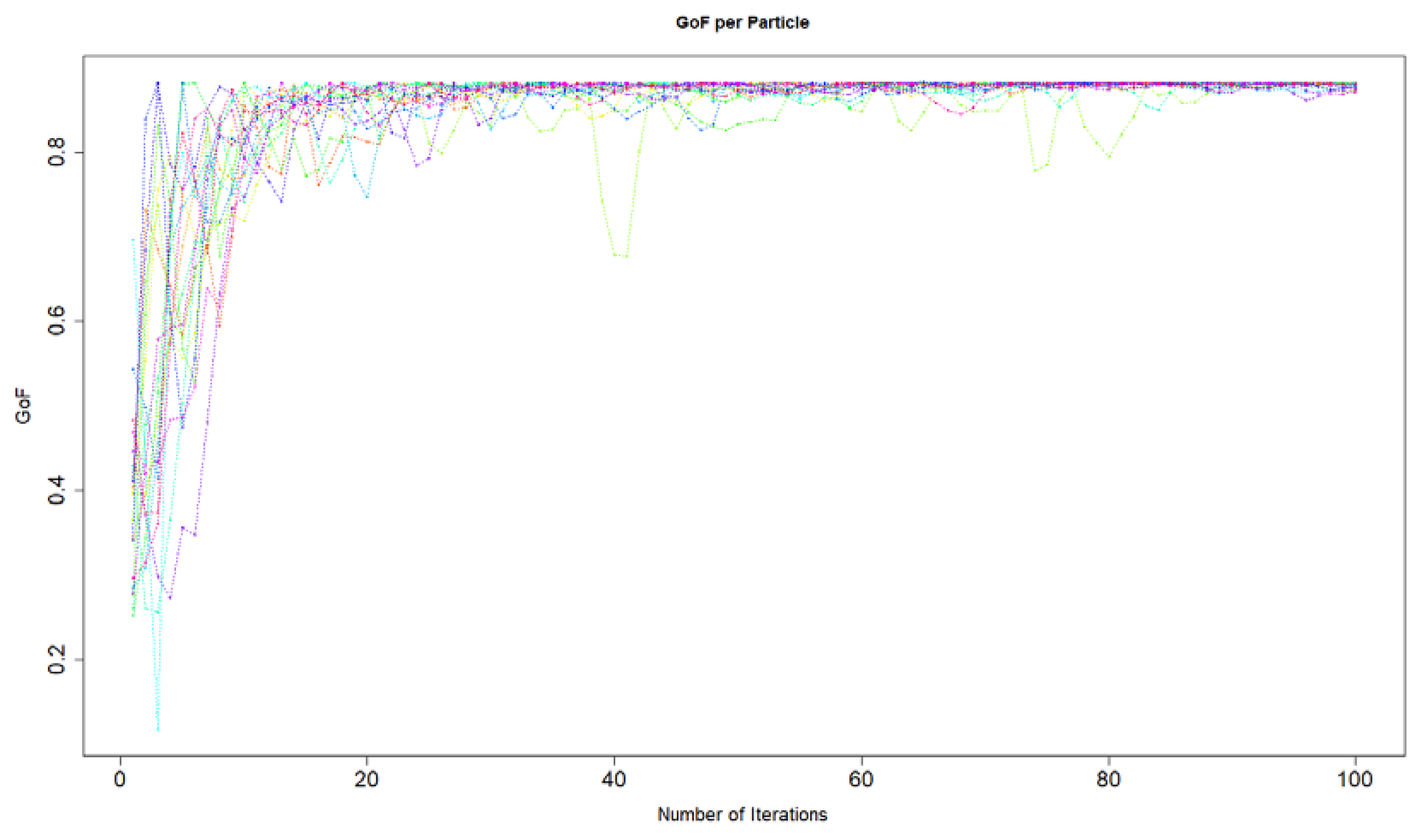
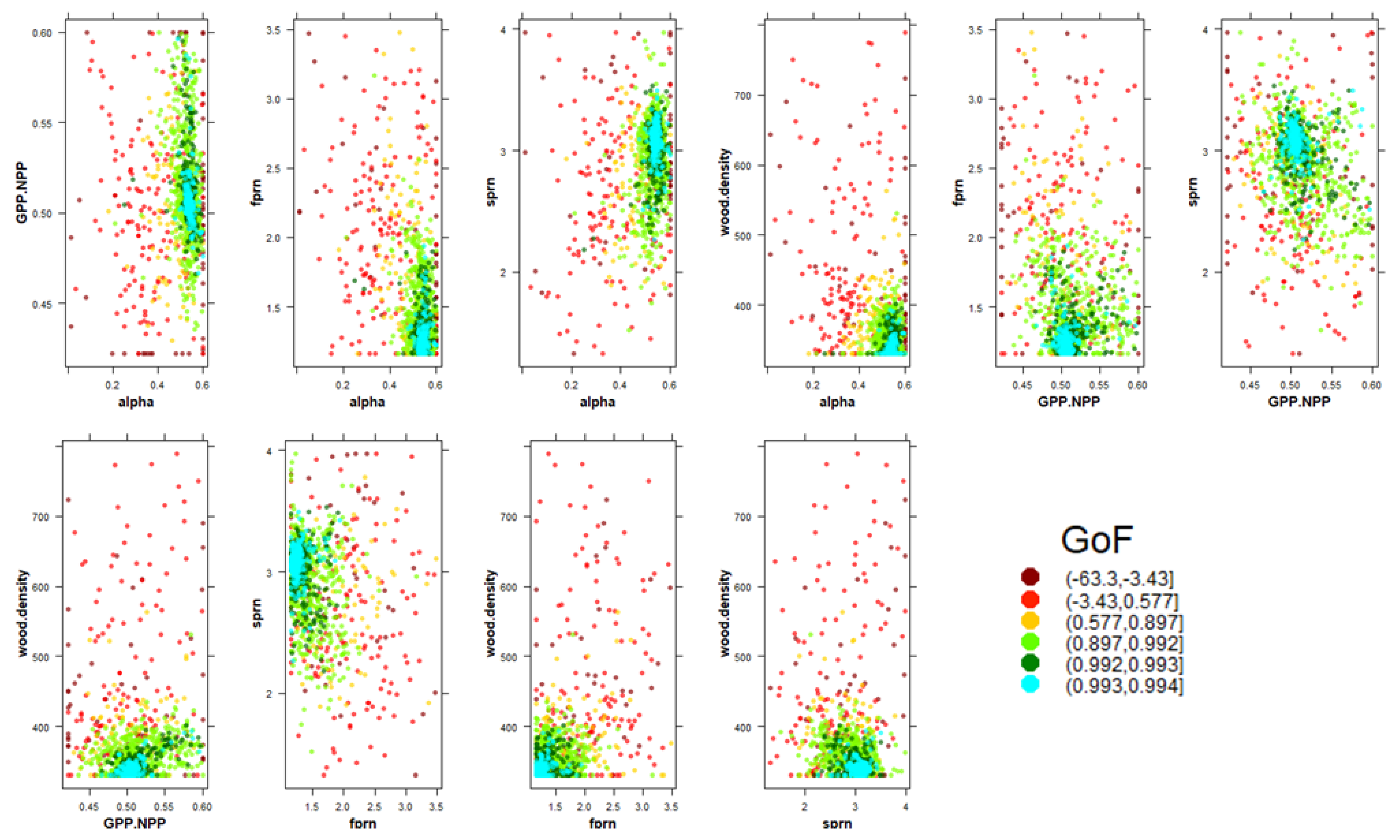
3.2.1. Sensitivity Analysis

The ranges of variability of the parameters have been mainly selected from literature. For some parameters the ranges have been fixed as p ± 50%, where p is the starting value of the parameters, whereas other parameters’ variability was taken according to the literature. Results of the sensitivity analysis of the FEST-FOREST model input parameters are presented in

Table 4. Importance ranking obtained with the sensitivity analysis.

Ranking Number	Parameter Name	Relative Importance Norm
1	fprn: Parameter to compute allocation factors	5.32 × 10−1
2	Sprn: Parameter to compute allocation factors	2.58 × 10−1
3	GPP-NPP: GPP/NPP ratio	4.53 × 10−2
4	Alpha: Parameter to compute allocation factors	3.88 × 10−2
5	wood-density	3.57 × 10−2
6	agemax: maximum age of the plant	2.01 × 10−2
7	hdmin: H/D ratio in carbon partitioning for low density	1.40 × 10−2
8	phi-theta: Empirical coefficient of the soil moisture efficiencyfunction for canopy resistance	1.15 × 10−2
9	k: H/D ratio in carbon partitioning for low density	1.04 × 10−2
10	albedo: Plant albedo	8.76 × 10−3
11	fpra: Parameter to compute allocation factors	7.45 × 10−3
12	Spra: Parameter to compute allocation factors	7.43 × 10−3
13	Sla: Specific leaf area	2.92 × 10−3
14	phi-ea: Empirical coefficient of the vapor pressure efficiency function for canopy resistance	2.71 × 10−3
15	canopymax: maximum canopy storage capacity	2.20 × 10−3
16	laimax: maximum leaf area index used for precipitation interception	2.00 × 10−3
17	hdmax: H/D ratio in carbon partitioning for low density	4.41 × 10−4
18	tcold-leaf: Temperature threshold that accelerates leaf turnover	1.67 × 10−4
19	dbhdcmax: maximum ratio between stem and crown diameters	3.42 × 109
20	dbhdcmin: minimum ratio between stem and crown diameters	2.79 × 109
21	denmax: maximum trees density	1.67 × 109
22	denmin: minimum trees density	5.48 × 107

. The parameters are ranked starting from the most to the least sensitive.

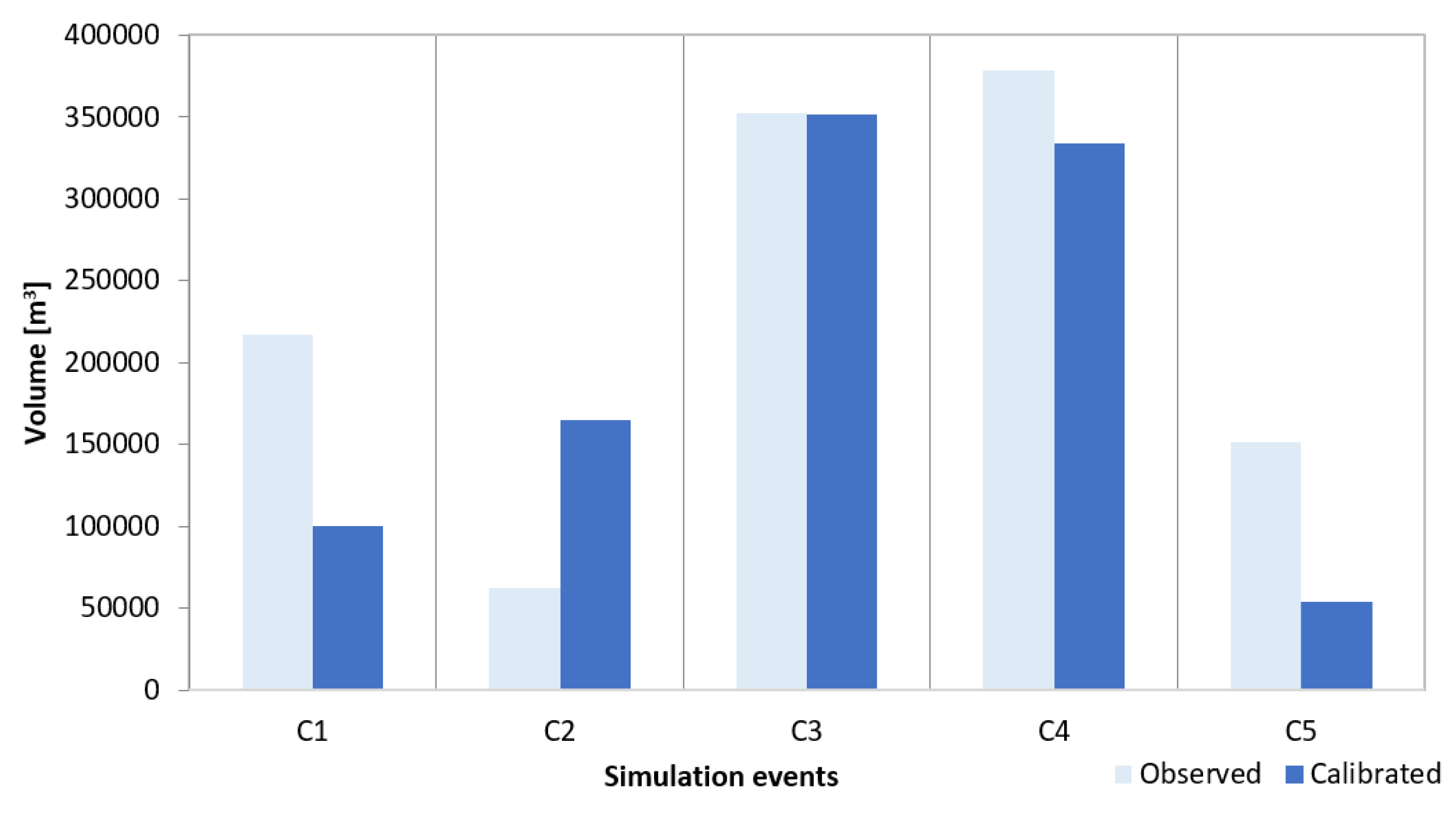
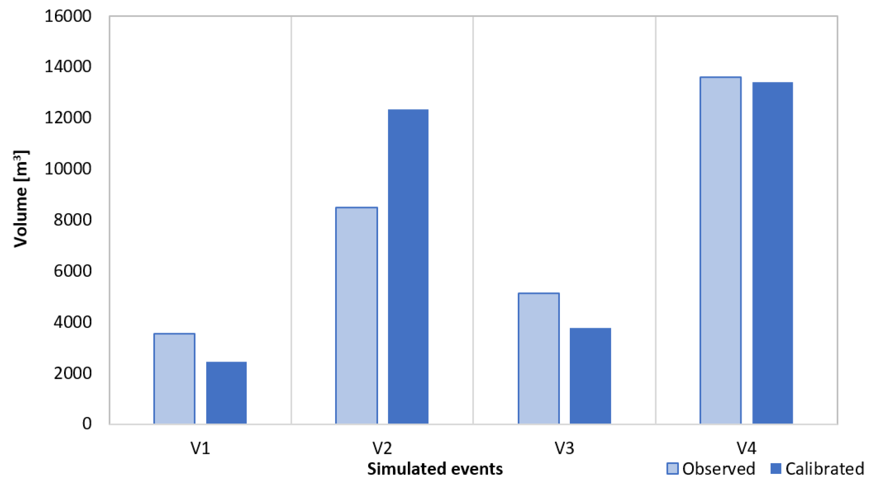
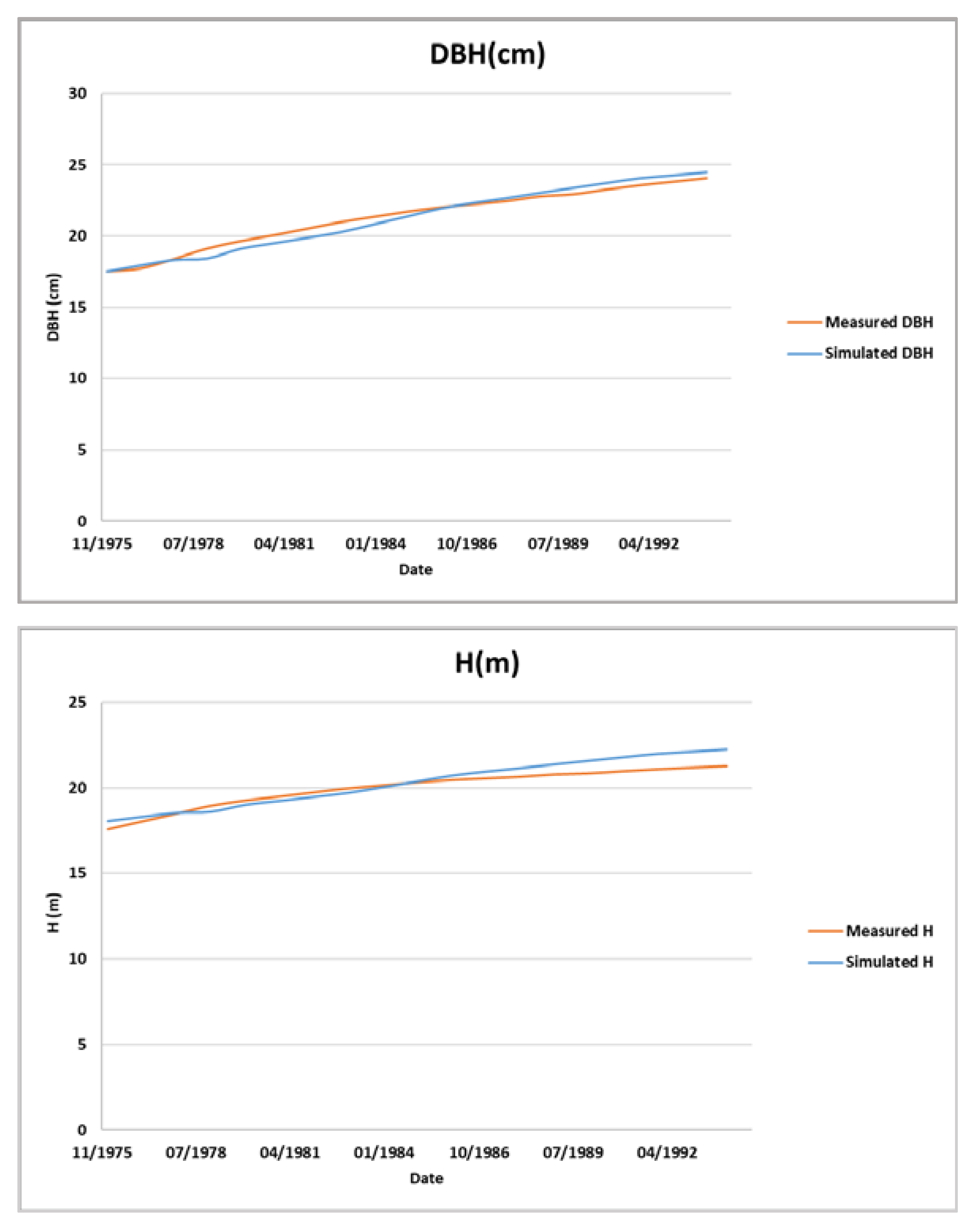
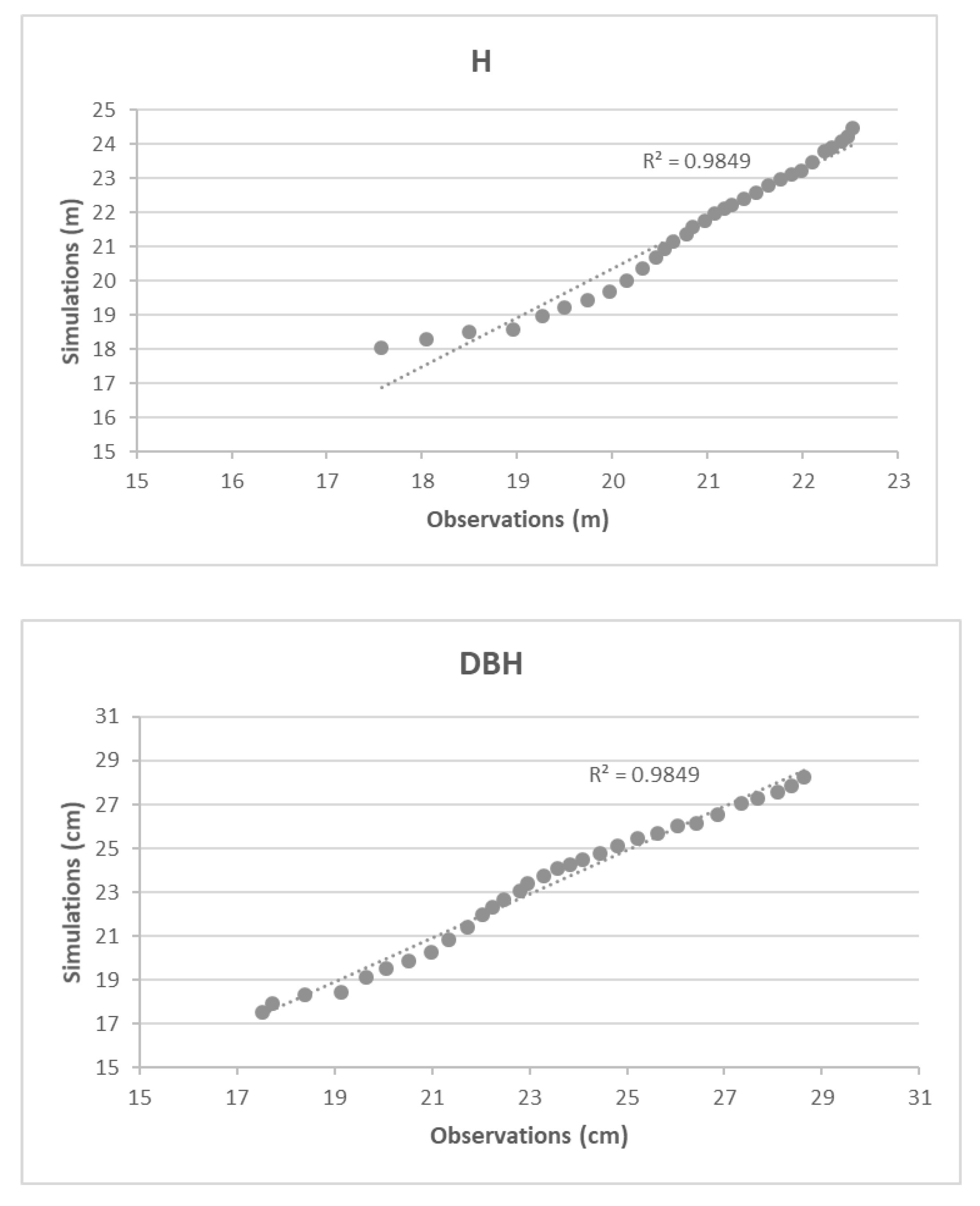
3.2.2. Model Calibration Forest Growth Simulations

For the model calibration as a first step the Hydro-PSO model was used, introducing a range of variability for the most sensitive parameters. The number of parameters to be calibrated was reduced according to the results of the sensitivity analysis. The selected parameters for the calibration were limited to the first five parameters. Other parameters were set as constant during this calibration phase.

The calibration was carried out using measured data from Bonis catchment: H which is the height and DBH which is the diameter at the breast height. In order to reach better simulation results for both DBH and H, calibrated parameters issued from these two calibrations were combined. All simulations were carried out with daily time steps. Initialization of the model was performed using measured data. The model calculated the increment of the biomass of each tree component.

Figure 8 presents a 2D projection of the goodness-of-fit (NSE) surface response for different parameter pairs. The particles tend to converge in the light-blue areas, where NSE reaches its maximum values.

After a combination of manual and automatic calibration of parameters, good performances were reached with regards to the simulation of DBH and H.

Figure 9 and Figure 10 report the results of calibration as compared to measured data. For DBH simulation the coefficient of determination was equal to 0.98 between simulation and observations while for the H was equal to 0.96.

The model was calibrated for both hydrological and forest growth simulations. Results of both simulations proved that the ability of the FEST-WB integrated with the FOREST module could be implemented to study both processes in a reliable way. The model at a first step was calibrated for the hydrological part. Subsequently, the calibration of forest growth was carried out. Both processes are interconnected through many parameters such as soil water content, water and light interception, and evapotranspiration. Simulation results reflect the ability of the model as a whole and through the integration of hydrological and forest growth to reproduce an accurate response of the catchment to eco-hydrological dynamics.

A similar study was carried out by Pellicone [46] in the same area, in which the 3D-CMCC-CNR model was calibrated and validated against forest growth measurements, and without any consideration of hydrological data. The performances reached using this model are comparable to the results of the newly developed FOREST module integrated in FEST-WB model that, in addition to the 3D-CMCC-CNR model, can properly simulate the hydrological components. FEST-FOREST model is considered as sophisticated model, similarly to some existing models such as SWAT, with the difference that FEST-FOREST model is fully distributed simulated.

4. Conclusions

The main purpose of this paper was to present the recently developed model FEST-FOREST. This derives by inclusion of the newly developed FOREST module within the FEST-WB distributed hydrological model. The development of the new module was based on extensive literature review. The selection of the equations used for the simulation of different processes related to forest growth targeted mainly the availability of the required input parameters. The FEST-FOREST was used to simulate the forest dynamics for a study site located in the south of Italy, Bonis catchment.

The novelty of this paper is that existing eco-hydrological models usually simplify either the hydrological component or the forest growth component. The presented model is considered to be a sophisticated distributed hydrological model, which in its new release, allows to simulate the forest growth component and its interactions with the hydrological cycle. The model simulation results are very promising. Future applications of the FEST-FOREST model will allow to catch the response of forest growth to different meteorological scenarios and/or management scenarios together with the impact on the hydrological response of the catchment. Forthcoming improvements of the model are among our targets in order to get more realistic and accurate simulation results of the forest dynamics.

References

1. FAO; UNEP. The State of the World’s Forests 2020: Forests, Biodiversity and People; Food and Agriculture Organization of the United Nations: Rome, Italy, 2020. [Google Scholar]
2. Bradshaw, R.; Sykes, M. Ecosystem Dynamics: From the Past to the Future; John Wiley and Sons: Chichester, UK, 2014. [Google Scholar]
3. Bauhus, J.; van der Meer, P.; Kanninen, M. (Eds.) Ecosystem Goods and Services from Plantation Forests; Routledge: London, UK, 2010. [Google Scholar]
4. Thompson, I.D.; Okabe, K.; Tylianakis, J.M.; Kumar, P.; Brockerhoff, E.G.; Schellhorn, N.A.; Parrotta, J.A.; Nasi, R. Forest biodiversity and the delivery of ecosystem goods and services: Translating science into policy. Bio Sci. 2011, 61, 972–981. [Google Scholar] [CrossRef]
5. Brockerhoff, E.G.; Jactel, H.; Parrotta, J.A.; Ferraz, S.F. Role of eucalypt and other planted forests in biodiversity conservation and the provision of biodiversity-related ecosystem services. For. Ecol. Manag. 2013, 301, 43–50. [Google Scholar] [CrossRef]
6. Decocq, G.; Andrieu, E.; Brunet, J.; Chabrerie, O.; De Frenne, P.; De Smedt, P.; Deconchat, M.; Diekmann, M.; Ehrmann, S.; Giffard, B.; et al. Ecosystem services from small forest patches in agricultural landscapes. Curr. For. Rep. 2016, 2, 30–44. [Google Scholar] [CrossRef] [Green Version]
7. Liang, J.; Crowther, T.W.; Picard, N.; Wiser, S.; Zhou, M.; Alberti, G.; Schulze, E.-D.; McGuirei, A.D.; Bozzato, F.; Pretzsch, P.B.H.; et al. Positive biodiversity-productivity relationship predominant in global forests. Science 2016, 354, aaf8957. [Google Scholar] [CrossRef] [Green Version]
8. Mori, A.S.; Lertzman, K.P.; Gustafsson, L. Biodiversity and ecosystem services in forest ecosystems: A research agenda for applied forest ecology. J. Appl. Ecol. 2017, 54, 12–27. [Google Scholar] [CrossRef]
9. Pretzsch, H.; Grote, R.; Reineking, B.; Rötzer, T.; Seifert, S. Models for forest ecosystem management: A European perspective. Ann. Bot. 2008, 101, 1065–1087. [Google Scholar] [CrossRef]
10. Porté, A.; Bartelink, H.H. Modelling mixed forest growth: A review of models for forest management. Ecol. Modell. 2002, 150, 141–188. [Google Scholar] [CrossRef]
11. Dale, V.H.; Doyle, T.W.; Shugart, H.H. A comparison of tree growth models. Ecol Model. 1985, 29, 145–169. [Google Scholar] [CrossRef]
12. Zhou, B.Z.; Fu, M.Y.; Xie, J.Z.; Yang, X.S.; Li, Z.C. Ecological functions of bamboo forest: Research and application. J. For. Res. 2005, 16, 143–147. (In Chinese) [Google Scholar]
13. Landsberg, J.J.; Waring, R.H. A generalized model of forest productivity using simplified concepts of radiation-use efficiency, carbon balance and partitioning. For. Ecol. Manag. 1997, 95, 209–228. [Google Scholar] [CrossRef]
14. Landsberg, J.J.; Waring, R.H.; Coops, N.C. Performance of the forest productivity model 3-PG applied to a wide range of forest types. For. Ecol. Manag. 2003, 172, 199–214. [Google Scholar] [CrossRef]
15. Veroustraete, F.; Sabbe, H.; Eerens, H. Estimation of carbon mass fluxes over Europe using the C-Fix model and Euroflux data. Remote Sens. Environ. 2002, 83, 376–399. [Google Scholar] [CrossRef]
16. Sitch, S.; Smith, B.; Prentice, I.C.; Arneth, A.; Bondeau, A.; Cramer, W.; Kaplan, J.O.; Levis, S.; Lucht, W.; Sykes, M.T.; et al. Evaluation of ecosystem dynamics, plant geography and terrestrial carbon cycling in the LPJ dynamic global vegetation model. Glob. Chang. Biol. 2003, 9, 161–185. [Google Scholar] [CrossRef]
17. Douinot, A.; Roux, H.; Garambois, P.-A.; Dartus, D. Using a multi-hypothesis framework to improve the understanding of flow dynamics during flash floods. Hydrol. Earth Syst. Sci. 2018, 22, 5317–5340. [Google Scholar] [CrossRef] [Green Version]
18. Tague, C.; Band, L.E. RHESSys: Regional Hydro-Ecologic Simulation System—An objectoriented approach to spatially distributed modeling of carbon, water, and nutrient cycling. Earth Interact. 2004, 8, 1–42. [Google Scholar] [CrossRef]
19. Maneta, M.P.; Silverman, N.L. A spatially distributed model to simulate water, energy and vegetation dynamics using information from Regional Climate Models. Earth Interact. 2013, 17, 1–44. [Google Scholar] [CrossRef]
20. Kuppel, S.; Tetzlaff, D.; Maneta, M.P.; Soulsby, C. EcH2O-iso 1.0: Water isotopes and age tracking in a process-based, distributed ecohydrological model. Geosci. Model Dev. 2018, 11, 3045–3069. [Google Scholar] [CrossRef] [Green Version]
21. Arnold, J.G.; Srinivasan, R.; Muttiah, R.S.; Williams, J.R. Large area hydrologic modelling and assessment, part 1: Model development. J. Am. Water Resour. Assoc. 1998, 34, 73–90. [Google Scholar] [CrossRef]
22. Niu, G.Y.; Paniconi, C.; Troch, P.A.; Scott, R.L.; Durcik, M.; Zeng, X.B.; Huxman, T.; Goodrich, D.C. An integrated modelling framework of catchment- scale ecohydrological processes: 1. Model description and tests over an energy—Limited watershed. Ecohydrology 2014, 7, 427–439. [Google Scholar] [CrossRef]
23. Collalti, A.; Lucia, P.; Santini, M.; Chiti, T.; Nolè, A.; Matteucci, G.; Valentini, R. A process-based model to simulate growth in forests with complex structure: Evaluation and use of 3D-CMCC Forest Ecosystem Model in a deciduous forest in Central Italy. Ecol Model. 2014, 272, 362–378. [Google Scholar] [CrossRef]
24. Huber, M.O.; Eastaugh, C.S.; Gschwantner, T.; Hasenauer, H.; Kindermann, G.; Ledermann, T.; Lexer, M.J.; Rammer, W.; Schörghuber, S.; Sterba, H. Comparing simulations of three conceptually different forest models with National Forest Inventory data. Environ. Model. Softw. 2013, 40, 88–97. [Google Scholar] [CrossRef]
25. Mendoza, A.; Jerry, V. Trends in forestry modelling. CAB Rev. 2008, 3, 10. [Google Scholar] [CrossRef] [Green Version]
26. Ceppi, A.; Ravazzani, G.; Corbari, C.; Salerno, R.; Meucci, S.; Mancini, M. Real-time drought forecasting system for irrigation management. Hydrol. Earth Syst. Sci. J. 2014, 18, 3353–3366. [Google Scholar] [CrossRef] [Green Version]
27. Ravazzani, G.; Corbari, C.; Ceppi, A.; Feki, M.; Mancini, M.; Ferrari, F.; Gianfreda, R.; Colombo, R.; Ginocchi, M.; Meucci, S.; et al. From (cyber) space to ground: New technologies for smart farming. Hydrol. Res. 2017, 48, 656–672. [Google Scholar] [CrossRef] [Green Version]
28. Boscarello, L.; Ravazzani, G.; Cislaghi, A.; Mancin, M. Regionalization of flow-duration curves through catchment classification with streamflow signatures and physiographic–climate indices. J. Hydrol. Eng. 2015, 21, 05015027. [Google Scholar] [CrossRef]
29. Priestley, C.H.B.; Taylor, R.J. On the assessment of surface heat flux and evaporation using large-scale parameters. Mon. Weather Rev. 1972, 100, 81–92. [Google Scholar] [CrossRef]
30. Soil Conservation Service (SCS). Hydrology, National Engineering Handbook; Soil Conservation Service: Washington, DC, USA, 1985. [Google Scholar]
31. Ravazzani, G.; Mancini, M.; Giudici, I.; Amadio, P. Effects of soil moisture parameterization on a real-time flood forecasting system based on rainfall thresholds. In Quantification and Reduction of Predictive Uncertainty for Sustainable Water Resources Management (Proceedings of the Symposium HS2004 at IUGG2007, Perugia, July 2007); IAHS Press: Wallingford, UK, 2007; pp. 407–416. [Google Scholar]
32. Philip, J.R. Numerical solution of equations of the diffusion type with diffusivity concentration-dependent II. Aust. J. Phys. 1957, 10, 29–42. [Google Scholar]
33. Green, W.H.; Ampt, G.A. Studies on soil physics I. Flow of air and water through soils. J. Agric. Sci. 1911, 4, 1–24. [Google Scholar]
34. Feki, M.; Ravazzani, G.; Ceppi, A.; Milleo, G.; Mancini, M. Impact of Infiltration Process Modeling on Soil Water Content Simulations for Irrigation Management. Water 2018, 10, 850. [Google Scholar] [CrossRef] [Green Version]
35. Monteith, J.L.; Unsworth, M.H. Principles of Environmental Physics, 2nd ed.; Edward Arnold: London, UK, 1990. [Google Scholar]
36. Beers, T.W. Components of forest growth. J. For. 1962, 60, 245–248. [Google Scholar]
37. Moser, J.W., Jr. A system of equations for the components of forest growth. In Growth Models for Tree and Stand Simulation; Fries, J., Ed.; Royal College of Forestry: Stockholm, Sweden, 1974; pp. 260–288. [Google Scholar]
38. Cox, P.M.; Huntingford, C.; Harding, R.J. A canopy conductance and photosynthesis model for use in a GCM land surface scheme. J. Hydrol. 1998, 212, 79–94. [Google Scholar] [CrossRef]
39. Peng, C.; Liu, J.; Dang, Q.; Apps, M.J.; Jiang, H. TRIPLEX: A generic hybrid model for predicting forest growth and carbon and nitrogen dynamics. Ecol. Model. 2002, 153, 109–130. [Google Scholar] [CrossRef]
40. Dingman, L.S. Physical Hydrology, 2nd ed.; Prentice-Hall Inc.: Upper Saddle River, NJ, USA, 2002. [Google Scholar]
41. Sands, P. Adaptation of 3-PG to Novel Species: Guidelines for Data Collection and Parameter Assignment; Cooperative Research Centre for Sustainable Production Forestry: Hobart, Australia, 2004; Technical Report No. 141. [Google Scholar]
42. Smith, B.; Wårlind, D.; Arneth, A.; Hickler, T.; Leadley, P.; Siltberg, J.; Zaehle, S. Implications of incorporating N cycling and N limitations on primary production in an individual-based dynamic vegetation model. Biogeosciences 2014, 11, 2027–2054. [Google Scholar] [CrossRef] [Green Version]
43. Callegari, G.; Ferrari, E.; Garì, G.; Iovino, F.; Veltri, A. Impact of thinning on the water balance of a catchment in Mediterranean environment. For. Chron. 2003, 79, 301–306. [Google Scholar] [CrossRef]
44. Caloiero, T.; Biondo, C.; Callegari, G.; Collalti, A.; Froio, R.; Maesano, M.; Matteucci, M.; Pellicone, G.; Veltri, A. Results of a long-term study on an experimental watershed in southern Italy. Studii și cercetări de geografie și protecția mediului. Forum Geogr. 2016, XV, 55–65. [Google Scholar] [CrossRef]
45. Ravazzani, G.; Caloiero, T.; Feki, M.; Pellicone, G. Impact of Infiltration Process Modeling on Runoff Simulations: The Bonis River Basin. Proceedings 2018, 2, 638. [Google Scholar] [CrossRef] [Green Version]
46. Pellicone, G. Climate Change Mitigation by Forests: A Case Study on the Role of Management on Carbon Dynamics of a Pine Forest in South Italy. PhD Thesis, Università degli studi della Tuscia–Viterbo, Viterbo, Italy, 2018. [Google Scholar]
47. Lassabatere, L.; Angulo-Jaramillo, R.; Soria Ugalde, J.M.; Cuenca, R.; Braud, I.; Haverkamp, R. Beerkan Estimation of Soil Transfer parameters through infiltration experiments–BEST. Soil Sci. Soc. Am. J. 2006, 70, 521–532. [Google Scholar] [CrossRef]
48. Zambrano-Bigiarini, M.; Rojas, R. A model-independent Particle Swarm Optimisation software for model calibration. Environ. Model. Softw. 2013, 43, 5–25. [Google Scholar] [CrossRef]
49. Nash, J.E.; Sutcliffe, J.V. River flow forecasting through conceptual models. Part I—A discussion of principles. J. Hydrol. 1970, 27, 282–290. [Google Scholar] [CrossRef]
Figure 1. Scheme of the primary features common to the FEST-WB distributed-hydrological model.
Forests 12 01794 g001
Figure 2. Flowchart of the vegetation growth functioning within the FOREST module.
Forests 12 01794 g002
Figure 3. Localization of the Bonis basin with stations.
Forests 12 01794 g003
Figure 4. Histograms of calibrated parameter values.
Forests 12 01794 g004
Figure 5. Example of evolution of the goodness of fit function (Nash-Sutcliffe Efficiency) as a function of the iteration number for the calibration.
Forests 12 01794 g005
Figure 6. Calibration results: different simulated runoff periods (1, 2, 3, 4, and 5) using FEST-WB model Vs measured.
Forests 12 01794 g006
Figure 7. Validation of the calibration results: different simulated runoff events (1, 2, 3, and 4) using FEST-WB model Vs measured.
Forests 12 01794 g007
Figure 8. Model performance (NSE) projected onto the parameter space (for different pairs of parameters). Low model performance is represented with dark-red color while high model performance is shown with light-blue color (DBH calibration).
Forests 12 01794 g008
Figure 9. Results of DBH and H simulations using FEST-WB Vs measurements (simulation period 1976–1993-before the thinning).
Forests 12 01794 g009
Figure 10. The comparisons of tree height and DBH between simulations and observations.
Forests 12 01794 g010