Empowering Forest Owners with Simple Volume Equations for Poplar Plantations in the Órbigo River Basin (NW Spain)

Abstract

Hybrid poplar plantations are becoming increasingly important as a source of income for farmers in northwestern Spain, as rural depopulation and farmers aging prevent landowners from planting other labor-intensive crops. However, plantation owners, usually elderly and without formal forestry background, lack of simple tools to estimate the size and volume of their plantations by themselves. Therefore, farmers are usually forced to rely on the estimates made by the timber companies that are buying their trees. With the objective of providing a simple, but empowering, tool for these forest owners, simple equations based only on diameter were developed to estimate individual tree volume for the Órbigo River basin. To do so, height and diameter growth were measured for 10 years (2009–2019) in 404 trees growing in three poplar plantations in Leon province. An average growth per tree of 1.66 cm year⁻¹ in diameter, 1.52 m year⁻¹ in height, and 0.03 m³ year⁻¹ in volume was estimated, which translated into annual volume increment of 13.02 m³ ha⁻¹ year⁻¹. However, annual volume increment was different among plots due to their fertility, with two plots reaching maximum volume growth around 11 years since planting and another at 13 years, encompassing the typical productivity range in plantations in this region. Such data allowed developing simple but representative linear, polynomial and power equations to estimate volume explaining 93%–98% of the observed variability. Such equations can be easily implemented in any cellphone with a calculator, allowing forest owners to accurately estimate their timber existences by using only a regular measuring tape to measure tree diameter. However, models for height were less successful, explaining only 75%–76% of observed variance. Our approach to generate simplified volume equations has shown to be viable for poplar, but it could be applied to any species for which several volume equations are available.

1. Introduction

Increasing wood and paper demand is fueling an expansion of fast-growing tree plantations around the world, and particularly in southwestern Europe [1]. Such short-term plantations cover 7% of planted areas provide 33% of wood volume used in the industry [2]. Among other species, poplar (Populus sp.) plantations have expanded due to the quality of their timber for pulp and fiber, and their new usages as raw material for high-end designer’s furniture, as well as an incipient cellulose-based chemical industry. Poplar plantations, usually considered as short-term silviculture, are typically established in former agricultural lands or in fertile forestlands with little or none degradation [3].

In 2016, poplar stands in Spain accounted for 130,000 ha [4], being one-third natural stands and two-thirds plantations. Such plantations have been traditionally used for pulp, plywood or veneers. Poplars are also preferred in the rural landscape of southwestern Europe, as they are natural forest formations in riversides. Hence, they contribute to a more diverse landscape in cropland-dominated regions while supporting riparian biodiversity [5]. In addition, poplars are more resistant to frost than other fast-growing species such as radiata pine or eucalyptus, while reaching good profitability levels [6]. These facts make poplars ideal for continental-like climates with cold winters and hot summers, such as in interior Spain.

Poplar plantations are usually monoclonal, and although several hybrids are used in Spain, Populus × euramericana (Dode) Guinier clone I-214 (P. deltoides Marsh. ♀ × P. nigra L. ♂) is the most common. This clone represents about 70% of the total area covered by poplar plantations in the Duero River basin [7]. Poplar plantations in this region are typically managed in 15-year rotations, demanding labor only for the first two years (plantation establishment and weed control) and once or twice more in the rotation when pruning. The rest of the time, management is reduced to sporadic irrigation during the driest part of the summer and opportunistic weed control (mechanical, chemical or by cattle or sheep grazing). Poplar plantations also provide additional income from low-productive croplands to farmers or urban owners not willing to work their farmlands, usually inherited [8,9]. In Spain, only about one third of owners consider themselves as professionally engaged with their land, being the rest either retired or amateurs who just take their forests as a hobby [10]. In addition, absent owners due to migration to urban centers and rural depopulation, combined with aging of forest owners [11], has resulted in a lack of land owners’ interest in farming.

Consequently, many landowners (both public and private) are planting poplars as a way to keep their farmlands productive, but with much less involvement from their parts than regular crop-farming activities. However, this change has brought a different challenge for landowners: the estimation of their timber stocks. Due to lack of formal training in forestry, most owners do not know how much volume their plantations have, or how to estimate it. Hence, when selling the timber to loggers, plantation owners have to accept the prices offered by sawmills, which in this region are dominated by one large transnational company. Such lack of negotiation power reduces the profits for forest owners and creates an unbalanced market in which timber companies and sawmills impose their economic objectives over the plantation owners’ [12].

A simple way to empower forest owners is by providing simple, easy-to-use tools to estimate standing timber volume. Although multitude of volume equations have been developed over the years for poplar (see for example [13,14,15,16,17,18]), they have always been created to reach objectives dictated by professional foresters of forest scientists. Hence, their objectives usually result in a preference for equations using several predictors combined (e.g., tree diameter, tree height, stocking density, climate, etc.), as they provide more accurate estimates. Such equations follow statistical procedures to estimate tree stem volume that sometimes can be quite complex (see, for example, [16,18]). However, such models are non-practical for forest owners, particularly in this region, where their average age is 60 years [19], and the average education level is primary school or less [20]. Hence, plantation owners could estimate standing timber volume in their properties, if they are provided with simple volume equations that use as predictor a single, easy to measure variable, such as tree diameter. In addition, knowing tree heights can also become part of the negotiations among owners and loggers, as height defines the number of pieces in which a stem is cut, and therefore the number of truck trips that must be done when hauling the harvested trees.

Previous research in poplar plantations has shown that simplifications in model structure to estimate plantation productivity [17], or alternative simple approaches to volume equations [21] are possible without losing predictive accuracy. Therefore, our initial hypothesis is that simple, diameter-based volume equations with a high predictive accuracy can be developed for poplar plantations. To test this hypothesis, we first selected several plots near the Órbigo River in its middle basin, and then tested for differences in soil fertility among plots to ensure we covered the typical range of productivity levels present at this region. Finally, we monitored planted trees for 10 years, measuring their diameter and heights annually. Hence, if such hypothesis were accepted, our main objective was to develop simple volume equation for any age during the rotation length. As a secondary objective, we also aimed to develop simple height equations following the same approach.

2. Materials and Methods

2.1. Study Sites

The Iberian Peninsula is surrounded by coastal mountain ranges, with an interior plateau giving most of Spain a continentalized Mediterranean climate. The landscape in the northern half of this region is dominated by the Duero River basin, from which the Órbigo River is a 2nd-order tributary. In this region, three plots were used for this research, located in the municipality of Villarejo de Órbigo (León province, 42°26′46″ N, 5°54′15″ W), and placed at 820 m.a.s.l. Climate is temperate with dry summers (Csb in the Köppen-Geiger classification [22]). Mean annual temperature is 11.2 °C, being July the warmest month (19.9 °C on average) and January the coldest (3.2 °C). Average annual precipitation is 562 mm, being November the rainiest month (74 mm) and July the driest (23 mm) [23]. Such temperature and precipitation patterns create a precipitation deficit in July and August [24], with 0.5–0.75 aridity index (P/ETP, [25]). Dominant winds are South to West (45% frequency), with moderate speed (3–4 m s⁻¹). The plots are flat and placed on former agricultural lands. Soils are calcic fluvisols (FAO classification), developed on the alluvial floodplain of the Órbigo River, at about 3–5 km from the riverbed, being loam to clay-loam in texture. pH is about neutral (7.2–7.3), with moderate organic matter content in the top layer (1.5%–1.8%) and high calcium concentration (0.20%–0.53%) [26].

Selected plots covered a typical range of previous land management history in the region. Plot 1 was planted after a previous poplar plantation in the same plot was harvested. Plot 2 was previously a pasture composed by local grasses, and Plot 3 was previously planted with a rotation of cereal and clover for two decades following reparcelling. These sites are representative of extensive areas in the floodplains of the middle Órbigo River basin.

In late autumn 2005, plots were plowed, and in March 2006, 2-year old saplings of Populus × euroamericana, clonal variety I-214 were planted in plots 1 and 2. Plot 3 was planted in December of the same year. A total of 430 trees were planted in holes about 1.2–1.4 m deep, in a 5 × 5 m spacing. Trees were tended following usual management practices in the region (localized fertilization with a commercial NPK fertilizer 12N-24P-12K, 0.3 kg tree⁻¹ at plantation establishment and again in August 2008. Weeds were controlled with a commercial chemical herbicide at plantation time and by manual removal of weeds with scythe. Irrigation was applied twice each summer: in June and August. Trees were pruned in autumn 2008, and again in autumn 2011. Due to wind breakage, poor growth and other mechanical damage, 404 undamaged trees survived to 2019. A detailed description of the sites and additional analyses can be found in [27].

2.2. Trees and Soil Measurements, and Data Analysis

Diameters at breast height (1.30 m, DBH) were measured annually in August for each tree using a tree caliper, and estimated as the average of two perpendicular measurements. Tree heights were measured for each tree annually in August using an ultrasonic hypsometer (Vertex IV, Haglöf, Sweden), and estimated as the average of six measurements. Tree slenderness index was calculated as average height (m)/average DBH (m). Due to the impossibility of using destructive sampling methods, as we were monitoring the growth of the same trees over time, individual tree volume was estimated by averaging estimates from an ensemble of the five best volume equations for poplar plantations in the Órbigo River basin, published by [3,28,29].

To account for potential differences in tree growth due to site fertility, 12 soil samples of the first 10 cm in the soil profile were taken per plot in August 2019, being homogeneously distributed in each plot. Samples were air-dried, grounded, and sieved with a 2-mm sieve, prior to sending them for chemical analysis at the CEBAS-CSIC (Murcia, Spain). Soil conductivity and salinity were measured after diluting soil samples in water at the 1:2.5 proportion (10 g soil sample in 25 mL distilled water). A pH-meter Micro pH-2001 and a conductivimeter Micro-CM-2202 were used for measurements (both from Crison, Barcelona, Spain).

Diameter and height data were tested for normality with the Shapiro-Wilk and Kolmogorov-Smirnov tests. Homoscedasticity of diameter and height data was tested with the Levene and Bartlett tests. As data passed both tests, differences among plots for diameter, height, volume and soil chemical components were carried out with one-way ANOVA [30]. For trees with DBH ≥ 10 cm, least squares regressions between untransformed data for DBH and tree volume, and for DBH and height were carried out using linear, quadratic and power functions. Additional functions (such as cubic, logarithmic, and others) were also tested but as their complexity was higher and they did not provide better estimates than the three selected basic models, results are not reported here. As the number of trees in each plot was different, to keep a balanced design we created data subsets for each plot with equal number of trees by randomly selecting trees from the original database, and stratifying the selection by diameter to ensure that all DBH sizes were equally represented in the models. Then, we merged the three plot datasets, and the resulting database was randomly split into two sets: one set used for model building or parameterization (80% of the trees) and another set used for evaluating model performance (20% of trees).

Model predictions were evaluated against the validation dataset by comparing model estimations of volume and height generated with the different equations based on DBH with the observed values recorded at different ages for the trees in the validation dataset. Model performance was analyzed using goodness-of-fit indexes (coefficient of determination R², Theil’s inequality coefficient U (Equation (1)) [31], modelling efficiency ME (Equation (2)) [32], bias estimators (average bias (Equation (3)), mean absolute difference (MAD, Equation (4)), root mean square error (RMSE, Equation (5)), and exploring the normality of residual distributions.

$$U=\sqrt{\frac{{\displaystyle \sum }\left(O_i-P_i\right)}{{\displaystyle \sum }{O}_i^2}}$$

(1)

$$ME=1-\frac{{\displaystyle \sum }{\left(O_i-P_i\right)}^2}{{\displaystyle \sum }{(O_i-\widehat{P})}^2}$$

(2)

$$Average Bias= \frac{{\displaystyle \sum }\left(O_i-P_i\right)}{n}$$

(3)

$$Mean Absolute Difference = \frac{{\displaystyle \sum }\left|O_i-P_i\right|}{n}$$

(4)

$$Root Mean Square Error =\sqrt{\frac{{\displaystyle \sum }{\left(O_i-P_i\right)}^2}{n}}$$

(5)

where O_i stands for individual observation i, P_i is the corresponding model prediction for the i observation, $\widehat{P}$ is the average of all predictions, and n is the number of observation.

The accuracy of model predictions was determined using critical errors, following the technique described by [33] and modified by [34]. The critical error e* can be interpreted as the smallest error level, in absolute terms, which will lead to the acceptance of the null hypothesis (i.e., that the model is within e units of the true value) at the given level. Then, if a user specifies an e value (difference between real and modelled data) higher than e*, the conclusion will be that the model is adequate for that user. Therefore, critical errors relate model accuracy to user’s requirements. With this test, the model is judged accurate unless there is strong evidence to the contrary [35,36]. The critical error test was done at 5% and 20% error levels (α = 0.05 and α = 0.20), corresponding to an exigent and a less demanding model user, respectively.

3. Results

Tree diameter in 2019 showed no significant differences among plots (F_2,401 = 2.050, p = 0.130). At plantation age 13 years, diameters ranged from 12.8 to 39.1 cm, but most trees were close to an average diameter of 25 cm (

Table 1. Summary data for the measured trees in August 2019 (mean ± standard deviation). Different letters indicate differences among plots Tukey’s HSD at α = 0.05.

Variable	Plot 1	Plot 2	Plot 3	All Plots
Number of trees	51	79	274	404
DBH (cm)	24.64 ± 7.05a	25.70 ± 5.49a	24.55 ± 3.48a	24.78 ± 4.52
Height (m)	25.20 ± 5.48a	22.68 ± 3.30b	20.72 ± 2.13c	21.67 ± 3.36
Slenderness index (m/m)	105.2 ± 16.6a	89.9 ± 10.8b	85.4 ± 10.3c	88.8 ± 13.1
Tree volume (m3)	0.492 ± 0.386a	0.457 ± 0.271a	0.356 ± 0.149b	0.393 ± 0.226
Tree basal area (m2)	0.051 ± 0.029a	0.054 ± 0.023a	0.048 ± 0.014a	0.050 ± 0.018

). There were significant differences among plots on tree height (F_2,401 = 53.684, p < 0.001), with trees in Plot 1 growing significantly taller than those in Plot 2, and those taller that trees in Plot 3 (Table 1). Tree heights ranged from 11.93 to 37.17 m, with an average of approximately 22 m. The same trend was found for the slenderness index, with trees in Plot 1 being significantly more slender than those in Plot 2, and those more slender that trees in Plot 3 (F_2,401 = 65.235, p < 0.001, Table 1). In all the plots, trees were quite slender, with indexes close to 100. Individual tree volume was very variable (ranging from 0.038 to 1.343 m³) with an average of 0.458 m³ (Table 1).

When considering all the plots together, an average increment per tree of 1.66 cm year⁻¹ in diameter, 1.52 m year⁻¹ in height, and 0.03 m³ year⁻¹ in volume was estimated, which translated into mean annual increment of 13.02 m³ ha⁻¹ year⁻¹. Plot 1 and Plot 2 reached the maximum annual increment rates for diameter, height and volume in years 9 to 11, whereas Plot 3 reached maximum annual increment for diameter and height earlier (years 6 and 9, respectively), but maximum annual volume increment later (year 15) (

Table 2. Maximum values of annual increments in dimensional variables (mean ± standard deviation). The values between brackets indicate plantation age (tree age—2 years) at which the maximum value was reached.

Variable	Plot 1	Plot 2	Plot 3	All Plots
Annual DBH increment (cm year−1)	2.33 ± 0.86 (9)	2.16 ± 0.71 (7)	2.90 ± 0.83 (4)	2.39 ± 0.60 (8)
Annual height increment (m year−1)	2.22 ± 0.93 (9)	2.10 ± 0.84 (9)	1.80 ± 0.50 (7)	1.82 ± 0.60 (9)
Annual volume increment (m3 year−1)	0.077 ± 0.064 (8)	0.067 ± 0.034 (9)	0.092 ± 0.050 (13)	0.081 ± 0.040 (13)

). However, annual volume increment was different among plots likely due to their significantly different soil fertility, with the maximum being reached earlier in the most fertile plots (Table 2).

Soil in Plot 3 had consistent lower values of organic matter, soil carbon, soil nitrogen and all the other macronutrientes, and significantly higher C/N ratio. Plot 3 also had higher pH than Plot 2 and significantly higher conductivity than Plot 1 (

Table 3. Soil chemical analysis in August 2019 (mean ± standard deviation). Different letters indicate differences among plots with Tukey’s HSD at α = 0.05.

Variable	Plot 1	Plot 2	Plot 3
Soil pH	7.346 ± 0.286ab	7.210 ± 0.164b	7.515 ± 0.212a
Conductivity (µs cm−1)	66.400 ± 10.511b	97.900 ± 31.3804a	94.775 ± 14.076a
Organic Matter (%)	6.880 ± 0.850a	7.180 ± 0.537a	3.130 ± 0.450b
Total C (%)	4.270 ± 0.425a	4.530 ± 0.453a	1.970 ± 0.242b
Organic C (%)	3.990 ± 0.492a	4.160 ± 0.311a	1.820 ± 0.277b
CaCO3 (%)	2.290 ± 2.549a	3.050 ± 3.253a	1.270 ± 1.663a
N (%)	0.400 ± 0.045a	0.430 ± 0.057a	0.170 ± 0.035b
Ca (%)	0.514 ± 0.095a	0.415 ± 0.126ab	0.287 ± 0.109b
K (%)	0.640 ± 0.066a	0.561 ± 0.114ab	0.447 ± 0.088b
Mg (%)	0.214 ± 0.030a	0.181 ± 0.041a	0.131 ± 0.027b
Na (%)	0.038 ± 0.006a	0.036 ± 0.007a	0.028 ± 0.005b
P (%)	0.056 ± 0.009a	0.046 ± 0.012a	0.027 ± 0.007b
S (%)	0.052 ± 0.011a	0.044 ± 0.011a	0.025 ± 0.005b
C/N	10.656 ± 0.242a	10.561 ± 0.486a	11.367 ± 0.694b

).

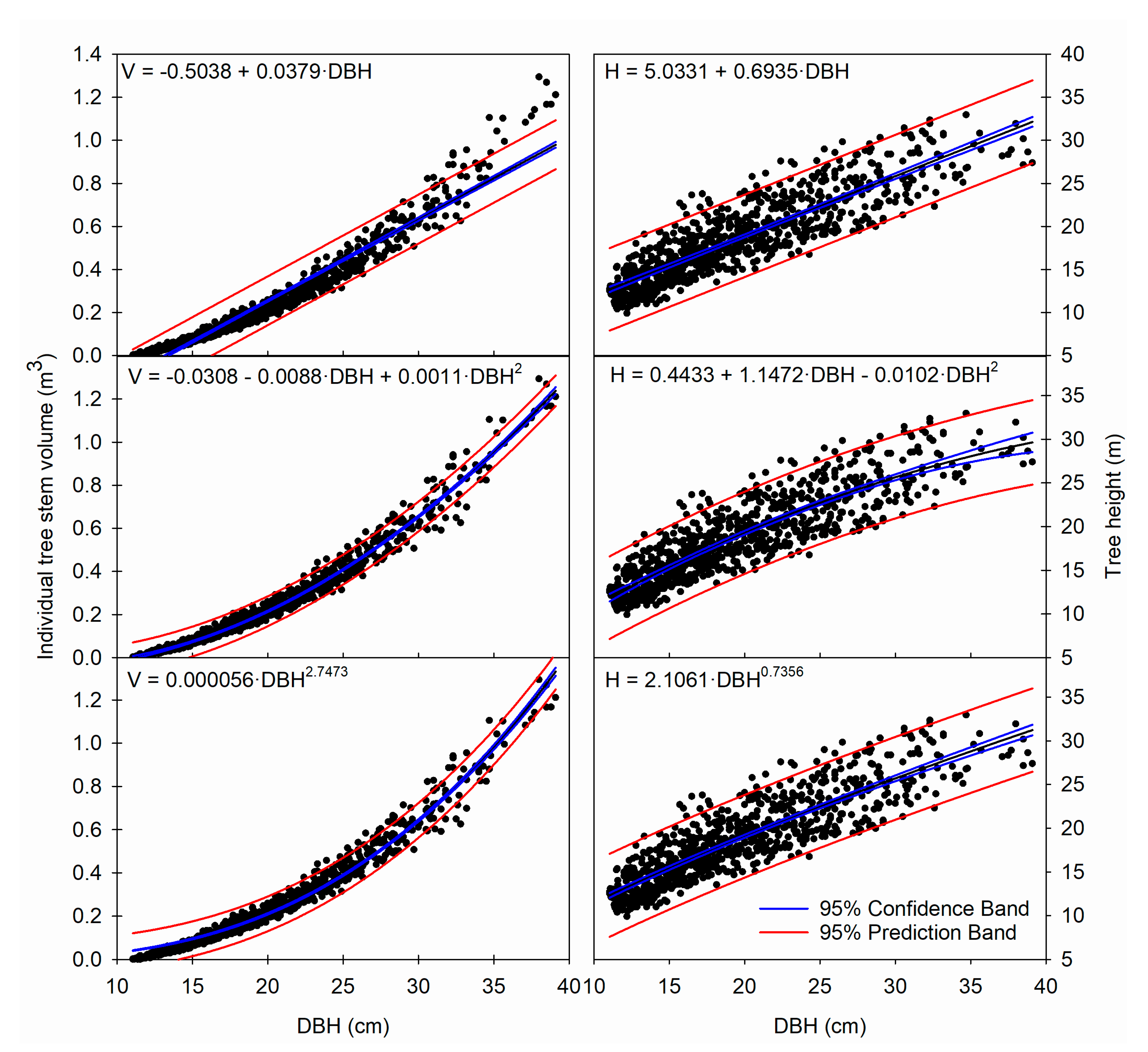
Estimations of stem volume based solely on DBH showed a high model accuracy, as all equations reached adjusted coefficients of determination (R²_adj) above 0.94, with all parameters being significant (

Table 4. Parameter values, their significance and standard errors for the equations tested. For volume, linear: V(m³) = Y₀ + A·DBH(m); Quadratic: V(m³) = Y₀ + A + B·DBH(m); Power: V(m³) = A·DBH(m)^B. For height, linear: H(m) = Y₀ + A·DBH(m); Quadratic: H(m) = Y₀ + A + B·DBH(m); Power: H(m) = A·DBH(m)^B. Significancy levels *: significant with p > 0.05; **: significant with p < 0.001 at α = 0.05.

Equation	Y0	A	B	R2adj	SEestimate
Volume
Linear	−0.5038 ** ± 0.0071	0.0379 ** ± 0.0003	-	0.9418	0.0577
Quadratic	−0.0308 * ± 0.0013	−0.0088 ** ± 0.0013	0.0011 ** ± 2.9·10−5	0.9782	0.0353
Power	-	0.000056 ** ± 3.7·10−6	2.7473 ** ± 0.0196	0.9709	0.0408
Height
Linear	5.0331 ** ± 0.2994	0.6935 ** ± 0.0143	-	0.7521	2.4357
Quadratic	0.4433 ± 0.9425	1.1472 ** ± 0.0896	−0.0102 ** ± 0.0020	0.7600	2.3966
Power	-	2.1061 ** ± 0.0982	0.7356** ± 0.0151	0.7575	2.4092

). Not surprisingly, the linear model for volume underestimated values for the smallest and largest trees, whereas the power equation overestimated volume for the largest trees. However, the quadratic model showed balanced predictions along the whole data range (Figure 1). On the other hand, the higher data dispersion for tree height values caused that height models reached lower coefficient of determination than volume models (0.75–0.76, Table 4), although all the models’ parameters were significant (except slope in the quadratic equation). There were not visible differences among equations in model behavior, with the three height models failing to estimate heights of the tallest trees in the DBH 15–25 cm range.

As described before, the validation dataset was created by randomly selecting 10–11 trees in each plot. The attributes for those trees were very similar to the whole data set, maintaining the same differences among plots observed in the full dataset (

Table 5. Summary data for the trees in the validation dataset in August 2019 (mean ± standard deviation). Different letters indicate differences among plots Tukey’s HSD at α = 0.05.

Variable	Plot 1	Plot 2	Plot 3	All Plots
Number of trees	10	10	11	31
DBH (cm)	24.93 ± 7.543a	24.30 ± 3.41a	24.37 ± 3.61a	24.83 ± 4.98
Height (m)	25.25 ± 5.54a	21.58 ± 4.02b	20.26 ± 2.16c	22.01 ± 4.29
Slenderness index (m/m)	104.1 ± 16.9a	92.3 ± 7.5b	87.6 ± 8.2c	93.4 ± 13.3
Tree volume (m3)	0.519 ± 0.405a	0.454 ± 0.145a	0.337 ± 0.139b	0.395 ± 0.257
Tree basal area (m2)	0.053 ± 0.031a	0.053 ± 0.011a	0.044 ± 0.013a	0.046 ± 0.020

), which indicated such validation dataset was a good representation of the trees in these sites.

Model performance for volume showed the smallest average bias for the power equation, but the smallest mean absolute difference and RMSE for the quadratic model. The quadratic equation also showed low U and high ME coefficients, being closely followed by the power model, and at some distance the linear equation. RMSE values were quite small, ranging from 0.034 m³ for the quadratic model to 0.056 m³ for the linear model. For the quadratic and power models, Freese’s critical errors e* were 0.062 and 0.065 m³ for the exigent user, and 0.042 y 0.045 m³ for the relaxed user, respectively. Hence, only model users demanding accuracy levels lower than those errors would reject those models (

Table 6. Models’ performance indicators when comparing recorded and simulated trees in the validation dataset. MAD: Mean Absolute Difference; RMSE: root mean square error; U: Theil’s coefficient; ME: modelling efficiency; e* = Freese’s critical error.

Equation	Average Bias	MAD	RMSE	U	ME	e* α = 0.05	e* α = 0.20
Volume
Linear	0.032	0.041	0.056	0.287	0.918	0.101	0.069
Quadratic	0.067	0.026	0.034	0.176	0.969	0.062	0.042
Power	0.011	0.029	0.037	0.188	0.965	0.066	0.045
Height
Linear	−0.003	2.058	2.547	0.555	0.691	4.610	3.134
Quadratic	0.002	2.046	2.531	0.552	0.695	4.582	3.115
Power	0.000	2.053	2.534	0.553	0.694	4.588	3.119

).

The three height equations showed small average bias (less than one centimeter), indicating that the models could capture the average of the observed dispersion acceptably well. However, the mean absolute differences (about 2.05 m for all models), and RMSE values (about 2.53 m for all models) were notably higher and quite similar among models, indicating that the models were less able to capture the variability around the mean of the observed tree heights. Similarly, Theil’s coefficients were moderate (0.552–0.555), as well as modelling efficiencies (0.691–0.694). Freese’s critical values also indicated low predictive power of the height models, as even the less demanding user would reject the equivalence of the predicted and observed values if the expected accuracy were less than 3.12–3.13 m, a noticeable value (Table 6).

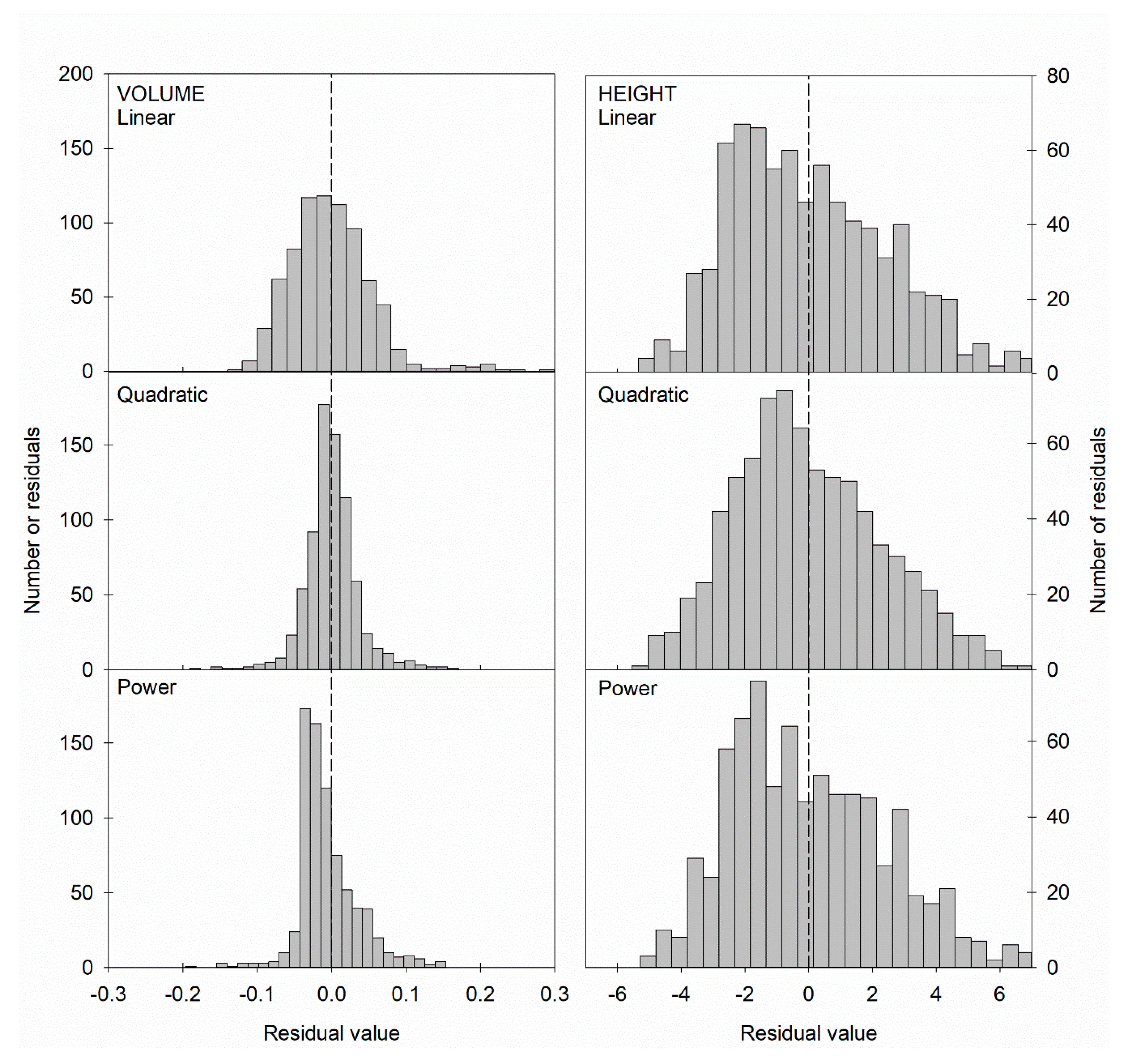
Differences between volume and height models were also evident when comparing residual distributions. Although in all cases distributions significantly departed from normality, the volume models showed more normal-like distributions, particularly the quadratic model. For height, all models showed residuals clearly different from normal distributions, although the quadratic model was also the one with a more balanced residual distribution (Figure 2).

Not surprisingly, the differences among model performances were reflected in the estimated values for some standard DBHs (

Table 7. Tree volume and height for predicted intervals at 95% probability for selected DBH values.

DBH (cm)	Volume (m3 stem−1)			Height (m)
	Linear	Quadratic	Power	Linear	Quadratic	Power
10	0.000–0.009	0.000–0.062	0.000–0.113	7.10–16.84	6.09–15.68	6.64–16.27
15	0.000–0.180	0.014–0.155	0.014–0.177	10.56–20.31	10.55–20.13	10.62–20.26
20	0.139–0.370	0.163–0.304	0.129–0.293	14.03–23.77	14.49–24.09	14.26–23.90
25	0.328–0.559	0.366–0.507	0.308–0.471	17.50–27.24	17.93–27.52	17.66–27.30
30	0.518–0.749	0.625–0.766	0.561–0.725	20.97–30.71	20.86–30.44	20.89–30.53
35	0.707–0.938	0.938–1.079	0.900–1.064	24.43–34.18	23.27–32.86	23–98-33.61
40	0.897–1.128	1.307–1.448	1.335–1.499	27.90–37.64	25.18–34.76	26.95–36.58

). All models showed better accuracy for large than for small trees. Estimated volumes for the typical harvest sizes (DBH > 30 cm and higher) showed relatively narrow prediction intervals, particularly for the quadratic model. However, prediction intervals for tree height were quite large, reaching almost a 10 m difference between the lowest and the highest interval limits (Table 7).

4. Discussion

4.1. Simplified Volume and Height Equations

Relationships among tree attributes are determined by tree architecture and growing conditions. As seen in this work, some poplar trees planted in the Órbigo River basin can reach commercial (harvesting) sizes (DBH > 30 cm) 13 years after planting. However, the stands as a whole had average DBH of 24.78 cm at plantation age 13 years, and assuming annual growth rates between the average and the maximum observed for the new following years (1.66 to 2.39 cm⁻¹ year⁻¹), trees may need 15.2–16.1 years to reach commercial size (DBH > 30 cm). Hence, our results also show that the typical rotation length used by plantation owners in the region (which is about 15 years) is well fitted with the timing of maximum annual volume increment. Those relatively long rotation times for a fast-growing species such as hybrid poplar are typical for this region. Even so, the Duero River basin is considered as a region of good potential productivity for poplars [13]. However, our results also indicate soil fertility as the most likely factor determining differences in growth rates among plots. Although the climate, geology and parent soil material are virtually the same, Plots 1 and 2 showed higher productivity than Plot 3. Plot 2 was established on a farmland used for decades as pasture before plantation establishment. Plot 1was also used for long time as a pasture before planting a poplar stand 15 years prior to current plantation establishment. Consequently, these plots have kept organic matter levels much higher than Plot 3, which was used in intensive farming since reparcelling in the late 1980s (which involved soil movement and mixing), until plantation establishment in 2005. All these processes have resulted in the loss of soil organic matter and its associated fertility. In spite of this, the three plots reached an annual productivity of about 12 m³ ha⁻¹ year⁻¹, considered good for this region [13], and reached the typical productivity range recorded in poplar plantations in the Duero River basin [14].

Although soil fertility has been shown to be the main influential factor on growth rates at these sites, other plot-specific factors may have affected the shape and growth rates of the monitored trees. Trees in Plot 1 had the highest slenderness index, whereas trees in Plot 3 had the lowest. Such differences are likely due to the effect of neighboring farmlands. Plot 3 is surrounded by annual crops in all sides that produced no shading interference with poplar saplings as they grew. Plot 2 was bordered by poplar plantations in the southern side at planting time that provided shade during sapling development. Plot 1 (the most fertile of the three plots) was surrounded by other poplar plantations in its east, south and west sides at planting time. As poplar is a shade-intolerant pioneer genus, it is sensitive to light competition [37]. Hence, shade from neighboring stands had likely forced height growth in those saplings planted under partial shade [38,39,40]. However, surrounding plantations may not have been always a negative influence, as they could have also offered saplings shelter from wind, hence favoring height growth [41].

Another indication of light limitation could be the longer time needed in Plots 1 and 2 to reach maximum annual growths in diameter and height, compared to Plot 3 (about 2 to 5 years longer, Table 2). Such delay could also be related to more intense effects of pruning in reducing self-shading in those plots with other neighboring poplar plantations [42]. Finally, although the three plots were irrigated the same number of times at similar dates during summers, Plot 1 was the closest one to a small permanent stream, while Plot 3 was the furthest. This fact could have forced trees in Plot 3 to invest more in root development. However, trees in Plot 1 could reach water closer to the soil surface, therefore releasing biomass to invest in height growth, as it has been proven in other plantations [43,44,45]. All this plot-level variability in growing conditions has caused a high variability in tree height among trees of the same age. Such variability has been translated in height models with wide confidence intervals for estimated heights.

Because of the intense height growth, combined with pruning [46], some trees became quite slender [47]. This fact, combined with the lengthy plantation time and dense plantation spacing, can make trees quite susceptible to windthrow, as indicated by slender indexes above 100 [48,49]. Trees broken or fallen by wind are economic losses that may cancel the benefit of extending rotation times to reach larger diameters. Therefore, although some authors suggest 35 cm DBH as the optimum for harvesting [7], and suggest harvesting rotations up to 18 years depending on site quality [50], waiting the expected 17–18 years needed at these plots to reach such diameters may be risky. Hence, we suggest that after passing 14–15 years since plantation, owners in the Órbigo River basin must evaluate the potential benefit of letting trees grow another year (which could bring about 1.7–2.3 cm potential DBH increase) versus potential losses by wind. On the other hand, the high slenderness values reached in these plots could also be used as an argument to suggest forest owners to avoid planting poplar next to other plantations already established, because such neighboring plantations could force new saplings to grow very slender to avoid shading [51,52,53]. Later, when neighboring plantations are harvested, such slender saplings are suddenly exposed to wind, increasing windthrow risk.

The diameter and height ranges observed in the monitored plots are inside the reported range for poplar plantations in the Duero River Basin [1,28,29], demonstrating the representability of the selected plots as typical poplar plantations in the floodplains of the Órbigo River basin. However, in spite of the observed differences in soil fertility and tree height, we must highlight the lack of differences among plots in DBH. This fact corroborates the assumption that poplars have some capacity to maintain high productivity rates even when growing in former agricultural soils with low productivity [54].

Keeping in mind the initial hypothesis and the purpose of this research, such lack of differences in DBH among plots is vital for forest owners, as diameter is the only variable that they can easily monitor, and hence the only stand attribute used to make management decisions. Therefore, from the plantation owner’s point of view, the three plots were equivalent, even though the significant differences in height and volume reported here. Following this argument, we developed equations to estimate tree volume from DBH, combining data from trees belonging to all the three plots. We are aware that, from an academic point of view, such combination of plots and ages can be criticized given the significant differences found among plots. However, here again we must remind readers that our objective was developing simple equations usable by non-professionals in a large range of site productivities, rather than creating the most accurate equations to estimate tree volume. In addition, we used data from the age range 5 to 14 years-old and not only from the final harvesting time, to better represent tree development in the models. Although trees change their allometry as they age [55], the obtained volume models have shown to be robust. Hence, we can accept our initial hypothesis, as the quadratic volume equation has shown a high level of accuracy and acceptable model performance. Second in performance was the power equation, while the linear equation displayed important biases for the smallest and largest trees in the observed range. However, we have to recognize that our secondary objective was not met, as the developed equations for tree height have shown only moderate predictive capacity. In spite of that, our results also show that trees have the capacity to maintain similar annual volume growths by changing their allometry, even when height growths are significantly different among plots, as shown by the much robust models for volume than for height.

For the forest owners to make management decisions, it is crucial to know timber market prices at the time of harvest. However, even more important is to know how much standing volume is present in their plantation. Although there are already several volume equations for poplar plantations in Spain [14,15,16,17], they have always been created to reach maximum accuracy by following statistical procedures available only to specialists, as they all use two or more tree attributes (e.g., diameter and height). In fact, our results for the height models also show the difficulty of estimating tree heights as it is a variable very dependent on plot-level environmental variables. This fact only reinforces the need for developing generalized volume equations that use DBH as the only predictor. In addition, most of the plantation owners are seniors already retired or that will reach retirement age during the current rotation, and with little capacity to follow advanced technical procedures by lack of equipment or training. As tree height is difficult to be precisely measured without specific (and usually expensive) equipment such hypsometers, two-variable equations are out of reach in practical terms for most forest owners. Other regular approaches that do not need calculations such as growth and yield tables for plantations densities and by given DBH and height values are also available for poplar [56]. However, tree height is not easy to measure (or even estimate, as our results show) with enough accuracy to be used in those tables with some reliability.

In the Órbigo River basin, most current plantation owners were born and raised in 20th Century post-Civil War Spain, with little opportunity to study beyond primary school, if they were even able to complete it [19,20]. Hence, applying any technical leaflet, report or guideline that displays traditional volume equations is likely out of their reach. Only in the last years, these owners are starting to have access to smartphones, but they still mistrust (or just do not understand) apps or other software that could implement such complex equations.

The accuracy of the equations developed here should be more than enough to provide volume estimations adequate for forest owners to make decisions on harvesting schedules, as indicated by the reduced values of Freese’s critical errors. This is especially useful, as estimated volumes are a better information on timber stocks than just tree diameters. In addition, the equations provided here are simple enough (particularly the linear and quadratic models) that can be written in any regular calculator integrated in a smartphone. Such simplicity allows the forest owner to measure their trees with a regular measuring tape, introduce the circumference in the smartphone’s calculator and just converting it into diameter and then into tree volume. Such simple calculations will provide non-trained forest owners with the capacity to initiate negotiations with timber companies on the time and cost of plantation harvesting from a much stronger position than if volume estimation is left into the hands of the same company that has to buy and harvest the trees.

4.2. Limitations of the Simplification Approach

The approach used here to provide simplified and generalized volume equations has been developed with practicality and usefulness for the intended final user in mind. This means that a sacrifice has been done in terms of statistical or biological rigor. However, it has been argued that cross-validation (which has generated acceptable values for our volume models) is a better approach for model evaluation than residual distributions [57]. In addition, it could been argued that more accurate volume estimations could be reached by using traditional destructive sampling in the target trees, rather than our approach of using an ensemble of already published volume equations. However, using destructive sampling to increase volume estimation accuracy would have limited the application of the resulting models only to the experimental plots. On the other hand, both methods for volume estimation (destructive sampling or ensemble of equations) are conceptually similar, as both assume than an irregular object such as a tree stem has the same volume of a regular solid defined by a mathematical equation. Hence, using an ensemble of models (volume equations in this case) has been shown to be a valid method to encompass uncertainty due to both sampling and model selection [58,59] when estimating growth poplar plantations. In addition, our approach could also be considered inside the current trend that proposes model simplification as a way to increase model usefulness [60], as in essence is a process in which one predictor (DBH) is used to substitute results obtained by several predictor (DBH, height, etc.). In the end, we should not forget that models are neither right nor wrong, but useful (or not) for the task they were designed, Hence, complex models should be used when simple ones cannot do the work [61,62].

As for the biological representativeness of the proposed equations, both the linear and the quadratic equations could be considered as not realistic enough. In the first case, a linear equation assumes constant growth rates independently of tree size, which is obviously not the case. Bigger trees have more access to light, nutrients and water and more photosynthetic capacity, and therefore grow faster (in the absence of other limiting factors) than smaller trees [63,64]. On the other hand, a quadratic model may be more realistic as volume or height growth would accelerate faster than diameter increases due to the squared term. However, as quadratic equations by definition depict parabolas, it may be the case that the estimated height or volume reaches a minimum for intermediate diameters while increasing for small DBHs. To avoid this issue, the quadratic equations were created and defined only for DBH ≥ 10 cm. In any case, we have to remind again that our objective was to define simple equations that would capture as much observed variability as possible, not to create biologically realistic models.

Regardless of our results, we must point out again that the equations shown here do not pretend to substitute those previously developed for poplar by other researchers for this or other regions, such as the dynamic model by [65]. As those equations incorporate more predictors related to tree shape, management schemes or environmental variables, they are indeed better suited for applications that require more accurate estimation of volume, biomass or carbon stocks in poplar forests, and whose expected user base is composed by technicians or forest specialists. Hence, we caution against using the volume equations showed here for objectives other than the stated: a rapid on-the-fly estimation of standing volume in poplar plantations in the Órbigo River basin by non-trained plantation owners.

5. Conclusions

Our work has demonstrated that simplified volume equations can be developed for hybrid poplar plantations in northwestern Spain. In an increasingly urbanized world with wood and paper products demand on the rise, aging rural owners are turning into hybrid poplar plantations that require minimal maintenance as a way to keep getting income from their farmlands. Our equations provide a simple but acceptably accurate tool to empower these rural owners when estimating standing volume by themselves. Our results also demonstrate the viability of an approach that could be used for any species for which several volume equations are available.

References

- Rueda Fernández, J.; García Caballero, J.L. Parcela de Experimentación de Clones de Chopos LE-3 Gradefes; Junta de Castilla y León: Valladolid, Spain, 2013. [Google Scholar]
- Freer-Smith, P.; Muys, B.; Bozzano, M.; Drössler, L.; Farrelly, N.; Jactel, H.; Korhonen, J.; Minotta, G.; Nijnik, M.; Orazio, C. Plantation forests in Europe: Challenges and opportunities. Sci. Policy 2019, 9. [Google Scholar] [CrossRef]
- Christersson, L. Silvicultura de rotación corta: Un complemento de la silvicultura “convencional”. Unasylva 2006, 57, 223. [Google Scholar]
- Vadell, E.; De-Miguel, S.; Pemán, J. Large-scale reforestation and afforestation policy in Spain: A historical review of its underlying ecological, socioeconomic and political dynamics. Land Use Policy 2016, 55, 37–48. [Google Scholar] [CrossRef]
- Martín-García, J.; Barbaro, L.; Diez, J.J.; Jactel, H. Contribution of poplar plantations to bird conservation in riparian landscapes. Silva Fennica. 2013, 47, 4. [Google Scholar] [CrossRef] [Green Version]
- Díaz, L.; Romero, C. Caracterización económica de las choperas en Castilla y León: Rentabilidad y turnos óptimos; Libro de actas del I Simposio del Chopo: Zamora, Spain, 2001; pp. 489–500. [Google Scholar]
- Fernández Manso, A.; Hernanz Arroyo, G. El Chopo (Populus sp.): Manual de Gestión Forestal Sostenible; Junta de Castilla y León: Valladolid, Spain, 2004. [Google Scholar]
- Ambrosio Torrijos, Y.; Picos Martín, J.; Valero Gutiérrez del Olmo, E. Small non industrial forest owners cooperation examples in Galicia (NW Spain). In Proceedings of the FAO Workshop on Forest Operations Improvements in Farm Forest, Logarska Dolina, Slovenia, 9–14 September 2003. [Google Scholar]
- Dominguez, G.; Shannon, M. A wish, a fear and a complaint: Understanding the (dis)engagement of forest owners in forest management. Eur. J. For. Res. 2011, 130, 435–450. [Google Scholar] [CrossRef]
- Wiersum, K.F.; Elands, B.H.M.; Hoogstra, M.A. Small-scale forest ownership across Europe: Characteristics and future potential. Small Scale For. Econ. Manag. Policy 2005, 4, 1–9. [Google Scholar] [CrossRef]
- Rodriguez-Vicente, V.; Marey-Pérez, M.F. Characterization of nonindustrial private forest owners and teir influence on forest management aims and practices in Northern Spain. Small Scale For. 2009, 8, 479–513. [Google Scholar] [CrossRef]
- Vainio, A.; Paloniemi, R. Forest owners and power: A Foucauldian study on Finnish forest policy. Forest Policy Econ. 2012, 21, 118–125. [Google Scholar] [CrossRef]
- Emil Fraga, E.; Fidalgo, L.; Álvarez Rodríguez, E.; Rodriguez Soalleiro, R.; Oliveira, N.; Sixto, H. Crecimiento a medio turno de plantaciones madereras del clon RASPAJE en suelo ácido en Galicia. In Proceedings of the II Simposio del Chopo; Sociedad Pública de Infraestructuras y Medio Ambiente de Castilla y León: Valladolid, Spain, 2018; pp. 63–72. [Google Scholar]
- Bravo, F.; Grau, J.M.; González Antoñanzas, F. Análisis de modelos de producción para Populus x euroamericana en la cuenca del Duero. For. Syst. 1996, 5, 77–95. [Google Scholar]
- Rodríguez, F.; Molina, C. Análisis de modelos de perfil del fuste y estudio de la cilindricidad para tres clones de chopo (Populus x euramericana) en Navarra. For. Syst. 2003, 12, 73–85. [Google Scholar]
- Barrio-Anta, M.; Sixto Blanco, H.; Cañellas Rey de Viñas, I.; González Antoñanzas, F. Sistema de cubicación con clasificación de productos para plantaciones de Populus x euramericana (Dode) Guinier cv. ‘I-214’ en la meseta norte y centro de España. For. Syst. 2007, 16, 65–75. [Google Scholar]
- Rodríguez, F.; Pemán, J.; Aunços, A. A reduced growth model based on stand basal area. A case for hybrid poplar plantations in northeast Spain. For. Ecol. Manag. 2010, 259, 2093–2102. [Google Scholar] [CrossRef]
- Hjelm, B. Stem taper equations for poplars growing on farmland in Sweden. J. For. Res. 2013, 24, 15–22. [Google Scholar] [CrossRef]
- Instituto Nacional de Estadística–INE. Encuesta Sobre la Estructura de las Explotaciones Agrícolas. Available online: https://www.ine.es/dyngs/INEbase/es/operacion.htm?c=Estadistica_C&cid=1254736176854&menu=ultiDatos&idp=1254735727106 (accessed on 3 January 2021).
- Carreras, A.; Tafunell, X. Estadísticas Históricas de España: Siglos XIX-XX, 2nd ed.; Fundación BBVA: Bilbao, Spain, 2005. [Google Scholar]
- Marziliano, P.A.; Russo, D.; Altieri, V.; Macrì, G.; Lombardi, F. Optimizing the sample size to estimate growth in I-214 poplar plantations at definitive tree density for bioenergetic production. Agron. Res. 2018, 16, 821–837. [Google Scholar]
- Köppen, W.; Geiger, R. Das Geographische System der Klimate; Borntraeger: Berlin, Germany, 1936. [Google Scholar]
- Agencia Española de Meteorología–AEMET. 2020. Regionalización AR4-IPCC. Gráficos de evolución. Regionalización estadística análogos. Castilla y León. Accedido el 3 de febrero de 2020. Available online: http://www.aemet.es/es/serviciosclimaticos/cambio_climat/result_graficos?w=0&opc1=cle&opc2=P&opc3=Anual&opc4=0&opc6=1 (accessed on 10 December 2020).
- Gaussen, H.; Bagnouls, F. Saison Seche et Indice Xerotermique; Université de Toulouse, Faculté des Sciences: Toulouse, Francia, 1953. [Google Scholar]
- World Atlas of Desertification; Cherlet, M.; Hutchinson, C.; Reynolds, J.; Hill, J.; Sommer, S.; von Maltitz, G. (Eds.) Publication Office of the European Union: Luxembourg, 2018. [Google Scholar]
- Instituto Tecnológico Agrario de Castilla y León–ITACYL. Visor de Datos de Suelo. Available online: suelos.itacyl.es/visor_datos (accessed on 3 January 2021).
- Blanco, R. Estimación de Tasas de Crecimiento y Producción de Plantaciones de Chopo (Populus x Euroamericana) en la Ribera Media del Duero. Master’s Thesis, Public University of Navarre, Pamplona, Spain, 2020. [Google Scholar]
- Rueda, J.; García Caballero, J.R. Parcelas de Experimentación de Clones de Chopos LE-4 La Milla del Río; Consejería de Fomento y Medio Ambiente, Junta de Castilla y León: Valladolid, Spain, 2018. [Google Scholar]
- Rueda, J.; García Caballero, J.L.; López Negredo, L.; Gómez Cáceres, C. Parcela de Experimentación de Clones de Chopos LE-1 Valencia de Don Juan; Consejería de Fomento y Medio Ambiente, Junta de Castilla y León: Valladolid, Spain, 2006. [Google Scholar]
- Quinn, G.P.; Keough, M.J. Experimental Design and Data Analysis for Biologists; Cambridge University Press: Cambridge, UK, 2002. [Google Scholar]
- Theil, H. Applied Econometric Forecasting; North-Holland: Amsterdam, The Netherdlands, 1966. [Google Scholar]
- Vanclay, J.; Skovsgaard, J.P. Evaluating forest growth models. Ecol. Model. 1997, 98, 1–12. [Google Scholar] [CrossRef] [Green Version]
- Freese, F. Testing accuracy. For. Sci. 1960, 6, 139–145. [Google Scholar]
- Reynolds, M.R. Estimating the error in model predictions. For. Sci. 1984, 30, 454–469. [Google Scholar]
- Blanco, J.A.; González, E. Exploring the sustainability of current management prescriptions for Pinus caribaea plantations in Cuba: A modelling approach. J. Trop. For. Sci. 2010, 22, 139–154. [Google Scholar]
- Blanco, J.A.; Seely, B.; Welham, C.; Kimmins, J.P.; Seebacher, T.M. Testing the performance of FORECAST, a forest ecosystem model, against 29 years of field data in a Pseudotsuga menziesii plantation. Can. J. For. Res. 2007, 37, 1808–1820. [Google Scholar] [CrossRef]
- Welham, C.; Van Rees, K.C.J.; Seely, B.; Kimmins, J.P. Projected long-term productivity in Saskatchewan hybrid poplar plantations: Weed competition and fertilizer effects. Can. J. For. Res. 2007, 37, 356–370. [Google Scholar] [CrossRef]
- Benomar, L.; DesRochers, A.; Larocque, G.R. The effects of spacing on growth, morphology and biomass production and allocation in two hybrid poplar clones growing in the boreal region of Canada. Trees 2012, 26, 939–949. [Google Scholar] [CrossRef]
- Oliver, C.D.; Larson, B.C. Forest Stand Dynamics: Update Edition; John Wiley and Sons: New York, NY, USA, 1996. [Google Scholar]
- Rodríguez Pleguezuelo, C.R.; Durán Zuazo, V.H.; Bielders, C.; Jiménez Bocanegra, J.A.; PereaTorres, F.; Francia Martínez, J.R. Bioenergy farming using woody crops: A review. Agron. Sustain. Dev. 2015, 35, 95–119. [Google Scholar] [CrossRef] [Green Version]
- Gardiner, B.; Berry, P.; Moulia, B. Review: Wind impacts on plant growth, mechanics and damage. Plant Sci. 2016, 245, 94–118. [Google Scholar] [CrossRef] [PubMed]
- Rauscher, H.M.; Isebrands, J.G.; Host, G.E.; Dickson, R.E.; Dickmann, D.I.; Crow, T.R.; Michael, D.A. ECOPHYS: An ecophysiological growth process model for juvenile poplar. Tree Physiol. 1990, 7, 255–281. [Google Scholar] [CrossRef]
- Asadi, F.; Alimohamadi, A. Assessing the performance of Populus caspica and Populus alba cuttings under different irrigation intervals. Agric. For. 2019, 65, 39–51. [Google Scholar] [CrossRef]
- Bagheri, R.; Ghasemi, R.; Calagari, M.; Merrikh, F. Effect of Different Irrigation Interval on Superior Poplar Clones Yield; Research Institute of Forest and Rangeland—RIFR; FAO: Tehran, Iran, 2005. [Google Scholar]
- Lorenc-Plucinska, G.; Walentynowicz, M.; Lwandowski, A. Poplar growth and wood production on a grassland irrigated for decades with potato starch wastewater. Agrofor. Syst. 2017, 91, 307–324. [Google Scholar] [CrossRef] [Green Version]
- Petty, J.A.; Swain, C. Factors influencing stem breakage in high winds. Forestry 1985, 58, 75–84. [Google Scholar] [CrossRef]
- Orzel, S. A comparative analysis of slenderness of the main tree species of the Niepolomice forest. Electron. J. Pol. Agric. Univ. 2007, 10, 13. [Google Scholar]
- Wang, Y.; Titus, S.J.; LeMay, V. Relationships between tree slenderness coefficients and tree or stand characteristics for major species in boreal mixedwood forests. Can. J. For. Res. 1998, 28, 1171–1183. [Google Scholar] [CrossRef]
- Navratil, S. Silvicultural systems for managing deciduous and mixedwood stands with white spruce understory. In Silvicultural of Temperate and Boreal Broadleaf-Conifer Mixture; Comeau, P.G., Thomas, K.D., Eds.; B.C. Ministry of Forests: Victoria, BC, Canada, 1996; pp. 35–46. [Google Scholar]
- Rueda, J.; García Caballero, J.L.; Cuevas, Y.; García-Jiménez, C.; Villar, C. Cultivo de chopos en Castilla y León; Consejería de Fomento y Medio Ambiente, Junta de Castilla y León: Valladolid, Spain, 2019. [Google Scholar]
- DeBell, D.S.; Harrington, C.A. Productivity of Populus in monoclonal and polyclonal blocks at three spacings. Can. J. For. Res. 1997, 27, 978–985. [Google Scholar] [CrossRef]
- Nguyen, T.H. Effects of Thinning on Growth and Development of Second Poplar Generations. Master’s Thesis, Southern Swedish Forest Research Centre, Swedish University of Agricultural Sciences, Alnarp, Sweden, 2018. no. 303. [Google Scholar]
- Feng, J.; Huang, P.; Wan, X. Interactive effects of wind and light on growth and architecture of poplar saplings. Ecol. Res. 2019, 34, 94–105. [Google Scholar] [CrossRef]
- United States Department of Agriculture. USDA. Hybrid Poplar: An Alternative Crop for the Intermountain West; USDA Technical note on Plant Materials no. 37; USDA: Aberdeen, WA, USA, 2001. [Google Scholar]
- Truax, B.; Gagnon, D.; Fortier, J.; Lambert, F. Biomass and volume yield in mature hybrid poplar plantations on temperate abandoned farmland. Forests 2014, 5, 3107–3130. [Google Scholar] [CrossRef] [Green Version]
- Montoya Oliver, J.M. Chopos y Choperas; Mundi Prensa: Madrid, Spain, 1988. [Google Scholar]
- Sileshi, G.W. A critical review of forest biomass estimation models, common mistakes and corrective measures. For. Ecol. Manag. 2014, 329, 237–254. [Google Scholar] [CrossRef]
- Wang, F.; Mladenoff, D.J.; Forrester, J.A.; Blanco, J.A.; Schelle, R.M.; Peckham, S.D.; Keough, C.; Lucash, M.S.; Gower, S.T. Multimodel simulations of forest harvesting effects on long-term productivity and CN cycling in aspen forests. Ecol. Appl. 2014, 24, 1374–1389. [Google Scholar] [CrossRef] [Green Version]
- Lo, Y.H.; Blanco, J.A.; González de Andrés, E.; Imbert, J.B.; Castillo, F.J. CO2 fertilization plays a minor role in long-term carbon accumulation patterns in temperate pine forests in the Pyrenees. Ecol. Model. 2019, 407, 108737. [Google Scholar] [CrossRef]
- Wu, S.; Harris, T.J.; McAuley, K.B. The use of simplified or misspecified models: The linear case. Can. J. Chem. Eng. 2007, 85, 386–398. [Google Scholar] [CrossRef]
- Kimmins, J.P.; Blanco, J.A.; Seely, B.; Welham, C.; Scoullar, K. Complexity in Modeling Forest Ecosystems; How Much is Enough? For. Ecol. Manag. 2008, 256, 1646–1658. [Google Scholar] [CrossRef]
- Blanco, J.A. Modelos ecológicos: Descripción, explicación y predicción. Ecosistemas 2013, 22, 1–5. [Google Scholar] [CrossRef] [Green Version]
- Dietrich, R.; Anand, M. Trees do not always act their age: Size-deterministic tree ring standardization for long-term trend estimation of shade-tolerant trees. Biogeosciences 2019, 16, 4815–4827. [Google Scholar] [CrossRef] [Green Version]
- Blanco, J.A.; Lo, Y.H.; Welham, C.; Larson, B. Productivity of forest ecosystems. In Sustainable Forest Management: From Principles to Practice; Innes, J.I., Tikina, A., Eds.; Earthscan: London, UK, 2017; pp. 72–100. [Google Scholar]
- Barrio-Anta, M.; Sixto-Blanco, H.; Cañellas-Rey de Viñas, I.; Castedo-Dorado, F. Dynamic growth model for I-214 poplar plantations in the northern and central plateaux in Spain. For. Ecol. Manag. 2008, 255, 1167–1178. [Google Scholar] [CrossRef]
Figure 1.
Estimation of tree volume (left panels) and tree height (right panels) under three different equations (showed in each panel) with tree DBH as the only predictor. Dots indicate observed values from the parameterization dataset.
Figure 2.
Distribution of residuals for the three models for each variable with the parameterization dataset (left panels: stem volume; right panels: tree height).