
Monitoring Forest Phenology in a Changing World


Department of Life Sciences, Imperial College London, Silwood Park Campus, Buckhurst Road, Ascot, Berkshire SL5 7PY, UK
*
Author to whom correspondence should be addressed.
Forests 2021, 12(3), 297; https://0-doi-org.brum.beds.ac.uk/10.3390/f12030297
Submission received: 1 February 2021
/
Revised: 1 March 2021
/
Accepted: 2 March 2021
/
Published: 5 March 2021
(This article belongs to the Section Forest Ecology and Management)
Abstract
:Plant phenology is strongly interlinked with ecosystem processes and biodiversity. Like many other aspects of ecosystem functioning, it is affected by habitat and climate change, with both global change drivers altering the timings and frequency of phenological events. As such, there has been an increased focus in recent years to monitor phenology in different biomes. A range of approaches for monitoring phenology have been developed to increase our understanding on its role in ecosystems, ranging from the use of satellites and drones to collection traps, each with their own merits and limitations. Here, we outline the trade-offs between methods (spatial resolution, temporal resolution, cost, data processing), and discuss how their use can be optimised in different environments and for different goals. We also emphasise emerging technologies that will be the focus of monitoring in the years to follow and the challenges of monitoring phenology that still need to be addressed. We conclude that there is a need to integrate studies that incorporate multiple monitoring methods, allowing the strengths of one to compensate for the weaknesses of another, with a view to developing robust methods for upscaling phenological observations from point locations to biome and global scales and reconciling data from varied sources and environments. Such developments are needed if we are to accurately quantify the impacts of a changing world on plant phenology.
1. Introduction
Phenology is the study of the timing of recurrent biological events (or phenophases), the causes of these timings in regard to the biotic and abiotic drivers, and the connection among phases of the same or different species [1]. Here, phenology is defined by both describing observable events and also by describing the links and cascading indirect effects that phenological events can have on an ecosystem [2]. This obvious interrelation of phenology with so many aspects of an ecosystem is why it was hardly considered a scientific discipline until the 1900s [3], despite the recording of phenological events dating back thousands of years [4] (Figure 1). Nevertheless, the connection of phenology with multiple facets of the ecosystem makes monitoring it critical for developing our understanding of ecological processes and for managing resources in the face of climate and habitat change [5,6]. As such, there has been a rapid acceleration in the study of phenology and the associated development of new methods and technologies to aid this endeavour (Figure 1). The past two decades in particular have seen increased effort to build interdisciplinary phenological research frameworks that utilise developments in technology to monitor phenology and its links with ecosystem function across species, space and time [4,6,7].
1.1. The Ubiquitous Importance of Plant Phenology
Most biological organisms follow certain life cycle events, but plant phenology is arguably the most studied. Plant phenology includes processes such as leaf emergence, flowering, fruiting, seeding and leaf senescence, and these processes link strongly to ecosystem function and services (Figure 2; [6,31]). Therefore, change to phenological events may have implications for biogeochemical cycles, including that of carbon [32], and for the population dynamics of species connected at different trophic levels or in competitive and mutualistic interactions [33,34]. Plant phenology can further force temporal shifts in animal phenology [22,35], with the potential for phenological mismatching if the species involved do not respond similarly to environmental changes [35,36].
Leaf emergence (flush) phenology (the presence of new leaves on a tree canopy) is particularly important, as it directly controls processes such as primary productivity, carbon sequestration, nutrient cycling, water storage, and competition and coexistence dynamics (Figure 2; [37,38,39,40,41,42]). For example, when canopy trees flush their leaves it alters the water and light environments for coexisting organisms by intercepting more of the incoming solar radiation and reducing throughfall from precipitation, increasing soil water uptake and consequently reducing soil water and soil water evaporation rates (Figure 2; [38,43]). Indirectly, leaf flush can alter the presence of herbivorous insects and consequently shift the presence of insectivorous birds and mammals (Figure 2). For instance, phenological change of oil-seed crops has resulted in changes in the abundance and type of herbivorous insects present in agricultural landscapes, in turn causing diet shifts in insectivorous birds [44]. There is also a feedback loop to this process: some plant species aim to reduce herbivory by altering their phenological activity to flush before insects emerge, or by synchronising their leaf flushing with other plant species to reduce herbivory pressure [31]. Tropical plants that flush their leaves later in the season can suffer significantly higher damage by insects compared to those that flush early or in synchrony during the peak flushing phase [45]. This is not always the case in temperate regions however, where variation in leaf flush timing involves ecological trade-offs. For example, some Oak species (Quercus spp.) in Eastern Europe flush early in the season to avoid summer droughts but consequently suffer from later spring frost and insect herbivory, whereas other Oak species flush up to six weeks later in the season, avoiding insect herbivory but suffering from summer droughts [46,47].
Flowering and fruiting phenologies are often overlooked, possibly because of the more obvious and critical role played by leaf emergence cycles in many ecosystem processes, however, they also remain key drivers of ecosystem processes [3]. Flowering phenology, for example, can directly impact the diversity of both pollinators and plants (Figure 2). Most of the world’s plants rely on animal pollination for successful reproduction, especially in the tropics where the proportion of animal-pollinated species has been estimated at 94% [51]. Flowering phenology has been demonstrated to positively structure mutualistic plant-flower visitor networks [57], as well as regulate their modularity—a measure of decoupling in densely connected networks [58]. In addition, fruiting and seeding can force ecosystem processes such as fruit hording and seed dispersal, which in turn affects the diversity and distribution of taxa at higher trophic levels (Figure 2). For instance, a change in fruiting phenology has influenced the reproductive performance of endangered chimpanzees in Uganda [59], and the timing of mast seeding events in Borneo has led to increases in insect [60] and nomadic vertebrate populations [55].
At a community level, phenological change can, in theory, have reverberating effects on species distributions [61] and assemblages [2,62], as a result of the fine scale changes in abundance and phenological events [4]. For example, a modelling study outlined how the northern limit of plant species’ ranges in the Northern Hemisphere appears to be dictated by the inability to undergo full fruit maturation [61]. Conversely, the southern limit of plant ranges of the South Hemisphere appears to be dictated by the inability to flower or unfold leaves, owing to a lack of chilling temperatures that are necessary to break bud dormancy [61]. However, to our knowledge the effect of fine scale phenological event change on the community level distribution of higher taxa has not yet been tested.
1.2. Phenology in a Changing World
Habitat Change—Anthropogenic pressures on the environment have caused unprecedented rates of habitat loss, fragmentation, and degradation over the last half-century [63,64,65,66,67,68,69,70]. Forest loss, fragmentation, and the resulting edge effects produce fine-scale variations in light, temperature and humidity, that can in turn induce phenological changes. For example, in Southeastern Brazil there was a higher proportion of reproductive trees along forest edges (59% flowering and 73% fruiting) than inside the forest (47% flowering and 29% fruiting) [71]. Moreover, in Costa Rica, flowering and fruiting events were more common, and occurred 15 to 20 days earlier, in forest disturbed by fragmentation in comparison to undisturbed continuous forest [72], and peak flowering in trees isolated by forest fragmentation increased by double but fruit production from those flowers was halved [73]. Although individual flowers in fragmented forests were less likely to produce a mature fruit, at the scale of individual trees, the change in flowering and fruiting phenology in fragmented forest combined to increase reproductive capacity [74]. Even in agricultural landscapes, land-use intensification is the primary driver of variation in leaf flush onset dates, accounting for 66% of the variation compared to 33% caused by climate change, with an increase in leaf flush onset dates by up to 0.67 days per year caused by land-use intensification [75]. The consequences of altered phenology in human-modified forest habitats reverberate throughout ecosystems, transmitted via plant-animal interactions [76]. For example, in the tropical forests of Borneo, tree plots in logged forest were twice as likely to contain fruits or flowers as in unlogged forest [56]. The resultant increase in resource availability was considered a major factor causing correlated increases in the abundance and functional importance of small mammals within logged forests [56].
Climate Change—Phenological events are especially sensitive indicators of global environmental change because they display strong, thresholded responses to gradual changes in abiotic conditions, such as the leaf emergence or senescence patterns defining growth seasons in temperate forests [77]. Therefore, climate change magnifies the role of phenology in the structure and function of ecological systems [5], where shifts in phenology induced through climatic change can have reverberating effects across trophic levels [78]. There are widespread reports of changes to the life cycles of plants and animals in conjunction with climate variation [35,36,79,80,81]. During the past century, the phenology of 10 bee species from Northeastern North America has advanced by a mean of 10.4 days as a result of climate change altering the phenological timings of flowering plants [35]. In Europe, climatic shifts in the Netherlands have caused an increase in the strength of asynchrony between the phenology of the Winter Moth (Operophtera brumata) and their host plant Oak (Quercus robur) [82], and drier conditions over a 17 year period in Spain resulted in higher asynchrony between pollinator butterfly species and their plants [83]. In North America, 48 passerine species showed increasing phenological asynchrony between their migratory arrival and leaf flush dates (a normal cue for migratory arrival) [84]. Even in aquatic systems such as Argentinian lakes, zooplankton have undergone significant shifts in phenological metrics following temperature increases over the last decade [85].
2. Monitoring Phenology
2.1. Synchrony, Asynchrony and the Challenge for Phenological Monitoring
Habitat and climate change are evidently impacting phenology in ways that generate cascading ecosystem impacts, so there is self-evidently a need to monitor plant phenology effectively if we are to understand and mitigate the ecosystem-level effects of these changes [34,86]. This point is not new: Pereira et al. [87] included remotely sensed land-surface plant phenology as one of the six Essential Biodiversity Variables to monitor global change, and the Intergovernmental Panel on Climate Change (IPCC) defined phenology as “perhaps the simplest process to track changes in the ecology of species in response to climate change” [23]. In light of such high profile calls for improved global monitoring of phenology, there is a timely need for a consensus on the monitoring techniques used to quantify phenological patterns and changes.
In most temperate and boreal biomes, plant phenology is seasonal, with individual plant phenologies often synchronising twice annually (spring and autumn) to create community and landscape level changes [40]. In many tropical regions however, phenological events can vary from complete intraspecific or interspecific synchrony (masting) to extreme asynchrony, and from constant activity to recurrent short pulses [31,88]. Moreover, synchronies in phenological events can be intra-annual or supra-annual such as that of the multi-year cycles induced by El Niño Southern Oscillation events [89]. Together, this creates a mosaic of individual and community level phenological events that vary across space and through time. If we then add changes in spatial scales and other dependencies such as changing environmental conditions, coexistence dynamics, individual tree characteristics, and location that all influence phenology [90,91,92], it rapidly becomes apparent that the simple-sounding task of monitoring phenology masks a challenging problem.
Multiple approaches have emerged over the years to monitor phenology including the use of satellite-based sensors, airborne (plane) mounted sensors, UAV (drone) mounted sensors, fixed digital phenological cameras, collection traps, accelerometers, eddy covariance flux towers, micro-coring and dendrometers, visual assessment, citizen science networks, and genetics (summarised in Table 1; historical introduction of each method outlined in Figure 1). Each method has its own advantages and limitations, often making them more applicable in certain environments and contexts. Here, we examine how each method compares when considering key factors that influence the effectiveness of monitoring phenology: spatial resolution, temporal resolution, cost in terms of equipment, acquisition or labour, and data processing and interpretation requirements. Furthermore, we consider each factor in the context of monitoring phenology in different environments or for different purposes.
2.2. A Brief Description of Phenological Monitoring Methods
The monitoring methods we discuss fit into three broad categories: those that use direct visual assessment, those that use spectral characteristics captured by camera, and those that use a proxy such as biomass or gas flux. Visual assessment is the simplest approach, and consists of walking transects within the forest and visually observing tree canopies for the presence of phenological events. In some areas of the tropics where canopies can be extremely high [93], this is sometimes done with binoculars.
Spectral based assessments can be broadly split into three types that relate to the distance of the sensor from the ground, of which the first is remote sensing by satellites. This form of monitoring is best achieved using surface reflectance products that account for the effect of the atmosphere on the measured radiance by the satellite, including the bi-directional reflectance effects (i.e., the fact that the angle of illumination and observation varies and affects measured radiances). These effects can be modelled with the Bi-Directional Reflectance Distribution Function (BRDF) and used to create nadir BRDF-adjusted reflectance (NBAR) [21]. The NBAR bands are then used to calculate a Vegetation Index (VI), mostly in the form of Enhanced VI (EVI) or Normalised Difference VI (NDVI) [30], which has been shown to correlate with Leaf Area Index (LAI), leaf biomass and percent vegetation cover [21,94]. Besides broadband spectral satellite sensors, multiple other sensors have been applied for phenology assessments, such as active and passive microwave sensors, or sensors capable of assessing fluorescence [95,96,97,98,99]. Second, sensors on board planes or UAVs can be used instead of satellites to capture plant spectral characteristics [100]. Finally, cameras can be placed on observation towers above forest canopies [42,101] or on the ground facing up [102]. Slightly different methods are used to segment or isolate the focal plants or regions of interest (ROI) for analysis, and the spectral resolution of the camera being used will determine the exact analysis being conducted on these last two approaches to collecting spectral data. Many methods extract Red-Green-Blue (RGB) pixel channel data in the form of digital numbers (DNs) for individual plants [103,104]. Further non-linear transformations are then made on these DNs to reduce the effects of scene illumination, the result of which are individual RGB chromatic coordinates (Rcc, Gcc, Bcc) [105]. Some studies also calculate an Excess Green value, to emphasis the influence of phenological change on the green band [24]. These chromatic coordinates and the excess green value are used to track changes in phenology through time as phenophases such as leaf flush or leaf senescence cause variations in these chromatic coordinate values [42,106].
The third category consists of approaches that measure direct or indirect proxies of phenology. Collection traps exist in many forms but generally consist of a net raised above the ground under trees or plants that are being monitored [107]. They work by collecting any fallen material from a focal tree, which is then weighed or counted to estimate the quantity of phenology in the canopy. Collection traps have been used in a range of environments to assess leaf phenology [108,109], fruit and seed phenology [107,110,111,112], and their connections to other aspects of ecosystem function such as carbon fluxes [108]. Accelerometers, dendrometers, and micro-coring approaches monitor phenological activity through the approximation of tree mass or growth at a given time [26,29,46]. Accelerometers and dendrometers attach to trees and record movement and growth which can be used to approximate the presence of a phenological change [26,29]. Leaf emergence and leaf drop alter the aboveground tree mass, resulting in a change that is detectable by the accelerometer or dendrometer [29]. Such measures correlate closely with visual assessment of leaf emergence phenology, but to date have failed to accurately detect leaf loss events [29]. Micro-coring consists of taking samples to measure xylem development which is shown to correlate with leaf flush events [26,46]. Alternatively, eddy covariance flux towers measure CO2 fluxes to calculate gross primary productivity (GPP) [113], which can indicate the phenological start and end of season dates [27,114,115]. Fluxes recorded from eddy covariance towers have also be used to validate satellite-based monitoring of phenology [115].
2.3. Trade-Offs among Phenological Monitoring Techniques
Visual assessment from the ground, sometimes using binoculars, has historically been the most common method for monitoring phenology [79], remains one of the most commonly deployed methods, and is heavily relied upon for the validation of sensor based monitoring [116]. Several long-term research studies have been set up using this method, where a group or individual collects data at a single research site or within a single habitat over an extended period of time [117]. Many of the long term visual assessment studies focus on observing one aspect of phenology such as leaf emergence, flowering or fruiting [112,118], rather than recording all phenological events from a representative sample of plant species [3]. Most studies have also focused on temperate regions [119], with phenology having been monitored for more than 10 years in only 26 sites across tropical America, Africa, and Asia [112]. Visual assessment is time and labour intensive, and of only limited effectiveness in environments where vegetation is dense, terrain is steep and plants exceedingly tall such as that of many tropical forests (Table 1). Arguably, however, the biggest limitation of ground surveys is the subjective bias of observers which can reduce the strength of quantitative conclusions that might be made from visually assessed phenology [116]. Nonetheless, ground surveys remain especially important as a means for validating the data collected from other monitoring methods, and schemes and guidelines do exist to help reduce observer bias [120]. Other methods provide alternatives for visual assessment that monitor phenology both directly and indirectly. The following sections summarise the trade-offs between these methods in relation to the decision factors normally associated with choosing a method (Table 1).
2.3.1. Variation in the Spatial Resolution of Phenological Data
Spatial resolution describes the area that is monitored per unit, where the unit for most sensor-based methods is an individual pixel. For non-sensor-based methods, spatial resolution describes the area covered within an individual observation or by an individual device (e.g., accelerometer or collection trap). Satellite mounted sensors form the backbone of the remote sensing approach envisaged by Pereira et al. [87], but until recently they provided relatively low spatial pixel resolution (0.31 to 1000 m) compared to drones or fixed digital cameras (0.02 m) (Table 1). When monitoring at the landscape level, such as studies monitoring the temperate whole-forest seasonal change, satellites can be highly effective for monitoring phenology as they can cover large areas in a few pixels. For example, the Moderate Resolution Imaging Spectroradiometer (MODIS) on board the NASA Terra satellite possesses seven spectral bands that are specifically designed to monitor landscape changes, including phenology [21].
Studies in temperate regions using satellites like Landsat (30 m resolution) and MODIS (500 m resolution) have been effective in modelling leaf flush and senescence dates [21,40,96,121,122]. A multisite study of temperate and boreal forest phenology using Landsat’s phenology algorithm detected two-thirds of start of season and end of season dates over the 32 years included in the analysis [123]. Furthermore, Zhang et al., [75] successfully used Advanced Very High Resolution Radiometer (AVHRR) and MODIS to observe changes in land surface phenology from 1984–2014 that were caused by land-use change.
In the tropics, by contrast, there is a disparity between the scale of plant phenology—often aseasonal and asynchronous—and that of satellite pixel resolution [25]. As phenological changes often occur at the scale of individual tree crowns, most phenology is undetectable by satellite mounted sensors (although see: [124]), and ground-based or UAV mounted cameras can offer a better alternative [125] (Table 1).
A growing number of studies have used an approach based on fixed digital phenological cameras, in a mix of environments, to monitor phenology at high spatial resolution. Once the effective use of digital webcams to monitor spring green-up (leaf flushing) dates was demonstrated in a deciduous forest in North-Central USA [24], the approach has been extended to a wide set of ecosystems: savanna [126]; deciduous broadleaf forest [24,105,127,128,129]; Evergreen Broadleaf Forest [130]; Evergreen Needleleaf Forest [131,132,133]; and a mix of several habitats [42,101,106,134,135]. Similarly, recent studies have utilised UAV mounted cameras to monitor phenology in a variety of biomes, ranging from polar vegetation [136] to tropical forests [137], with the majority of studies to date focused on temperate regions [125,138,139,140,141,142,143]. For example, Klosterman and Richardson [140] found that in an oak-dominated deciduous forest, the Gcc derived from individual-tree pixels within drone imagery increases in spring following budburst and leaf flush, and decreases in autumn following leaf senescence and loss, with the opposite trend occurring for the Rcc. A similar approach adequately recorded phenological change in a multi-species, deciduous evergreen forest [142], and Berra, Gaulton and Barr [125] consistently detected individual tree level leaf flush dates using chromatic coordinates calculated from drone imagery.
2.3.2. Temporal Resolution and Revisit Frequency
Temporal resolution describes the smallest amount of time between site ‘visits’. As with spatial resolution, in regions where phenology happens at low temporal resolutions, or in synchrony, such as temperate and seasonal biomes, monitoring methods like sensors on-board satellites, planes and helicopters, along with collection traps, can be used effectively to monitor plant phenology, with revisit frequencies as low as a few days [125] (Table 1). For example, Higgins et al., [100] used multispectral cameras on-board a helicopter to track changes in the NDVI values of individual trees and grasses in sub-tropical savannah on a greater than weekly basis, from which they inferred leaf flush timing. Collection traps record phenology at a similar temporal resolution, as can micro-cores. The temporal resolution of both techniques is dependent on the frequency at which samples are collected, which may be daily but is typically longer [26,107].
For regions where asynchronous phenology occurs at high frequency (<1 week), methods that have higher revisit frequencies (daily) may be more beneficial (Table 1). In these regions, continuous high temporal resolution monitoring can feasibly be achieved through the use of devices such as accelerometers, dendrometers, fixed digital cameras or eddy covariance flux towers. Fixed digital cameras can take repeat images at temporal resolutions of less than one day, but are limited by viewing angle (often close to horizontal), meaning they can be dominated by plants closest to the camera [125,129,144]. Eddy covariance flux towers, often used in combination with digital cameras [135], can track the changes in gross primary productivity at very high temporal frequency, commonly 30 min intervals [113]. These three methods—accelerometers, fixed digital cameras and eddy covariance flux towers—have the potential to provide phenological data at very fine temporal resolution, but the first two of these methods often monitor just one or a limited number of plant individuals (Table 1). To get an idea of landscape or community level phenology, multiple devices need to be operated in a network, which can be infeasible in environments with challenging topography. Steep topography and its associated turbulence also presents a challenge for the use of eddy-covariance flux towers [145].
UAV mounted cameras offer a good solution to overcome this limitation as they can be flown at low altitude, close to the canopy, where they can resolve individual-level plant phenology for many, potentially thousands, of individuals [146]. Furthermore, UAV revisit times can be optimised to match the temporal resolution of target species [25] (Table 1). Most consumer level UAVs are lightweight (<2 kg [138]), allowing relatively easy transport to remote locations where they can monitor phenology by flying from accessible areas, provided there are accessible areas within the UAV flight range that can be used as a launching site. UAVs are, however, still limited by maximum survey area (<100 ha for quadcopter or <1000 ha for fixed wing) and by battery life (~20 min per battery) which can impact revisit frequency—realistically no more than daily.
2.3.3. Cost Implications of Competing Methods
In many phenological studies, cost represents a major and critical factor in the choice of method. Costs range over several orders of magnitude depending on the price per unit of monitoring equipment and the price of acquiring data from those units (Table 1). Single time point panchromatic high resolution satellite imagery (50 cm) can cost around US$24 per km2 with a minimum order of 100 km2 (=US$2400) and medium resolution (150 cm) around US$5 per km2 with a minimum order of 500 km2 (=US$2500) [147]. However, free satellite data is also available at high spatial and temporal resolutions, especially if the study area is located in North America or Europe [148], with the National Aeronautics and Space Administration (NASA: ~30 m with ~16 day revisit frequency) and the European Space Agency (ESA: ~10 m with ~5 day revisit frequency) hosting freely available datasets [149,150]. Generally, as the monitoring device decreases in size, so does the cost and the area covered. Placing sensors on-board manned aircraft can also be excessively expensive, ranging from several thousand to hundreds of thousands of dollars [25,125]. Per device, fixed digital phenological cameras provide a near-ground (tower) or ground-based remote sensing alternative to satellites or manned-aircraft for around US$1000 [151] or less, depending on the quality of the digital camera being used [152], but will sometimes incur the additional cost of building a tower to attach the camera to (Table 1). This can be avoided by attaching cameras to trees [153], inexpensive poles or pre-existing towers such as those used for eddy covariance flux [135], but this is not always a guaranteed option when establishing new monitoring locations. Similarly, drones are relatively cheap in comparison to the cost of acquiring satellite imagery or whole networks of digital cameras required to survey a suitable area (<US$2000 per aircraft [154]). Yet, UAVs are still more expensive per unit than collection traps, accelerometers, dendrometers, and visually observing plants from the ground [25,125]. Moreover, losses from crashes are not uncommon. In terms of equipment, the cheapest solutions for monitoring are visual assessment using binoculars, dendrometers, or collection traps. Binoculars can cost as little as US$20 for a suitable focal range to monitor canopy phenology, dendrometers can cost US$2 per unit, and collection traps can cost <US$10 per unit. Despite these methods being cheap per unit, it should be noted they can rapidly become costly when including the labour costs of carrying out monitoring surveys, placing traps in the field and collecting material from those traps (Table 1). This is especially true if you compared the cost per tree surveyed rather than the cost per unit to survey. To monitor a whole landscape, labour costs could end up making visual assessment and traps more expensive than alternative options, such as using satellite data of the region if available at a low price point, or to purchase a single UAV which could survey the same area in a much shorter time.
2.3.4. Data Processing and Interpretation
The processing and interpretation of data can be a major factor in determining the effectiveness of a method for monitoring (Table 1). Visually observed data from binoculars written down on paper require very little processing and interpretation; just the transcription from paper to computer databases for analysis. However, the introduction of cloud-based data collection applications such as EpiCollect [155] remove the need for even this form of processing, allowing mobile phone-based data recording in the field that is automatically stored and backed up online in a data table format. Data collected via traps, accelerometers, dendrometers, and microcores is more time consuming to process as it requires the initial collection of phenological samples or records stored in the traps, followed by the processing of those samples and recording in either paper or digital form. Overall, however, the process, apart from microcore samples, requires little expertise and is straightforward to conduct.
By contrast, eddy covariance and remote sensing data—both satellite and near ground (drones and fixed cameras)—typically requires more data processing and expertise to interpret. Studies on phenology that utilise far or near ground remotely sensed data have slightly different methods for data processing and interpretation (See Section 2.2. for more details), but the general workflow includes turning image features into proxies for phenological change. For example, for fixed cameras and UAV imagery this includes identifying a region of interest in the image (often a tree crown), extracting the red-green-blue pixel values from this region of interest, transforming the values into a spectral feature that may indicate the high presence of a certain colour band, and then comparing the spectral features in a time series to examine if there is a change in a specific colour band which may indicate the presence of phenological change. For example, a leaf flush event is characterized by an increase in greenness within the region of interest.
The remote sensing methods arguably require the skill to code in a programming language such as Python, MATLAB or R, and expertise in coding, photogrammetry and image processing as they mostly produce data in the form of images which require processing to extract quantitative information from their pixel contents. Some applications make these data more easily accessible, such as Google Earth Engine [156], where the remotely sensed satellite data has be pre- collected and processed. Similarly, some software, such as TIMESAT [157], reduce the programming requirements by helping with the analysis of remotely sensed data for the user but does still require pre-processing and a thorough understanding of the data to set parameters.
Determining the optimal metric(s) to use for quantifying phenology often requires pre-existing knowledge of the environment. However, for near-ground remote sensing such as fixed cameras and UAVs, most studies follow the standard set by Richardson et al., [24] and Sonnetag et al., [105] of using chromatic coordinates to suppress influences of scene illumination [105]. Similarly, for satellite-based sensing, most studies use the nadir BRDF-adjusted reflectance (NBAR) bands to calculate different Vegetation Indices which correlate with phenological change [21,30,121,144]. Both methods rely on changing spectral characteristics to indicate a phenological event. Both methods are more quantitative than a visual assessment from the ground and have the potential to pick up more subtle changes in spectral characteristics that may be missed by the eye. However, in new environments this method still requires validation using ground observed data, to ensure the correct phenology is associated with the correct spectral change. Future applications that provide easily accessible remotely sensed data, that require no pre-processing, or require no data manipulation experience represent an important development avenue for the study and monitoring of phenology.
2.4. Multi-Mode Collaboration Networks as a Solution for Ground-Based Monitoring
Ground-based phenology monitoring techniques operate over relatively limited spatial extents and are not suited for addressing large-scale questions around the phenological impacts of global change. Collaboration networks—sometimes using citizen science—can begin to alleviate this issue by increasing the number of sites being monitored, leading to very high “collective resolution”.
Several long-term phenological networks have been set up to collect enormous amounts of phenology data across large spatial scales (USA-NPN [22], NECTAR [158], NEON [159]). For example, the NECTAR database encompasses phenological data for over 5000 plant species with time-series data for over 1500 species [158], and the German National Phenology Network has 474 sites with >50 years of data [160]. The data produced from these studies is valuable because most use status monitoring (e.g., presence or absence of leaves) rather than event-based monitoring (leaf flush), which provides explicit information on presence, absence, and duration of phenophases, as well as enabling integration of the phenology of sessile and mobile organisms [161]. Citizen scientists contribute to phenological data in networks such as the USA-National Phenology Network [22], with the benefit of producing datasets that are much larger—both spatially and temporally—than is feasible from a single research group and for a fraction of the costs [117]. As with all visual assessment monitoring, however, both citizen science and observer-based phenological networks are potentially limited by the subjective bias of observers [116], although collection apps that store photos for future consolidation and validation could help resolve this bias [155].
Networks of phenological cameras provide a quantitative alternative for phenological monitoring networks. One such example is the Phenological Camera (PhenoCam) Network, predominately in North America but continuously expanding, with cameras placed above and within canopy at 440 sites in over 10 different biomes [24,133,151]. Similar large scale studies have also been set up in Europe (EuroPhen [162]), Japan (Phenological Eyes Network (PEN) [163]), and Brazil (e-Phenology Network [42]). Nevertheless, camera-based networks remain costly to implement, particularly if a tower needs to be constructed to mount the camera on and if this construction needs to be in a hard to reach location and/or surrounded by trees and undergrowth. Moreover, camera-based monitoring over multiple biomes with multiple cameras can suffer from the variation between environments in exposure, spectral indices used and sensor specifications so the assurance of standardised data requires multiple post hoc adjustments and editing, all of which can be time consuming [151]. Some networks, like PhenoCam, have begun to address these issues by categorising sites into standardised ‘types’, with Type 1 representing sites with cameras using standardised settings regardless of biome or region of interest [164].
3. Emerging Technological Advancements
3.1. High Resolution Satellite Remote Sensing
Until recently, satellites were considered too coarse in their spatial and temporal resolution for many phenological monitoring requirements—such as monitoring individual tree crown changes in the tropics—but recent years have seen deployments of high spatial and temporal resolution satellites that will put satellite based remote sensing at the forefront of future phenological monitoring once more. Although not an emerging technology, the integration of these high resolution remote sensing satellites into phenological monitoring studies is an emerging process, especially in the tropics. Nevertheless, there are already several recent studies that have shown the use of satellite constellations such as PlanetScope and Sentinel-2 to monitor and map phenology at almost daily intervals and at a spatial resolution of 3 to 10 m, respectively [152,165,166], including a study of phenology in an Amazonian evergreen tropical forest [124]. We envisage that in the coming years we will see the increased use of these satellites, alongside even higher resolution satellites such as GeoEye-1 (0.41 m), WorldView-4 (0.31 m) and Pleiades (0.50 m), in phenological monitoring studies.
High resolution satellites can still limited by the high cost of acquiring their data, the availability of on-the-ground validation data [28], the expertise often required for processing and interpretation. However, the increased deployment and use of satellite constellations will in time reduce the costs [167]. Furthermore, the opportunity for researchers to access freely available data through organisations such as the ESA and NASA will hopefully result in a greater body of trained practitioners that can interpret and analyse the data.
3.2. Molecular Methods for Understanding Phenology
New molecular tools are being developed to monitor phenology and will become integrated within larger scale monitoring frameworks in the coming years [89]. Molecular phenology works through the quantification of gene expression from plant samples using qPCR, microarray and RNA-sequencing methods, creating high-resolution molecular phenology data [168]. For example, flowering phenology can be forecast by examining the regulatory expression dynamics of flowering genes [169]. This allows the immediate detection of ‘invisible’ plant phenological changes, rather than the delayed detection that is gained from monitoring just the end phenology such as the presence of flowers [89,168].
Molecular techniques are expensive and require physical samples to be extracted from individual plants, meaning they are unlikely to be widely applied for basic monitoring of phenology. One approach may be using eDNA or eRNA sampling to collect molecular information on phenology from the soil or air surrounding plants. eDNA sampling has become widespread in ecology, with sample kits becoming relatively inexpensive in recent years [170], and although RNA degrades faster in the environment, eRNA sampling kits are being refined [171]. Therefore, eRNA could be used as a means for larger scale molecular monitoring by sampling population level gene expression related to phenological change.
Where in situ molecular monitoring is not feasible, but collection of plant reproductive material is, provenance trials—the process of taking seeds of species from different areas and planting them together in an experiment—may offer a solution. Provenance trials allow molecular monitoring to take place in controlled, easily accessible environments where they can also help us understand and mitigate the effects of climate change on species whose phenology put them at risk [172]. They can do this by providing experimental information on which genotypes may be able to survive the changing climate and how different phenological forms can arise due to variable responses to climate change [172,173]. In regions where tree species span vast areas of climate, provenance trials have been used to examine the variation in phenological forms [172,173], although to date this approach has largely been restricted to temperate species.
We expect, however, that the strength of molecular methods is their promise to provide much clearer insight into the physiological processes driving phenology, rather than as a direct contribution to directly monitoring phenology. These insights will be central to providing the data needed to develop predictive models examining the abiotic and biotic cues driving phenological events. Such understanding, will, in turn, be needed to allow us to predict the evolutionary responses of phenological patterns as a result of environmental change [89,168]. The higher accuracy and greater responsiveness of molecular phenological data means it can be used to parameterise models with only one or two years of data where more traditional, non-molecular methods may require decades of data [168,169]. The construction of phenological models based on this molecular understanding has potential to then inform other monitoring activities. For example, by building more accurate predictive models, we can better direct expensive, high-resolution satellite remote sensing towards locations that are expected to have change at a particular location and time, saving both money and researcher time.
3.3. Beyond the Visible Light Spectrum
Remote sensing, be it far (satellite), intermediate (drone or plane) or near ground (fixed camera), is not restricted to imaging in the visible spectrum alone (380–740 nm). The use of multispectral (380–2500 nm) and hyperspectral (10–12,500 nm) sensors can capture additional phenological variables related to plant chemistry and health that are reflected in the infrared and ultraviolet spectra [30]. Newly launched satellites such as GOSAT (greenhouse gases observing Satellite), for example, can measure very weak, beyond visible leaf spectral changes such as solar-induced chlorophyll fluorescence (SIF), a by-product of photosynthesis [95,96]. Yang et al., [97] showed the use of a ground-based method to correlate SIF with Gross Primary Productivity (GPP) measures, which can in turn be used to monitor phenology change. Passive microwave sensors (0.01–31 cm) onboard satellites have been used to monitor phenology by calculating vegetation optical depth (VOD), which varies with canopy density and structure and correlates with phenological change [98]. Furthermore, Synthetic Aperture Radar (SAR) (~5.5 cm) onboard the Sentinel-1 has recently been gaining traction as a method for monitoring phenology, having successfully mapped the phenology of crops [99].
As sensors become smaller and more affordable, UAVs are becoming a viable alternatives to satellites and planes when it comes to spectral range [174]. Miniature multispectral, hyperspectral or narrowband cameras attached to UAVs are now being used to capture phenological variables related to plant chemistry and health [174,175,176,177]. For example, Berni et al., [175] used multispectral cameras on-board UAVs to estimate leaf area index, chlorophyll content, leaf water stress, and canopy temperature of crops. Similarly, Zarco-Tejada, González-Dugo and Berni [176] used hyperspectral and thermal imaging cameras on-board UAVs to examine water stress in agricultural crops. To date most of these studies have focused on agricultural crops but, as the cost of sensors decreases, we will likely see them used to assess the phenology of natural habitats.
Techniques that use a wider array of spectra have potential to provide a new avenue for phenological monitoring. They will allow indirect measurement of the chemical quantities within the plants, as opposed to relying on indirect measures of these quantities through plant colour. For example, shifts in Gcc values of individual leaves are an indirect measure of the altered concentrations of chlorophyll in new vs. old leaves [178], so we predict that indirect measurement of leaf chlorophyll will improve the accuracy of leaf phenology data beyond what is achievable through a reliance on leaf colour changes alone. Hyperspectral imagery is beginning to be used for mapping leaf traits and chemistry over large forest areas [95,179] and for automated mapping of species distributions [180], but to date this approach has not been used to monitor phenology. We expect this will be an exciting new direction of research in the future, especially with the recent and upcoming launches of new hyperspectral imaging satellites in the EnMAP, PRISMA, and NASA HyspIRI missions [181,182,183,184].
3.4. Automating the Process of Phenological Monitoring
Autonomous monitoring methods that alleviate the need for human labour are in development and will allow phenology to be monitored in near real-time. Satellites require little user input and satellite imagery has been used a lot for automated detection of events such as fires [185] and volcanic activity [186]. Similar, automated methods for monitoring phenology are becoming available. For example, the Harmonized Landsat Sentinel-2 gridded product, that provides radiometric and geometric corrected, near-daily, 30 m resolution data [148], has the potential to be incorporated into autonomous phenology monitor frameworks [165,187].
Automated analysis of phenological data from smaller devices is also feasible given recent developments allowing fixed devices such as digital phenological cameras to continuously record and send data wirelessly over mobile networks or upload links [188]. Developments in autonomous software for flying UAVs also means they can be flown over vegetative areas with little to no user input [189], and it is only a matter of time before the image data from such flights are fed back for automated analysis. The parallel developments in image processing techniques such as Structure-from-Motion (SfM) [190,191,192] and tree crown detection and delineation algorithms [193,194], allow imagery to be autonomously stitched and ROIs to be determined [195,196,197,198,199]. Similar approaches have been used to autonomously detect and identify species [200,201], but have yet to be applied to imagery collected for the purpose of monitoring phenology.
3.5. LiDAR
Light Detection And Ranging (LiDAR) is beginning to be applied in phenology studies [202], along with its more widespread uses in mapping above ground biomass [203] and forest carbon stocks [204]. LiDAR data can estimate leaf area index (LAI) [205], thus repeated measures could detect phenological events like leaf flush and senescence at the scale of individual tree crowns. This method has potential to provide detailed information about the intensity of phenological events that is unavailable through other methods. For example, LiDAR could potentially be used to quantify the total biomass of new (or old) leaves that have been flushed (or lost) per unit time.
Laser scanning equipment can be placed on-board aircraft [206], UAVs [207,208] or conducted from the ground [202], but the cost of LiDAR equipment (~US$100,000) currently leaves it out of reach for most studies as a method for monitoring. We expect, instead, that it will be most usefully deployed in environments such as tropical forests where phenological events vary in intensity at the scale of individual tree crowns.
4. Monitoring Challenges to Be Addressed
4.1. Expanding the Phenological Monitoring Networks
The next steps for phenological monitoring need to include collaborative, quantitative and technology driven studies that incorporate multiple monitoring methods and focus on long-term monitoring networks across a range of biomes. The majority of the long-term phenological studies have been established in northern hemisphere, temperate biomes [159] and there is a need for these long-term monitoring networks to continue expanding into comparatively understudied systems such as southern hemisphere, ‘aseasonal’ tropical, and arid/semi-arid water-limited environments (however, see [209,210,211,212]).
There are of course challenges in these systems that have prevented the effective long-term monitoring of phenology previously, such as the asynchronous, individual tree crown level patterns in tropical forest phenology. Yet, the emerging technological methods of monitoring can overcome many of these limitations, so integrating these new methods into existing networks should be a priority. There are, however, examples of linking technologies and networks that can act as starting points. For example, the integration of fixed cameras into citizen science networks has already occurred, with the partnership of the PhenoCam network and the USA-NPN [151] and similar set ups in the NEON network [159].
Expanding further into more localities and more data-heavy monitoring methods will produce its own challenges with regard to ‘big data’, cross-platform support, the reconciliation of data from varied sources and environments, and the upscaling of phenological observations. Multi-mode, long term monitoring will require large cloud-based data repositories, along with efficient methods to extract phenological metrics and then archive large data files. Thus, a further step in phenological monitoring will need to include options to integrate, process and store the large cross-platform datasets produced by these networks. Developments in machine learning and high throughput processing power should hopefully offer solutions to this problem.
4.2. Compiling and Reconciling Data across Monitoring Methods
A major challenge with long-term, multi-method, multi-biome monitoring is the need to reconcile data from different sources. Simply compiling these data into a single database represents a significant challenge. To start with, the basic formats of data vary significantly and include everything from classified imagery (e.g., UAV photographs with ROIs categorised into different phenological states) through to gene sequences (molecular monitoring). Space and time represent the obvious axes that will allow data to be indexed in a searchable way, but phenological datasets also come in many different spatiotemporal formats and resolutions. These include temporal snapshots in 1, 2 and 3 spatial dimensions from collection traps, imagery and LiDAR, respectively, through to time series data from accelerometers. An obvious starting point for combining the variable spatiotemporal dimensions of different monitoring methods into the same study is to establish pre-collection criteria on the frequency and spatial arrangement for monitoring, but this will often not be possible if data is collated from different sources. Summarising phenological observations through statistical averaging is the next most obvious step for integrating observations from multiple methods. This would require analysts to specify a common spatial and temporal resolution to apply to all datasets and then either upscale or downscale the resolution of individual datasets to meet this common resolution. This involves a trade-off, however, as the most defensible resolution to aggregate data at is given by the resolution of the coarsest dataset. This means users would lose the ability to examine fine-scale patterns obtained from high resolution methods.
Datasets from alternative methods that overlap in space and time represent both an opportunity and a challenge. Overlapping datasets are needed to validate phenological observations made using competing methods, as is commonly achieved by pairing visual observations with aerial or satellite imagery. There remains, however, an opportunity to expand these validations to remove the need for visual observations through the formation of ‘validation chains’, in which one validated product is used to validate the next. Key to achieving this in a robust manner will be appropriate propagation of error to ensure data uncertainty is accurately represented in the final set of classified observations. Classification accuracy could then be used as a quantitative decision tool for deciding on phenology at given sites where competing methods provide different phenological classifications. Such a process would be aided by setting clear standards for phenological metrics that apply across data sources, and by having database systems designed from the start to record classification accuracy alongside observations.
4.3. Upscaling from Monitoring Sites to Biomes
Translating high resolution spatial data into landscape or biome level phenological metrics is needed to take the step from describing site-specific phenology to understanding the ecological impact of phenology at landscape and biome scales. At the simplest level, upscaling happens via the aggregation of point location observations to generate weighted means of phenological occurrences over larger areas, e.g., an average phenological metric across 1 ha [142,159,213]. Other methods have been proposed such as using Bayesian Hierarchical models that incorporate structure and model the uncertainties in aggregated metrics to predict larger scale phenological trends. For example, modelling a single taxa across multiple sites or multiple taxa at individual sites [214,215]. However, many of the previously proposed methods have been for studies in temperate biomes with relatively low diversity. A more significant challenge lies in upscaling phenological metrics in highly diverse environments such as tropical forest systems. Fully automated hierarchical monitoring systems and the construction of validation chains may help with this. In-person observations or fixed camera imagery can be used to calibrate high spatial resolution/intermediate spatial scale UAV imagery, and in turn this UAV data can be used to calibrate medium or low spatial resolution/large spatial scale satellite imagery. This framework could be adapted to the upscaling of temporal phenological patterns as well. By exploiting hierarchies of temporal monitoring, observations made at high temporal resolution can be used to understand the proportion of events that might be missed by low resolution methods. Together, spatial and temporal upscaling provide a framework to simultaneously exploit the outputs from multiple monitoring methods to provide the information needed to more accurately quantify phenology across space and time.
5. The Future for Forest Phenology Monitoring in a Changing World
The impacts of climate and habitat change on phenology will likely vary across regional-to-continental scales and between biomes [2]. If we are to help mitigate these changes, a greater understanding of the phenological dynamics across biomes and across multiple scale is required. Detecting and quantifying the impacts of change on phenology across regions demands an increase in the spatial scale of phenological monitoring alongside an increase in spatiotemporal resolution. This will become possible through judicious use of the different quantitative methods currently available and currently under development. A key focus should be the increased incorporation of molecular methods and hyperspectral sensors in monitoring frameworks, with the ultimate goal of developing a mechanistic understanding of the phenological process. This ambition will be aided by the simultaneous deployment of multiple monitoring methods, allowing the strengths of one to compensate for the limitations of others, and the continued development of effective approaches to upscaling phenological monitoring from point observations on the ground to biome and global scale maps. This requires an expansion of monitoring approaches already in use [22,159]; however, this is still heavily focused on temperate regions. Not all methods developed in these regions translate to the tropics, where high plant diversity and the asynchronous nature of phenology presents a more difficult challenge that is being addressed, but remains an obvious frontier for further methods development.
Author Contributions
R.E.J.G. led the writing of the manuscript. R.M.E. edited and provided comments on manuscript. All authors have read and agreed to the published version of the manuscript.
Funding
This research was funded by the Natural Environment Research Council Centre for Doctoral Training in Quantitative and Modelling Skills in Ecology and Evolution (QMEE), Grant Number: NE/P012345/1.
Data Availability Statement
No new data were created or analysed in this study. Data sharing is not applicable to this article.
Acknowledgments
The authors would like to thank Terhi Riutta for her valuable comments on a prior draft of the manuscript.
Conflicts of Interest
The authors declare no conflict of interest.
References
- Lieth, H. Phenology and Seasonality Modeling; Springer: Berlin, Germany, 1974; Volume 8. [Google Scholar]
- Richardson, A.D.; Keenan, T.F.; Migliavacca, M.; Ryu, Y.; Sonnentag, O.; Toomey, M. Climate change, phenology, and phenological control of vegetation feedbacks to the climate system. Agric. For. Meteorol. 2013, 169, 156–173. [Google Scholar] [CrossRef]
- Abernethy, K.; Bush, E.R.; Forget, P.M.; Mendoza, I.; Morellato, L.P.C. Current issues in tropical phenology: A synthesis. Biotropica 2018, 50, 477–482. [Google Scholar] [CrossRef] [Green Version]
- Cleland, E.E.; Chuine, I.; Menzel, A.; Mooney, H.A.; Schwartz, M.D. Shifting plant phenology in response to global change. Trends Ecol. Evol. 2007, 22, 357–365. [Google Scholar] [CrossRef]
- Miller-Rushing, A.J.; Weltzin, J. Phenology as a tool to link ecology and sustainable decision making in a dynamic environment. New Phytol. 2009, 184, 743–745. [Google Scholar] [CrossRef] [PubMed]
- Morisette, J.T.; Richardson, A.D.; Knapp, A.K.; Fisher, J.I.; Graham, E.A.; Abatzoglou, J.; Wilson, B.E.; Breshears, D.D.; Henebry, G.M.; Hanes, J.M.; et al. Tracking the rhythm of the seasons in the face of global change: Phenological research in the 21st century. Front. Ecol. Environ. 2009, 7, 253–260. [Google Scholar] [CrossRef] [Green Version]
- Pau, S.; Wolkovich, E.M.; Cook, B.I.; Davies, T.J.; Kraft, N.J.; Bolmgren, K.; Betancourt, J.L.; Cleland, E.E. Predicting phenology by integrating ecology, evolution and climate science. Glob. Chang. Biol. 2011, 17, 3633–3643. [Google Scholar] [CrossRef]
- Sparks, T.H.; Menzel, A. Observed changes in seasons: An overview. Int. J. Climatol. A J. R. Meteorol. Soc. 2002, 22, 1715–1725. [Google Scholar] [CrossRef]
- Demarée, G.R.; Rutishauser, T. Origins of the word “phenology”. Eos Trans. Am. Geophys. Union 2009, 90, 291. [Google Scholar] [CrossRef] [Green Version]
- Clark, J.E. The History of British phenology. Q. J. R. Meteorol. Soc. 1936, 62, 19–24. [Google Scholar] [CrossRef]
- Jeffree, E. Some long-term means from The Phenological Reports (1891–1948) of the Royal Meteorological Society. Q. J. R. Meteorol. Soc. 1960, 86, 95–103. [Google Scholar] [CrossRef]
- Salisbury, E.J. Phenology and habitat with special reference to the phenology of woodlands. Q. J. R. Meteorol. Soc. 1921, 47, 251–260. [Google Scholar] [CrossRef]
- McMillan, C. Nature of the plant community. IV. Phenological variation within five woodland communities under controlled temperatures. Am. J. Bot. 1957, 44, 154–163. [Google Scholar] [CrossRef]
- Newman, J.E.; Beard, J.B. Phenological Observations: The Dependent Variable in Bioclimatic and Agrometeorological Studies. Agron. J. 1962, 54, 399–403. [Google Scholar] [CrossRef]
- Jackson, M.T. Effects of microclimate on spring flowering phenology. Ecology 1966, 47, 407–415. [Google Scholar] [CrossRef]
- Snow, D. A possible selective factor in the evolution of fruiting seasons in tropical forest. Oikos 1965, 15, 274–281. [Google Scholar] [CrossRef]
- McClure, H.E. Flowering, fruiting and animals in the canopy of a tropical rain forest. Malay. For. 1966, 29, 182–203. [Google Scholar]
- Cornforth, I. Leaf-fall in a tropical rain forest. J. Appl. Ecol. 1970, 7, 603–608. [Google Scholar] [CrossRef]
- Terborgh, J. Five New World Primates; Princeton University Press: Princeton, NJ, USA, 1983. [Google Scholar]
- Lloyd, D. A phenological classification of terrestrial vegetation cover using shortwave vegetation index imagery. Int. J. Remote Sens. 1990, 11, 2269–2279. [Google Scholar] [CrossRef]
- Zhang, X.; Friedl, M.A.; Schaaf, C.B.; Strahler, A.H.; Hodges, J.C.; Gao, F.; Reed, B.C.; Huete, A. Monitoring vegetation phenology using MODIS. Remote Sens. Environ. 2003, 84, 471–475. [Google Scholar] [CrossRef]
- Rosemartin, A.H.; Crimmins, T.M.; Enquist, C.A.F.; Gerst, K.L.; Kellermann, J.L.; Posthumus, E.E.; Denny, E.G.; Guertin, P.; Marsh, L.; Weltzin, J.F. Organizing phenological data resources to inform natural resource conservation. Biol. Conserv. 2014, 173, 90–97. [Google Scholar] [CrossRef] [Green Version]
- Rosenzweig, C.; Casassa, G.; Karoly, D.J.; Imeson, A.; Liu, C.; Menzel, A.; Rawlins, S.; Root, T.L.; Seguin, B.; Tryjanowski, P. Assessment of observed changes and responses in natural and managed systems. In Climate Change 2007: Impacts, Adaptation and Vulnerability, Contribution of Working Group II to the Fourth Assessment Report of the Intergovernmental Panel on Climate Change; Parry, M., Canziani, O.F., Palutikof, J., van der Linden, P., Hanson, C., Eds.; Cambridge University Press: Cambridge, UK; New York, NY, USA, 2007; Volume 2007, p. 79. [Google Scholar]
- Richardson, A.D.; Jenkins, J.P.; Braswell, B.H.; Hollinger, D.Y.; Ollinger, S.V.; Smith, M.L. Use of digital webcam images to track spring green-up in a deciduous broadleaf forest. Oecologia 2007, 152, 323–334. [Google Scholar] [CrossRef] [PubMed]
- Anderson, K.; Gaston, K.J. Lightweight unmanned aerial vehicles will revolutionize spatial ecology. Front. Ecol. Environ. 2013, 11, 138–146. [Google Scholar] [CrossRef] [Green Version]
- Michelot, A.; Simard, S.; Rathgeber, C.; Dufrêne, E.; Damesin, C. Comparing the intra-annual wood formation of three European species (Fagus sylvatica, Quercus petraea and Pinus sylvestris) as related to leaf phenology and non-structural carbohydrate dynamics. Tree Physiol. 2012, 32, 1033–1045. [Google Scholar] [CrossRef] [Green Version]
- Gonsamo, A.; Chen, J.M.; Price, D.T.; Kurz, W.A.; Wu, C. Land surface phenology from optical satellite measurement and CO2 eddy covariance technique. J. Geophys. Res. Biogeosci. 2012, 117, G03032. [Google Scholar] [CrossRef]
- Zhang, J.; Hu, J.; Lian, J.; Fan, Z.; Ouyang, X.; Ye, W. Seeing the forest from drones: Testing the potential of lightweight drones as a tool for long-term forest monitoring. Biol. Conserv. 2016, 198, 60–69. [Google Scholar] [CrossRef]
- Gougherty, A.V.; Keller, S.R.; Kruger, A.; Stylinski, C.D.; Elmore, A.J.; Fitzpatrick, M.C. Estimating tree phenology from high frequency tree movement data. Agric. For. Meteorol. 2018, 263, 217–224. [Google Scholar] [CrossRef]
- Xue, J.; Su, B. Significant remote sensing vegetation indices: A review of developments and applications. J. Sens. 2017, 2017, 1353691. [Google Scholar] [CrossRef] [Green Version]
- van Schaik, C.P.; Terborgh, J.W.; Wright, S.J. The phenology of tropical forests: Adaptive significance and consequences for primary consumers. Ann. Rev. Ecol. Syst. 1993, 24, 353–377. [Google Scholar] [CrossRef]
- Richardson, A.D.; Black, T.A.; Ciais, P.; Delbart, N.; Friedl, M.A.; Gobron, N.; Hollinger, D.Y.; Kutsch, W.L.; Longdoz, B.; Luyssaert, S. Influence of spring and autumn phenological transitions on forest ecosystem productivity. Philos. Trans. R. Soc. Lond. B Biol. Sci. 2010, 365, 3227–3246. [Google Scholar] [CrossRef] [Green Version]
- Thébault, E.; Fontaine, C. Stability of ecological communities and the architecture of mutualistic and trophic networks. Science 2010, 329, 853–856. [Google Scholar] [CrossRef]
- Morellato, L.P.C.; Alberton, B.; Alvarado, S.T.; Borges, B.; Buisson, E.; Camargo, M.G.G.; Cancian, L.F.; Carstensen, D.W.; Escobar, D.F.E.; Leite, P.T.P.; et al. Linking plant phenology to conservation biology. Biol. Conserv. 2016, 195, 60–72. [Google Scholar] [CrossRef] [Green Version]
- Bartomeus, I.; Ascher, J.S.; Wagner, D.; Danforth, B.N.; Colla, S.; Kornbluth, S.; Winfree, R. Climate-associated phenological advances in bee pollinators and bee-pollinated plants. Proc. Natl. Acad. Sci. USA 2011, 108, 20645–20649. [Google Scholar] [CrossRef] [PubMed] [Green Version]
- Rafferty, N.E.; CaraDonna, P.J.; Bronstein, J.L. Phenological shifts and the fate of mutualisms. Oikos 2015, 124, 14–21. [Google Scholar] [CrossRef] [Green Version]
- Reich, P.B. Phenology of tropical forests: Patterns, causes, and consequences. Can. J. Bot. 1995, 73, 164–174. [Google Scholar] [CrossRef]
- White, M.; Running, S.W.; Thornton, P.E. The impact of growing-season length variability on carbon assimilation and evapotranspiration over 88 years in the eastern US deciduous forest. Int. J. Biometeorol. 1999, 42, 139–145. [Google Scholar] [CrossRef]
- Baldocchi, D.D.; Black, T.; Curtis, P.; Falge, E.; Fuentes, J.; Granier, A.; Gu, L.; Knohl, A.; Pilegaard, K.; Schmid, H. Predicting the onset of net carbon uptake by deciduous forests with soil temperature and climate data: A synthesis of FLUXNET data. Int. J. Biometeorol. 2005, 49, 377–387. [Google Scholar] [CrossRef]
- Polgar, C.A.; Primack, R.B. Leaf-out phenology of temperate woody plants: From trees to ecosystems. New Phytol. 2011, 191, 926–941. [Google Scholar] [CrossRef]
- Wolkovich, E.M.; Cook, B.I.; Davies, T.J. Progress towards an interdisciplinary science of plant phenology: Building predictions across space, time and species diversity. New Phytol. 2014, 201, 1156–1162. [Google Scholar] [CrossRef] [PubMed] [Green Version]
- Alberton, B.; Torres, R.d.S.; Cancian, L.F.; Borges, B.D.; Almeida, J.; Mariano, G.C.; Santos, J.d.; Morellato, L.P.C. Introducing digital cameras to monitor plant phenology in the tropics: Applications for conservation. Perspect. Ecol. Conserv. 2017, 15, 82–90. [Google Scholar] [CrossRef]
- Tabacchi, E.; Lambs, L.; Guilloy, H.; Planty-Tabacchi, A.M.; Muller, E.; Decamps, H. Impacts of riparian vegetation on hydrological processes. Hydrol. Process. 2000, 14, 2959–2976. [Google Scholar] [CrossRef]
- Orłowski, G.; Karg, J.; Karg, G. Functional invertebrate prey groups reflect dietary responses to phenology and farming activity and pest control services in three sympatric species of aerially foraging insectivorous birds. PLoS ONE 2014, 9, e114906. [Google Scholar] [CrossRef] [PubMed]
- Murali, K.; Sukumar, R. Leaf flushing phenology and herbivory in a tropical dry deciduous forest, southern India. Oecologia 1993, 94, 114–119. [Google Scholar] [CrossRef]
- Puchałka, R.; Koprowski, M.; Gričar, J.; Przybylak, R. Does tree-ring formation follow leaf phenology in Pedunculate oak (Quercus robur L.)? Eur. J. For. Res. 2017, 136, 259–268. [Google Scholar] [CrossRef] [Green Version]
- Wesołowski, T.; Rowiński, P. Late leaf development in pedunculate oak (Quercus robur): An antiherbivore defence? Scand. J. For. Res. 2008, 23, 386–394. [Google Scholar] [CrossRef]
- Coley, P.D.; Barone, J. Herbivory and plant defenses in tropical forests. Ann. Rev. Ecol. Syst. 1996, 27, 305–335. [Google Scholar] [CrossRef]
- Bawa, K.S.; Bullock, S.H.; Perry, D.R.; Coville, R.E.; Grayum, M.H. Reproductive biology of tropical lowland rain forest trees. II. Pollination systems. Am. J. Bot. 1985, 72, 346–356. [Google Scholar] [CrossRef]
- Fontaine, C.; Thébault, E.; Dajoz, I. Are insect pollinators more generalist than insect herbivores? Proc. R. Soc. B Biol. Sci. 2009, 276, 3027–3033. [Google Scholar] [CrossRef] [PubMed] [Green Version]
- Ollerton, J.; Winfree, R.; Tarrant, S. How many flowering plants are pollinated by animals? Oikos 2011, 120, 321–326. [Google Scholar] [CrossRef]
- Fleming, T.H.; Muchhala, N. Nectar-feeding bird and bat niches in two worlds: Pantropical comparisons of vertebrate pollination systems. J. Biogeogr. 2008, 35, 764–780. [Google Scholar] [CrossRef]
- Lambert, F. Fig-eating by birds in a Malaysian lowland rain forest. J. Trop. Ecol. 1989, 5, 401–412. [Google Scholar] [CrossRef]
- Ragusa-Netto, J. Fruiting phenology and consumption by birds in Ficus calyptroceras (Miq.) Miq. (Moraceae). Braz. J. Biol. 2002, 62, 339–346. [Google Scholar] [CrossRef] [PubMed]
- Curran, L.; Leighton, M. Vertebrate responses to spatiotemporal variation in seed production of mast-fruiting Dipterocarpaceae. Ecol. Monogr. 2000, 70, 101–128. [Google Scholar] [CrossRef]
- Ewers, R.M.; Boyle, M.J.; Gleave, R.A.; Plowman, N.S.; Benedick, S.; Bernard, H.; Bishop, T.R.; Bakhtiar, E.Y.; Chey, V.K.; Chung, A.Y.C.; et al. Logging cuts the functional importance of invertebrates in tropical rainforest. Nat. Commun. 2015, 6, 6836. [Google Scholar] [CrossRef] [PubMed]
- Encinas-Viso, F.; Revilla, T.A.; Etienne, R.S. Phenology drives mutualistic network structure and diversity. Ecol. Lett. 2012, 15, 198–208. [Google Scholar] [CrossRef]
- Morente-López, J.; Lara-Romero, C.; Ornosa, C.; Iriondo, J.M. Phenology drives species interactions and modularity in a plant-flower visitor network. Sci. Rep. 2018, 8, 9386. [Google Scholar] [CrossRef]
- Thompson, M.E.; Wrangham, R.W. Diet and reproductive function in wild female chimpanzees (Pan troglodytes schweinfurthii) at Kibale National Park, Uganda. Am. J. Phys. Anthropol. 2008, 135, 171–181. [Google Scholar] [CrossRef]
- Iku, A.; Itioka, T.; Kishimoto-Yamada, K.; Shimizu-kaya, U.; Mohammad, F.B.; Hossman, M.Y.; Bunyok, A.; Rahman, M.Y.A.; Sakai, S.; Meleng, P. Increased seed predation in the second fruiting event during an exceptionally long period of community-level masting in Borneo. Ecol. Res. 2017, 32, 537–545. [Google Scholar] [CrossRef]
- Chuine, I. Why does phenology drive species distribution? Philos. Trans. R. Soc. B Biol. Sci. 2010, 365, 3149–3160. [Google Scholar] [CrossRef] [Green Version]
- Augspurger, C.; Cheeseman, J.; Salk, C. Light gains and physiological capacity of understorey woody plants during phenological avoidance of canopy shade. Funct. Ecol. 2005, 19, 537–546. [Google Scholar] [CrossRef]
- Ramankutty, N.; Foley, J.A. Estimating historical changes in global land cover: Croplands from 1700 to 1992. Glob. Biogeochem. Cycles 1999, 13, 997–1027. [Google Scholar] [CrossRef]
- Goldewijk, K.K. Estimating global land use change over the past 300 years: The HYDE database. Glob. Biogeochem. Cycles 2001, 15, 417–433. [Google Scholar] [CrossRef]
- Gibbs, H.K.; Ruesch, A.S.; Achard, F.; Clayton, M.K.; Holmgren, P.; Ramankutty, N.; Foley, J.A. Tropical forests were the primary sources of new agricultural land in the 1980s and 1990s. Proc. Natl. Acad. Sci. USA 2010, 107, 16732–16737. [Google Scholar] [CrossRef] [Green Version]
- Hansen, M.C.; Potapov, P.V.; Moore, R.; Hancher, M.; Turubanova, S.; Tyukavina, A.; Thau, D.; Stehman, S.; Goetz, S.; Loveland, T. High-resolution global maps of 21st-century forest cover change. Science 2013, 342, 850–853. [Google Scholar] [CrossRef] [PubMed] [Green Version]
- Newbold, T.; Hudson, L.N.; Phillips, H.R.; Hill, S.L.; Contu, S.; Lysenko, I.; Blandon, A.; Butchart, S.H.; Booth, H.L.; Day, J. A global model of the response of tropical and sub-tropical forest biodiversity to anthropogenic pressures. Proc. R. Soc. Lond. B Biol. Sci. 2014, 281, 20141371. [Google Scholar] [CrossRef] [PubMed] [Green Version]
- Newbold, T.; Hudson, L.N.; Hill, S.L.; Contu, S.; Lysenko, I.; Senior, R.A.; Börger, L.; Bennett, D.J.; Choimes, A.; Collen, B. Global effects of land use on local terrestrial biodiversity. Nature 2015, 520, 45–50. [Google Scholar] [CrossRef] [PubMed] [Green Version]
- Watson, J.E.; Jones, K.R.; Fuller, R.A.; Marco, M.D.; Segan, D.B.; Butchart, S.H.; Allan, J.R.; McDonald-Madden, E.; Venter, O. Persistent disparities between recent rates of habitat conversion and protection and implications for future global conservation targets. Conserv. Lett. 2016, 9, 413–421. [Google Scholar] [CrossRef]
- Betts, M.G.; Wolf, C.; Ripple, W.J.; Phalan, B.; Millers, K.A.; Duarte, A.; Butchart, S.H.; Levi, T. Global forest loss disproportionately erodes biodiversity in intact landscapes. Nature 2017, 547, 441. [Google Scholar] [CrossRef]
- D’Eça Neves, F.F.; Morellato, L.P.C. Efeitos de borda na fenologi a de árvores em floresta semidecídua de altitude na Serra do Japi, SP. In Novos Olhares da Serra do Japi, 1st ed.; Vasconcellos Neto, J., Polli, P.R., Eds.; Editora da Unicamp: Campinas, Brazil, 2012. [Google Scholar]
- Herrerías-Diego, Y.; Quesada, M.; Stoner, K.E.; Lobo, J.A. Effects of forest fragmentation on phenological patterns and reproductive success of the tropical dry forest tree Ceiba aesculifolia. Conserv. Biol. 2006, 20, 1111–1120. [Google Scholar] [CrossRef]
- Fuchs, E.J.; Lobo, J.A.; Quesada, M. Effects of forest fragmentation and flowering phenology on the reproductive success and mating patterns of the tropical dry forest tree Pachira quinata. Conserv. Biol. 2003, 17, 149–157. [Google Scholar] [CrossRef] [Green Version]
- Cascante, A.; Quesada, M.; Lobo, J.J.; Fuchs, E.A. Effects of dry tropical forest fragmentation on the reproductive success and genetic structure of the tree Samanea saman. Conserv. Biol. 2002, 16, 137–147. [Google Scholar] [CrossRef]
- Zhang, X.; Liu, L.; Henebry, G.M. Impacts of land cover and land use change on long-term trend of land surface phenology: A case study in agricultural ecosystems. Environ. Res. Lett. 2019, 14, 044020. [Google Scholar] [CrossRef] [Green Version]
- Hagen, M.; Kissling, W.D.; Rasmussen, C.; De Aguiar, M.A.; Brown, L.E.; Carstensen, D.W.; Alves-Dos-Santos, I.; Dupont, Y.L.; Edwards, F.K.; Genini, J. Biodiversity, species interactions and ecological networks in a fragmented world. In Advances in Ecological Research; Elsevier: Amsterdam, The Netherlands, 2012; Volume 46, pp. 89–210. [Google Scholar]
- Peñuelas, J.; Filella, I. Phenology feedbacks on climate change. Science 2009, 324, 887–888. [Google Scholar] [CrossRef] [Green Version]
- Parmesan, C. Influences of species, latitudes and methodologies on estimates of phenological response to global warming. Glob. Chang. Biol. 2007, 13, 1860–1872. [Google Scholar] [CrossRef]
- Schwartz, M.D. Phenology: An Integrative Environmental Science; Kluwer Academic Publishers: Dordrecht, The Netherlands, 2003. [Google Scholar]
- Chen, I.-C.; Hill, J.K.; Ohlemüller, R.; Roy, D.B.; Thomas, C.D. Rapid range shifts of species associated with high levels of climate warming. Science 2011, 333, 1024–1026. [Google Scholar] [CrossRef] [PubMed]
- Lenoir, J.; Svenning, J.C. Climate-related range shifts–a global multidimensional synthesis and new research directions. Ecography 2015, 38, 15–28. [Google Scholar] [CrossRef]
- van Asch, M.; Visser, M.E. Phenology of forest caterpillars and their host trees: The importance of synchrony. Ann. Rev. Entomol. 2007, 52, 37–55. [Google Scholar] [CrossRef]
- Donoso, I.; Stefanescu, C.; Martínez-Abraín, A.; Traveset, A. Phenological asynchrony in plant–butterfly interactions associated with climate: A community-wide perspective. Oikos 2016, 125, 1434–1444. [Google Scholar] [CrossRef] [Green Version]
- Mayor, S.J.; Guralnick, R.P.; Tingley, M.W.; Otegui, J.; Withey, J.C.; Elmendorf, S.C.; Andrew, M.E.; Leyk, S.; Pearse, I.S.; Schneider, D.C. Increasing phenological asynchrony between spring green-up and arrival of migratory birds. Sci. Rep. 2017, 7, 1–10. [Google Scholar] [CrossRef] [Green Version]
- Diovisalvi, N.; Odriozola, M.; Garcia de Souza, J.; Rojas Molina, F.; Fontanarrosa, M.S.; Escaray, R.; Bustingorry, J.; Sanzano, P.; Grosman, F.; Zagarese, H. Species-specific phenological trends in shallow Pampean lakes’(Argentina) zooplankton driven by contemporary climate change in the Southern Hemisphere. Glob. Chang. Biol. 2018, 24, 5137–5148. [Google Scholar] [CrossRef]
- de Melo, F.P.L.; Dirzo, R.; Tabarelli, M. Biased seed rain in forest edges: Evidence from the Brazilian Atlantic forest. Biol. Conserv. 2006, 132, 50–60. [Google Scholar] [CrossRef]
- Pereira, H.M.; Ferrier, S.; Walters, M.; Geller, G.N.; Jongman, R.; Scholes, R.J.; Bruford, M.W.; Brummitt, N.; Butchart, S.; Cardoso, A. Essential Biodiversity Variables. Science 2013, 339, 277–278. [Google Scholar] [CrossRef] [Green Version]
- Adamescu, G.S.; Plumptre, A.J.; Abernethy, K.A.; Polansky, L.; Bush, E.R.; Chapman, C.A.; Shoo, L.P.; Fayolle, A.; Janmaat, K.R.; Robbins, M.M. Annual cycles are the most common reproductive strategy in African tropical tree communities. Biotropica 2018, 50, 418–430. [Google Scholar] [CrossRef]
- Sakai, S.; Kitajima, K. Tropical phenology: Recent advances and perspectives. Ecol. Res. 2019, 34, 50–54. [Google Scholar] [CrossRef]
- Sakai, S.; Momose, K.; Yumoto, T.; Nagamitsu, T.; Nagamasu, H.; Hamid, A.A.; Nakashizuka, T. Plant reproductive phenology over four years including an episode of general flowering in a lowland dipterocarp forest, Sarawak, Malaysia. Am. J. Bot. 1999, 86, 1414–1436. [Google Scholar] [CrossRef] [Green Version]
- Pau, S.; Wolkovich, E.M.; Cook, B.I.; Nytch, C.J.; Regetz, J.; Zimmerman, J.K.; Wright, S.J. Clouds and temperature drive dynamic changes in tropical flower production. Nat. Clim. Chang. 2013, 3, 838. [Google Scholar] [CrossRef]
- Bush, E.R.; Abernethy, K.A.; Jeffery, K.; Tutin, C.; White, L.; Dimoto, E.; Dikangadissi, J.-T.; Jump, A.S.; Bunnefeld, N.; Freckleton, R. Fourier analysis to detect phenological cycles using long-term tropical field data and simulations. Methods Ecol. Evol. 2017, 8, 530–540. [Google Scholar] [CrossRef]
- Shenkin, A.; Chandler, C.J.; Boyd, D.S.; Jackson, T.; Disney, M.; Majalap, N.; Nilus, R.; Foody, G.; bin Jami, J.; Reynolds, G. The world’s tallest tropical tree in three dimensions. Front. For. Glob. Chang. 2019, 2, 32. [Google Scholar] [CrossRef] [Green Version]
- Baret, F.; Guyot, G. Potentials and limits of vegetation indices for LAI and APAR assessment. Remote Sens. Environ. 1991, 35, 161–173. [Google Scholar] [CrossRef]
- Guanter, L.; Frankenberg, C.; Dudhia, A.; Lewis, P.E.; Gómez-Dans, J.; Kuze, A.; Suto, H.; Grainger, R.G. Retrieval and global assessment of terrestrial chlorophyll fluorescence from GOSAT space measurements. Remote Sens. Environ. 2012, 121, 236–251. [Google Scholar] [CrossRef]
- Tang, J.; Körner, C.; Muraoka, H.; Piao, S.; Shen, M.; Thackeray, S.J.; Yang, X. Emerging opportunities and challenges in phenology: A review. Ecosphere 2016, 7, e01436. [Google Scholar] [CrossRef] [Green Version]
- Yang, X.; Tang, J.; Mustard, J.F.; Lee, J.E.; Rossini, M.; Joiner, J.; Munger, J.W.; Kornfeld, A.; Richardson, A.D. Solar-induced chlorophyll fluorescence that correlates with canopy photosynthesis on diurnal and seasonal scales in a temperate deciduous forest. Geophys. Res. Lett. 2015, 42, 2977–2987. [Google Scholar] [CrossRef]
- Jones, M.O.; Jones, L.A.; Kimball, J.S.; McDonald, K.C. Satellite passive microwave remote sensing for monitoring global land surface phenology. Remote Sens. Environ. 2011, 115, 1102–1114. [Google Scholar] [CrossRef]
- Meroni, M.; d’Andrimont, R.; Vrieling, A.; Fasbender, D.; Lemoine, G.; Rembold, F.; Seguini, L.; Verhegghen, A. Comparing land surface phenology of major European crops as derived from SAR and multispectral data of Sentinel-1 and-2. Remote Sens. Environ. 2021, 253, 112232. [Google Scholar] [CrossRef] [PubMed]
- Higgins, S.I.; Delgado-Cartay, M.D.; February, E.C.; Combrink, H.J. Is there a temporal niche separation in the leaf phenology of savanna trees and grasses? J. Biogeogr. 2011, 38, 2165–2175. [Google Scholar] [CrossRef]
- Brown, L.A.; Dash, J.; Ogutu, B.O.; Richardson, A.D. On the relationship between continuous measures of canopy greenness derived using near-surface remote sensing and satellite-derived vegetation products. Agric. For. Meteorol. 2017, 247, 280–292. [Google Scholar] [CrossRef] [Green Version]
- Ryu, Y.; Verfaillie, J.; Macfarlane, C.; Kobayashi, H.; Sonnentag, O.; Vargas, R.; Ma, S.; Baldocchi, D.D. Continuous observation of tree leaf area index at ecosystem scale using upward-pointing digital cameras. Remote Sens. Environ. 2012, 126, 116–125. [Google Scholar] [CrossRef]
- Gillespie, A.R.; Kahle, A.B.; Walker, R.E. Color enhancement of highly correlated images. II. Channel ratio and “chromaticity” transformation techniques. Remote Sens. Environ. 1987, 22, 343–365. [Google Scholar] [CrossRef]
- Woebbecke, D.M.; Meyer, G.E.; Von Bargen, K.; Mortensen, D. Color indices for weed identification under various soil, residue, and lighting conditions. Trans. ASAE 1995, 38, 259–269. [Google Scholar] [CrossRef]
- Sonnentag, O.; Hufkens, K.; Teshera-Sterne, C.; Young, A.M.; Friedl, M.; Braswell, B.H.; Milliman, T.; O’Keefe, J.; Richardson, A.D. Digital repeat photography for phenological research in forest ecosystems. Agric. For. Meteorol. 2012, 152, 159–177. [Google Scholar] [CrossRef]
- Klosterman, S.; Hufkens, K.; Gray, J.; Melaas, E.; Sonnentag, O.; Lavine, I.; Mitchell, L.; Norman, R.; Friedl, M.; Richardson, A. Evaluating remote sensing of deciduous forest phenology at multiple spatial scales using PhenoCam imagery. Biogeosciences 2014, 11, 4305–4320. [Google Scholar] [CrossRef] [Green Version]
- Chapman, C.A.; Wrangham, R.; Chapman, L.J. Indices of habitat-wide fruit abundance in tropical forest. Biotropica 1994, 26, 160–171. [Google Scholar] [CrossRef]
- Riutta, T.; Malhi, Y.; Kho, L.K.; Marthews, T.R.; Huaraca Huasco, W.; Khoo, M.; Tan, S.; Turner, E.; Reynolds, G.; Both, S. Logging disturbance shifts net primary productivity and its allocation in Bornean tropical forests. Glob. Chang. Biol. 2018, 24, 2913–2928. [Google Scholar] [CrossRef] [PubMed] [Green Version]
- Niiyama, K.; Ripin, A.; Yasuda, M.; Sato, T.; Shari, N.H.Z. Data paper: Long-term litter production in a lowland dipterocarp forest, Peninsular Malaysia from 1992 to 2017. Ecol. Res. 2019, 34, 30. [Google Scholar] [CrossRef]
- Hart, L.; Grieve, G.; Downs, C. Fruiting phenology and implications of fruit availability in the fragmented Ngele Forest Complex, KwaZulu-Natal, South Africa. S. Afr. J. Bot. 2013, 88, 296–305. [Google Scholar] [CrossRef] [Green Version]
- Oshima, C.; Tokumoto, Y.; Nakagawa, M. Biotic and abiotic drivers of dipterocarp seedling survival following mast fruiting in Malaysian Borneo. J. Trop. Ecol. 2015, 31, 129–137. [Google Scholar] [CrossRef]
- Mendoza, I.; Condit, R.S.; Wright, S.J.; Caubère, A.; Châtelet, P.; Hardy, I.; Forget, P.M. Inter-annual variability of fruit timing and quantity at Nouragues (French Guiana): Insights from hierarchical Bayesian analyses. Biotropica 2018, 50, 431–441. [Google Scholar] [CrossRef]
- Bórnez, K.; Richardson, A.D.; Verger, A.; Descals, A.; Peñuelas, J. Evaluation of VEGETATION and PROBA-V Phenology Using PhenoCam and Eddy Covariance Data. Remote Sens. 2020, 12, 3077. [Google Scholar] [CrossRef]
- Luo, Y.; El-Madany, T.S.; Filippa, G.; Ma, X.; Ahrens, B.; Carrara, A.; Gonzalez-Cascon, R.; Cremonese, E.; Galvagno, M.; Hammer, T.W. Using near-infrared-enabled digital repeat photography to track structural and physiological phenology in Mediterranean tree–grass ecosystems. Remote Sens. 2018, 10, 1293. [Google Scholar] [CrossRef] [Green Version]
- Xin, F.; Xiao, X.; Cabral, O.M.; White, P.M.; Guo, H.; Ma, J.; Li, B.; Zhao, B. Understanding the Land Surface Phenology and Gross Primary Production of Sugarcane Plantations by Eddy Flux Measurements, MODIS Images, and Data-Driven Models. Remote Sens. 2020, 12, 2186. [Google Scholar] [CrossRef]
- Bush, E.R.; Bunnefeld, N.; Dimoto, E.; Dikangadissi, J.T.; Jeffery, K.; Tutin, C.; White, L.; Abernethy, K.A. Towards effective monitoring of tropical phenology: Maximizing returns and reducing uncertainty in long-term studies. Biotropica 2018, 50, 455–464. [Google Scholar] [CrossRef]
- Taylor, S.D.; Meiners, J.M.; Riemer, K.; Orr, M.C.; White, E.P. Comparison of large-scale citizen science data and long-term study data for phenology modeling. Ecology 2019, 100, e02568. [Google Scholar] [CrossRef] [Green Version]
- Chapman, C.A.; Valenta, K.; Bonnell, T.R.; Brown, K.A.; Chapman, L.J. Solar radiation and ENSO predict fruiting phenology patterns in a 15-year record from Kibale National Park, Uganda. Biotropica 2018, 50, 384–395. [Google Scholar] [CrossRef]
- Feeley, K.J.; Stroud, J.T.; Perez, T.M. Most ‘global’reviews of species’ responses to climate change are not truly global. Divers. Distrib. 2017, 23, 231–234. [Google Scholar] [CrossRef]
- Haggerty, B.P.; Mazer, S.J. The Phenology Handbook; University of California: Oakland, CA, USA, 2008; p. 41. [Google Scholar]
- Fisher, J.I.; Mustard, J.F. Cross-scalar satellite phenology from ground, Landsat, and MODIS data. Remote Sens. Environ. 2007, 109, 261–273. [Google Scholar] [CrossRef]
- Pennec, A.; Gond, V.; Sabatier, D. Tropical forest phenology in French Guiana from MODIS time series. Remote Sens. Lett. 2010, 2, 337–345. [Google Scholar] [CrossRef]
- Melaas, E.K.; Sulla-Menashe, D.; Gray, J.M.; Black, T.A.; Morin, T.H.; Richardson, A.D.; Friedl, M.A. Multisite analysis of land surface phenology in North American temperate and boreal deciduous forests from Landsat. Remote Sens. Environ. 2016, 186, 452–464. [Google Scholar] [CrossRef]
- Wang, J.; Yang, D.; Detto, M.; Nelson, B.W.; Chen, M.; Guan, K.; Wu, S.; Yan, Z.; Wu, J. Multi-scale integration of satellite remote sensing improves characterization of dry-season green-up in an Amazon tropical evergreen forest. Remote Sens. Environ. 2020, 246, 111865. [Google Scholar] [CrossRef]
- Berra, E.F.; Gaulton, R.; Barr, S. Assessing spring phenology of a temperate woodland: A multiscale comparison of ground, unmanned aerial vehicle and Landsat satellite observations. Remote Sens. Environ. 2019, 223, 229–242. [Google Scholar] [CrossRef]
- Alberton, B.; Almeida, J.; Helm, R.; Torres, R.D.S.; Menzel, A.; Morellato, L.P.C. Using phenological cameras to track the green up in a cerrado savanna and its on-the-ground validation. Ecol. Inform. 2014, 19, 62–70. [Google Scholar] [CrossRef]
- Ahrends, H.E.; Etzold, S.; Kutsch, W.L.; Stöckli, R.; Brügger, R.; Jeanneret, F.; Wanner, H.; Buchmann, N.; Eugster, W. Tree phenology and carbon dioxide fluxes: Use of digital photography for process-based interpretation at the ecosystem scale. Clim. Res. 2009, 39, 261–274. [Google Scholar] [CrossRef] [Green Version]
- Dragoni, D.; Rahman, A.F. Trends in fall phenology across the deciduous forests of the Eastern USA. Agric. For. Meteorol. 2012, 157, 96–105. [Google Scholar] [CrossRef]
- Hufkens, K.; Friedl, M.; Sonnentag, O.; Braswell, B.H.; Milliman, T.; Richardson, A.D. Linking near-surface and satellite remote sensing measurements of deciduous broadleaf forest phenology. Remote Sens. Environ. 2012, 117, 307–321. [Google Scholar] [CrossRef]
- Zhao, J.; Zhang, Y.; Tan, Z.; Song, Q.; Liang, N.; Yu, L.; Zhao, J. Using digital cameras for comparative phenological monitoring in an evergreen broad-leaved forest and a seasonal rain forest. Ecol. Inform. 2012, 10, 65–72. [Google Scholar] [CrossRef]
- Henneken, R.; Dose, V.; Schleip, C.; Menzel, A. Detecting plant seasonality from webcams using Bayesian multiple change point analysis. Agric. For. Meteorol. 2013, 168, 177–185. [Google Scholar] [CrossRef] [Green Version]
- Kurc, S.; Benton, L. Digital image-derived greenness links deep soil moisture to carbon uptake in a creosotebush-dominated shrubland. J. Arid Environ. 2010, 74, 585–594. [Google Scholar] [CrossRef]
- Richardson, A.D.; Braswell, B.H.; Hollinger, D.Y.; Jenkins, J.P.; Ollinger, S.V. Near-surface remote sensing of spatial and temporal variation in canopy phenology. Ecol. Appl. 2009, 19, 1417–1428. [Google Scholar] [CrossRef]
- Ide, R.; Oguma, H. Use of digital cameras for phenological observations. Ecol. Inform. 2010, 5, 339–347. [Google Scholar] [CrossRef]
- Toomey, M.; Friedl, M.A.; Frolking, S.; Hufkens, K.; Klosterman, S.; Sonnentag, O.; Baldocchi, D.D.; Bernacchi, C.J.; Biraud, S.C.; Bohrer, G. Greenness indices from digital cameras predict the timing and seasonal dynamics of canopy-scale photosynthesis. Ecol. Appl. 2015, 25, 99–115. [Google Scholar] [CrossRef] [Green Version]
- Malenovský, Z.; Lucieer, A.; King, D.H.; Turnbull, J.D.; Robinson, S.A. Unmanned aircraft system advances health mapping of fragile polar vegetation. Methods Ecol. Evol. 2017, 8, 1842–1857. [Google Scholar] [CrossRef] [Green Version]
- Park, J.Y.; Muller-Landau, H.C.; Lichstein, J.W.; Rifai, S.W.; Dandois, J.P.; Bohlman, S.A. Quantifying Leaf Phenology of Individual Trees and Species in a Tropical Forest Using Unmanned Aerial Vehicle (UAV) Images. Remote Sens. 2019, 11, 1534. [Google Scholar] [CrossRef] [Green Version]
- Dandois, J.P.; Ellis, E.C. High spatial resolution three-dimensional mapping of vegetation spectral dynamics using computer vision. Remote Sens. Environ. 2013, 136, 259–276. [Google Scholar] [CrossRef] [Green Version]
- Berra, E.F.; Gaulton, R.; Barr, S. Commercial off-the-shelf digital cameras on unmanned aerial vehicles for multitemporal monitoring of vegetation reflectance and NDVI. IEEE Trans. Geosci. Remote Sens. 2017, 55, 4878–4886. [Google Scholar] [CrossRef] [Green Version]
- Klosterman, S.; Richardson, A.D. Observing Spring and Fall Phenology in a Deciduous Forest with Aerial Drone Imagery. Sensors 2017, 17, 2852. [Google Scholar] [CrossRef] [Green Version]
- Burkart, A.; Hecht, V.; Kraska, T.; Rascher, U. Phenological analysis of unmanned aerial vehicle based time series of barley imagery with high temporal resolution. Precis. Agric. 2018, 19, 134–146. [Google Scholar] [CrossRef]
- Klosterman, S.; Melaas, E.; Wang, J.; Martinez, A.; Frederick, S.; O’Keefe, J.; Orwig, D.A.; Wang, Z.; Sun, Q.; Schaaf, C. Fine-scale perspectives on landscape phenology from unmanned aerial vehicle (UAV) photography. Agric. For. Meteorol. 2018, 248, 397–407. [Google Scholar] [CrossRef]
- Neumann, C.; Behling, R.; Schindhelm, A.; Itzerott, S.; Weiss, G.; Wichmann, M.; Müller, J. The colors of heath flowering–quantifying spatial patterns of phenology in Calluna life-cycle phases using high-resolution drone imagery. Remote Sens. Ecol. Conserv. 2019, 6, 35–61. [Google Scholar] [CrossRef] [Green Version]
- Liu, Y.; Hill, M.J.; Zhang, X.; Wang, Z.; Richardson, A.D.; Hufkens, K.; Filippa, G.; Baldocchi, D.D.; Ma, S.; Verfaillie, J. Using data from Landsat, MODIS, VIIRS and PhenoCams to monitor the phenology of California oak/grass savanna and open grassland across spatial scales. Agric. For. Meteorol. 2017, 237, 311–325. [Google Scholar] [CrossRef]
- Baldocchi, D.; Finnigan, J.; Wilson, K.; Falge, E. On measuring net ecosystem carbon exchange over tall vegetation on complex terrain. Bound. Layer Meteorol. 2000, 96, 257–291. [Google Scholar] [CrossRef]
- Getzin, S.; Wiegand, K.; Schöning, I. Assessing biodiversity in forests using very high-resolution images and unmanned aerial vehicles. Methods Ecol. Evol. 2012, 3, 397–404. [Google Scholar] [CrossRef]
- Land Info Worldwide Mapping LLC. Buying Satellite Imagery: Pricing Information for High Resolution Satellite Imagery. Available online: http://www.landinfo.com/satellite-imagery-pricing.html (accessed on 19 October 2019).
- Claverie, M.; Ju, J.; Masek, J.G.; Dungan, J.L.; Vermote, E.F.; Roger, J.-C.; Skakun, S.V.; Justice, C. The Harmonized Landsat and Sentinel-2 surface reflectance data set. Remote Sens. Environ. 2018, 219, 145–161. [Google Scholar] [CrossRef]
- European Space Agency—ESA. Earth Online. Available online: https://earth.esa.int/eogateway/ (accessed on 22 February 2021).
- The National Aeronautics and Space Administration—NASA. Data. Available online: https://nasa.github.io/data-nasa-gov-frontpage/ (accessed on 27 February 2021).
- Richardson, A.D.; Hufkens, K.; Milliman, T.; Aubrecht, D.M.; Chen, M.; Gray, J.M.; Johnston, M.R.; Keenan, T.F.; Klosterman, S.T.; Kosmala, M. Tracking vegetation phenology across diverse North American biomes using PhenoCam imagery. Sci. Data 2018, 5, 180028. [Google Scholar] [CrossRef]
- Cheng, Y.; Vrieling, A.; Fava, F.; Meroni, M.; Marshall, M.; Gachoki, S. Phenology of short vegetation cycles in a Kenyan rangeland from PlanetScope and Sentinel-2. Remote Sens. Environ. 2020, 248, 112004. [Google Scholar] [CrossRef]
- Liu, N.; Garcia, M.; Singh, A.; Clare, J.D.; Stenglein, J.L.; Zuckerberg, B.; Kruger, E.L.; Townsend, P.A. Trail camera networks provide insights into satellite-derived phenology for ecological studies. Int. J. Appl. Earth Obs. Geoinf. 2021, 97, 102291. [Google Scholar] [CrossRef]
- Koh, L.P.; Wich, S.A. Dawn of drone ecology: Low-cost autonomous aerial vehicles for conservation. Trop. Conserv. Sci. 2012, 5, 121–132. [Google Scholar] [CrossRef] [Green Version]
- Aanensen, D.M.; Huntley, D.M.; Feil, E.J.; Spratt, B.G. EpiCollect: Linking smartphones to web applications for epidemiology, ecology and community data collection. PLoS ONE 2009, 4, e6968. [Google Scholar] [CrossRef] [PubMed] [Green Version]
- Gorelick, N.; Hancher, M.; Dixon, M.; Ilyushchenko, S.; Thau, D.; Moore, R. Google Earth Engine: Planetary-scale geospatial analysis for everyone. Remote Sens. Environ. 2017, 202, 18–27. [Google Scholar] [CrossRef]
- Jönsson, P.; Eklundh, L. TIMESAT—A program for analyzing time-series of satellite sensor data. Comput. Geosci. 2004, 30, 833–845. [Google Scholar] [CrossRef] [Green Version]
- Wolkovich, E.M.; Cook, B.I.; Allen, J.M.; Crimmins, T.M.; Betancourt, J.L.; Travers, S.E.; Pau, S.; Regetz, J.; Davies, T.J.; Kraft, N.J. Warming experiments underpredict plant phenological responses to climate change. Nature 2012, 485, 494. [Google Scholar] [CrossRef] [PubMed]
- Elmendorf, S.C.; Jones, K.D.; Cook, B.I.; Diez, J.M.; Enquist, C.A.; Hufft, R.A.; Jones, M.O.; Mazer, S.J.; Miller-Rushing, A.J.; Moore, D.J. The plant phenology monitoring design for the national ecological observatory network. Ecosphere 2016, 7, e01303. [Google Scholar] [CrossRef] [Green Version]
- Kaspar, F.; Zimmermann, K.; Polte-Rudolf, C. An overview of the phenological observation network and the phenological database of Germany’s national meteorological service (Deutscher Wetterdienst). Adv. Sci. Res. 2015, 11, 93–99. [Google Scholar] [CrossRef] [Green Version]
- Denny, E.G.; Gerst, K.L.; Miller-Rushing, A.J.; Tierney, G.L.; Crimmins, T.M.; Enquist, C.A.; Guertin, P.; Rosemartin, A.H.; Schwartz, M.D.; Thomas, K.A. Standardized phenology monitoring methods to track plant and animal activity for science and resource management applications. Int. J. Biometeorol. 2014, 58, 591–601. [Google Scholar] [CrossRef] [PubMed] [Green Version]
- Wingate, L.; Ogée, J.; Cremonese, E.; Filippa, G.; Mizunuma, T.; Migliavacca, M.; Moisy, C.; Wilkinson, M.; Moreaux, C.; Wohlfahrt, G. Interpreting canopy development and physiology using the EUROPhen camera network at flux sites. Biogeosci. Discuss. 2015, 12, 5995–6015. [Google Scholar] [CrossRef] [Green Version]
- Nagai, S.; Akitsu, T.; Saitoh, T.M.; Busey, R.C.; Fukuzawa, K.; Honda, Y.; Ichie, T.; Ide, R.; Ikawa, H.; Iwasaki, A. 8 million phenological and sky images from 29 ecosystems from the Arctic to the tropics: The Phenological Eyes Network. Ecol. Res. 2018, 33, 1091–1092. [Google Scholar] [CrossRef]
- Seyednasrollah, B.; Young, A.M.; Hufkens, K.; Milliman, T.; Friedl, M.A.; Frolking, S.; Richardson, A.D. Tracking vegetation phenology across diverse biomes using Version 2.0 of the PhenoCam Dataset. Sci. Data 2019, 6, 1–11. [Google Scholar]
- Bolton, D.K.; Gray, J.M.; Melaas, E.K.; Moon, M.; Eklundh, L.; Friedl, M.A. Continental-scale land surface phenology from harmonized Landsat 8 and Sentinel-2 imagery. Remote Sens. Environ. 2020, 240, 111685. [Google Scholar] [CrossRef]
- Wu, S.; Wang, J.; Yan, Z.; Song, G.; Chen, Y.; Ma, Q.; Deng, M.; Wu, Y.; Zhao, Y.; Guo, Z. Monitoring tree-crown scale autumn leaf phenology in a temperate forest with an integration of PlanetScope and drone remote sensing observations. ISPRS J. Photogramm. Remote Sens. 2021, 171, 36–48. [Google Scholar] [CrossRef]
- Singh, L.A.; Whittecar, W.R.; DiPrinzio, M.D.; Herman, J.D.; Ferringer, M.P.; Reed, P.M. Low cost satellite constellations for nearly continuous global coverage. Nat. Commun. 2020, 11, 1–7. [Google Scholar] [CrossRef]
- Kudoh, H. Molecular phenology in plants: In natura systems biology for the comprehensive understanding of seasonal responses under natural environments. New Phytol. 2016, 210, 399–412. [Google Scholar] [CrossRef] [Green Version]
- Satake, A.; Kawagoe, T.; Saburi, Y.; Chiba, Y.; Sakurai, G.; Kudoh, H. Forecasting flowering phenology under climate warming by modelling the regulatory dynamics of flowering-time genes. Nat. Commun. 2013, 4, 1–8. [Google Scholar] [CrossRef]
- Ruppert, K.M.; Kline, R.J.; Rahman, M.S. Past, present, and future perspectives of environmental DNA (eDNA) metabarcoding: A systematic review in methods, monitoring, and applications of global eDNA. Glob. Ecol. Conserv. 2019, 17, e00547. [Google Scholar] [CrossRef]
- Adams, C.I.; Knapp, M.; Gemmell, N.J.; Jeunen, G.-J.; Bunce, M.; Lamare, M.D.; Taylor, H.R. Beyond biodiversity: Can environmental DNA (eDNA) cut it as a population genetics tool? Genes 2019, 10, 192. [Google Scholar] [CrossRef] [Green Version]
- Robson, T.M.; Rasztovits, E.; Aphalo, P.J.; Alia, R.; Aranda, I. Flushing phenology and fitness of European beech (Fagus sylvatica L.) provenances from a trial in La Rioja, Spain, segregate according to their climate of origin. Agric. For. Meteorol. 2013, 180, 76–85. [Google Scholar] [CrossRef]
- Guo, X.; Klisz, M.; Puchałka, R.; Silvestro, R.; Faubert, P.; Belien, E.; Huang, J.; Rossi, S. Common-garden experiment reveals clinal trends of bud phenology in black spruce populations from a latitudinal gradient in the boreal forest. J. Ecol. 2021, 1–11. [Google Scholar] [CrossRef]
- Adão, T.; Hruška, J.; Pádua, L.; Bessa, J.; Peres, E.; Morais, R.; Sousa, J. Hyperspectral imaging: A review on UAV-based sensors, data processing and applications for agriculture and forestry. Remote Sens. 2017, 9, 1110. [Google Scholar] [CrossRef] [Green Version]
- Berni, J.A.; Zarco-Tejada, P.J.; Suárez, L.; Fereres, E. Thermal and narrowband multispectral remote sensing for vegetation monitoring from an unmanned aerial vehicle. IEEE Trans. Geosci. Remote Sens. 2009, 47, 722–738. [Google Scholar] [CrossRef] [Green Version]
- Zarco-Tejada, P.J.; González-Dugo, V.; Berni, J.A. Fluorescence, temperature and narrow-band indices acquired from a UAV platform for water stress detection using a micro-hyperspectral imager and a thermal camera. Remote Sens. Environ. 2012, 117, 322–337. [Google Scholar] [CrossRef]
- Yang, X.; Tang, J.; Mustard, J.F. Beyond leaf color: Comparing camera-based phenological metrics with leaf biochemical, biophysical, and spectral properties throughout the growing season of a temperate deciduous forest. J. Geophys. Res. Biogeosci. 2014, 119, 181–191. [Google Scholar] [CrossRef] [Green Version]
- Croft, H.; Chen, J.M.; Luo, X.; Bartlett, P.; Chen, B.; Staebler, R.M. Leaf chlorophyll content as a proxy for leaf photosynthetic capacity. Glob. Chang. Biol. 2017, 23, 3513–3524. [Google Scholar] [CrossRef] [PubMed]
- Asner, G.P.; Martin, R.E. Airborne spectranomics: Mapping canopy chemical and taxonomic diversity in tropical forests. Front. Ecol. Environ. 2009, 7, 269–276. [Google Scholar] [CrossRef] [Green Version]
- Vauhkonen, J.; Hakala, T.; Suomalainen, J.; Kaasalainen, S.; Nevalainen, O.; Vastaranta, M.; Holopainen, M.; Hyyppä, J. Classification of spruce and pine trees using active hyperspectral LiDAR. IEEE Geosci. Remote Sens. Lett. 2013, 10, 1138–1141. [Google Scholar] [CrossRef]
- Amato, U.; Antoniadis, A.; Carfora, M.F.; Colandrea, P.; Cuomo, V.; Franzese, M.; Pignatti, S.; Serio, C. Statistical classification for assessing PRISMA hyperspectral potential for agricultural land use. IEEE J. Sel. Top. Appl. Earth Obs. Remote Sens. 2013, 6, 615–625. [Google Scholar] [CrossRef]
- Guanter, L.; Kaufmann, H.; Segl, K.; Foerster, S.; Rogass, C.; Chabrillat, S.; Kuester, T.; Hollstein, A.; Rossner, G.; Chlebek, C. The EnMAP spaceborne imaging spectroscopy mission for earth observation. Remote Sens. 2015, 7, 8830–8857. [Google Scholar] [CrossRef] [Green Version]
- Lee, C.M.; Cable, M.L.; Hook, S.J.; Green, R.O.; Ustin, S.L.; Mandl, D.J.; Middleton, E.M. An introduction to the NASA Hyperspectral InfraRed Imager (HyspIRI) mission and preparatory activities. Remote Sens. Environ. 2015, 167, 6–19. [Google Scholar] [CrossRef]
- Gamon, J.; Somers, B.; Malenovský, Z.; Middleton, E.; Rascher, U.; Schaepman, M.E. Assessing vegetation function with imaging spectroscopy. Surv. Geophys. 2019, 40, 489–513. [Google Scholar] [CrossRef] [Green Version]
- Justice, C.; Giglio, L.; Korontzi, S.; Owens, J.; Morisette, J.; Roy, D.; Descloitres, J.; Alleaume, S.; Petitcolin, F.; Kaufman, Y. The MODIS fire products. Remote Sens. Environ. 2002, 83, 244–262. [Google Scholar] [CrossRef]
- Pergola, N.; Marchese, F.; Tramutoli, V. Automated detection of thermal features of active volcanoes by means of infrared AVHRR records. Remote Sens. Environ. 2004, 93, 311–327. [Google Scholar] [CrossRef]
- Zhang, X.; Wang, J.; Henebry, G.M.; Gao, F. Development and evaluation of a new algorithm for detecting 30 m land surface phenology from VIIRS and HLS time series. ISPRS J. Photogramm. Remote Sens. 2020, 161, 37–51. [Google Scholar] [CrossRef]
- Sethi, S.S.; Ewers, R.M.; Jones, N.S.; Orme, C.D.L.; Picinali, L. Robust, real-time and autonomous monitoring of ecosystems with an open, low-cost, networked device. Methods Ecol. Evol. 2018, 9, 2383–2387. [Google Scholar] [CrossRef] [Green Version]
- Strecha, C.; Küng, O.; Fua, P. Automatic mapping from ultra-light UAV imagery. In Proceedings of the EuroCOW 2012, Barcelona, Spain, 28–30 June 2016. [Google Scholar]
- Snavely, N.; Seitz, S.M.; Szeliski, R. Modeling the world from internet photo collections. Int. J. Comput. Vis. 2008, 80, 189–210. [Google Scholar] [CrossRef] [Green Version]
- Westoby, M.J.; Brasington, J.; Glasser, N.F.; Hambrey, M.J.; Reynolds, J. ‘Structure-from-Motion’photogrammetry: A low-cost, effective tool for geoscience applications. Geomorphology 2012, 179, 300–314. [Google Scholar] [CrossRef] [Green Version]
- James, M.R.; Robson, S.; d’Oleire-Oltmanns, S.; Niethammer, U. Optimising UAV topographic surveys processed with structure-from-motion: Ground control quality, quantity and bundle adjustment. Geomorphology 2017, 280, 51–66. [Google Scholar] [CrossRef] [Green Version]
- Ke, Y.; Quackenbush, L.J. A review of methods for automatic individual tree-crown detection and delineation from passive remote sensing. Int. J. Remote Sens. 2011, 32, 4725–4747. [Google Scholar] [CrossRef]
- Larsen, M.; Eriksson, M.; Descombes, X.; Perrin, G.; Brandtberg, T.; Gougeon, F.A. Comparison of six individual tree crown detection algorithms evaluated under varying forest conditions. Int. J. Remote Sens. 2011, 32, 5827–5852. [Google Scholar] [CrossRef]
- Park, T.-J.; Lee, J.-Y.; Lee, W.-K.; Kwak, D.-A.; Kwak, H.-B.; Lee, S.-C. Automated individual tree detection and crown delineation using high spatial resolution RGB aerial imagery. Korean J. Remote Sens. 2011, 27, 703–715. [Google Scholar] [CrossRef] [Green Version]
- Colomina, I.; Molina, P. Unmanned aerial systems for photogrammetry and remote sensing: A review. ISPRS J. Photogramm. Remote Sens. 2014, 92, 79–97. [Google Scholar] [CrossRef] [Green Version]
- Näsi, R.; Honkavaara, E.; Lyytikäinen-Saarenmaa, P.; Blomqvist, M.; Litkey, P.; Hakala, T.; Viljanen, N.; Kantola, T.; Tanhuanpää, T.; Holopainen, M. Using UAV-based photogrammetry and hyperspectral imaging for mapping bark beetle damage at tree-level. Remote Sens. 2015, 7, 15467–15493. [Google Scholar] [CrossRef] [Green Version]
- Csillik, O.; Cherbini, J.; Johnson, R.; Lyons, A.; Kelly, M. Identification of Citrus Trees from Unmanned Aerial Vehicle Imagery Using Convolutional Neural Networks. Drones 2018, 2, 39. [Google Scholar] [CrossRef] [Green Version]
- Goldbergs, G.; Maier, S.W.; Levick, S.R.; Edwards, A. Efficiency of Individual Tree Detection Approaches Based on Light-Weight and Low-Cost UAS Imagery in Australian Savannas. Remote Sens. 2018, 10, 161. [Google Scholar] [CrossRef] [Green Version]
- Lisein, J.; Michez, A.; Claessens, H.; Lejeune, P. Discrimination of deciduous tree species from time series of unmanned aerial system imagery. PLoS ONE 2015, 10, e0141006. [Google Scholar] [CrossRef]
- Baena, S.; Moat, J.; Whaley, O.; Boyd, D.S. Identifying species from the air: UAVs and the very high resolution challenge for plant conservation. PLoS ONE 2017, 12, e0188714. [Google Scholar]
- Calders, K.; Schenkels, T.; Bartholomeus, H.; Armston, J.; Verbesselt, J.; Herold, M. Monitoring spring phenology with high temporal resolution terrestrial LiDAR measurements. Agric. For. Meteorol. 2015, 203, 158–168. [Google Scholar] [CrossRef]
- Asner, G.P.; Brodrick, P.G.; Philipson, C.; Vaughn, N.R.; Martin, R.E.; Knapp, D.E.; Heckler, J.; Evans, L.J.; Jucker, T.; Goossens, B. Mapped aboveground carbon stocks to advance forest conservation and recovery in Malaysian Borneo. Biol. Conserv. 2018, 217, 289–310. [Google Scholar] [CrossRef]
- Coomes, D.A.; Dalponte, M.; Jucker, T.; Asner, G.P.; Banin, L.F.; Burslem, D.F.; Lewis, S.L.; Nilus, R.; Phillips, O.L.; Phua, M.-H. Area-based vs tree-centric approaches to mapping forest carbon in Southeast Asian forests from airborne laser scanning data. Remote Sens. Environ. 2017, 194, 77–88. [Google Scholar] [CrossRef] [Green Version]
- Korhonen, L.; Korpela, I.; Heiskanen, J.; Maltamo, M. Airborne discrete-return LIDAR data in the estimation of vertical canopy cover, angular canopy closure and leaf area index. Remote Sens. Environ. 2011, 115, 1065–1080. [Google Scholar] [CrossRef]
- Simonson, W.; Allen, H.; Coomes, D. Effect of Tree Phenology on LiDAR Measurement of Mediterranean Forest Structure. Remote Sens. 2018, 10, 659. [Google Scholar] [CrossRef] [Green Version]
- Lin, Y.; Hyyppa, J.; Jaakkola, A. Mini-UAV-borne LIDAR for fine-scale mapping. IEEE Geosci. Remote Sens. Lett. 2010, 8, 426–430. [Google Scholar] [CrossRef]
- Sankey, T.; Donager, J.; McVay, J.; Sankey, J.B. UAV lidar and hyperspectral fusion for forest monitoring in the southwestern USA. Remote Sens. Environ. 2017, 195, 30–43. [Google Scholar] [CrossRef]
- Gordo, O.; Sanz, J.J. Long-term temporal changes of plant phenology in the Western Mediterranean. Glob. Chang. Biol. 2009, 15, 1930–1948. [Google Scholar] [CrossRef]
- Crimmins, T.M.; Crimmins, M.A.; David Bertelsen, C. Complex responses to climate drivers in onset of spring flowering across a semi-arid elevation gradient. J. Ecol. 2010, 98, 1042–1051. [Google Scholar] [CrossRef]
- de Oliveira, C.C.; Zandavalli, R.B.; de Lima, A.L.A.; Rodal, M.J.N. Functional groups of woody species in semi-arid regions at low latitudes. Austral. Ecol. 2015, 40, 40–49. [Google Scholar] [CrossRef]
- Mazer, S.J.; Gerst, K.L.; Matthews, E.R.; Evenden, A. Species-specific phenological responses to winter temperature and precipitation in a water-limited ecosystem. Ecosphere 2015, 6, 1–27. [Google Scholar] [CrossRef] [Green Version]
- Liang, L.; Schwartz, M.D.; Fei, S. Validating satellite phenology through intensive ground observation and landscape scaling in a mixed seasonal forest. Remote Sens. Environ. 2011, 115, 143–157. [Google Scholar] [CrossRef]
- Diez, J.M.; Ibáñez, I.; Miller-Rushing, A.J.; Mazer, S.J.; Crimmins, T.M.; Crimmins, M.A.; Bertelsen, C.D.; Inouye, D.W. Forecasting phenology: From species variability to community patterns. Ecol. Lett. 2012, 15, 545–553. [Google Scholar] [CrossRef] [Green Version]
- Ibáñez, I.; Primack, R.B.; Miller-Rushing, A.J.; Ellwood, E.; Higuchi, H.; Lee, S.D.; Kobori, H.; Silander, J.A. Forecasting phenology under global warming. Philos. Trans. R. Soc. B Biol. Sci. 2010, 365, 3247–3260. [Google Scholar] [CrossRef]
Figure 1.
Timeline history of monitoring phenology. References for the specific time periods are: pre-1700 [4], 1700s [8], 1853 [9], 1900s [10,11], 1920s [12], 1950s [13], 1960s [14,15], 1965-83 [16,17,18,19], 1900s [20], 2003 [21], 2000s [3,22], 2007 [23,24], 2012 [2,25,26,27], 2016 [28,29], and 2020 [30].

Figure 2.
Ecosystem processes and conditions that drive phenological events. References giving examples for the effect of phenology on ecological processes are: increased interception [38], increased herbivory [48], increased pollination [49,50,51], increased nectar feeding [52], increased soil water uptake [38,39,40,41,42,43], increased fruit feeding [53,54], increased seed hoarding [55], increased seed dispersal [55], increased seed predation [56], decreased soil water uptake [38,39,40,41,42,43], decreased leaf decomposition [56], increased solar radiation [2,38,43], increased rain throughfall [38], and decreased solar radiation [2,38,43].


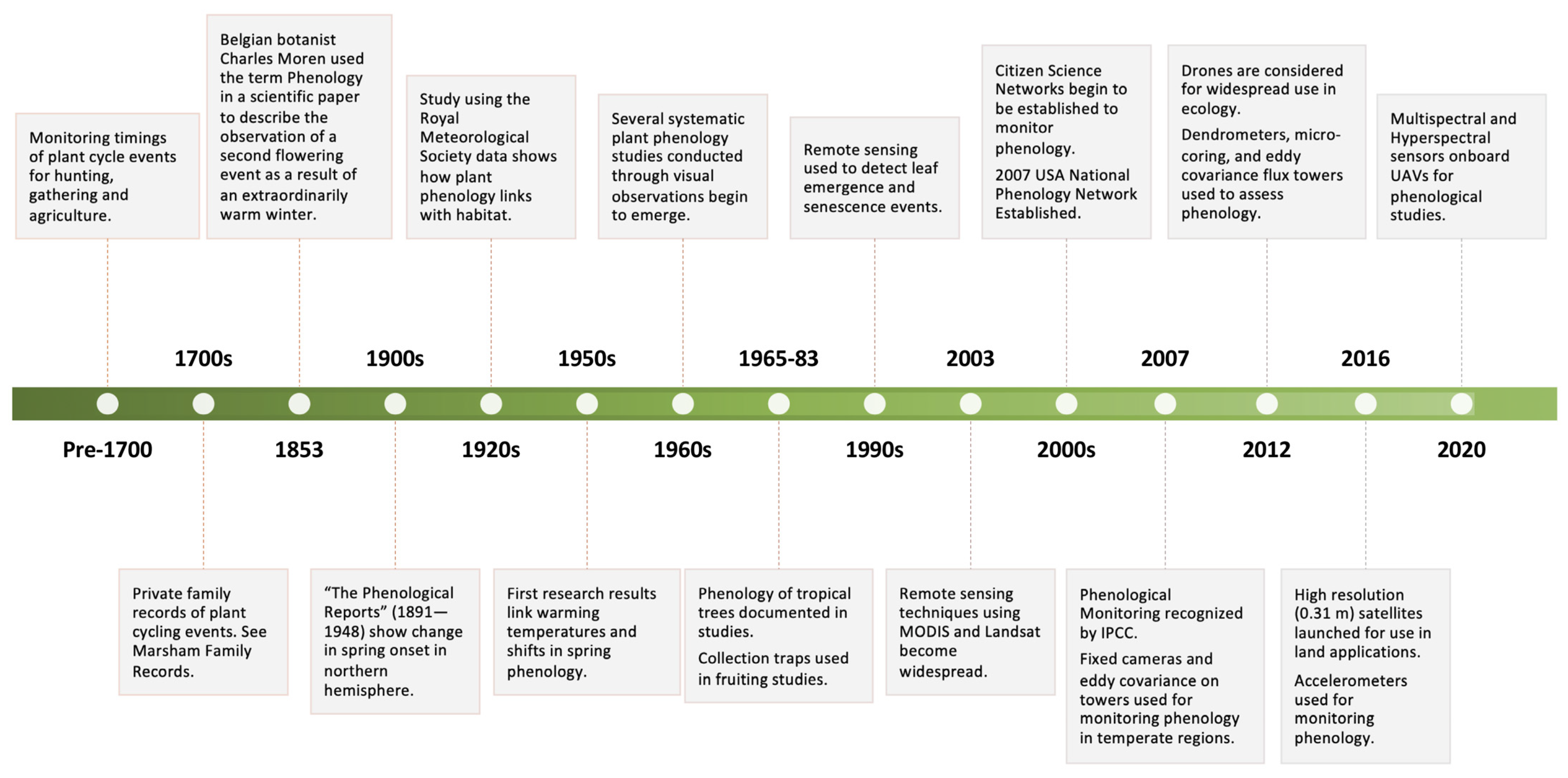
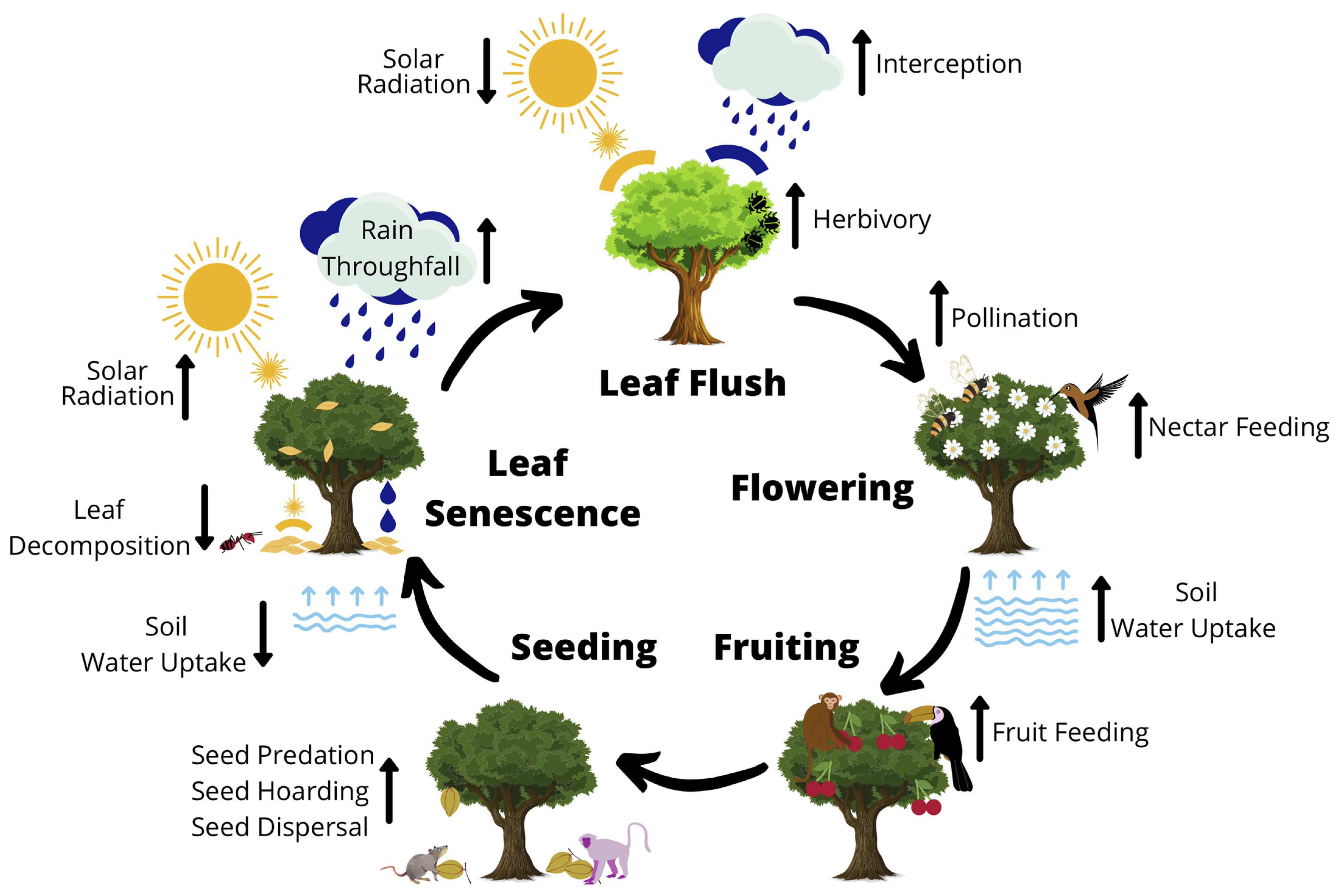
Table 1.
Each phenological monitoring method in a table comparison of key decision factors. From top to bottom: satellites, planes, helicopters, drones (UAVs), fixed digital cameras, human visual observations, accelerometers, eddy covariance flux towers, micro-coring and dendrometers, collection traps. $ = US Dollars. Factors listed as categories can be Low, Medium, or High. High showing the method performs well for the factor and low showing the method performs poorly for the factor. NA indicates where data is not available, or the factor is not applicable for that monitoring method. A semicolon between values indicates a split between equipment cost and set-up cost of the method when deploying it. * indicates the potential cost of constructing a tower if needed.
| Factor | ||||||||||||
|---|---|---|---|---|---|---|---|---|---|---|---|---|
| Monitoring Method | Measurement | Spatial Resolution (m) | Temporal Resolution (h) | Deployment Cost ($) | Acquisition Cost per km2 ($) | Mobility | Spectral Options | Adaptability | Durability | Acquiring Manpower | Data Processing | Key Summary Trade-offs (Pro/Con) |
 | Indirect–Image Proxy | 0.31–1000 | 24–384 | 855,000,000 | 0–2500 | Low | High | Low | High | NA | High | Spectral capabilities/ Adaptability |
 | Indirect–Image Proxy | 0.5–500 | 24 | 10,000–300,000 | 7000 | Medium | High | Low | High | High | High | Large coverage/ Expensive |
 | Indirect–Image Proxy | 0.5–500 | 24 | 10,000–300,000 | 7000 | Medium | High | Low | High | High | High | Large coverage/ Expensive |
 | Indirect–Image Proxy | 0.02–200 | 0.1–24 | 1000–25,000; 2000 | 730–1400 | High | Medium | High | Medium | Medium | High | High resolution/ Expertise in processing |
 | Indirect–Image Proxy | 0.02–30 | 0.1–1 | 1299; 100,000–750,000 * | NA | NA | Medium | High | Medium | Low | High | Continuous monitoring/ Requires high quantities |
 | Direct | 0.10–40 | 0.1–24 | 60 | 60 | High | Low | Medium | NA | High | Low | Direct measure/ Time consuming |
 | Indirect–Mass Proxy | 1–2 | 24 | 220; 60 | NA | NA | NA | Low | Low | Low | Medium | High frequency/ Indirect proxy |
 | Indirect–Flux Proxy | 3 | 0.5–24 | 500–50,000 | 0–50,000 | Low | NA | Medium | High | Low | High | Environmental data/ Expertise in processing |
 | Indirect–Wood Formation Proxy | 0.5–10 | 0.5–24 | 2–30,000 | NA | NA | NA | Low | High | High | High | Tree characteristics/ Requires high quantities |
 | Direct | 1–2 | 24 | 50; 60 | NA | NA | NA | Medium | Low | Medium | Medium | Inexpensive/ Large labour cost |
Publisher’s Note: MDPI stays neutral with regard to jurisdictional claims in published maps and institutional affiliations. |
© 2021 by the authors. Licensee MDPI, Basel, Switzerland. This article is an open access article distributed under the terms and conditions of the Creative Commons Attribution (CC BY) license (http://creativecommons.org/licenses/by/4.0/).
Share and Cite
MDPI and ACS Style
Gray, R.E.J.; Ewers, R.M. Monitoring Forest Phenology in a Changing World. Forests 2021, 12, 297. https://0-doi-org.brum.beds.ac.uk/10.3390/f12030297
AMA Style
Gray REJ, Ewers RM. Monitoring Forest Phenology in a Changing World. Forests. 2021; 12(3):297. https://0-doi-org.brum.beds.ac.uk/10.3390/f12030297
Chicago/Turabian StyleGray, Ross E. J., and Robert M. Ewers. 2021. "Monitoring Forest Phenology in a Changing World" Forests 12, no. 3: 297. https://0-doi-org.brum.beds.ac.uk/10.3390/f12030297
Note that from the first issue of 2016, this journal uses article numbers instead of page numbers. See further details here.