Article

Crown Structure Explains the Discrepancy in Leaf Phenology Metrics Derived from Ground- and UAV-Based Observations in a Japanese Cool Temperate Deciduous Forest

1
The United Graduate School of Agricultural Science, Gifu University, 1-1 Yanagido, Gifu 501-1193, Japan
2
School of Life Sciences and Technology, Institut Teknologi Bandung, Jl. Ganesha 10, Bandung 40132, Indonesia
3
Faculty of Agriculture, Shizuoka University, 836 Ooya, Suruga-ku, Shizuoka 422-8017, Japan
*
Author to whom correspondence should be addressed.
Submission received: 4 February 2021 / Revised: 10 March 2021 / Accepted: 29 March 2021 / Published: 1 April 2021
(This article belongs to the Section Forest Inventory, Modeling and Remote Sensing)

Abstract

:
Unmanned aerial vehicles (UAV) provide a new platform for monitoring crown-level leaf phenology due to the ability to cover a vast area while offering branch-level image resolution. However, below-crown vegetation, e.g., understory vegetation, subcanopy trees, and the branches of neighboring trees, along with the multi-layered structure of the target crown may significantly reduce the accuracy of UAV-based estimates of crown leaf phenology. To test this hypothesis, we compared UAV-derived crown leaf phenology results against those based on ground observations at the individual tree scale for 19 deciduous broad-leaved species (55 individuals in total) characterized by different crown structures. The mean crown-level green chromatic coordinate derived from UAV images poorly explained inter- and intra-species variations in spring leaf phenology, most probably due to the consistently early leaf emergence in the below-crown vegetation. The start dates for leaf expansion and end dates for leaf falling could be estimated with an accuracy of <1-week when the influence of below-crown vegetation was removed from the UAV images through visual interpretation. However, a large discrepancy between the phenological metrics derived from UAV images and ground observations was still found for the end date of leaf expansion (EOE) and start date of leaf falling (SOF). Bayesian modeling revealed that the discrepancy for EOE increased as crown length and volume increased. The crown structure was not found to contribute to the discrepancy in SOF value. Our study provides evidence that crown structure is a pivotal factor to consider when using UAV photography to reliably estimate crown leaf phenology at the individual tree-scale.

1. Introduction

Plant phenology, which covers the annual developmental dynamics in plants (e.g., from bud burst in the spring to leaf falling in the autumn), has long been recognized as a critical driver of ecosystem processes such as carbon assimilation and evapotranspiration. It has also been suggested to be heavily influenced by climate [1]. Therefore, assessing and monitoring phenological dynamics are key requirements to improving our understanding of how plants respond to climate change and how this influences forest ecosystems. The leaf phenology of large trees (i.e., crown leaf phenology) has been traditionally evaluated with ground-based, visual observations, such as determining crown leaf cover (e.g., [2,3]). Although this approach is useful for individual tree-level monitoring, it is labor intensive, prone to human error and difficult to employ in tall, dense and multi-layered forests where an observer cannot see the upper part of the crown. Near-surface remote sensing, such as tower-mounted cameras (“phenocams”), provides the next step for individual-level phenology monitoring because phenocams can continuously capture images of multiple crowns at high frequency and fixed viewing geometry without being obscured by clouds. Furthermore, this approach enables researchers to objectively quantify leaf phenology by calculating time series of crown “greenness” or “redness” based on the phenocam images [4,5]. The discrete phenological transition dates derived from these time series (e.g., start and end dates of leaf expansion and falling) have been used to explain temporal changes in surface-atmosphere CO2 exchange (e.g., [6,7]), improve the parameters of phenology models [8], and serve as a benchmark for determining the accuracy of results provided by satellite-based phenology quantification methods [9]. However, in species-rich forests, the limited area covered by phenocams cannot provide a sufficient sample size for studying intra- and inter-specific variation in crown leaf phenology. In addition, trees located closest to the phenocam dominate the field of view and are, hence, over-represented, while more distant trees are under-represented. This may cause bias in the phenology estimates of mixed forests with complex structures. Furthermore, the oblique angle of tower-mounted cameras has been suggested to result in biased estimations of the timing of canopy maturity when compared to ground observations of leaf phenology and leaf area index (LAI) [10].
Drones, also referred to as unmanned aerial vehicles (UAVs), have been increasingly used as a new option for monitoring crown leaf phenology. This recent application of drones to phenology studies can be explained by their ability to produce aerial images at the same spatial resolution as phenocams, yet cover vast areas -ranging from hectares to multiple square kilometers—that will provide sufficient sample sizes for various tree species. By combining structure-from-motion (SfM) photogrammetry and precise geospatial information, undistorted and georeferenced nadir (downward-looking) images of the canopy (i.e., orthophoto) can be developed from UAV photographs. This enables the identification and analysis of extensive numbers of individual crowns across seasons and years with the same spatial standard. In addition, trees in the orthophoto can be linked with those on the ground so that data on species identity, stem diameter, growth rate, physiological measurements, and micro-environmental conditions can be associated with each crown in the image [3]; this characteristic enables analyses of phenology in relation to these factors.
Despite these advantages, the application of UAV to vegetation phenology is still a young field and, as such, a number of challenges still need to be addressed. One of the main challenges is decoupling the influence of below-crown vegetation, such as understory vegetation, subcanopy trees and branches of neighboring trees, from analyses, as downward-looking imaging from the sky will inevitably include below-crown vegetation through gaps within the crown. This differs from tower-mounted phenocams, which—due to a near-horizontal view angle—include a substantially smaller share of below-crown vegetation [9,11]. In temperate deciduous forests, understory species and subcanopy trees—relative to canopy trees—tend to show earlier leaf expansion in the spring and/or later leaf senescence in the autumn to enhance carbon gain [12,13,14,15,16]. In Japan, evergreen dwarf bamboo dominates the understory layer of cool temperate forests. Therefore, in these types of forests, the below-crown vegetation can be expected to significantly reduce the accuracy of phenological metrics derived from UAV images. However, only a limited number of studies have shown how below-canopy vegetation influences UAV-derived leaf phenology (e.g., [17]), knowledge which is highly important for appropriately estimating inter- and intra-species variation in crown leaf phenology.
Furthermore, there is limited empirical evidence concerning whether the phenological metrics derived from UAV images are comparable to in situ ground observations. This knowledge is crucial for advancing our understanding of phenology monitoring with UAVs and bridging the current gap between the traditional approach and next generation, UAV-based monitoring. Although only a handful of studies have explicitly compared UAV-based approaches with in situ ground observations [2,17], research including tower-mounted phenocams has revealed that canopy-level green chromatic coordinate (GCC) can be used to successfully estimate the start date of leaf emergence. Nevertheless, GCC-based estimates yielded an earlier end date of leaf expansion than what was determined from ground observations [10,18,19]. Keenan et al. [10] concluded that the earlier spring GCC peak should be attributed to the oblique angle of the phenocam, as the near-horizontal phenocam captures more layers of leaves when compared to nadir photography approaches (e.g., UAV), which can lead to an earlier saturation of effective LAI, and thus, GCC. However, the nadir photography approach may also lead to the earlier detection of the spring peak, especially in mature forests, because late-successional and shade tolerant species, the major component of the mature forest, tend to form a thick and dense crown [20,21]; as such the leaves organize to fill gaps both within and outside of the crown for efficient light harvesting. The same logic can also be applied to autumn leaf falling, i.e., nadir imaging approaches will report that leaves fall later than they actually do. This is because even if a significant proportion of leaves falls, the leaves within the crown will compensate for the gaps in the nadir crown images. These dynamics underlie the hypothesis that the accuracy of the nadir photography approach varies with crown structure, such as crown thickness, volume and leaf density. Since crown structure largely varies according to age, growth environment, competition and species [20,21,22], it is important to clarify how crown structure impacts the ability of UAV-derived phenological metrics to accurately predict individual tree-scale variations in leaf phenology.
This article assesses the potential of the UAV-based approach to track individual-level crown leaf phenology across 19 tree species in a cool-temperate deciduous forest in Japan. The specific objectives are: (1) to clarify the influence of below-crown vegetation on crown leaf phenology; and (2) to test the hypothesis that crown structure affects the leaf phenology metrics derived from UAV images. To achieve these objectives, we compared the UAV results against the metrics derived from ground-based visual observations for 55 individuals representing 19 species which have contrasting crown structures. With respect to evaluating the influence of below-crown vegetation, we removed the influence from the UAV images via visual interpretation, and then compared the metrics excluding below-crown vegetation against crown-level GCC, which included below-crown vegetation.

2. Materials and Methods

2.1. Study Site

This study was conducted in a 1.5-ha permanent plot in a cool temperate forest on the eastern side of Mt. Sobatsubu in Shizuoka Prefecture, Japan (35°8′2.5″ N, 138°2′43.1″ E; 1400 m above sea level). The mean annual temperature and precipitation in 2019 were 9.7 °C and 4099 mm, respectively. The plot comprises 43 tree species (39 deciduous broadleaf, two evergreen broadleaf and two evergreen-coniferous trees), including a total of 1100 trees with diameter at breast height (DBH) greater than 5 cm. The canopy trees have an average height of about 18 m, the total basal area is 51.3 m2 ha−1, and the stand leaf area index (estimated by the litter trap method) is 4.1 m2 m−2. The study plot faces southeast and has moderate relief with slopes most frequently between 10 and 30%. The canopy and subcanopy layers (ca. >15 m and 5–15 m, respectively) are predominated by Acer shirasawanum (40.2% of the total basal area), with other overstory trees species, such as Fagus crenata (7.4%), Betula grossa (5.7%), Fraxinus spp. (5.6%), and Acer nipponicum (4.5%). The understory layer (<5 m) is predominated by shrub species, such as Lindera praecox, Pieris japonica, Pourthiaea villosa, and Symplocos coreana. Vegetation on the forest floor is generally sparse as a result of continuous excessive browsing by Sika deer since 2007. It should be noted that the Sika deer have also killed canopy and subcanopy trees such as Abies homolepis and Phellodendron amurense by frequent bark stripping, which has created multiple canopy gaps. Although the study plot was surrounded with a fence in 2016, the vegetation has not recovered completely as of 2019. Additionally, the population of dwarf bamboo (Sasa borealis), which generally predominates the understory layer of cool temperate forests, was exceptionally small because—in addition to excessive deer browsing—mass flowering and die-off events occurred across the study region in 2016, and the population has not yet recovered. Therefore, the study site has substantially sparser vegetation than could be expected under normal conditions, i.e., lack of excessive deer browsing and mass flowering and die-off events.
To construct a digital surface map (DSM) and orthophoto of the study plot from the UAV images, seven ground control points (GCPs) were positioned in canopy gaps across the plot in 2018, and the coordinates of these GCPs were determined with a real-time kinematic, global navigation satellite system (TOPCON Inc., Tokyo, Japan) with precision of less than several centimeters.

2.2. Measurements of Crown Leaf Phenology

Crown leaf phenology was monitored using ground-based visual observations and UAV images for 55 individual trees representing 19 deciduous broad-leaved species in the canopy layer (Table 1). Ground observation and UAV image acquisition were conducted on the same day from late April to mid-November in 2019, at a roughly weekly to biweekly frequency depending on weather conditions. Measurements were taken across 21 distinct occasions. Although in situ visual observation is a widely used approach for monitoring crown leaf phenology, it is prone to human error, especially in multi-layered forests as the study site used in the present research. To minimize such error, we selected target trees for which the upper part of the crown was not only visible from the sky, but also from the ground through gaps around the trees. Additionally, the ground observations were performed by the same person throughout seasons to minimize any error associated with different observers. With respect to UAV observations, two phenological metrics were quantified from the images to evaluate the influence of below-crown vegetation, such as understory vegetation, subcanopy trees and neighboring trees on the UAV-derived phenology. These metrics were percent of crown leaf cover determined by visual interpretation of UAV images (CLCUAV), and mean crown-level green chromatic coordinate (GCCcrown). The same observer also estimated CLCUAV during each of the measurement points. Although two different observers estimated crown leaf cover from the ground observations and UAV images, both had been trained by the same expert and checked the definition of crown leaf cover before starting the research to reduce any error associated with different observers. Since our hypothesis for the variations between ground and UAV observations was established during the process of data analysis, the hypothesis neither affected the criteria for ground observations nor the visual interpretation of UAV images. The entire workflow of data acquisition and analysis is represented in Figure 1.

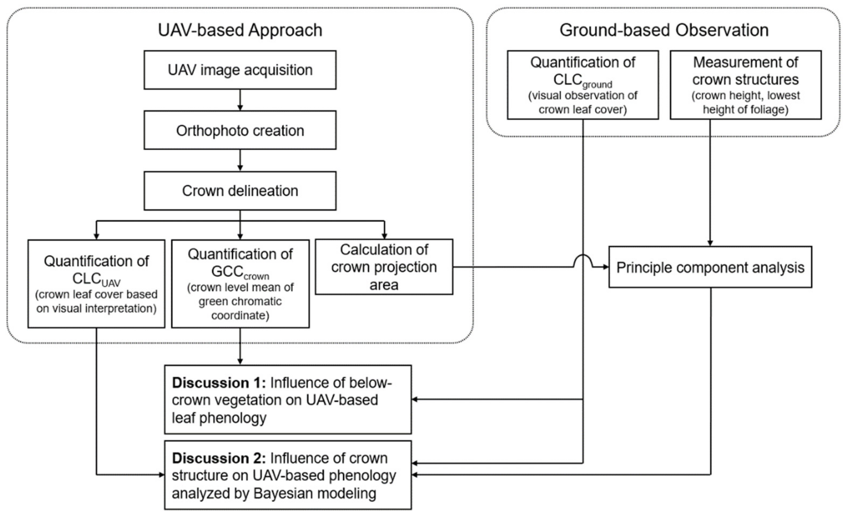
2.2.1. UAV-Based Observation

The aerial photographs were taken by a commercial drone (DJI Phantom 4 pro; DJI-Innovations Inc., Shenzen, China) equipped with a high-resolution camera. Prior to each UAV flight, the camera was configured for continuous shooting with the following settings: infinity focus; minimum focal length of 9 mm; and 16-megapixel resolution with super-fine compression. To minimize the effect of variable illumination on UAV image due to the solar incidence angle and cloud cover, the flights were conducted during midday (between 10 a.m. and 1 p.m.) on fine days. The UAV was flown at a height of about 15 m above the canopy surface (i.e., 35 m to 40 m above the ground surface) with manual operation. To achieve 80% of longitudinal and 50% of lateral overlapping for constructing an orthophoto by structure from motion (SfM) and multi-view stereopsis techniques, the UAV was operated at roughly 1.2 m s−1, with the camera taking images every 2 s. At least five flights were conducted over the 1.5 ha plot (25 min per flight) that collected between 2000 and 3000 JPEG images during each measurement occasion.
Each acquired image set was processed into a 5-cm resolution, georeferenced orthophoto using the Bentley ContextCapture software package (Bentley Systems Inc., Exton, PA, USA). The processing steps included automatic aerial triangulation, noise filtering, DSM and orthophoto creation. All of the processes were performed under default settings and in a fully automated way. As GPS information from the UAV was not accurate, the DSM and orthophoto was generated using the seven GCPs to enhance accuracy. However, during three occasions in November, orthophotos could not be created due to mechanic trouble with the UAV camera. Consequently, CLCUAV was estimated directly from the aerial JPEG image. The original JPEG images with a similar perspective as orthophotos were carefully chosen to minimize the error associated with using a JPEG image; thus, the same visual interpretation procedure (explained below) was applied in these instances (Figure S1).
We then made a crown polygon map for all of the individual trees in the canopy layer of the study plot with ArcGIS software (version 10.7, ESRI, Redlands, CA, USA). The boundaries of all crowns in the orthophoto were manually delineated based on the ground survey, and then linked each crown polygon to inventory data of the study plot, such as tree ID, species name, and diameter at breast height. The total number of digitized crowns was 650, but only 55 of these crowns were analyzed in the presented research.
With respect to CLCUAV, the percentage of leafy part in the target crown space was visually quantified at 5% intervals and then was classified using one of the following seven categories: 0%; 10% (1~19%); 30 % (20~39%); 50% (40~59%); 70% (60~79%); 90% (80~99%); and 100%. To facilitate the visual assessment, a time series of crown images was created by extracting the relevant area from each orthophoto (Figure S1). The leafy part of the target crown was carefully distinguished from that of the below-crown vegetation based on differences in phenology, brightness, color, and texture. Even in the study plot, which includes a multi-layered canopy structure, a human interpreter could easily identify the leafy part of a target crown in a fine-resolution UAV image (Figure S2). Therefore, the estimated CLCUAV values were not influenced by below-crown vegetation and represents the leaf phenology of the target crown.
The mean crown-level green chromatic coordinate (GCCcrown) for the 55 target crowns was calculated as:
GCC crown = G / R + G + B
where R, G, and B are the mean values of red, green, and blue digital numbers in the target crown space, respectively. In contrast to CLCUAV, GCCcrown is influenced by below-crown vegetation.
While the SfM approach has a number of advantages, crowns with a complex structure are difficult targets for accurate feature matching and architectural reconstruction. Although failed areas of reconstruction (indicated by a gray color in the orthoimage) were found in several images during leaf expansion and falling, the areas were generally small (Figure S1) and we excluded such areas from CLCUAV and GCCcrown calculations.

2.2.2. Ground-Based Observations

The observer looked at the target crowns from various directions with binoculars, and estimated the percentage of unfolding leaves and mean leaf size as the percentage of mature leaf size. The observer calculated crown leaf cover (CLCground) as a product of these two factors (Figure S3), and then categorized the result into one of the seven classes presented for CLCUAV. Since mature leaf size cannot be determined during leaf expansion based solely on ground observations, in situ visual estimates of the mean crown-level leaf size may be prone to human error. Therefore, photographs of the target crown were taken from the exact location where the observer had been on each occasion, and the mean leaf size derived from in situ visual observations was checked with that derived from the photographs after full-leaf expansion. Although we made adjustments to the leaf size for several trees, the visual estimates of observers were generally consistent with those derived from the photographs.

2.3. Crown Structural Traits

To analyze the effect of crown structure on the variations between CLCground and CLCUAV, crown height (CH), lowest foliage height (LH) and crown projection area (CA) were quantified for the 55 individual trees (Table 1). CH and LH were measured with a vertex hypsometer (Vertex IV, Haglöf, Sweden) in November 2019. CA was calculated from the digitized crowns in the orthophoto using ArcGIS software and, thus, represents the sunlit part of the crown. Crown length (CL) was calculated by subtracting LH from CH, and crown volume (CV) was calculated as a product of CA and CL. The ratio of CA and CL (CA/CL) was also determined as an index of relative crown length.

2.4. Data Analysis

To determine phenological transition dates (i.e., the start and end dates of leaf expansion and leaf falling) for each target tree, we fit the logistic curves to CLCground and CLCUAV data over time, respectively, representing both leaf expansion and leaf falling (108–212 DOY and 224–332 DOY, respectively), and defined the days that represented 5% and 95% of the maximum values of the fitted results as the start and end dates of leaf expansion, respectively (SOE and EOE, respectively) [9,24]. Moreover, the start and end dates of leaf falling (SOF and EOF, respectively) were determined to be the days representing 95% and 5% of the maximum values, respectively.
Growing season length was calculated as the difference between SOE and EOF. GCCcrown was only used to determine the phenological transition dates for the spring period, as the transition dates during leaf falling period were generally unclear across all of the studied species (Figure S4) and because orthophotos could not be constructed in November due to mechanical trouble with the UAV camera. Additionally, since most trees demonstrated a gradual decrease in GCC during the summer period (Figure S4), the logistic curve was fitted to data from 108 to 157–165 DOY, a time period when the decrease in GCC was not evident yet.
Multivariate associations between the crown structural traits (CH, CL, CA, CV, and CA/CL) were analyzed with a principal component analysis (PCA) using an individual tree to provide data points (Figure S5). The first two axes explained 94.7% (axis 1: 73.9%, axis 2: 20.8%) of the overall variation. CH, CL, CA, and CV were closely related to the first axis (Pearson correlation: CH: r = 0.84; CL: r = 0.91; CA: r = 0.95; CV: r = 0.96, all p < 0.001), while CA/CL was significantly related to the second axis (r = 0.80, p < 0.001). PCA was conducted with R version 3.6.2 (R Core Team 2019).
We adapted the hierarchical Bayesian framework to quantify the extent to which crown structure contributes to the variation between CLCUAV and CLCground. The relationship between CLCUAV and CLCground was first described using a simple linear model:
Logit (CLCUAVt) = a t, s · Logit (CLCgroundt) + b t, s
where:
Logit (CLC) = ln (CLC/ (100 − CLC))
CLC = 1, if CLC = 0
CLC = 99, if CLC = 100
Since CLC is discrete variable with a range between 0 and 100, logit transformation was applied. The parameters a and b describe the slope and intercept of the model, respectively. The subscripts of each variable and coefficient, namely, t and s, refer to individual tree and season (i.e., leaf expansion period in spring and leaf falling period in autumn), respectively. In this analysis, leaf expansion period was defined as the period when CLCground increases from 0% to 100% during the spring. Similarly, leaf falling period was defined as the period when CLCground decreases from 100% to 0% during the autumn. Instances in which both CLCUAV and CLCground were either 0% or 100% were excluded from the analysis. Number of data used in this analysis were 263 and 319 for leaf expansion period and leaf falling period, respectively. Secondly, since we hypothesize that the variations between CLCUAV and CLCground can be attributed to variation in the crown structures of individual trees (cf. the Introduction section), the slope and intercept of the linear model (Equation (2)) are described as;
at, s = c s · PC1 + d s · PC2 + e sp, s
bt, s = f s · PC1 + g s · PC2 + h sp, s
where PC1 and PC2 are the first and second axes of the PCA of crown structure, respectively (Figure S5). Each of the explanatory variables in Equations (3) and (4) was normalized to evaluate the relative contribution of each variable to the variations between CLCUAV and CLCground. The letters c~h are coefficients of the equations. Since other species-specific crown structure characteristics, such as leaf density and orientation, may also contribute to the variations between CLCUAV and CLCground, the coefficients e and h (i.e., intercepts of Equations (3) and (4)) were assumed to vary by species (subscript sp) in the full model. All coefficients were interconnected in this model framework and were obtained as probability distributions (hereafter, posterior distributions) at season, species, and individual tree level. Sampling from the posterior distributions of all parameters was performed using the Markov chain Monte Carlo (MCMC) method. We ran 40,000 iterations per each of the three independent MCMC chains after a warm-up of 20,000 iterations, with the chains thinned every five iterations to yield a posterior sample size of 12,000. The convergence of the Markov chains for each parameter was checked using R-hat values by comparing variance within each chain and among chains.
The contribution of crown structure to the variation between CLCUAV and CLCground was evaluated based on the Bayesian credible intervals (CIs) for the parameters c, d, f and g; i.e., if the 95% CI of the parameters did not cross zero, the parameter was regarded as significant. In addition, if the interquartile range of the posterior distribution of the parameter did not include zero, the parameter was considered to have a marginal significant effect. We compared a total of 32 models by removing the explanatory variables in Equations (3) and (4), and species variation of the coefficients e and h individually from the full model, and selected the best model that provided the lowest values of Watanabe–Akaike’s information criterion (WAIC). The Bayesian framework and related analyses were run in R version 3.6.2 using the rstan package.

3. Results

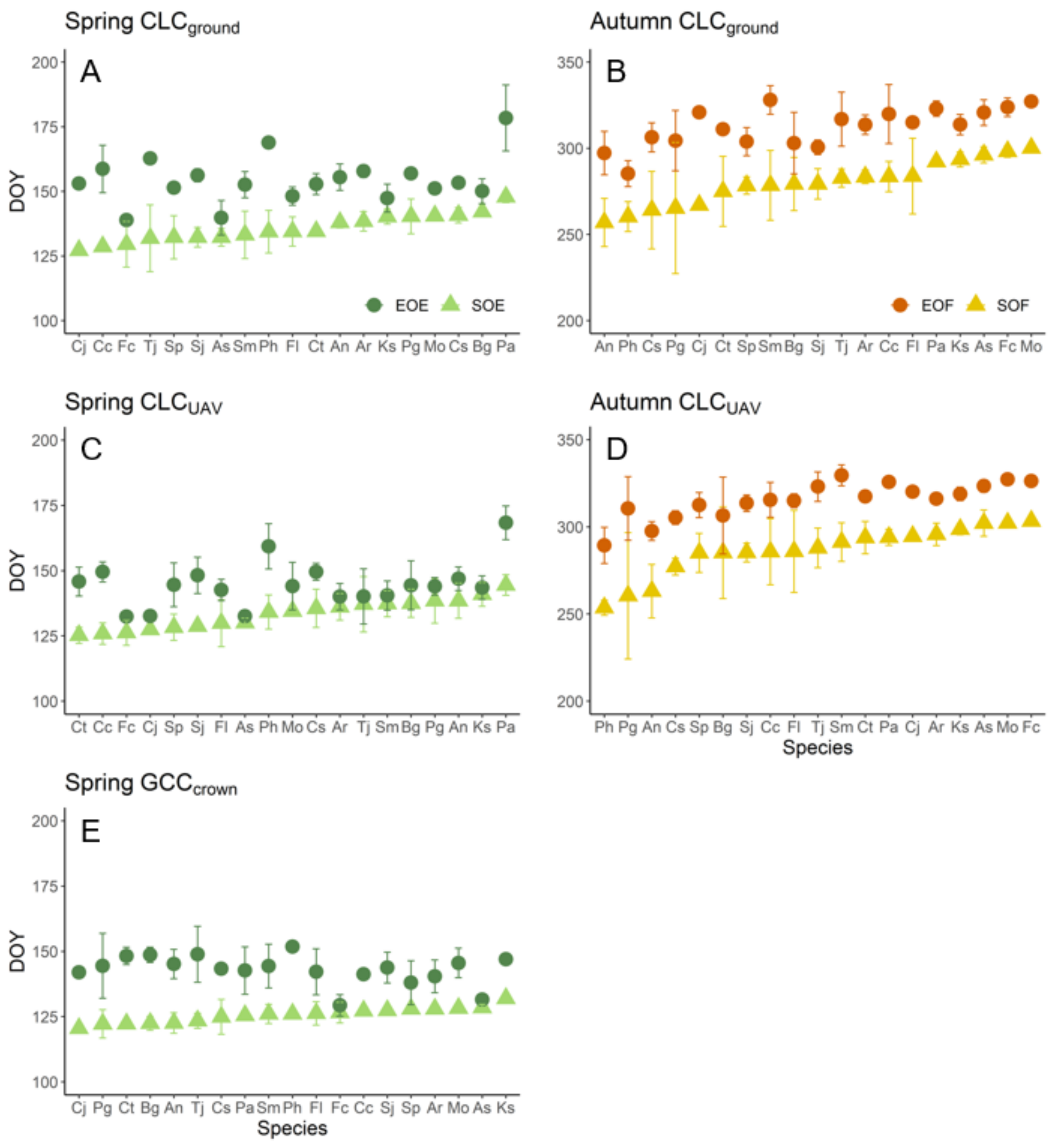
3.1. Inter-Species Differences in the Phenological Transition Dates Derived from the Ground Observations and UAV Images

Spring leaf phenology derived from crown leaf cover based on ground observation (CLCground) differed markedly among the species (Figure 2A). The mean start date of leaf expansion (SOE) varied by roughly three weeks among species, with Carpinus japonica showing the earliest SOE (DOY 127.2) and Phellodendron amurense showing the latest SOE (DOY 147.8). The mean end date of leaf expansion (EOE) showed larger inter-species variation than SOE, ranging from DOY 139.8 for Acer shirasawanum to DOY 178.4 for P. amurense (mean ± SD: 154.4 ± 9.9 DOY). As the studied species had different rank orders for EOE and SOE, the leaf expansion period (i.e., the difference between EOE and SOE) also varied between species, ranging from a minimum value of seven days for Kalopanax septemlobus to 34 days for Pterostyrax hispidus (mean ± SD: 18.1 ± 10.3 days). Autumn leaf phenology generally showed larger inter-species variation than spring leaf phenology (Figure 2B). More specifically, the mean start date of leaf falling (SOF) varied by six weeks among the species (mean ± SD: 279.1 ± 18.0 DOY); A. nipponicum had the earliest SOF (DOY 256.9), while Magnolia obovata had the latest SOF (DOY 300.2). The mean end date of leaf falling (EOF) also varied by six weeks across the species, ranging from DOY 285.3 for Pterostyrax hispidus to DOY 328.0 for Stewartia monadelpha. The species showed different rank orders for SOF and EOF, and the performed analysis revealed that the leaf falling period (i.e., the difference between EOF and SOF) was longer than the leaf expansion period, ranging from a minimum of 20 days for K. septemlobus to a maximum of 54 days for C. japonica (mean ± SD: 31.9 ± 16.2 days). Intra-species variations in the phenological transition dates were generally smaller than the inter-species variations, with the exception of Prunus grayana in the autumn.
Overall, the phenological transition dates derived from crown leaf cover determined by the visual interpretation of UAV images (CLCUAV) showed similar trends with those derived from CLCground (Figure 2C,D). Consequently, significant correlations between CLCUAV- and CLCground-derived transition dates were consistently found throughout the growing seasons, with the best matches occurring for SOE (RMSE = 6.4, Figure 3A–D). However, the RMSE values of the relationships for EOE and SOF were larger than those for SOE and EOF by approximately six days. Consequently, although the CLCUAV-derived growing season period (the difference between EOF and SOE) was closely associated with the CLCground-derived growing season period, large mismatches were found for the period of leaf expansion and leaf falling (Figure 3E–G).
The SOE and EOE derived from mean crown-level green chromatic coordinate (GCCcrown) generally occurred at an earlier time point than those derived from CLCground irrespective of species (Figure 2E). Additionally, the inter-species variations in the GCCcrown-derived transition dates were substantially smaller than those in the CLCground-derived transition dates (mean ± SD: 126.6 ± 3.5 and 140.5 ± 6.4 DOY, respectively). Consequently, the phenological transition dates and leaf expansion periods derived from GCCcrown were poorly correlated with those derived from CLCground (Figure 3A,B,E).

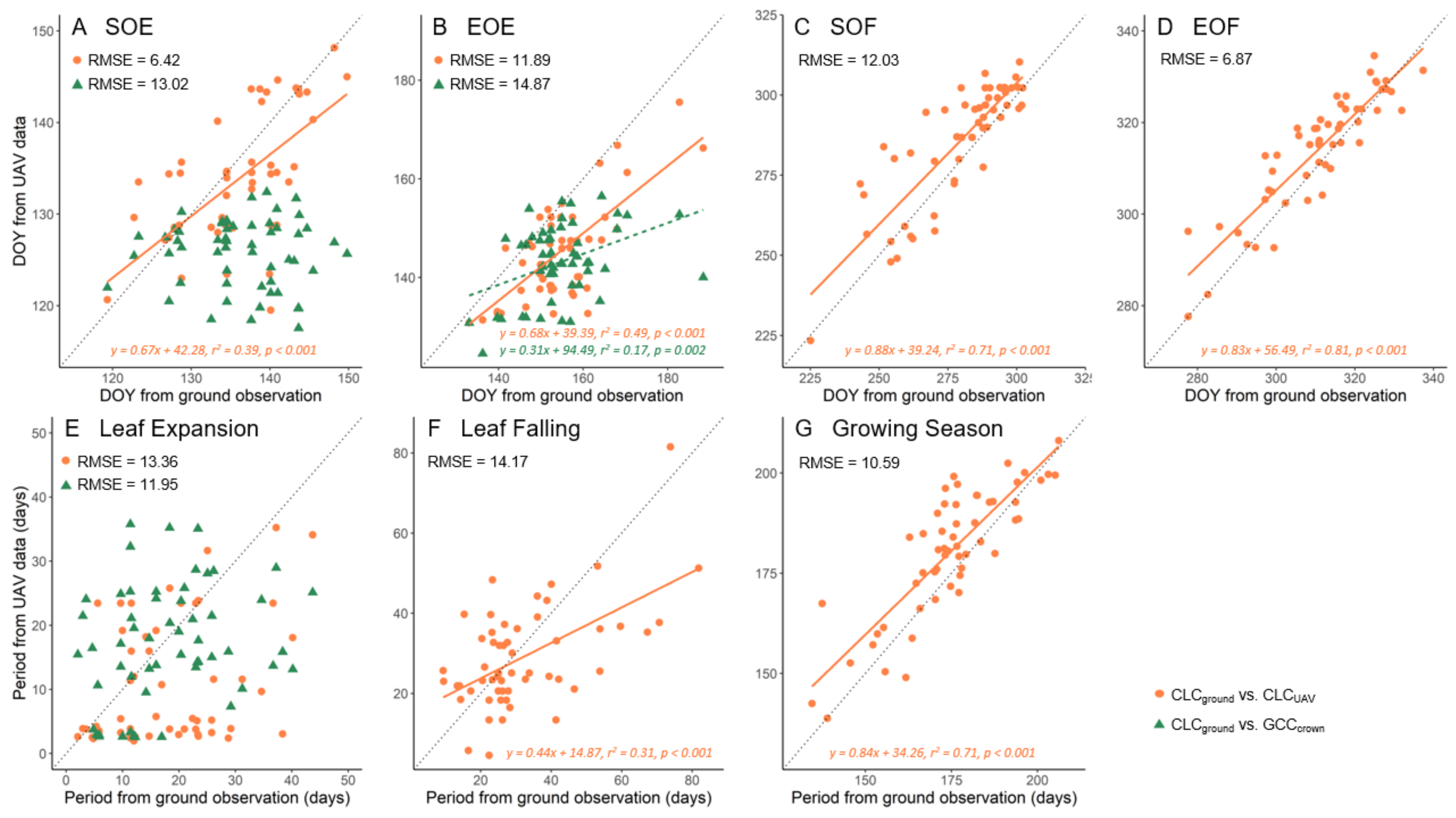
3.2. Direct Comparison of the Phenological Metrics Derived from UAV Data and Ground Observations

In general, CLCUAV increased earlier than CLCground during spring leaf expansion (Figure 4). However, the degree of variation between CLCUAV and CLCground markedly differed among species; e.g., considerable variations were found for Acer rufinerve, A. shirasawanum, and Fagus crenata, while the variations were relatively small for Cornus controvesa, Fraxinus lanuginosa, P. amurense, and P. hispidus. A similar discrepancy between CLCUAV and CLCground was also found in autumn, but the variation was generally smaller than what was observed in the spring, especially for late successional species, such as A. shirasawanum, F. crenata, and T. japonica (Figure 4B). Relative GCCcrown showed similar trends with CLCUAV in the spring, but increased more rapidly than CLCUAV for some species, such as Acer nipponicum and P. amurense (Figure 4A). The differences between CLCground-derived SOE and GCCcrown-derived SOE were positively correlated with CLCground-derived SOE (Figure 5), indicating that GCCcrown errors are larger for species with a later SOE.

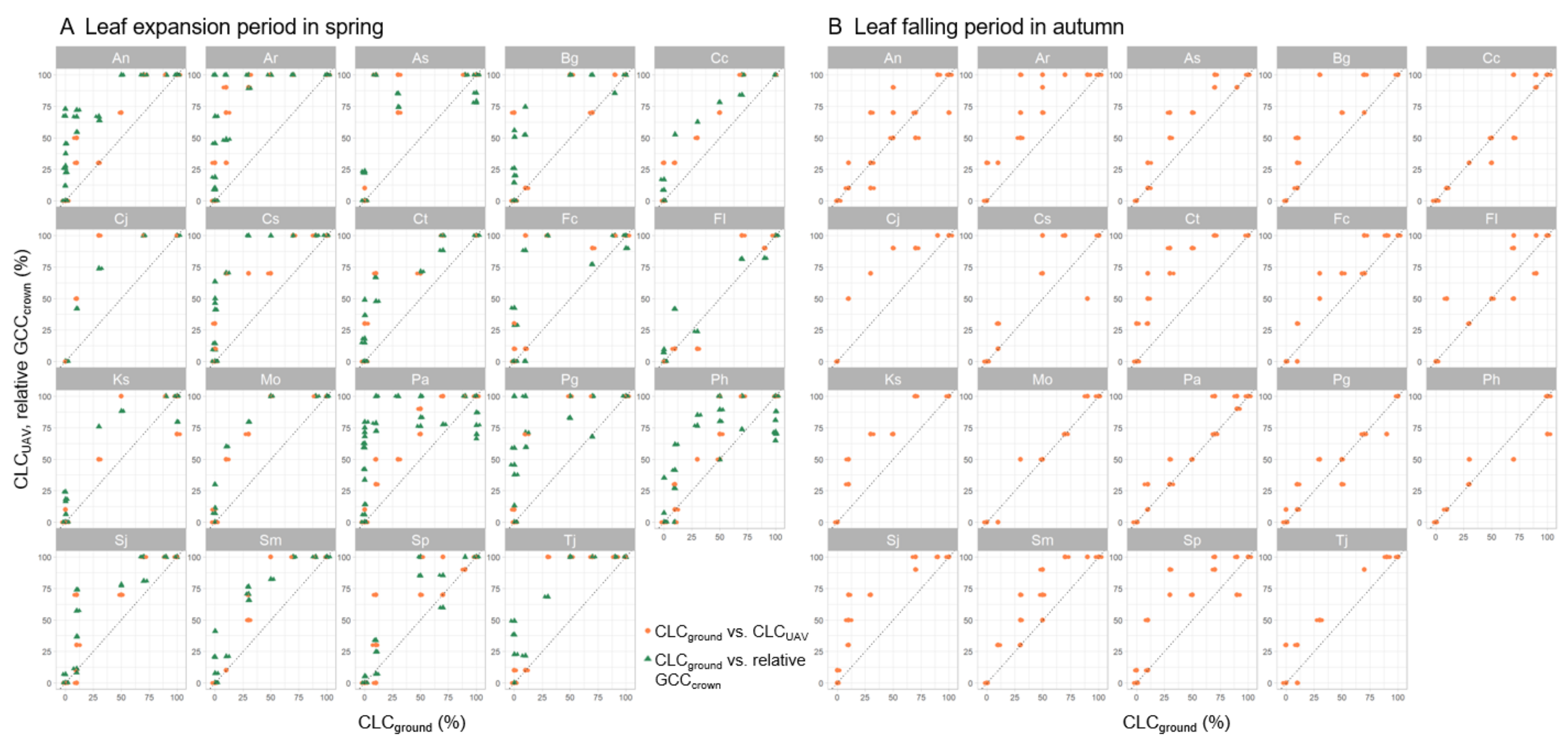
3.3. Contribution of Crown Structure to the Discrepancy between CLCUAV and CLCground

The extent to which crown structure contributed to the discrepancy between CLCUAV and CLCground was examined through the selection of a hierarchical Bayesian model (Equations (2)–(4)) based on WAIC. The top five models with the best results, as well as one model including inter-species variations, are shown in Table 2. The median value of coefficient h in Equation (4) was about two-fold higher in the spring than in the autumn irrespective of the model. This can be explained by the fact that variations between CLCUAV and CLCground were generally larger in the spring than in the autumn (Figure 4). In contrast, the median value of coefficient e in Equation (3) was fairly constant at around 1.0 irrespective of the season. Both coefficients e and h were assumed to vary with species (No.6); the median value of coefficient h varied markedly across species whereas the value of coefficient e was stable at around 1.0 for all species. However, since the interquartile ranges of coefficient h for the studied species showed a certain degree of overlap (results not shown), the model including species variation showed higher WAIC values than the model that did not include this variation. This result implies that variation between CLCUAV and CLCground occurs at the individual tree-level but not at the species-level. In the model with the best fit, the first PCA axis (PC1, Figure S5) exerted a significantly positive effect on the parameter b in the spring, but this significant effect was not detected in the autumn. Although marginally significant effects were found for both parameters a and b in the autumn, they demonstrated opposing effects, indicating that crown structure had only a minor influence on the variation between CLCUAV and CLCground in the autumn. The significant positive effect of PC1 on parameter b was consistently found in the top five models.

4. Discussion

Ground-based observations of crown leaf phenology demonstrated clear spatial heterogeneity at the study site; more specifically, intra- and inter-species variations in the phenological transition dates were up to ~20 days during the spring and ~40 days during the autumn. This unequal leaf expansion and falling agree with shoot and crown-level observations from other cool temperate forests in Japan (e.g., [25,26,27,28]). The start dates of leaf expansion (SOE) and end dates of leaf falling (EOF) derived from crown leaf cover determined by visual interpretation of UAV images (CLCUAV) were associated with those derived from crown leaf cover based on ground observation (CLCground) across all 19 studied tree species, with an accuracy of about six days (Figure 3). This result suggests that UAV observation is an effective method for quantifying growing season length at the individual tree scale in deciduous forests. However, it is important to note that the influence of below-crown vegetation, such as understory vegetation, subcanopy trees and branches of neighboring trees, were excluded from CLCUAV by the visual discrimination of this vegetation from the UAV images (Figure S2). When mean crown-level green chromatic coordinate (GCCcrown)—the most commonly used metric for quantifying leaf phenology in near-surface remote-sensing—was used to estimate the phenological transition dates, inter- and intra-species variation in spring leaf phenology was poorly explained (Figure 3A,B,E). This was particularly noticeable for species with a later SOE (Figure 5), which suggests that below-crown vegetation significantly hampers the estimation of crown leaf phenology with UAV imaging. The study site has rather sparse understory vegetation relative to other cool temperate forests in Japan because of the continuous and excessive browsing by Sika deer, along with the mass flowering and die-off event of dwarf bamboo, which occurred three years before the experiments. However, a certain number of shrubs and saplings which survived from bark stripping by deer still remained in the subcanopy layer (ca. 5~15 m). These young trees of the subcanopy layer tend to have earlier leaf emergence than mature trees in the canopy layer mainly due to ontogenetic differences in leaf phenology [12,29]. Additionally, branches of neighboring trees frequently invaded the crown space of the target tree, which could be expected to increase the discrepancy between GCCcrown and CLCUAV when the neighboring trees have an earlier SOE than the target tree (Figure S2). It can be theorized that if the study site is not exposed to excessive deer browsing and a die-off event of dwarf bamboo, then even more substantial discrepancies between the GCCcrown- and CLCUAV-derived SOE and EOE would be observed. Thus, the influence of below-crown vegetation needs to be removed first whenever a UAV-based approach is applied to a multi-layered forest, like the study site of the present paper.
The CLCUAV-derived end date of leaf expansion (EOE) and start date of leaf falling (SOF) were less accurate than SOE and EOF (Figure 3). On average, CLCUAV-derived EOE preceded the result derived from CLCground by 12 days; conversely, CLCUAV-derived SOF was 12 days later than the result derived from CLCground. With respect to the EOE discrepancy, a similar result was reported from a study which used a tower-mounted phenocam in a temperate deciduous broad-leaved forest; the spring peak for canopy-level green chromatic coordinate occurred about two weeks before that of the ground-observed leaf size and leaf area index (LAI) [10]. The authors attributed this discrepancy in the spring peak to the oblique viewing angle of the phenocam, i.e., the near-horizontal-oriented camera captures more leaf layers of canopy trees than the nadir viewing angle (e.g., UAV camera), leading to higher effective LAI and a faster increase in GCC than actual changes in LAI. However, the results presented in this paper revealed that nadir photography approaches can also yield an earlier detection of the spring peak even when the influence of below-crown vegetation is removed. Furthermore, Bayesian model analysis indicated that the spring variation between values derived from CLCUAV and CLCground increase as crown size, e.g., crown length and volume, increases (Table 2, Figure S5). This suggests that the earlier saturation of CLCUAV and GCC is a result of leaf overlapping within the crown, as the nadir viewing angle of the UAV camera will capture more leaf layers for large and thick crowns than for small and thin crowns.
The discrepancies between CLCUAV and CLCground were especially large for late-successional, shade-tolerant species, such as Fagus crenata, A. shirasawanum, and Tilia japonica, relative to early successional, shade intolerant species, such as Pterostyrax hispidus and Phellodendron amurense, during leaf expansion period (Figure 4). Although the Bayesian model analysis did not provide evidence that interspecies variation contributes to the observed discrepancies between CLCUAV and CLCground, the result above does not contradict the finding that CLCUAV error increases with crown size because late-successional, shade-tolerant species tend to form a multi-layered crown, while early-successional, shade-intolerant species form a mono-layered crown ([20,21,30], Figure S5). Hagemeier and Leuschner [31] found that the late-successional species of European temperate forests have a larger crown LAI than early-successional species due to high leaf area density in the upper layer. Furthermore, the late-successional species form extended leaf layers with nearly horizontal leaf orientation in the lower layer. Therefore, changes in not only the outside crown structure, but also the interior structure, (e.g., leaf distribution and orientation), may contribute to the large discrepancies between CLCUAV and CLCground noted for late-successional species.
CLCUAV was also larger than CLCground for most of the studied species during the autumn leaf falling period (Figure 4). However, for the late-successional species, such as A. shirasawanum, F. crenata, and T. japonica, the degree of variation between CLCUAV and CLCground was markedly smaller than what was observed for springtime measurements. Consequently, crown structure did not significantly contribute to the variation between CLCUAV and CLCground during the fall (Table 2). In late-successional species, leaf falling starts from the upper parts of the crown [32]. Since most of the leaves in the crown are concentrated in the upper part, such unequal leaf falling should generate large gaps within the crown that can be detectable in UAV images. In contrast, springtime leaf emergence occurs consistently throughout the crown in late-successional species [32]. Since leaf emergence finished 1–2 weeks earlier than leaf expansion for most of the studied species, mean crown-level leaf size was a predominant factor for the springtime CLCground trajectory ([18], Figure S3). The even distribution of small leaves throughout the crown will mean that few gaps remain in the UAV images of large and thick crowns due to high leaf overlapping and, subsequently, result in the large discrepancy between CLCUAV and CLCground (Figure S3). Therefore, spatial variations in leaf emergence and falling may partially explain why the error in CLCUAV varied by season, and was especially noticeable in late-successional species. Research including tower-mounted phenocams has reported that the normalized difference vegetation index (NDVI) is more sensitive to changes in canopy LAI than the greenness derived from digital camera images. This is because NDVI incorporates bands at near-infrared (NIR) wavelengths, at which the reflectance of leaves is strongly governed by structural characteristics rather than pigmentation [33]. Therefore, the use of an UAV equipped with a NIR camera may solve the problem of early saturation of phenological metrics during the spring. Although Berra et al. [17] showed that UAV-derived NDVI was less successful in predicting phenological transition date than GCC in mixed deciduous and conifer woodland, the result was based on erroneous estimates of NDVI that integrated RGB and NIR images that had been captured individually by two different UAVs. Since UAVs equipped with a multispectral sensor are commercially available, it would be valuable to monitor NDVI with a single UAV in future research.
Since visual assessments are always prone to human error, it could be expected that the observed discrepancy between CLCUAV and CLCground can be attributed to human error in the interpretation of UAV images and/or in situ crown leaf cover. For species with an earlier SOE, such as Carpinus tschonoskii, Cornus controversa, and F. crenata, the influence of below-crown vegetation on the visual interpretation of UAV images was marginal. This is because the timing of leaf emergence in these species is almost simultaneous with, or even earlier than, the below-crown vegetation. This is evident from the fact that SOE derived from GCCcrown was similar to the result derived from CLCUAV (Figure 2C,E). In such species, the springtime GCCcrown—which is more objective than visual interpretation—showed a similar trend with CLCUAV, and sometimes showed a more rapid increase than CLCUAV (Figure S4). This suggests that errors stemming from the visual interpretation of UAV images are likely small, and using GCCcrown in estimations would lead to larger variations in crown leaf phenology than using CLCUAV. Park et al. [3] showed that the human interpretation of UAV images could yield largely repeatable CLCUAV values for a lowland moist tropical forest. This research included different observers who had not received specific training to standardize their interpretations, a characteristic which supports our conclusion. With respect to ground-based visual observations in a dense and multi-layered forest, human error will be high as the observers cannot see the whole crown of the target tree. To minimize this error, we carefully selected trees for which both the upper and lower parts of the crown were visible from the ground through gaps around the target trees. Additionally, mean crown-level leaf size, which is a major component of the springtime CLCground, was validated with a semi-objective approach; more specifically, the scores determined in the field were checked using foliage photographs that had been taken from the ground by a digital camera (Figure S3 inset photographs). Therefore, we concluded that the observed variations between CLCUAV and CLCground are not solely due to human error during the visual assessment.
However, it should be noted that the accuracy of the UAV-based approach depends on the temporal frequency of UAV data acquisition dates, which is similar to ground-based observations. Schwartz et al. [34] showed that the accuracy of ground observations decreased when the observation interval was greater than four days, for deciduous tree species in the sub-boreal forest. Therefore, the relatively long interval of this study (5–10 days) may cause uncertainty for the prediction of phenological metrics and subsequent calculation of the transition dates and analyses with Bayesian modeling. In addition, leaf phenology and crown structure show large inter-annual variations due to various events, such as late spring frost, heavy fruiting, and the outbreak of defoliating insects (e.g., [35,36,37]). Therefore, only one year of observation of this study may be too short to cover the inter- and intra-species variations in leaf phenology and crown structure. To enhance the generic applicability of this study’s result, further data accumulation by more frequent observation and long-term monitoring is necessary.

5. Conclusions

We showed that UAV-based observation is a powerful approach for quantifying the start and end of the growing season at an individual tree scale in a forest containing various species when the influence of subcanopy trees and understory vegetation is small, or can be readily eliminated with data processing. However, the UAV-based approach provided a markedly earlier EOE date in comparison to ground observations. Results from the Bayesian modeling suggest that EOE error increases as crown size (crown length and volume) increases, and is most probably explained by high leaf overlapping within the crown. Since crown structure varies with various factors such as species, light environment, ontogeny and competition, the effect of crown structure on the UAV-derived phenological metrics needs to be considered to ensure accurate estimates of individual tree phenology. This type of insight will be important for bridging the performance of UAV-based approaches and traditional ground-based observation.

Supplementary Materials

The following are available online at https://0-www-mdpi-com.brum.beds.ac.uk/article/10.3390/f12040425/s1. Figure S1: Example of a time-series of UAV images used for the visual interpretation; Figure S2: Images demonstrating the influence of below-crown vegetation; Figure S3: Comparison of spring trajectories for mean crown leaf size, frequency of unfolding leaves, ground-based crown leaf cover and UAV-derived crown leaf cover; Figure S4: Time series of crown leaf cover based on ground observation, crown leaf cover determined by visual interpretation of UAV images, and mean crown green chromatic coordinate; Figure S5: Principal component analysis (PCA) for the crown structural parameters.

Author Contributions

Conceptualization: A.I.; data curation: N.B.; formal analysis: N.B.; funding acquisition: A.I.; investigation: N.B.; methodology: N.B., H.M. and A.I.; project administration: A.I.; resources: A.I.; supervision: A.I.; visualization: N.B.; writing—original draft: N.B.; writing—review and editing: H.M. and A.I. All authors have read and agreed to the published version of the manuscript.

Funding

This research was funded by KAKENHI (18H02236; Grant-in-Aid for Scientific Research B by the Japan Society for the Promotion of Science).

Institutional Review Board Statement

Not applicable.

Informed Consent Statement

Not applicable.

Data Availability Statement

The data presented in this study are available on request from the corresponding author. The data are not publicly available due to ongoing analysis for other publication.

Acknowledgments

The authors thank Quan Wang of Shizuoka University for his critical comments, and the students of the Silviculture Laboratory of Shizuoka University who assisted with field research. N. Budianti was supported by the English special program of Gifu University.

Conflicts of Interest

The authors declare no conflict of interest.

Abbreviations

CACrown area
CA/CLRatio of CA to crown length
CHCrown height
CLCrown length
CVCrown volume
CLCgroundCrown leaf cover determined from ground observation
CLCUAVCrown leaf cover determined from visual interpretation of UAV images
EOEEnd date of leaf expansion
EOFEnd date of leaf falling
GCCcrownMean crown-level green chromatic coordinate derived from UAV image
LAILeaf area index
SOEStart date of leaf expansion
SOFStart date of leaf falling
UAVUnmanned aerial vehicle

References

  1. Richardson, A.D.; Keenan, T.F.; Migliavacca, M.; Ryu, Y.; Sonnentag, O.; Toomey, M. Climate change, phenology, and phenological control of vegetation feedbacks to the climate system. Agric. For. Meteorol. 2013, 169, 156–173. [Google Scholar] [CrossRef]
  2. Klosterman, S.; Richardson, A.D. Observing spring and fall phenology in a deciduous forest with aerial drone imagery. Sensors 2017, 17, 2852. [Google Scholar] [CrossRef] [PubMed] [Green Version]
  3. Park, J.Y.; Muller-Landau, H.C.; Lichstein, J.W.; Rifai, S.W.; Dandois, J.P.; Bohlman, S.A. Quantifying leaf phenology of individual trees and species in a tropical forest using unmanned aerial vehicle (UAV) images. Remote Sens. 2019, 11, 1534. [Google Scholar] [CrossRef] [Green Version]
  4. Richardson, A.D.; Braswell, B.H.; Hollinger, D.Y.; Jenkins, J.P.; Ollinger, S.V. Near-surface remote sensing of spatial and temporal variation in canopy phenology. Ecol. Appl. 2009, 19, 1417–1428. [Google Scholar] [CrossRef] [PubMed]
  5. Sonnentag, O.; Hufkens, K.; Teshera-Sterne, C.; Young, A.M.; Friedl, M.; Braswell, B.H.; Milliman, T.; O’Keefe, J.; Richardson, A.D. Digital repeat photography for phenological research in forest ecosystems. Agric. For. Meteorol. 2012, 152, 159–177. [Google Scholar] [CrossRef]
  6. Ahrends, H.E.; Bräugger, R.; Stöckli, R.; Schenk, J.; Michna, P.; Jeanneret, F.; Wanner, H.; Eugster, W. Quantitative phenological observations of a mixed beech forest in northern Switzerland with digital photography. J. Geophys. Res. Biogeosci. 2008, 113, 1–11. [Google Scholar] [CrossRef] [Green Version]
  7. Richardson, A.D.; Hollinger, D.Y.; Dail, D.B.; Lee, J.T.; Munger, J.W.; O’Keefe, J. Influence of spring phenology on seasonal and annual carbon balance in two contrasting New England forests. Tree Physiol. 2009, 29, 321–331. [Google Scholar] [CrossRef]
  8. Migliavacca, M.; Sonnentag, O.; Keenan, T.F.; Cescatti, A.; O’Keefe, J.; Richardson, A.D. On the uncertainty of phenological responses to climate change, and implications for a terrestrial biosphere model. Biogeosciences 2012, 9, 2063–2083. [Google Scholar] [CrossRef] [Green Version]
  9. Hufkens, K.; Friedl, M.; Sonnentag, O.; Braswell, B.H.; Milliman, T.; Richardson, A.D. Linking near-surface and satellite remote sensing measurements of deciduous broadleaf forest phenology. Remote Sens. Environ. 2012, 117, 307–321. [Google Scholar] [CrossRef]
  10. Keenan, T.F.; Darby, B.; Felts, E.; Sonnentag, O.; Friedl, M.A.; Hufkens, K.; O’Keefe, J.; Klosterman, S.; Munger, J.W.; Toomey, M.; et al. Tracking forest phenology and seasonal physiology using digital repeat photography: A critical assessment. Ecol. Appl. 2014, 24, 1478–1489. [Google Scholar] [CrossRef] [Green Version]
  11. Mizunuma, T.; Wilkinson, M.; Eaton, E.L.; Mencuccini, M.; Morison, J.I.L.; Grace, J. The relationship between carbon dioxide uptake and canopy colour from two camera systems in a deciduous forest in southern England. Funct. Ecol. 2013, 27, 196–207. [Google Scholar] [CrossRef]
  12. Seiwa, K. Changes in leaf phenology are dependent on tree height in Acer mono, a deciduous broad-leaved tree. Ann. Bot. 1999, 83, 355–361. [Google Scholar] [CrossRef] [Green Version]
  13. Augspurger, C.K.; Cheeseman, J.M.; Salk, C.F. Light gains and physiological capacity of understorey woody plants during phenological avoidance of canopy shade. Funct. Ecol. 2005, 19, 537–546. [Google Scholar] [CrossRef]
  14. Lopez, O.R.; Farris-Lopez, K.; Montgomery, R.A.; Givnish, T.J. Leaf phenology in relation to canopy closure in southern Appalachian trees. Am. J. Bot. 2008, 95, 1395–1407. [Google Scholar] [CrossRef]
  15. Richardson, A.D.; O’Keefe, J. Phenological Differences between Understory and Overstory: A Case Study Using the Long-Term Harvard Forest Records. In Phenology of Ecosystem Processes: Applications in Global Change Research; Noormets, A., Ed.; Springer: New York, NY, USA, 2009; pp. 87–117. ISBN 978-1-4419-0025-8. [Google Scholar]
  16. Gressler, E.; Jochner, S.; Capdevielle-Vargas, R.M.; Morellato, L.P.C.; Menzel, A. Vertical variation in autumn leaf phenology of Fagus sylvatica L. in southern Germany. Agric. For. Meteorol. 2015, 201, 176–186. [Google Scholar] [CrossRef]
  17. Berra, E.F.; Gaulton, R.; Barr, S. Assessing spring phenology of a temperate woodland: A multiscale comparison of ground, unmanned aerial vehicle and Landsat satellite observations. Remote Sens. Environ. 2019, 223, 229–242. [Google Scholar] [CrossRef]
  18. Klosterman, S.T.; Hufkens, K.; Gray, J.M.; Melaas, E.; Sonnentag, O.; Lavine, I.; Mitchell, L.; Norman, R.; Friedl, M.A.; Richardson, A.D. Evaluating remote sensing of deciduous forest phenology at multiple spatial scales using PhenoCam imagery. Biogeosciences 2014, 11, 4305–4320. [Google Scholar] [CrossRef] [Green Version]
  19. Xie, Y.; Civco, D.L.; Silander, J.A. Species-specific spring and autumn leaf phenology captured by time-lapse digital cameras. Ecosphere 2018, 9, 1–21. [Google Scholar] [CrossRef] [Green Version]
  20. Valladares, F.; Niinemets, Ü. Shade Tolerance, a Key Plant Feature of Complex Nature and Consequences. Annu. Rev. Ecol. Evol. Syst. 2008, 39, 237–257. [Google Scholar] [CrossRef] [Green Version]
  21. Niinemets, Ü. A review of light interception in plant stands from leaf to canopy in different plant functional types and in species with varying shade tolerance. Ecol. Res. 2010, 25, 693–714. [Google Scholar] [CrossRef]
  22. Mizunaga, H.; Fujii, K. Is foliage within crowns of Cryptomeria japonica more heterogeneous and clumpy with age? J. Sustain. For. 2013, 32, 266–285. [Google Scholar] [CrossRef]
  23. Niinemets, Ü.; Valladares, F. Tolerance to shade, drought, and waterlogging of temperate northern hemisphere trees and shrubs. Ecol. Monogr. 2006, 76, 521–547. [Google Scholar] [CrossRef]
  24. Zhang, X.; Friedl, M.A.; Schaaf, C.B.; Strahler, A.H.; Hodges, J.C.F.; Gao, F.; Reed, B.C.; Huete, A. Monitoring vegetation phenology using MODIS. Remote Sens. Environ. 2003, 84, 471–475. [Google Scholar] [CrossRef]
  25. Kikuzawa, K. Leaf survival of woody plants in deciduous broad-leaved forests. 1. Tall trees. Can. J. Bot. 1983, 61, 2133–2139. [Google Scholar] [CrossRef]
  26. Aoki, Y.; Hashimoto, R. Leaf phenology of woody plant species in a cool-temperate secondary forest of Quercus serrata. Bull. Iwate Univ. For. 1995, 26, 29–41. [Google Scholar]
  27. Kato, S.; Yamamoto, M.; Komiyama, A. Leaf phenology of over-and understory trees in a deciduous broad-leaved forest: An observation at the Mumai plot in 1997. Japan J. For. Environ. 1999, 41, 39–44. [Google Scholar]
  28. Aikawa, T.; Tateno, R.; Takeda, H. Leaf phenology along a slope in a cool temperate deciduous forest. For. Res. Kyoto 2002, 74, 21–33. [Google Scholar]
  29. Vitasse, Y. Ontogenic changes rather than difference in temperature cause understory trees to leaf out earlier. New Phytol. 2013, 198, 149–155. [Google Scholar] [CrossRef] [PubMed]
  30. Larcher, W. Physiological Plant Ecology: Ecophysiology and Stress Physiology of Functional Groups, 4th ed.; Springer: Berlin/Heidelberg, Germany, 2003. [Google Scholar]
  31. Hagemeier, M.; Leuschner, C. Functional crown architecture of five temperate broadleaf tree species: Vertical gradients in leaf morphology, leaf angle, and leaf area density. Forests 2019, 10, 265. [Google Scholar] [CrossRef] [Green Version]
  32. Koike, T. Autumn coloring, photosynthetic performance and leaf development of deciduous broad-leaved trees in relation to forest succession. Tree Physiol. 1991, 7, 21–32. [Google Scholar] [CrossRef] [PubMed]
  33. Brown, L.A.; Dash, J.; Ogutu, B.O.; Richardson, A.D. On the relationship between continuous measures of canopy greenness derived using near-surface remote sensing and satellite-derived vegetation products. Agric. For. Meteorol. 2017, 247, 280–292. [Google Scholar] [CrossRef] [Green Version]
  34. Schwartz, M.D.; Hanes, J.M.; Liang, L. Comparing carbon flux and high-resolution spring phenological measurements in a northern mixed forest. Agric. For. Meteorol. 2013, 169, 136–147. [Google Scholar] [CrossRef]
  35. Hall, R.J.; Fernandes, R.A.; Hogg, E.H.; Brandt, J.P.; Butson, C.; Case, B.S.; Leblanc, S.G. Relating aspen defoliation to changes in leaf area derived from field and satellite remote sensing data. Can. J. Remote Sens. 2003, 29, 299–313. [Google Scholar] [CrossRef]
  36. Hufkens, K.; Friedl, M.A.; Keenan, T.F.; Sonnentag, O.; Bailey, A.; O’Keefe, J.; Richardson, A.D. Ecological impacts of a widespread frost event following early spring leaf-out. Glob. Change Biol. 2012, 18, 2365–2377. [Google Scholar] [CrossRef]
  37. Iio, A. Masting changes canopy structure, light interception, and photosynthesis in Fagus crenata. In Proceedings of the 7th International Conference on Functional-Structural Plant Models, Saariselkä, Finland, 9–14 June 2013; p. 174. [Google Scholar]
Figure 1. Workflow of data acquisition and analysis (details in Section 2).
Forests 12 00425 g001
Figure 2. Inter-species differences in the phenological transition dates derived from the three different metrics: (A,B) crown leaf cover based on ground observations (CLCground); (C,D) crown leaf cover determined by visual interpretation of the UAV images (CLCUAV); and (E) mean crown-level green chromatic coordinate calculated from the UAV images (GCCcrown). Each data point represents the mean value (±SD) of the phenological transition date. Other abbreviations: SOE—start date of leaf expansion; EOE—end date of leaf expansion; SOF—start date of leaf falling; EOF—end date of leaf falling. Species abbreviations are shown in Table 1. The x-axis of each panel is sorted by either SOE or SOF.
Forests 12 00425 g002
Figure 3. Comparison of phenological transition dates and periods derived from crown leaf cover based on ground observation (CLCground) and UAV data (i.e., crown leaf cover determined by visual interpretation of UAV images; CLCUAV, and mean crown-level green chromatic coordinate calculated from the UAV images; GCCcrown). Each point represents data for an individual tree. Other abbreviations: SOE—start date of leaf expansion; EOE—end date of leaf expansion; SOF—start date of leaf falling; EOF—end date of leaf falling. The dotted line indicates a 1:1 relationship, and thick lines are regression equations (details in the lower part of each panel).
Forests 12 00425 g003
Figure 4. Direct comparison of crown leaf cover based on ground observation (CLCground) with the phenological metrics derived from UAV data during: (A) leaf expansion in the spring (108–212 DOY); and (B) leaf falling in the autumn (224–332 DOY). Each point represents raw data from a single tree at each measurement occasion. Jitter was added to data points that lay on the same percentage, with the dotted line showing a 1:1 relationship. Abbreviations: CLCUAV—crown leaf cover based on visual interpretation of UAV images; GCCcrown—mean crown-level green chromatic coordinate calculated from the UAV images. Abbreviations of the species names are clarified in Table 1. GCCcrown was converted to the same scale as crown leaf cover to enable direct comparisons, i.e., the minimum GCCcrown before bud break was set to 0% and the spring GCCcrown peak was set to 100% (relative GCCcrown). Seasonal pattern of each phenological metric is shown in Figure S4.
Forests 12 00425 g004
Figure 5. Association between the start date of leaf expansion (SOE) derived from crown leaf cover based on ground observation (CLCground) and the difference between mean crown level green chromatic coordinate (GCCcrown) and CLCground-derived SOE. Each point represents an individual tree, and the solid line denotes the regression relationship.
Forests 12 00425 g005
Table 1. List of species, including crown structure and successional type, used in the research. The species successional type was determined based on the regeneration status of seedlings in the canopy gaps at the study plot (personal observation) and the database for shade tolerance by Niinemets and Valladares [23]. Species for which regeneration status could not be confirmed in the study plot were classified as “Unknown”. Abbreviations: DBH—the diameter at breast height; H—tree height; CA—crown projection area; CL—crown length.
No.Species NameSpecies CodeNumber of SamplesDBH (cm)H (m)CA (m2)CL (m)Successional Type
1.Acer nipponicumAn520.13–53.8114.75–20.4014.63–80.904.93–10.90Unknown
2.Acer rufinerveAr441.80–52.8714.25–20.8520.30–51.544.85–11.85Mid
3.Acer shirasawanumAs342.44–76.6017.15–21.1053.10–83.159.40–10.50Late
4.Betula grossaBg331.80–34.9017.35–18.9737.44–81.598.30–11.17Early
5.Carpinus japonicaCj126.7515.4527.676.5Mid
6.Carpinus tschonoskiiCt330.78–37.4814.35–27.824.29–45.445.00–13.10Mid
7.Chengiopanax sciadophylloidesCs334.62–41.5016.65–19.9016.51–39.827.30–9.15Mid
8.Cornus controversaCc222.63–55.2113.50–20.955.55–111.773.20–11.35Mid
9.Fagus crenataFc345.75–59.4623.00–32.3571.35–132.0914.10–23.10Late
10.Fraxinus lanuginosaFl323.22–32.4714.35–16.0527.73–52.094.05–6.45Mid
11.Kalopanax septemlobusKs329.39–37.4412.95–17.7321.62–45.323.95–8.83Mid
12.Magnolia obovataMo249.14–59.7814.65–17.1529.45–53.366.85–10.10Unknown
13.Phellodendron amurensePa324.90–39.3911.80–22.6011.89–65.373.65–9.07Early
14.Prunus grayanaPg335.24–49.8613.55–22.0040.37–90.074.40–11.15Mid
15.Pterostyrax hispidusPh321.83–31.3410.00–12.2013.58–30.595.10–6.40Early
16.Stewartia monadelphaSm321.62–29.1614.70–17.435.87–21.667.20–7.80Unknown
17.Stewartia pseudocamelliaSp322.04–28.7015.70–16.656.74–15.536.40–6.85Unknown
18.Styrax japonicusSj318.03–30.5710.80–18.656.06–25.904.40–9.40Mid
19.Tilia japonicaTj240.22–58.9022.70–23.9036.44–131.3312.85–13.65Late
Table 2. Results of the Bayesian model analysis. The five models that showed the best performance from a total of 32 models (No. 1~5) and the best model when species variations were included in the coefficients e and h (No. 6). The comparison of models was based on the Watanabe–Akaike information criterion (WAIC). a~h are coefficients of the Bayesian model (Equations (2)–(4)), and the values are medians of the posterior distribution of each coefficient. The black-colored cells represent coefficients that exerted a significant effect on the discrepancy between crown leaf cover determined based on UAV data and ground observations (i.e., the 95% Bayesian credible interval did not include zero), whereas the gray-colored cells represent coefficients that exerted a marginally significant effect on the discrepancy between crown leaf cover determined based on UAV data and ground observations (i.e., the interquartile range did not include zero). With respect to model No. 6, species variations were considered in coefficients e and h, and thus, the median values included inter-species variations.
No.SeasonabWAIC
cdefgh
1Spring−0.05 1.160.42 2.554.036
Autumn0.07 1.07−0.13 1.31
2Spring−0.04 1.170.43−0.202.554.038
Autumn0.06 1.08−0.11−0.131.32
3Spring−0.05−0.021.170.42 2.554.038
Autumn0.08−0.091.07−0.13 1.31
4Spring −0.011.160.45 2.554.043
Autumn −0.081.07−0.13 1.32
5Spring−0.04−0.041.170.45−0.212.554.045
Autumn0.08−0.091.07−0.13−0.151.32
6Spring−0.05 1.03–1.190.24−0.231.50–3.354.089
Autumn0.06 1.05–1.17−0.130.000.27–2.42
Publisher’s Note: MDPI stays neutral with regard to jurisdictional claims in published maps and institutional affiliations.

