Calibration of Electrical Resistance to Moisture Content for Beech Laminated Veneer Lumber “BauBuche S” and “BauBuche Q”

Abstract

Electrical resistance measurements are often employed for the purpose of nondestructive long-term monitoring of wood moisture content (MC) in timber structures. As a structural material for high-performance load-bearing applications in such structures, beech laminated veneer lumber (LVL) enjoys a growing popularity. However, due to the processing of beech LVL affecting physical properties, calibration curves for bulk beech wood cannot be used. In this study, resistance was measured on 160 beech LVL samples equilibrated in four different relative humidity (RH) climates. The results show a difference not only between the beech LVL products “BauBuche S” and “BauBuche Q”, but also between measurements at two different depths. For each data set, parameters for calibration models using two and using three model parameters were determined by regression analysis to MC determined by the gravimetric method.

1. Introduction

Electrical resistance measurements for the determination of wood moisture content (MC) are an indispensable and widely-used tool in nondestructive structural health monitoring or long-term monitoring of timber structures [1,2]. The wood’s MC affects nearly all of its physical properties, and most importantly, its mechanical properties. In addition, a precise knowledge of the MC is often required for parameter adjustment in some of the nondestructive testing techniques characterizing mechanical properties [3]. Electrical resistance measurement in wood is used since the early 20th century [4], and its relation to wood MC is well studied and understood for most of the common wood species [5]. However, this is not the case for some of the novel engineered wood products that are nowadays increasingly used in timber structures. Specifically, one of these products is beech laminated veneer lumber (LVL), and under the product name “BauBuche” [6] as it is known in Europe, it is already widely used and characterized for diverse innovative structural applications [7,8,9,10,11,12,13,14]. However, studies on the physical properties of “BauBuche” or beech LVL are still relatively sparse, with only a few studies having assessed moisture-related properties [15], or the influence of processing, raw material variability, or modification treatments on some physical and mechanical properties [16,17,18,19].

There is an increasing demand for MC-monitoring in timber structures where beech LVL is employed [20,21]. However, next to a report by Franke et al. [22] and a recent study by Schiere et al. [23] providing calibrations based on few data points, no other reliable calibration data sets exist for beech LVL. Furthermore, calibration curves for native beech wood cannot be used, since the wood’s physical properties are altered during the LVL production process, often involving steps such as peeling, drying, heat and pressure treatment. In addition, the glue lines between the 3 mm thick veneers can affect the electrical resistance [24].

The aim of the present study is to provide a reliable data set and calibration for beech LVL. The electrical resistance and the gravimetric MC were measured on 160 samples of “BauBuche” and calibration curves were determined by regression analysis using double-logarithmic models. Hereby, the 160 samples were divided into two sample sets of the beech LVL products “BauBuche S”, where all veneers are oriented the same direction, and “BauBuche Q” possessing veneers in transverse direction. The resistance was measured in two different depths, and for samples stored in four different relative humidity (RH) climates so that the MC range of calibration is in-between 6% and 16% MC.

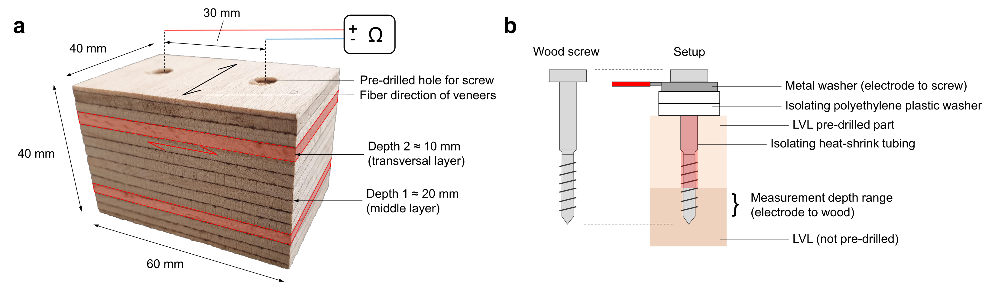
2. Materials and Methods

Two panels of “BauBuche” with dimensions of 2 m in fiber direction and 0.5 m in transversal direction were obtained from the manufacturer Pollmeier Massivholz GmbH and Co. KG at an initial MC of 6% (±2%). Each panel is composed of 14, 3 mm thick veneer layers made out of European beech (Fagus sylvatica), where the outer layers are planed by the manufacturer such that each panel had a thickness of 40 mm. The veneer layers are laminated together such that the two outer layers are glued with a melamine-formaldehyde adhesive, and the inner layers with a phenol-formaldehyde adhesive. The “BauBuche Q” panel had two transversal (cross-laminated) layers at the fourth an tenth layers, while the “BauBuche S” panel had all layers oriented in the same direction. Of each panel, 80 samples of dimensions 60 mm × 40 mm × 40 mm were cut out as shown in Figure 1a. The 80 samples of each series were divided into four subcategories of 20 samples each, and placed in four different climatic chambers with 35% RH (20 ${}^{\circ }$C), 50% RH (23 ${}^{\circ }$C), 65% RH (20 ${}^{\circ }$C), and 85% RH (20 ${}^{\circ }$C). The samples were left in the chambers for 30 days until they fulfilled the equilibrium criterion of <0.1% mass-change in 24 h. The mass-change was determined using a Mettler Toledo PR8002 scale with a precision of ±0.01 g.

The resistance measurements were carried out by a Gigamodul device from Scanntronik Mugrauer GmbH with a measurement range of 10 K$\mathsf{\Omega }$ to 100 G$\mathsf{\Omega }$. The electrodes were standard wood screws (austenitic stainless steel) of 5 mm diameter screwed into pre-drilled holes 30 mm apart as shown in Figure 1a. The holes were drilled and the electrodes were inserted after the conditioning of the samples. The detailed setup of the electrodes is depicted in Figure 1b. The resistance was measured for half of the samples per product and per climate at a depth of 20 mm (depth 1), and for the other half at a depth of 10 mm (depth 2), hitting the transverse layer in the case of “BauBuche Q”. However, since the electrode length was approximately 5 mm, glue lines were incorporated in the measurement depth range. The resistance values were determined after a 10 min stabilization time of the current through the electrodes. The electrodes were then removed and each sample was weighted. The samples were then placed in an oven at 103 ${}^{\circ }$C (±2 ${}^{\circ }$C) for 7 days until they fulfilled the equilibrium criterion of <0.1% mass-change in 24 h. The reference MC of each sample was then determined by the gravimetric method as $\mathrm{MC}=(m-m_{dry}){(m_{dry})}^{-1}$, where m is the (wet) mass after the resistance measurement and $m_{dry}$ is the dry sample mass after oven-drying. The dry density was calculated for each sample as the dry mass divided by the dry sample volume, where the estimated volume of the drilled holes was subtracted.

3. Results and Discussion

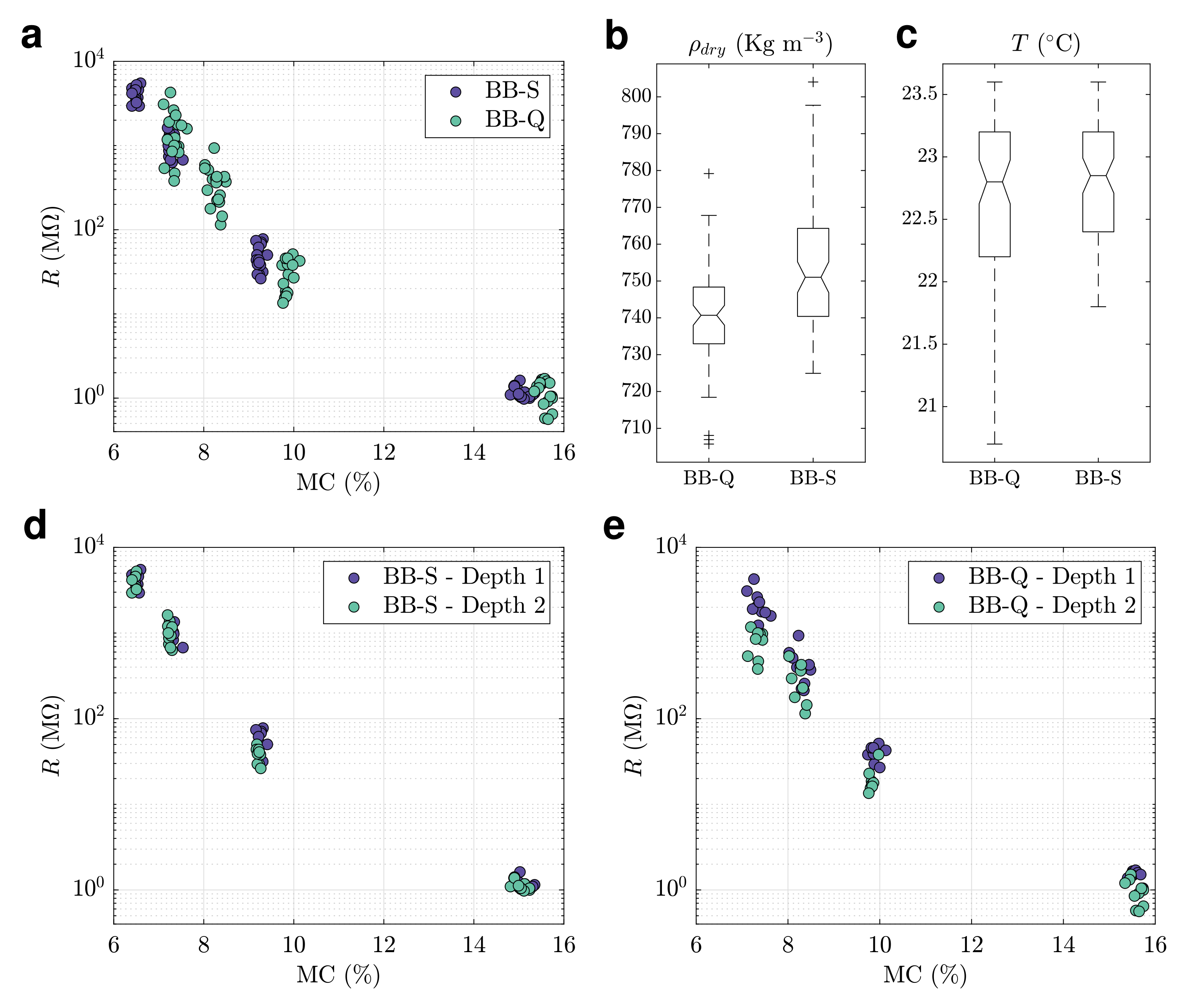
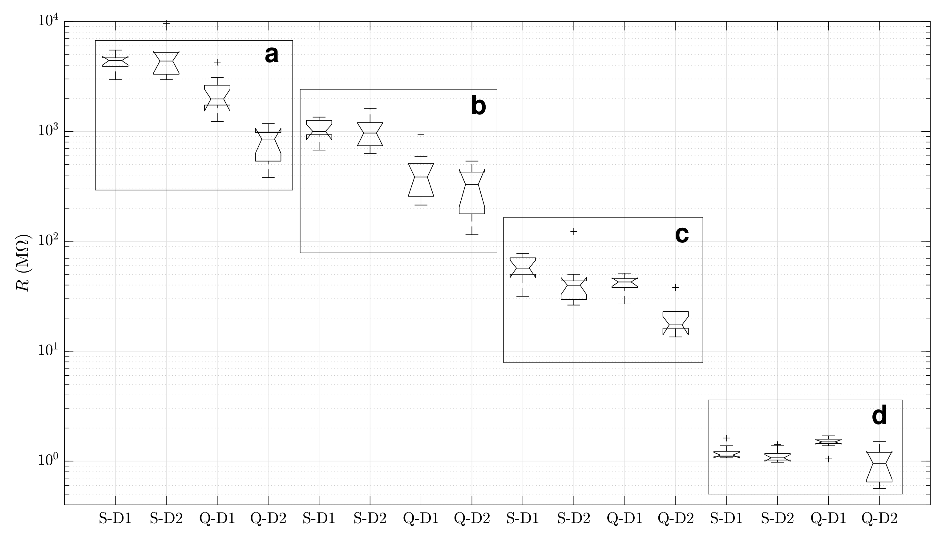
3.1. Data

Figure 2a shows the measured electrical resistance R versus the gravimetrically determined MC for the data sets “BauBuche S” (BB-S) and “BauBuche Q” (BB-Q). The data can be found in tabular form in

Table A1. Data from sample set equilibrated in 35% RH and 20 ${}^{\circ }$C climate. Type “S” represents “BauBuche S” samples, “Q” represents “BauBuche Q” samples, “D1” refers to measurement depth 1, and “D2” refers to measurement depth 2.Values marked with * designate outliers not considered in the analysis of this study. Resistance measurement values (V, unitless) are given in terms of $V=10{log}_{10}R$, so that $R={10}^{V/10}$ in units of $\mathsf{\Omega }$.

Type	$10{log}_{10}\mathit{R}$ (-)	T (${}^{\circ }$C)	MC (%)	${\mathit{\rho }}_{\mathit{dry}}$ (Kg m${}^{-3}$)	Type	$10{log}_{10}\mathit{R}$ (-)	T (${}^{\circ }$C)	MC (%)	${\mathit{\rho }}_{\mathit{dry}}$ (Kg m${}^{-3}$)
S-D1	96.30	22.60	6.47	746.70	Q-D1	93.10	22.80	7.33	749.05
S-D1	96.50	22.60	6.53	771.88	Q-D1	94.20	22.80	7.33	735.44
S-D1	96.40	22.60	6.51	732.44	Q-D1	92.00	22.80	7.63	733.62
S-D1	95.70	22.60	6.53	729.98	Q-D1	92.50	22.80	7.42	726.12
S-D1	96.70	22.60	6.51	732.33	Q-D1	92.80	23.10	7.23	736.73
S-D1	97.40	22.60	6.60	763.74	Q-D1	96.30	23.10	7.26	741.12
S-D1	94.70	22.60	6.56	737.91	Q-D1	94.90	23.10	7.11	758.59
S-D1	96.60	22.60	6.55	754.73	Q-D1	90.90	23.10	7.35	740.27
S-D1	95.90	21.80	6.48	756.34	Q-D1	93.60	23.10	7.38	755.38
S-D1	96.80	21.80	6.40	747.98	Q-D1	92.40	23.10	7.50	706.93
S-D2	96.90	21.80	6.49	752.57	Q-D2	86.70	23.10	7.35	708.08
S-D2	95.40	21.80	6.50	765.38	Q-D2	89.30	23.10	7.40	749.58
S-D2	97.20	21.80	6.51	762.71	Q-D2	90.70	22.90	7.19	749.26
S-D2	99.80 *	21.80	6.47	745.96	Q-D2	89.90	22.90	7.44	739.87
S-D2	96.60	21.80	6.48	757.16	Q-D2	89.90	22.90	7.39	745.21
S-D2	95.20	21.80	6.49	728.24	Q-D2	85.80	22.90	7.34	745.53
S-D2	108.10 *	22.80	6.42	741.80	Q-D2	89.20	22.70	7.44	731.13
S-D2	94.70	22.80	6.40	756.41	Q-D2	87.30	22.70	7.12	754.81
S-D2	96.20	22.80	6.41	779.57	Q-D2	90.00	22.70	7.34	752.68
S-D2	95.10	22.80	6.51	777.43	Q-D2	89.30	22.70	7.30	735.61

–

Table A4. Data from sample set equilibrated in 85% RH and 20 ${}^{\circ }$C climate.

Type	$10{log}_{10}\mathit{R}$ (-)	T (${}^{\circ }$C)	MC (%)	${\mathit{\rho }}_{\mathit{dry}}$ (Kg m${}^{-3}$)	Type	$10{log}_{10}\mathit{R}$ (-)	T (${}^{\circ }$C)	MC (%)	${\mathit{\rho }}_{\mathit{dry}}$ (Kg m${}^{-3}$)
S-D1	60.70	22.40	15.13	767.06	Q-D1	60.20	23.60	15.73	743.91
S-D1	60.30	22.40	15.18	746.48	Q-D1	62.20	23.60	15.51	730.51
S-D1	62.10	22.40	15.02	743.37	Q-D1	62.00	23.60	15.50	735.01
S-D1	60.50	22.40	15.06	760.20	Q-D1	62.30	23.60	15.57	739.84
S-D1	60.30	22.40	15.00	783.78	Q-D1	62.00	22.20	15.62	741.77
S-D1	60.40	22.40	15.08	727.62	Q-D1	61.70	22.20	15.51	725.58
S-D1	60.60	22.40	15.35	753.45	Q-D1	61.60	22.20	15.45	750.45
S-D1	60.90	22.40	15.00	756.77	Q-D1	61.80	22.20	15.68	719.58
S-D1	60.40	23.40	15.31	749.91	Q-D1	61.60	22.20	15.47	742.52
S-D1	61.40	23.40	14.89	739.84	Q-D1	61.40	22.20	15.40	742.52
S-D2	60.70	23.40	15.13	750.54	Q-D2	61.80	22.20	15.47	739.45
S-D2	60.10	23.40	15.04	769.54	Q-D2	60.00	22.20	15.74	734.86
S-D2	60.00	23.40	15.24	744.36	Q-D2	57.60	23.40	15.58	746.60
S-D2	60.20	23.40	15.24	740.94	Q-D2	59.60	23.40	15.64	721.10
S-D2	61.50	23.40	14.90	776.15	Q-D2	60.20	23.40	15.70	718.43
S-D2	59.90	23.40	15.11	773.81	Q-D2	59.30	23.40	15.55	723.98
S-D2	60.40	23.60	14.81	754.17	Q-D2	58.10	23.40	15.74	720.45
S-D2	60.20	23.60	15.05	729.63	Q-D2	57.50	23.40	15.65	705.73
S-D2	61.40	23.60	14.90	746.17	Q-D2	61.20	23.40	15.44	742.86
S-D2	60.50	23.60	14.99	767.19	Q-D2	60.80	23.40	15.34	757.37

in the appendix. It is apparent, that BB-S and BB-Q reached different equilibrium MCs while stored in the same climate conditions. Next to effects that may have been caused by initial MCs of the panels or different swelling behavior of BB-S and BB-Q, this difference could also be due to the difference in dry density shown in Figure 2b. The mean value of the oven-dry density was 752.89 Kg m${}^{-3}$ for the set BB-S, and 739.80 Kg m${}^{-3}$ for the set BB-Q, with standard deviations of 16.58 Kg m${}^{-3}$ and 12.64 Kg m${}^{-3}$ respectively. However, it is known that the wood density does not influence the electrical resistance [5,24]. Therefore, different calibrations for resistance between BB-S and BB-Q would not be required based only on their difference in density.

The mean value of the temperature recorded during resistance measurements of the 160 samples was 22.68 ${}^{\circ }$C with a standard deviation of 0.74 ${}^{\circ }$C. Since there is no apparent difference in temperature between BB-S and BB-Q measurements, as illustrated in Figure 2c, the influence of temperature can be neglected for the calibration process. However, an apparent difference in resistance at the different measurement depths 1 (20 mm, middle layer) and 2 (10 mm, transversal layer for BB-Q) can be observed for the sample sets BB-Q (Figure 2e), while this is not the case for BB-S (Figure 2d). The differences of resistance in depths 1 and 2 of the BB-Q samples were found to be significant for the sample sets equilibrated at the 35%, 65%, and 85% RH climates (see Figure A1 in the Appendix A). Lower resistances were measured at the depth of the transversal layer (parallel to wood fiber direction), meaning that the electric conductance is indeed influenced if the electrode penetrates the transversal layer in “BauBuche Q”. Based on this, it can be concluded that three different calibrations are necessary: For BB-S, for BB-Q at depth 1, and for BB-Q at depth 2.

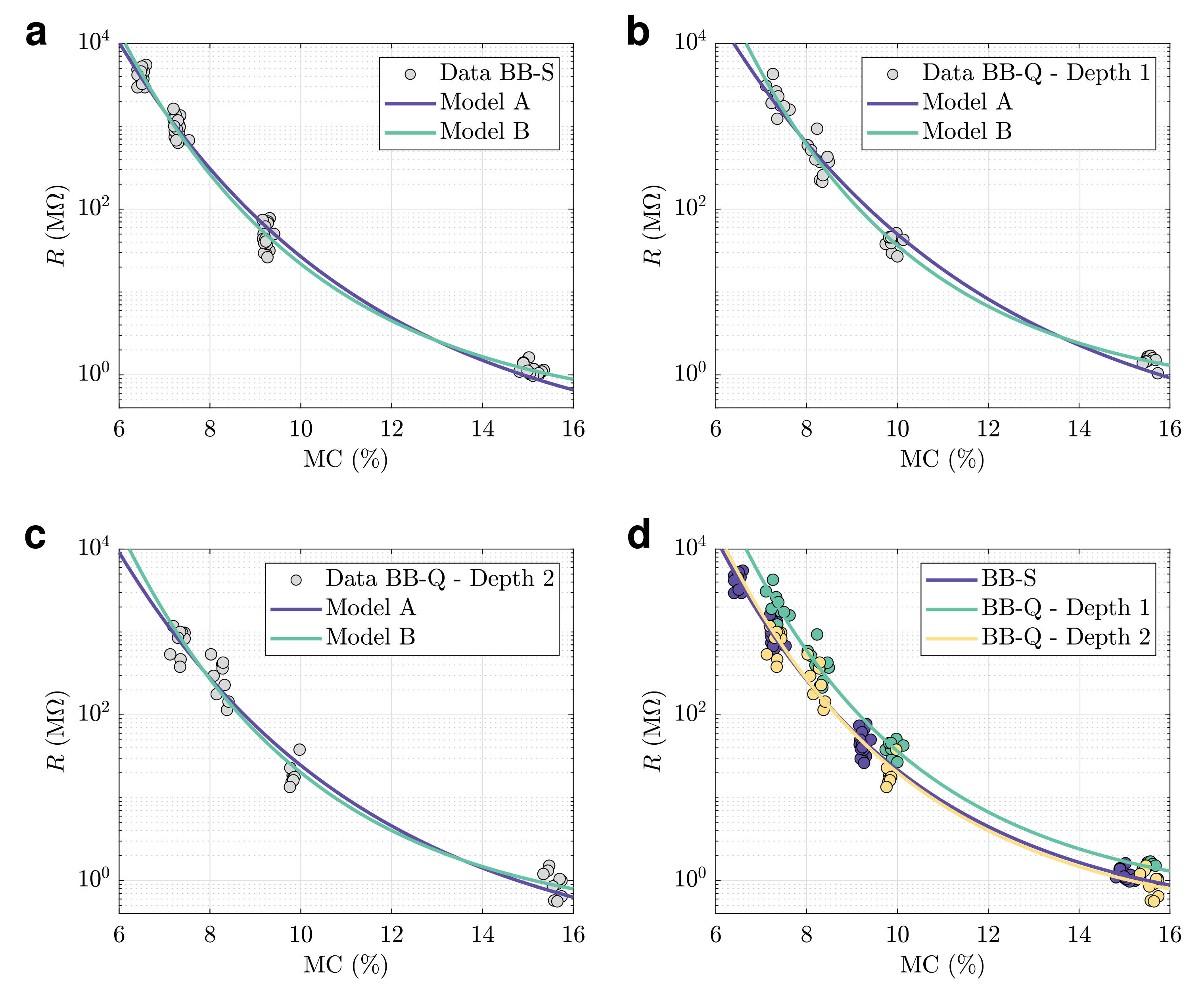
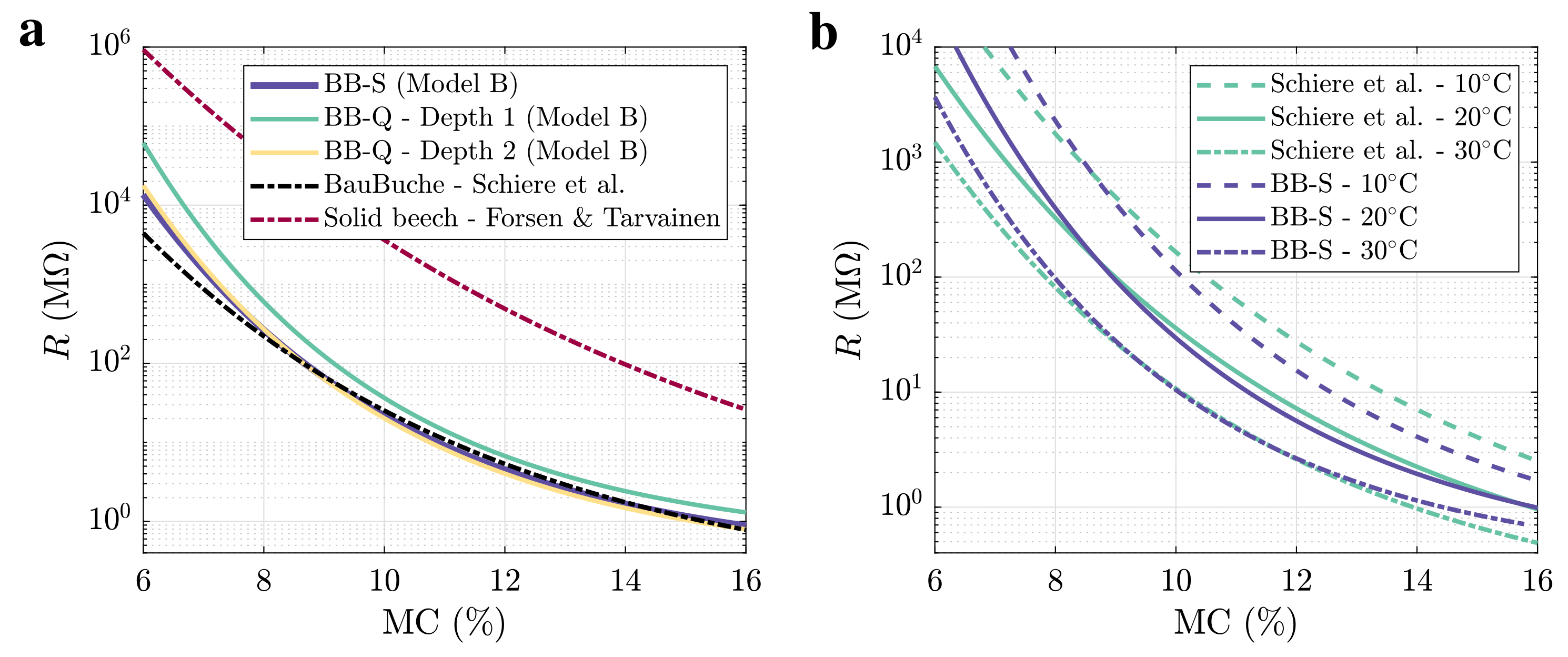
3.2. Calibration Models

Calibration models for resistance to wood MC generally take the form of a double logarithmic expression of the resistance R versus a linear function of the MC [5,25,26]. However, there is no consensus on whether a model shall use two or three fitting parameters, and whether the natural or a base-10 logarithm should be used. In this study, two of the more common calibration models are used:

$${log}_{10}({log}_{10}(R)+1)=A_1·\mathrm{MC}+A_2,$$

(1)

$${log}_{10}({log}_{10}(R)+B_3)=B_1·\mathrm{MC}+B_2.$$

(2)

Hereafter, these two models are denoted model A and model B. The fitting parameters $A_1,A_2$ for model A and $B_1,B_2,B_3$ for model B were determined by a linear regression analysis to the data shown in Figure 2. The fitted parameters are shown in

Table 1. Calibration model parameters for model A and B as determined by regression analysis for the sample sets “BauBuche S” (BB-S), “BauBuche Q” at depth of the middle layer (BB-Q-Depth 1), and “BauBuche Q” at depth of the transversal layer (BB-Q-Depth 2).

	Model A			Model B
	${log}_{\mathbf{10}}\mathit{R}={\mathbf{10}}^{{\mathit{A}}_{\mathbf{1}}·\mathbf{MC}+{\mathit{A}}_{\mathbf{2}}}-\mathbf{1}$			${log}_{\mathbf{10}}\mathit{R}={\mathbf{10}}^{{\mathit{B}}_{\mathbf{1}}·\mathbf{MC}+{\mathit{B}}_{\mathbf{2}}}-{\mathit{B}}_{\mathbf{3}}$
	${\mathit{A}}_{\mathbf{1}}$	${\mathit{A}}_{\mathbf{2}}$	adj.R${}^{\mathbf{2}}$	${\mathit{B}}_{\mathbf{1}}$	${\mathit{B}}_{\mathbf{2}}$	${\mathit{B}}_{\mathbf{3}}$	adj.R${}^{\mathbf{2}}$
BB-S	−0.07868	1.172	0.9910	−0.0996	1.266	0.5248	0.9937
BB-Q-Depth 1	−0.07441	1.175	0.9822	−0.1093	1.362	0.2956	0.9896
BB-Q-Depth 2	−0.07924	1.171	0.9681	−0.1036	1.302	0.5409	0.9710

and the calibration curves are shown in Figure 3a–d for the three separate data series of “BauBuche” samples. The goodness-of-fit was evaluated by adjusted R${}^2$ values in order to be able to compare between the two models with different fitting parameters (Table 1). It can be seen that model B appeared to fit the data better for all three separate series, justifying the use of an additional parameter. Therefore, if not for the simplicity of a two-parameter model, the authors recommend using model B for the calibration of R to MC for “BauBuche”. The three calibrations of this study appeared to agree very well to a calibration for “BauBuche S” from Schiere et al. [23], as shown in Figure 4a, and the beech LVL calibrations indeed differed from a calibration for solid European beech wood [26].

3.3. Temperature Correction

The electrical resistance in wood decreased as the temperature increased, and vice-versa. It is known that the influence of temperature on resistance-calibrated wood MC is approximately linear [25]. The absolute error in MC was about 0.1–0.15% per each ${}^{\circ }$C of deviation from the calibration temperature [26]. Therefore, and for simplicity, an approach of linear correction of MC was chosen here. The following temperature correction equation is suggested in Skaar [5], based on James [24,27]:

$$\mathrm{MC}(R,T)=\frac{\mathrm{MC}(R)-0.027(T-22.68)}{0.0085(T-22.68)+1},$$

(3)

where $\mathrm{MC}(R,T)$ (%) is the corrected MC at temperature T (${}^{\circ }$C) of the resistance measurement, $\mathrm{MC}(R)$ (%) is the MC as calculated by the calibration models presented above, and 22.68 ${}^{\circ }$C is the value of the calibration temperature of $\mathrm{MC}(R)$. Even though the theoretical value of the calibration temperature of the data should be 21 ${}^{\circ }$C according to Skaar [5], it is assumed that Equation (3) can be used without noticeable loss in precision. Furthermore, Equation (3) was verified for both calibration models A and B against a more complex correction model suggested in Pfaff and Garrahan [28], and the corrections were found to match with negligible differences. In theory, a more accurate and data-based temperature correction of the calibration curves for beech LVL would be possible by collecting further data at different temperatures. In fact, a detailed study conducted by Boardman et al. [29] on oriented strand board showed that the temperature dependence is more complex than assumed previously. This might also be the case for further engineered wood products such as LVL. For beech LVL, a data-based temperature-corrected calibration was made in Schiere et al. [23]; however, the calibration is based on data points collected only at 10 ${}^{\circ }$C and 20 ${}^{\circ }$C. Furthermore, Figure 4b shows that a data-based temperature correction did not add an apparent benefit in terms of precision in the case of beech LVL. It can be seen that the corrections of BB-S using Equation (3) coincided closely with the data-based corrections from Schiere et al. [23] for 10 ${}^{\circ }$C and 20 ${}^{\circ }$C. In the case of 30 ${}^{\circ }$C the agreement was slightly less.

3.4. Limitations

The validity of the calibration curves derived in this study is exclusive to the type and setup of electrodes as shown in Figure 1. The type and size of the electrodes, but also of the specimens can potentially influence the measurements [30]. A limitation might also apply to the choice of the three different calibration curves, as e.g., all 80 samples for BB-S originated from the same panel provided by the manufacturer. Therefore, it cannot be suggested with certainty that a different calibration for the two different measurement depths will be necessary for all BB-Q panels in general. However, the three calibrations of “BauBuche” in this study are close to one another in relation to solid beech, and they display a nearly perfect agreement with data from Schiere et al. [23] obtained with different types of electrodes and different panels. Due to the assumption on temperature correction, the range of application should be limited to heated indoor conditions where the MC does not vary in an extreme manner. The calibrations were conducted for a range of application of 6% < MC < 16% based on data collected at approximately 6% < MC < 11% and 14.5% < MC < 16%, with a missing data range between 11% and 14.5%.

A recent study by Fredriksson et al. [31] showed that moisture gradients in wood can have an impact on resistance measurements. In real timber structures, moisture gradients usually predominate over steady-state moisture conditions. Consequently, nondestructive MC-monitoring by resistance measurements, at least for electrode depths close to the surface, will not be able to achieve a certain targeted precision regardless of the calibration model. Accordingly, the validity and limitations of calibration models should be put in the general perspective of desired accuracy in monitoring campaigns. This applies in particular to structural components made from “BauBuche S” and “BauBuche Q” panels that are only 40 mm thick.

The suggested calibration for beech LVL shows a clear difference to native beech wood (Figure 4a). However, this difference can not be explained in the present study. It is unclear whether the glue lines or the altered physical properties of the wood material itself influenced the measurements. James [24] recommends using specialized veneer electrodes suitable for measuring resistance in material layers down to 3 mm thickness. This approach, although more tedious and impractical for long-term monitoring studies of MC, would rule out the effect of glue lines, allowing to capture the true impact the specific LVL production treatment had on the material. This impact is believed to be strong as Schiere et al. [23] showed, based on measurements perpendicular to glue lines (glue lines in series), that the resistance in beech LVL seems not very much influenced by the latter, but indeed seems to be majorly a consequence of altered physical properties. A recent study by Engehausen et al. [19] showed that the veneer density is altered in the regions around the adhesive interface either by densification of the wood material or by penetration of the adhesive, but that further research is needed in order to clarify the exact cause and effects on physical properties.

4. Conclusions

For the beech LVL panel products “BauBuche”, three different calibrations for resistance to MC are necessary: For “BauBuche S”, for “Baubuche Q” when the electrodes are in the middle layer, and for “BauBuche Q” when the electrodes are in the transversal layer. In all three cases, double-logarithmic calibration models with three parameters achieve a better fit based on adjusted R${}^2$ values than models with two parameters. However, measurements of MC by electrical resistance is still deemed a non-trivial task in the case of beech LVL, and some limitations specific to this study, such as electrode setup, moisture range, or representativity of the results must be considered in practise.

References

1. Dietsch, P.; Franke, S.; Franke, B.; Gamper, A.; Winter, S. Methods to determine wood moisture content and their applicability in monitoring concepts. J. Civ. Struct. Health Monit. 2015, 5, 115–127. [Google Scholar] [CrossRef]
2. Palma, P.; Steiger, R. Structural health monitoring of timber structures–Review of available methods and case studies. Constr. Build. Mater. 2020, 248, 118528. [Google Scholar] [CrossRef]
3. Llana, D.F.; Íñiguez González, G.; Esteban, M.; Hermoso, E.; Arriaga, F. Timber moisture content adjustment factors for nondestructive testing (NDT): Acoustic, vibration and probing techniques. Holzforschung 2020, 74, 817–827. [Google Scholar] [CrossRef]
4. Stamm, A.J. The Electrical Resistance of Wood as aMeasure of Its Moisture Content. Ind. Eng. Chem. 1927, 19, 1021–1025. [Google Scholar] [CrossRef]
5. Skaar, C. Wood-Water Relations; Springer Series in Wood Science; Springer: Berlin/Heidelberg, Germany, 1988. [Google Scholar]
6. Hassan, J.; Eisele, M. BauBuche-the sustainable high-performance material. Bautechnik 2015, 92, 40–45. [Google Scholar] [CrossRef]
7. Kobel, P.; Steiger, R.; Frangi, A. Experimental Analysis on the Structural Behaviour of Connections with LVL Made of Beech Wood. In Materials and Joints in Timber Structures: Recent Developments of Technology; Aicher, S., Reinhardt, H.W., Garrecht, H., Eds.; RILEM Bookseries: Dordrecht, The Netherlands, 2014; Volume 9, pp. 211–220. [Google Scholar] [CrossRef]
8. Enders-Comberg, M.; Frese, M.; Blaß, H.J. Buchenfurnierschichtholz für Fachwerkträger und verstärktes Brettschichtholz. Bautechnik 2015, 92, 9–17. [Google Scholar] [CrossRef]
9. Sebastian, W.M.; Mudie, J.; Cox, G.; Piazza, M.; Tomasi, R.; Giongo, I. Insight into mechanics of externally indeterminate hardwood-concrete composite beams. Constr. Build. Mater. 2016, 102, 1029–1048. [Google Scholar] [CrossRef]
10. Stepinac, M.; Rajcic, V.; Hunger, F.; van de Kuilen, J.W.G. Glued-in rods in beech laminated veneer lumber. Eur. J. Wood Wood Prod. 2016, 74, 463–466. [Google Scholar] [CrossRef]
11. Boccadoro, L.; Zweidler, S.; Steiger, R.; Frangi, A. Bending tests on timber-concrete composite members made of beech laminated veneer lumber with notched connection. Eng. Struct. 2017, 132, 14–28. [Google Scholar] [CrossRef]
12. Aicher, S.; Tapia, C. Novel internally LVL-reinforced glued laminated timber beams with large holes. Constr. Build. Mater. 2018, 169, 662–677. [Google Scholar] [CrossRef]
13. Myslicki, S.; Vallee, T.; Bletz-Muehldorfer, O.; Diehl, F.; Lavarec, L.C.; Creac’Hcadec, R. Fracture mechanics based joint capacity prediction of glued-in rods with beech laminated veneer lumber. J. Adhes. 2019, 95, 405–424. [Google Scholar] [CrossRef]
14. Steige, Y.; Frese, M. Study on a newly developed diagonal connection for hybrid timber trusses made of spruce glulam and beech laminated veneer lumber. Wood Mater. Sci. Eng. 2019, 14, 280–290. [Google Scholar] [CrossRef]
15. Benthien, J.T.; Riegler, M.; Engehausen, N.; Nopens, M. Specific Dimensional Change Behavior of Laminated Beech Veneer Lumber (BauBuche) in Terms of Moisture Absorption and Desorption. Fibers 2020, 8, 47. [Google Scholar] [CrossRef]
16. Pot, G.; Denaud, L.E.; Collet, R. Numerical study of the influence of veneer lathe checks on the elastic mechanical properties of laminated veneer lumber (LVL) made of beech. Holzforschung 2015, 69, 337–345. [Google Scholar] [CrossRef]
17. Viguier, J.; Marcon, B.; Girardon, S.; Denaud, L. Effect of Forestry Management and Veneer Defects Identified by X-ray Analysis on Mechanical Properties of Laminated Veneer Lumber Beams Made of Beech. Bioresources 2017, 12, 6122–6133. [Google Scholar] [CrossRef] [Green Version]
18. Fleckenstein, M.; Biziks, V.; Mai, C.; Militz, H. Modification of beech veneers with lignin phenol formaldehyde resins in the production of laminated veneer lumber (LVL). Eur. J. Wood Wood Prod. 2018, 76, 843–851. [Google Scholar] [CrossRef]
19. Engehausen, N.; Benthien, J.T.; Nopens, M.; Ressel, J.B. Density Profile Analysis of Laminated Beech Veneer Lumber (BauBuche). Fibers 2021, 9, 31. [Google Scholar] [CrossRef]
20. Leyder, C. Monitoring-Based Performance Assessment of an Innovative Timber-Hybrid Building. Ph.D. Thesis, ETH Zurich, Zurich, Switzerland, 2018. [Google Scholar] [CrossRef]
21. Jockwer, R.; Grönquist, P.; Frangi, A. Long-term deformation behaviour of timber columns: Monitoring of a tall timber building in Switzerland. Eng. Struct. 2021, 234, 111855. [Google Scholar] [CrossRef]
22. Franke, B.; Franke, S.; Schiere, M.; Müller, A. Quality Assurance of Timber Structures; Technical Report Research Report Nr. 77FE-008098-V01; Bern University of Applied Sciences, Institute for Timber Constructions, Structures and Architecture: Biel, Switzerland, 2019. [Google Scholar]
23. Schiere, M.; Franke, B.; Franke, S.; Müller, A. Calibration and Comparison of Two Moisture Content Measurement Methods for In Situ Monitoring of Beech Laminated Veneer Lumber. 2021; Manuscript Submitted for Publication. [Google Scholar]
24. James, W.L. Electric Moisture Meters for Wood; Technical Report Gen. Tech. Rep. FPL-GTR-6; U.S. Department of Agriculture, Forest Service, Forest Products Laboratory: Madison, WI, USA, 1975. [Google Scholar]
25. Keylwerth, R.; Noack, D. Über den Einfluß höherer Temperaturen auf die elektrische Holzfeuchtigkeits-messung nach dem Widerstandsprinzip. Holz Als Roh-Und Werkst. 1956, 14, 162–172. [Google Scholar] [CrossRef]
26. Forsén, H.; Tarvainen, V. Accuracy and Functionality of Hand Held Wood Moisture Content Meters; Technical Report Espoo 2000; Technical Research Centre of Finland, VTT Publications 420: Espoo, Finland, 2000. [Google Scholar]
27. James, W.L. Dielectric Properties of Wood and Hardboard. Variation with Temperature, Frequency, Moisture Content, and Grain Orientation; Technical Report Gen. Res. Pap. FPL-245; U.S. Department of Agriculture, Forest Service, Forest Products Laboratory: Madison, WI, USA, 1975. [Google Scholar]
28. Pfaff, F.; Garrahan, P. New temperature correction factors for the portable resistance-type moisture meter. For. Prod. J. 1985, 36, 28–30. [Google Scholar]
29. Boardman, C.; Glass, S.V.; Lebow, P.K. Simple and accurate temperature correction for moisture pin calibrations in oriented strand board. Build. Environ. 2017, 112, 250–260. [Google Scholar] [CrossRef] [Green Version]
30. Fredriksson, M.; Claesson, J.; Wadsö, L. The Influence of Specimen Size and Distance to a Surface on Resistive Moisture Content Measurements in Wood. Math. Probl. Eng. 2015. [Google Scholar] [CrossRef] [Green Version]
31. Fredriksson, M.; Thybring, E.E.; Zelinka, S.L. Artifacts in electrical measurements on wood caused by non-uniform moisture distributions. Holzforschung 2020. [Google Scholar] [CrossRef]
Figure 1. (a) Picture of samples with dimensions, measurement depths 1 and 2, and drilled holes for screws (electrodes). Shown is a picture of a “BauBuche Q” sample (transversal layer highlighted in red). (b) Setup of electrode during measurements (assembly on screw).
Forests 12 00635 g001
Figure 2. Measured electrical resistance (R) vs. gravimetric moisture content (MC): (a) Samples of “BauBuche S” (BB-S) compared to samples of “BauBuche Q” (BB-Q). (b) Oven-dry density of samples ( ρ d r y ), notches in boxplots represent 95% confidence interval of the median. (c) Temperature (T) during measurement of R (d) BB-S samples sorted by two measurement depths 1 (20 mm) and 2 (10 mm). (e) BB-Q samples sorted by two measurement depths 1 (20 mm) and 2 (10 mm, depth of transversal layer).
Forests 12 00635 g002
Figure 3. Fitting of calibration models A and B: (a) models fitted to data of “BauBuche S” (BB-S). (b) Models fitted to data of “BauBuche Q” (BB-Q) at depth 1 (depth of middle layer, 20 mm). (c) Models fitted to data of “BauBuche Q” (BB-Q) at depth 2 (depth transversal layer, 10 mm, electrical current parallel to wood fiber). (d) Fitted models B compared with each-other and with data.
Forests 12 00635 g003
Figure 4. (a) Comparison of calibration models B at 22.68 C with Literature calibrations for “BauBuche S” from Schiere et al. [23], and for solid central European beech wood from Forsén and Tarvainen [26] with A 1 = 0.046 and A 2 = 1.119 using model A. (b) Temperature corrections for 10 C, 20 C, and 30 C for BB-S using model B and Equation (3) compared to data-based temperature corrections for “BauBuche S” from Schiere et al. [23].
Forests 12 00635 g004