
Assessing Forest Structural and Topographic Effects on Habitat Productivity for the Endangered Apennine Brown Bear


1
Department of Biology and Biotechnology, University of Rome, P.le Aldo Moro 5, 00185 Rome, Italy
2
Department of Statistical Sciences, University of Rome, P.le Aldo Moro 5, 00185 Rome, Italy
*
Author to whom correspondence should be addressed.
Forests 2021, 12(7), 916; https://0-doi-org.brum.beds.ac.uk/10.3390/f12070916
Submission received: 15 June 2021
/
Revised: 10 July 2021
/
Accepted: 12 July 2021
/
Published: 14 July 2021
(This article belongs to the Special Issue Conservation of Threatened Forest-Dwelling Species and Intact Forest Ecosystems)
Abstract
:Any forest management potentially affects the availability and quality of resources for forest-dwelling wildlife populations, including endangered species. One such species is the Apennine brown bear, a small and unique population living in the central Apennines of Italy. The conservation of this relict bear population is hampered by the lack of knowledge of the fine-scale relationships between productivity of key foods and forest structure, as this prevents the design and implementation of effective forest management plans. To address this issue, we sampled the main structural stand attributes within the bear’s range and used multivariate generalized linear mixed models in a Bayesian framework to relate forest structural attributes to proxies of productivity of key bear foods. We found that hard mast was positively associated with both forest typology and high forest system, but negatively related to both the time elapsed since the last forest utilization and the amount of deadwood. The availability of soft-mast producing species was positively related to past forestry practices but negatively associated with steep slopes historically managed with high tree densities and a low silvicultural disturbance. Our findings also suggest that herb cover was negatively affected by terrain steepness and basal area, while herb productivity was positively affected by northern and southern exposure. Additionally, richness of forest ants was associated with forests characterized by low volume and high density. Our findings confirm that the productivity of natural bear foods is strongly affected by forest structural and topographical characteristics and are relevant as preliminary information for forest management practices to support the long-term conservation of Apennine bears.
1. Introduction
Forestry has historically focused on maximizing the wood production of economically desirable tree species. Recently, increasing environmental concern and a growing body of scientific literature has led to a greater awareness of forests as ecological systems with inherent value that needs careful consideration. Forests provide a wide range of important ecosystem services, e.g., climate regulation, carbon sequestration and storage, water regulation, biological control, and nutrient cycling [1]. Indeed, forests also support biodiversity and provide habitats for wildlife species; the term ‘habitat’ indicates the set of resources and conditions necessary to support an animal population through space and time [2]. Therefore, forest management can unconsciously or intentionally alter resources for forest-dwelling wildlife species by interfering with successional stages and altering composition of species, vertical stratification of trees, and age structure [3]. Forestry practices may additionally alter microscale habitat conditions such as temperature, light, moisture, soil, and litter status [4]. It follows that any forest management practice, including an absence of direct interventions (e.g., in protected areas), has potential short- and long-term effects on the availability, distribution, and quality of habitats resources for forest-dwelling wildlife species [5]. Because habitat requirements vary deeply among wildlife species, and in accordance with the sequence of seral stages, timber harvest can improve habitat quality for some species while at the same time deteriorating habitat suitability for others. Accordingly, large-scale logging in mature stands draws back the vegetation community from late to early successional stages, benefitting wildlife species more adapted to the early successional stages [6].
Several studies have investigated the effects of forest management on habitat suitability of forest-dwelling wildlife (and biodiversity in general), including some meta-analyses. According to these investigations, the type and extent of the effects of forestry on wildlife habitat vary deeply depending, above all, on species and taxonomic group [7,8,9], the forest management system [9,10], the extent of logging [11], the time since logging [5,12,13], and the overall landscape matrix [13,14], revealing a mix of complementary and compound relationships. Silviculture is, therefore, a powerful tool to achieve wildlife management aims. Creating and manipulating disturbance regimes of forests can enhance the spatial and temporal arrangement of key forest characteristics used or selected by a given wildlife species and can therefore improve quality of the species’ habitat [15]. This is especially true for the small or threatened wildlife populations in greatest need of active management interventions, and of which the long-term effective conservation rests on structural improvements of their habitat at the landscape scale [5].
The Apennine brown bear (Ursus arctos marsicanus) survives in a small and isolated population consisting of about 50 individuals [16] confined to the Abruzzo, Lazio, and Molise National Park (PNALM) and its surrounding region in central Italy. This bear population faces a severe risk of extinction due to small size and reduced genetic variability [17,18]. In addition to mitigation of human-caused mortality and disturbance, habitat management to ensure long-term productivity of the forest ecosystem has been advocated to facilitate expansion of the species’ range [19,20,21]. In fact, no significant expansion of the bear range has been recently observed, despite the availability of suitable habitat at the landscape scale and a number of protected areas therein [20,22,23]. This is probably due to high levels of human-caused mortality [23], a relatively low reproductive performance [24], and the likely contribution of stochasticity [18,25]. Based on projections of habitat suitability at the landscape scale, the conditions and connectivity of high-quality habitat patches in the central Apennines have been deemed adequate to support a viable population of Apennine bears [20]. However, available estimates of habitat and landscape suitability did not take into account forest management practices and their effects on forest structure and productivity. Indeed, a more in-depth knowledge of how forest structure and management practices relate to habitat suitability and food productivity for Apennine bears is therefore fundamental to inform forest management [26].
The availability and accessibility of nutritionally adequate food resources are critical drivers of high-quality bear habitat [27,28,29]. Similarly, to other south-European bear populations [30], Apennine bears have a prevalently vegetarian diet and, even though they consume a wide variety of foods, plant-based items tend to be consumed more frequently throughout the year [26]. In spring and early summer, herbaceous vegetation represents 19–31.7% of their digestible energy, complemented by wild ungulates and a significant contribution of ants, while berries contribute 56.5% in summer, and in fall, the majority of digestible energy is represented by hard mast (66.9%) followed by fleshy fruits (26.3%) [26]. The mountain forests of the central Apennines are thought to broadly fulfil the habitat requirements for Apennine brown bears, such as food and thermal and security cover [22,23]. However, a lack of detailed data on the relationship between fine-scale forest structure and composition and food productivity prevents the planning of effective forest management to assist the conservation of Apennine bears. Nevertheless, forestry practices are known to play a critical role in affecting the availability of seasonal key foods for bears, especially during hyperphagy [31]. This is a critical period of the year for bears, as they need to swiftly accumulate fat for the wintering period. In many bear populations, the amount of fat accumulated during fall is correlated with reproductive success [32,33,34,35], as fat storage in reproducing females is an essential source of energy for cub production and lactation [36]. In particular, the availability of hard mast (i.e., beechnuts, acorns) during fall, complemented by fleshy fruits, seems to boost reproductive success in Apennine female bears [37]. Although a substantial body of research has determined how forest management can affect habitat quality for black (Ursus americanus) (e.g., [38,39,40]) and grizzly (Ursus arctos) (e.g., [13,31,41,42,43,44,45]) bears, no such information is currently available for Apennine brown bears [46]. To fill this knowledge gap, the aim of this study was to investigate the relationship between fine-scale forest structure metrics, reflecting forest structure and management practices, and indirect measures of productivity of key foods for Apennine bears. By collecting forest structural metrics during the fall, we focused on forest-related key foods consumed by bears during hyperphagia (soft and hard mast), even though we also made inferences regarding key foods consumed by bears in other seasons. Since topography is known to affect forest structure and composition [47,48] and, in turn, habitat conditions for forest-dwelling species [49], we also considered topographical features as factors potentially affecting productivity of bear key foods. We hypothesized that food availability for bears varies as a function of the structural and topographical characteristics of forests. To this end, we predicted that forest structural predictors could be identified for each food item, implying that these can be manipulated to improve the habitat productivity of bears.
2. Materials and Methods
2.1. Study Area
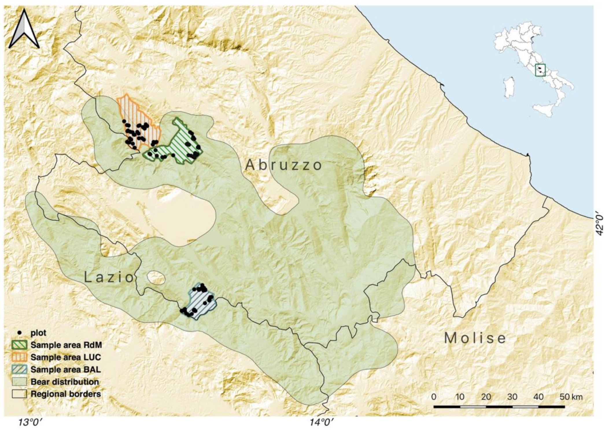
The study was conducted in the central Apennines (Figure 1) of the Abruzzo region (central Italy). In order to assess forest structure and composition in both the core and the peripheral portions of the bear range [19], we selected three sample areas: Balsorano (BAL), featuring a forested area of 4490 ha that lies within the core bear range and is partially included in the Abruzzo Lazio and Molise National Park (PNALM); Rocca di Mezzo (RdM), featuring a forested area of 5570 ha in the Sirente-Velino Regional Park, in a zone of the peripheral range where bears are permanently present even though at lower densities compared to the core range [50]; and Lucoli (LUC), featuring a forested area of 5790 ha, within the outer portion of the peripheral range and where bear occurrence is sporadic and mostly limited to erratic bears. All three sample areas have a temperate oceanic climate, which ranges to semicontinental in the inner valley [51]. Elevation ranges from 690 to 1850 m a.s.l. and orography is typically mountainous. Locally, beech forests (Fagus sylvatica) are predominant, representing on average 66% (SD = 17%) of the entire forest cover. The remaining forests are oak (Quercus spp.) and hop hornbeam (Ostrya carpinifolia) woods, with tree species composition varying with aspect and altitude [52]. Since the 1950s, forestry operations in these areas have been exclusively associated with a levy of resident populations and are managed by local administrations to meet firewood needs. According to forest management plans, the last harvest cut for commercial purposes was done in the 1970s, when forests were managed according to a shelterwood system (A. Rositi, unpublished data). More recently, more intensive harvesting systems have almost disappeared in most of the Apennines [53]. According to official estimates, from 2001 to 2015, forest production in the Abruzzo region was mainly aimed at wood fuel production (about 96% of the total) and, during the same period, the total area harvested decreased by about 95% (Istituto Nazionale di Statistica, http://dati.istat.it, accessed on 7 April 2020). As a consequence, forests in the study area are currently characterized by over-mature coppice (the ordinary rotation has been passed) or areas in the early stages of natural conversion to high forest, and high forests managed in previous decades according to a shelterwood system. Due to an inadequate implementation of the management system in the form of very heavy initial cuts and no removal cuttings [54], forests in the study area currently display an irregular structure (Table 1).
2.2. Study Design
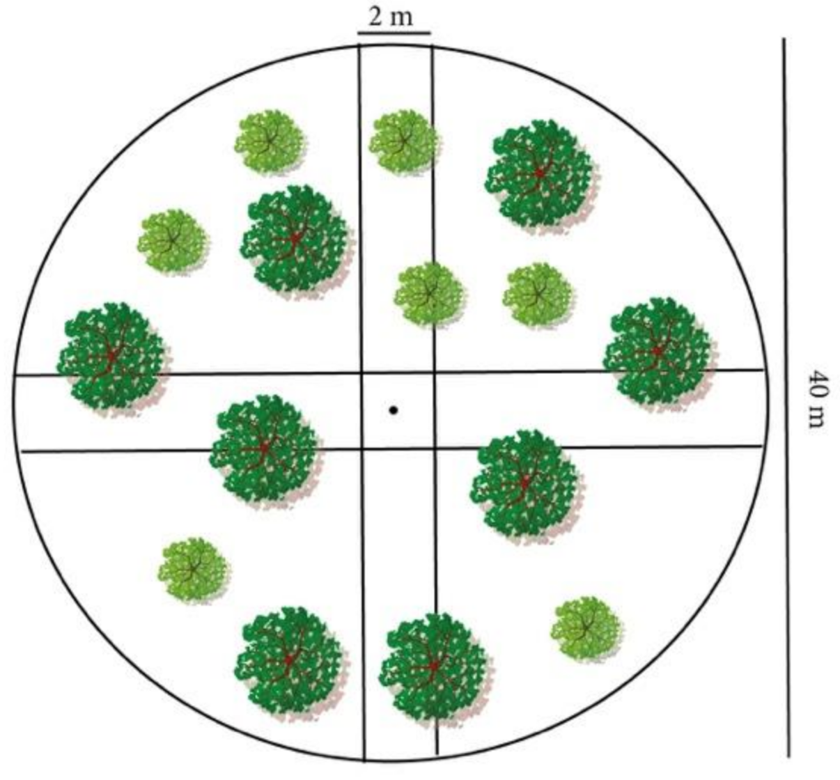
To sample forest structural metrics, we first calculated the extent of forested areas within the study area from regional maps of forest types (http://geoportale.regione.abruzzo.it/Cartanet/viewer; accessed on 7 April 2020), excluding rocky areas, scrubland, and artificial plantations (i.e., conifers), as these occurred in negligible proportions. We then defined two strata based on the prevailing forest system (i.e., coppice vs. high forest) and applied stratified random sampling by randomly selecting the coordinates of each plot (20 m radius) within each stratum. Using a total of 90 plots across the entire study area, we allocated the plots in each sample area proportionally to its size, whereas the number of plots in each stratum was proportional to the coefficient of variation of the basal area of trees, the latter being obtained from preliminary sampling in each stratum. To avoid edge effects on the forest structure, we located plots within forest patches excluding a 50 m inner buffer. To investigate the effect of topographic factors, we also recorded variables related to topography (i.e., aspect, altitude, slope, steepness), position of plots within the landscape (i.e., ridge top, ridge side, and valley bottom), and forest regeneration (species and type of distribution). Furthermore, we recorded soil type using physiographic classes (landforms combined with lithology), as the study area consists mainly of limestone [55]. We also registered the coordinates of the center of each plot as a proxy of territorial administrative unit. Within each plot, we placed four 20 × 2 m (Figure 2) perpendiculars transects (North–south, east–west) along which we collected data on stand structure and proxies of abundance of bear key foods (see below).
2.3. Data Collection
To investigate the relationships between forest structure and proxies of key bear foods, we recorded main structural stand attributes related to tree dimension, species composition, and deadwood [56]. Specifically, within each plot, we surveyed all living trees and measured diameters (DBH ≥ 3 cm), total heights, and height of live crown. In order to define vertical structure and number of strata, we used the Pretzsch diversity index [57] and the Latham index [58], setting the competition zone of the latter to 60% of crown [59]. We summarized species composition and diversity using the Shannon index (SH) [60], Simpson’s dominance (D) [61], Pielou Eveness index (E) [62], and S (number of tree species). We also considered the deadwood category, comprising standing deadwood, logs, snags, stumps, and lying woods with diameter ≥ 5 cm, and for each we determined species, number, size (diameter and height) and volume. We estimated the volume of standing trees ≥4 m in height and snags using double-entry volume tables [63]; for snags of <4 m, we used the Huber formula [64]. We then assigned each deadwood component to a decay class based on a visual assessment of morphological characteristics using a five-class system [65] customized according to the BIOSOL project [66]. We used the number of decay classes as an index of forestry operations—i.e., the time since the last intervention [67,68].
In addition to forest structural metrics and composition, we concurrently recorded proxies of abundance of soft (Cornus mas, Crataegus monogyna, Malus sylvestris, Prunus spp., Pyrus piraster, Sorbus aria, S. aucuparia and S. torminalis) and hard-mast (Fagus sylvestris, Quercus cerris, Q. ilex, Q. pubescens) species, assuming a positive relationship between basal area and fruit production [69,70,71]. Within each transect, we also measured canopy cover (forest variable) using the line intercept method [72] (we used the 2 cm threshold to calculate the percentage of forest cover gap [73]) and the occurrence of other key foods consumed by bears in the other seasons. These comprised herbs and forbs (percentage of plant cover within 1 × 1 m quadrats placed at 5 m intervals along the transects), wild ungulates (occurrence of roe deer and red deer pellets, and wild boar scats), and ants (presence/absence of mounds, underground nests, and/or woody debris). For ants, we also used deadwood amount [74,75,76] as a proxy of their occurrence (see Table 2 and Table 3 for a complete list of all variables recorded and successively used for data exploration and modeling).
2.4. Model Development
To investigate the relationship between forest, topographic, and soil variables, and proxies of soft- and hard-mast productivity (i.e., basal area of producing species), we fitted multivariate generalized linear mixed models (MGLMMs) in a Bayesian framework with standard conjugate prior distribution structure (see [77] for a description of the univariate case), as this approach allowed us to model dependent variables jointly while accounting for their correlation. For model selection, we used a backward stepwise procedure starting from the saturated model and compared alternative models through the deviance information criterion (DIC) [78]. The best selected model we obtained is formalized as
where α is a common intercept (see below), X is the matrix of the independent variables, with categorical variables converted to dummy variables, except the one used as corner point; β is a matrix of regression-type fixed-effect coefficients describing the linear relations of the trophic indicators with the set of independent variables, with a number of rows equal to number of independent variables and number of columns equal to the dependent variables (initially 18 × 6); w(soil) is a random factor associating a Gaussian variable (with zero mean and changing variance) with each soil category and with each dependent variable; and ε is the error assumed to be normal with a zero mean and covariance matrix that describes the relationship between the dependent variables.
Y = α + Xβ + w(soil) + ε
It must be noted that because we adopted corner point formalization [79] to include qualitative variables, the intercept α represents a combination of categories; this is the same for all dependent variables, allowing categories’ contributions to be read as variation from the given intercept. In particular, α refers to the combination of beech forest type (TYP = 1), high forests (SYS = 0), and eastern aspect (EXP = E). In addition, we included the random effect w (soil) following indications obtained by residual analysis (not reported), because its inclusion corresponded to the best DIC-selected model; moreover, because random effects may reflect the same features as dependent variables, soil was the grouping variable that did not mask any other considered variable effect. The same modeling approach described above was also used to investigate the effects of the covariates on other continuous variables (i.e., green vegetation).
To analyse binary responses (i.e., occurrence of ants and wild ungulates) we fitted logistic generalized additive models (GAMs) in a Bayesian framework [80] using the same covariates as the MGLMMs. We performed model selection using a full Bayesian variable selection and model choice with a spike-and-slab prior structure [81], expanding the approach in [82]. The model estimation algorithm returned a relevance measure associated with each component: the probability of inclusion (see Scheipl (2011) for details).
All statistical analyses were performed using R (R Development Core Team 2015) and JAGS [83].
3. Results
The best-performing model (DIC = 1871.154) included twelve independent variables (Table 4), the coefficients of which estimated the effect of forest structure and topographic variables, accounting for soil type, on proxies of plant-derived food productivity (Table 5). Forest type and management had the most relevant effect on proxies of hard mast, with non-beech forests and coppice system being associated with lower hard-mast abundance.
Stands with deadwood material in an early stage of decay and with a low number of stumps corresponded to greater estimated productivity of hard mast. We detected a difference in hard-mast productivity across the three sample areas, with an increase in productivity related to latitude. Latitude also had a significant effect on herb cover, showing differences among the three sample areas (with higher values in the BAL area). We failed to reveal an association between forest structural and compositional variables and proxies of soft-mast productivity, but soft mast showed a negative response to slope (Table 5).
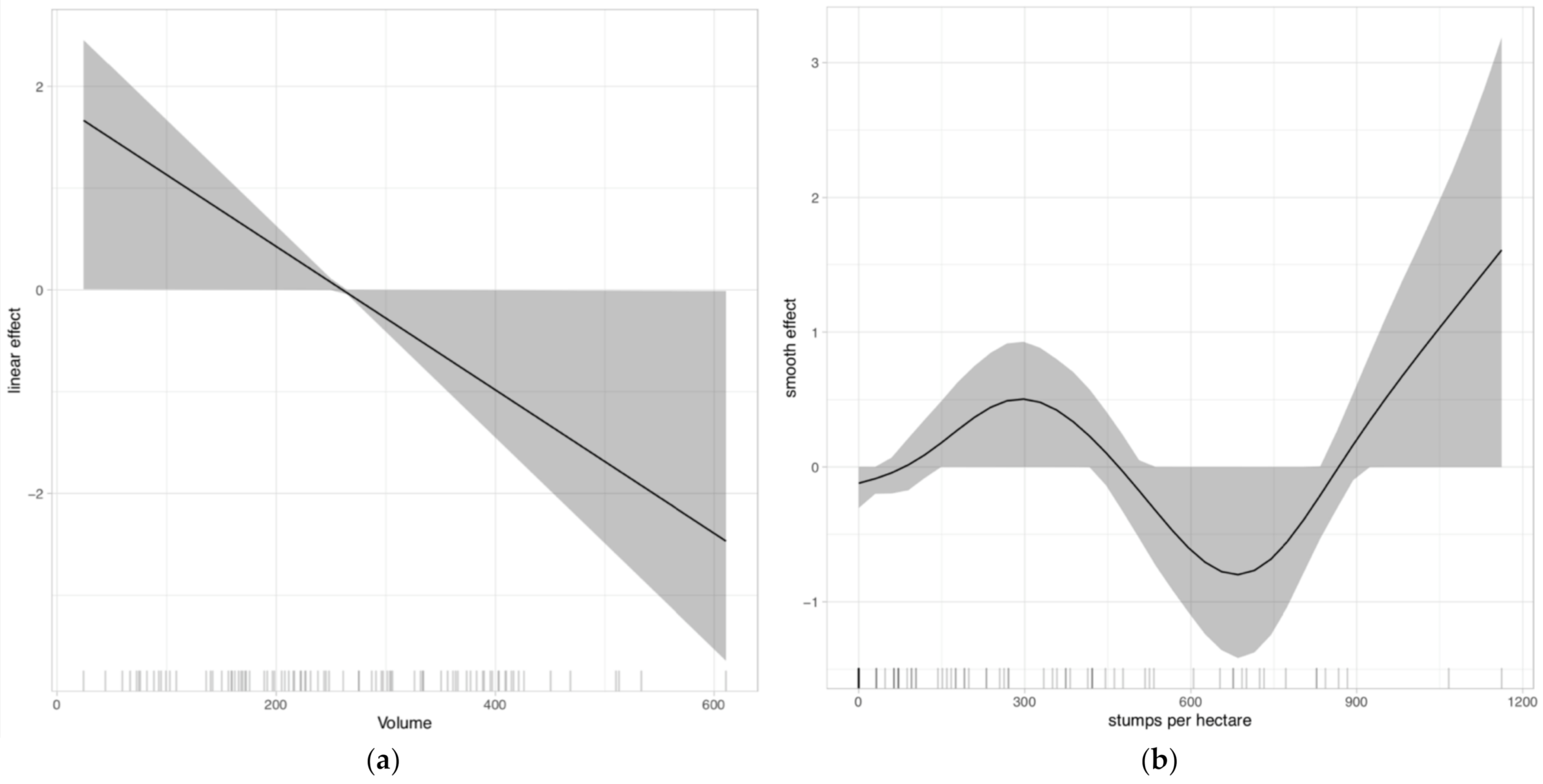
Herbaceous vegetation was positively associated with southern aspects in particular but also northern aspects and gentle slopes, and negatively associated with beech forests and basal area. Occurrence of ants was positively associated with living wood volume (probability of inclusion 0.78) and number of stumps (probability of inclusion 0.74; Figure 3).
We also identified higher decay classes as a key factor directly related to the probability of accumulation of deadwood (Table 5) and, as expected, to ant abundance. For wild ungulates, we failed to find any relationship with forest structural parameters, but occurrence of pellet groups during autumn was the lowest at intermediate elevations (i.e., 900–1600 m a.s.l.) and highest above this limit, and high where karst morphology and limestone substrates predominated.
4. Discussion
This study was the first to attempt an assessment of the functional relationship between characteristics of Apennine forests and the productivity of key foods for Apennine bears. Since beech and oak forests are predominant in our study area, it is not surprising that forest typology exerted the most relevant effect on hard-mast availability. We found negative relationships between basal area of hard-mast-producing species (our proxy of fruit productivity) and both the number of cut stumps and the deadwood decay stage. This suggests that density may be a detrimental factor for radial growth, development of crown area, and fruit production. Deadwood availability is related to high competition in stands with high tree density [84] and the main force of accumulation was forestry, since in the recent past, wood and logging slash were regularly removed [85]. Considering the number of decay classes as an index of forestry operations (i.e., time since the last intervention), hard-mast availability was lower in stands where deadwood was successfully stored (i.e., greater time elapsed since the last forestry operation). Traditionally, in central Italy, deadwood was removed to avoid the risk of forest fires and to limit the potential spread of pathogens. In addition, rural communities used to collect deadwood to be used as fuel. Now that the forests are no longer managed and the mountains are depopulating, dead wood can accumulate, and its degree of decomposition can therefore be an indication of the time of the last intervention. In the studied latitudes and climatic conditions, the decay time is not so fast, especially since we considered in our analysis the largest fraction of dead wood (snags, logs, and stumps). Our results also showed the negative role of overmature coppice in hard-mast productivity; this is probably due to patterns of spatial aggregation of the stems, which are aggregated in stumps. The high density of stems and the vertical layering of these stands produce a higher level of competition for light, [86] therefore affecting the development of the crown [87] and influencing fruit production [88,89]. This trend seems also to be confirmed by local studies of acorns and beechnuts production that indicated a low hard-mast provision in overmature coppice stands or stands in the early stage of conversion Our results suggest that a lower tree density in overmature coppices and irregular high forests could improve hard-mast availability, as also evidenced in an experimental study of Apennine beech coppices under conversion to high forest [90].
Another critical factor affecting hard-mast availability was the level of interspersion of producing species at a local (i.e., bear’s home range scale) and landscape scale. Reflecting a common pattern across the Apennines, we found that the European beech grows in pure stands with a low occurrence of other hard-mast producers, and that the contact zones with oaks depends mainly on slope and aspect [91]. Mixed stands of oak and beech (or distributed in patches) occur on sites where the competitive capacity of beech is reduced and oak can compete successfully. The presence of beech mixtures can negatively affect the oak increment of a basal area [92] proportionally more in closed-canopy forests, where a lower light transmittance creates an unfavorable habitat for heliophilic oaks. We determined that hard-mast-producing species also occurred sporadically in old hornbeam coppices: beech and Turkey oak at the higher altitudes and the downy oak at the lower altitudes. The secondary succession of these stands is only theoretical [93] as there are no studies or data about their evolution. However, [94] showed a decline in light-demanding oaks and an increase in nutrient-demanding shady species after the abandonment of coppicing.
A good interspersion of hard-mast producers is an important indicator of bear habitat quality, as the spatial distribution of food resources strongly affects the size, configuration, and location of bear home ranges at the landscape scale [95,96,97]. Moreover, hard-mast production exhibits large temporal and spatial variation, as this is a pulsed resource that is subject to marked annual fluctuations and occasional mast failures [98,99]. Silvicultural practices can enhance the functional diversity of hard-mast species for bears [100] at a landscape scale, and also ensure supplies of alternate foods in years when the major food source is scarce. To promote oak diffusion, or alternatively to complement beech, hornbeam and mixed old coppice stands (Turkey oak dominated) could be managed by thinning to reduce the tree density removing hornbeam shoots and some old oaks standards around the best oak shoots and secondary species. The removal of some senescent plants, even though this would cause an initial decrease in the production of acorns, could be necessary to initiate new oak stands, contributing to hard-mast production and mitigating future oak losses driven by oak decline and ecological succession [101].
With respect to soft-mast-producing species, we were able to find a significant relationship with slope. Although no studies on soft-mast-producing trees support our result, it is known that slope is negatively related to percent cover of soft-mast shrub and herbaceous species [102], understory plant richness [103], and basal area of trees in plantation sites [104]. Terrain morphology (slope, altitude, and aspect) influences many ecological aspects of forests [105], but we believe that slope in our models captured the effects of more than just a topographic factor. All the soft-mast-producing species that we considered in our study are heliophilous, even though some species (e.g., service trees) are shade-tolerant [106] and able to remain under a dense canopy layer [107,108]. Besides ecological traits, the distribution of soft-mast tree species was likely shaped by past forestry practices designed to eliminate discarded species and enhance production of commercially valued species [109,110]. The joint effect of ecological requirements and the legacy of past management has resulted in a scattered distribution of these species, rarely as an old standard in coppice stands and most frequently in the subcanopies of oak and beech forests. The presence of these sporadic species therefore could be related to past forestry practices such as coppicing and to more open forest structures with greater light availability [111]. It is also negatively related to forests along steep slopes, which are traditionally managed through high tree density and a low rate of silvicultural disturbance, essentially to increase stability and to reduce soil erosion [112]. In such stands, unfavorable conditions exist for soft-mast-producing species, due to the fact that canopy closure reduces light infiltration and increases competitive effects [113,114,115]. As a result, in our study, we observed a very low frequency and often a lack of soft-mast-producing species (Table 6). Being light-demanding and poorly competitive species, their promotion runs through silvicultural practices aimed at reducing competition and enabling an adequate crown development. For example, group selection [116] and tree-oriented silviculture [117] can be enforced even in trees that have long been suppressed [118].
Regarding herbaceous vegetation, ants, and wild ungulates, the results of our models provided only preliminary clues, since the abundance and occurrence of these food items is predictably largely affected by phenology. Nonetheless, we believe that our findings will be useful to inform further investigations and more adequate seasonal sampling. Aspect and slope strongly affected the distribution of herbaceous vegetation. In particular, south-facing aspects were the richest and north-facing ones showed comparable trends, possibly because environmental heterogeneity creates a mosaic of microenvironments shaping different plant communities. Shifts in microclimate across north- and south-facing plant communities are a well-established pattern [119,120,121]. South-facing slopes tend to receive greater insolation, resulting in drier conditions that support thermophile species (e.g., graminoids). North-facing slopes receive less sunlight, creating cool and moist conditions favorable for moisture-loving hygrophile plants. Our findings also suggest that greater slope steepness can negatively influence herb cover, in agreement with similar studies [103,122,123,124]. Slope is an environmental factor known to influence soil moisture (the most important driver for herb cover in forests: [125,126,127,128], air humidity, and soil chemistry [125]). Moreover, we showed that increasing basal area negatively affects herb cover regulating light transmittance through the canopy [129,130,131]. The negative association we revealed with understory cover indicates that light availability on the ground limits the forest herbaceous layer, similarly to other studies [103,120,132,133,134]. We caution that the relationships between basal area and herb cover should be interpreted according to plant functional groups—this caveat being relevant for ‘true forest species’ (with habitat requirements strictly tied to closed canopy forests) for which increased light availability corresponds to a decrease of their incidence [135,136]. For this reason, and by virtue of the complex response of the herbaceous vegetation to thinning [136], it would be necessary to work at the landscape scale and to provide different forest structures with different levels of light requirements.
Concerning the occurrence of animal foods for Apennine bears, we revealed that enhanced occurrence of ants is to be expected in forest stands characterized by low volumes and high tree density, similarly to other Mediterranean mountain environments [137], which are characteristics of young forests and aged coppice. Ants are thermophilic species and their presence in forests is linked to low forest canopy and warmer microclimates [138]. Some species of ants fed upon by bears [26,139] are indeed associated with deadwood [74,76,137,140], which ants use as a substrate or to build nests [141]. In dense forests, high competition levels produce high quantities of deadwood, but in the Apennines, the main driver of deadwood availability is past forest management regimes. As expected, the best predictor of deadwood was the number of decay classes, which is an index of the management forest history of the stand [67,68].
With regard to wild ungulates, we failed to find a robust relationship with forest structure. Although our findings indicated an effect of altitude and soil type on wild ungulate occurrence, the sample size was too low to draw any meaningful conclusion.
In conclusion, the availability of natural food resources is essential to guaranteeing the long-term conservation of the Apennine brown bear, and our study highlights that key bear foods are indeed affected by forest structural and topographical characteristics. The productivity of hard mast was positively associated with both forest typology and high forest system and negatively related to both the time from the last forest utilization and the amount of deadwood. Past forest management was also related to availability of soft-mast-producing species, since forests on steep slopes have been historically managed with high tree densities and low silvicultural disturbance. Our findings also indicate that herb cover was negatively affected by terrain steepness and basal area, while herb productivity was positively affected by northern and southern exposure. Finally, we revealed that forests characterized by low volume and high density corresponded to a higher richness of forest ants. Evidence concerning the effect of forest structure in the occurrence of wild ungulates was less conclusive, but may provide useful hints for further studies.
Our study has some relevant caveats. First, due to logistical constraints, we could collect data only in a single bear dietary season and with no annual replicates. Although we chose the most energetically critical season for bears (i.e., hyperphagia), this was hazardous for assessing the productivity of both hard and soft mast and of herbaceous vegetation, because seed production is characterized by annual variability and occurrence of masting. To overcome this problem, we used basal area, since it has less annual and interannual variability. Second, as we used proxies of key food productivity, our findings are not based on direct measurements of the variables of interest. In order to obtain greater robustness, we encourage future studies to obtain direct measures of productivity and to link resource availability with bear vital rates and population growth [34]. Nevertheless, our study provides general indications on how management of forest structure could enhance productivity of key bear foods. As such, it represents an important first step towards filling the knowledge gap concerning the functional relationship between forest structure and habitat productivity for Apennine bears, and possibly other forest-dwelling species.
Author Contributions
Conceptualization, A.A.R. and P.C.; methodology, A.A.R. and G.J.L.; software, G.J.L.; validation, G.J.L.; formal analysis, A.A.R. and G.J.L.; investigation, A.A.R.; writing—original draft preparation, A.A.R.; writing—review and editing, A.A.R., P.C. and G.J.L.; supervision, P.C.; project administration, A.A.R. and P.C.; funding acquisition, P.C. All authors have read and agreed to the published version of the manuscript.
Funding
This research was part of project “Forest management for the conservation of biodiversity. Examples of actions and guidelines for threatened species” and was funded by “PSL GAL Gran Sasso Velino; Misura 4.1.2—Azione 3C1”.
Institutional Review Board Statement
Not applicable.
Informed Consent Statement
Not applicable.
Data Availability Statement
The data presented in this study are available on request from the corresponding author.
Conflicts of Interest
The authors declare no conflict of interest.
References
- Cardinale, B.J.; Duffy, J.E.; Gonzalez, A.; Hooper, D.U.; Perrings, C.; Venail, P.; Narwani, A.; MacE, G.M.; Tilman, D.; Wardle, D.A.; et al. Biodiversity loss and its impact on humanity. Nature 2012, 486, 59–67. [Google Scholar] [CrossRef] [PubMed]
- Hall, L.S.; Krausman, P.R.; Morrison, M.L. The habitat concept and a plea for standard terminology. Wildl. Soc. Bull. 1997, 25, 173–182. [Google Scholar]
- Grodsky, S.; Moorman, C.; Russell, K. Forest Wildlife Management. In Ecological Forest Management Handbook; Larocque, G.R., Ed.; CRC Press Taylor & Francis Group: New York, NY, USA, 2015; pp. 47–85. [Google Scholar]
- Chaudhary, A.; Burivalova, Z.; Koh, L.P.; Hellweg, S. Impact of Forest Management on Species Richness: Global Meta-Analysis and Economic Trade-Offs. Sci. Rep. 2016, 6, 23954. [Google Scholar] [CrossRef] [PubMed] [Green Version]
- Holbrook, J.D.; Squires, J.R.; Bollenbacher, B.; Graham, R.; Olson, L.E.; Hanvey, G.; Jackson, S.; Lawrence, R.L. Spatio-temporal responses of Canada lynx (Lynx canadensis) to silvicultural treatments in the Northern Rockies, US. For. Ecol. Manag. 2018, 422, 114–124. [Google Scholar] [CrossRef] [Green Version]
- Askins, R.A. Sustaining biological diversity in early successional communities: The challenge of managing unpopular habitats. Wildl. Soc. Bull. 2001, 29, 407–412. [Google Scholar]
- Paillet, Y.; Bergès, L.; Hjältén, J.; Odor, P.; Avon, C.; Bernhardt-Römermann, M.; Bijlsma, R.-J.; De Bruyn, L.; Fuhr, M.; Grandin, U.; et al. Biodiversity differences between managed and unmanaged forests: Meta-analysis of species richness in Europe. Conserv. Biol. 2010, 24, 101–112. [Google Scholar] [CrossRef]
- Riffell, S.; Verschuyl, J.; Miller, D.; Wigley, T.B. Biofuel harvests, coarse woody debris, and biodiversity—A meta-analysis. For. Ecol. Manag. 2011, 261, 878–887. [Google Scholar] [CrossRef]
- Fedrowitz, K.; Koricheva, J.; Baker, S.C.; Lindenmayer, D.B.; Palik, B.; Rosenvald, R.; Beese, W.; Franklin, J.F.; Kouki, J.; Macdonald, E.; et al. Can retention forestry help conserve biodiversity? A meta-analysis. J. Appl. Ecol. 2014, 51, 1669–1679. [Google Scholar] [CrossRef] [Green Version]
- Verschuyl, J.; Riffell, S.; Miller, D.; Wigley, T.B. Biodiversity response to intensive biomass production from forest thinning in North American forests—A meta-analysis. For. Ecol. Manag. 2011, 261, 221–232. [Google Scholar] [CrossRef]
- Franklin, C.M.A.; Macdonald, S.E.; Nielsen, S.E. Can retention harvests help conserve wildlife? Evidence for vertebrates in the boreal forest. Ecosphere 2019, 10, e02632. [Google Scholar] [CrossRef]
- Fisher, J.; Wilkinson, L. The response of mammals to forest fire and timber harvest in the North American boreal forest. Mamm. Rev. 2005, 35, 51–81. [Google Scholar] [CrossRef]
- Kearney, S.P.; Coops, N.C.; Stenhouse, G.B.; Nielsen, S.E.; Hermosilla, T.; White, J.C.; Wulder, M.A. Grizzly bear selection of recently harvested forests is dependent on forest recovery rate and landscape composition. For. Ecol. Manag. 2019, 449, 117459. [Google Scholar] [CrossRef]
- Schwenk, W.S.; Donovan, T.; Keeton, W.S.; Nunery, J.S. Carbon storage, timber production, and biodiversity: Comparing ecosystem services with multi-criteria decision analysis. Ecol. Appl. 2012, 22, 1612–1627. [Google Scholar] [CrossRef]
- Holbrook, J.D.; Squires, J.R.; Bollenbacher, B.; Graham, R.; Olson, L.E.; Hanvey, G.; Jackson, S.; Lawrence, R.L.; Savage, S.L. Management of forests and forest carnivores: Relating landscape mosaics to habitat quality of Canada lynx at their range periphery. For. Ecol. Manag. 2019, 437, 411–425. [Google Scholar] [CrossRef]
- Ciucci, P.; Gervasi, V.; Boitani, L.; Boulanger, J.; Paetkau, D.; Prive, R.; Tosoni, E. Estimating abundance of the remnant Apennine brown bear population using multiple noninvasive genetic data sources. J. Mammal. 2015, 96, 206–220. [Google Scholar] [CrossRef] [Green Version]
- Benazzo, A.; Trucchi, E.; Cahill, J.A.; Delser, P.M.; Mona, S.; Fumagalli, M.; Bunnefeld, L.; Cornetti, L.; Ghirotto, S.; Girardi, M.; et al. Survival and divergence in a small group: The extraordinary genomic history of the endangered Apennine brown bear stragglers. Proc. Natl. Acad. Sci. USA 2017, 114, E9589–E9597. [Google Scholar] [CrossRef] [Green Version]
- Gervasi, V.; Ciucci, P. Demographic projections of the Apennine brown bear population Ursus arctos marsicanus (Mammalia: Ursidae) under alternative management scenarios. Eur. Zool. J. 2018, 85, 242–252. [Google Scholar] [CrossRef] [Green Version]
- Ciucci, P.; Altea, T.; Antonucci, A.; Chiaverini, L.; Di Croce, A.; Fabrizio, M.; Forconi, P.; Latini, R.; Maiorano, L.; Monaco, A.; et al. Distribution of the brown bear (Ursus arctos marsicanus) in the central apennines, Italy, 2005–2014. Hystrix 2017, 28. [Google Scholar] [CrossRef]
- Maiorano, L.; Chiaverini, L.; Falco, M.; Ciucci, P. Combining multi-state species distribution models, mortality estimates, and landscape connectivity to model potential species distribution for endangered species in human dominated landscapes. Biol. Conserv. 2019, 237, 19–27. [Google Scholar] [CrossRef]
- Anonymous. Piano d ’Azione Nazionale per la Tutela Dell’orso Bruno Marsicano-PATOM; Ministero dell’ Ambiente-ISPRA: Roma, Italy, 2011; Volume 37. [Google Scholar]
- Falcucci, A.; Ciucci, P.; Maiorano, L.; Gentile, L.; Boitani, L. Assessing habitat quality for conservation using an integrated occurrence-mortality model. J. Appl. Ecol. 2009, 46, 600–609. [Google Scholar] [CrossRef]
- Posillico, M.; Meriggi, A.; Pagnin, E.; Lovari, S.; Russo, L. A habitat model for brown bear conservation and land use planning in the central Apennines. Biol. Conserv. 2004, 118, 141–150. [Google Scholar] [CrossRef]
- Tosoni, E.; Boitani, L.; Gentile, L.; Gervasi, V.; Latini, R.; Ciucci, P. Assessment of key reproductive traits in the Apennine brown bear population. Ursus 2017, 28, 105. [Google Scholar] [CrossRef]
- Gervasi, V.; Boitani, L.; Paetkau, D.; Posillico, M.; Randi, E.; Ciucci, P. Estimating survival in the Apennine brown bear accounting for uncertainty in age classification. Popul. Ecol. 2017, 59, 119–130. [Google Scholar] [CrossRef]
- Ciucci, P.; Tosoni, E.; Di Domenico, G.; Quattrociocchi, F.; Boitani, L. Seasonal and annual variation in the food habits of Apennine brown bears, central Italy. J. Mammal. 2014, 95, 572–586. [Google Scholar] [CrossRef] [Green Version]
- Larsen, T.A.; Nielsen, S.E.; Cranston, J.; Stenhouse, G.B. Do remnant retention patches and forest edges increase grizzly bear food supply? For. Ecol. Manag. 2019, 433, 741–761. [Google Scholar] [CrossRef]
- Nielsen, S.E.; McDermid, G.; Stenhouse, G.B.; Boyce, M.S. Dynamic wildlife habitat models: Seasonal foods and mortality risk predict occupancy-abundance and habitat selection in grizzly bears. Biol. Conserv. 2010, 143, 1623–1634. [Google Scholar] [CrossRef]
- McLellan, B.N. Some mechanisms underlying variation in vital rates of grizzly bears on a multiple use landscape. J. Wildl. Manag. 2015, 79, 749–765. [Google Scholar] [CrossRef]
- Bojarska, K.; Selva, N. Spatial patterns in brown bear Ursus arctos diet: The role of geographical and environmental factors. Mamm. Rev. 2012, 42, 120–143. [Google Scholar] [CrossRef]
- Nielsen, S.E.; Boyce, M.S.; Stenhouse, G.B. Grizzly bears and forestry I. Selection of clearcuts by grizzly bears in west-central Alberta, Canada Scott. For. Ecol. Manag. 2004, 199, 51–65. [Google Scholar] [CrossRef]
- Clevenger, A.P.; Purroy, F.J.; Pelton, M.R. Food Habits of Brown Bears (Ursus arctos) in the Cantabrian Mountains, Spain. J. Mammal. 1992, 73, 415–421. [Google Scholar] [CrossRef]
- Costello, C.M.C.; Jones, D.E.; Inman, R.R.M.; Inman, K.H.; Bruce, C.; Quigley, H.B. Relationship of variable mast production to American black bear reproductive parameters in New Mexico. Ursus 2003, 14, 1–16. [Google Scholar]
- Reynolds-Hogland, M.J.; Pacifici, L.B.; Mitchell, M.S. Linking resources with demography to understand resource limitation for bears. J. Appl. Ecol. 2007, 44, 1166–1175. [Google Scholar] [CrossRef]
- Hashimoto, Y.; Kaji, M.; Sawada, H.; Takatsuki, S. Five-year study on the autumn food habits of the Asiatic black bear in relation to nut production. Ecol. Res. 2003, 18, 485–492. [Google Scholar] [CrossRef]
- Atkinson, S.N.; Ramsay, M.A. The Effects of Prolonged Fasting of the Body Composition and Reproductive Success of Female Polar Bears (Ursus maritimus). Funct. Ecol. 1995, 9, 559. [Google Scholar] [CrossRef]
- Tosoni, E.; Boitani, L.; Mastrantonio, G.; Latini, R.; Ciucci, P. Counts of unique females with cubs in the Apennine brown bear population, 2006–2014. Ursus 2017, 28, 1–14. [Google Scholar] [CrossRef]
- Mitchell, M.S.; Powell, R.A. Response of Black Bears to Forest Management in the Southern Appalachian Mountains. J. Wildl. Manag. 2003, 67, 692. [Google Scholar] [CrossRef]
- Brodeur, V.; Ouellet, J.-P.; Courtois, R.; Fortin, D. Habitat selection by black bears in an intensively logged boreal forest. Can. J. Zool. 2008, 86, 1307–1316. [Google Scholar] [CrossRef]
- Davis, H.; Hamilton, A.N.; Harestad, A.S.; Weir, R.D. Longevity and reuse of black bear dens in managed forests of coastal British Columbia. J. Wildl. Manag. 2012, 76, 523–527. [Google Scholar] [CrossRef]
- Zager, P.; Jonkel, C.; Habeck, J. Logging and Wildfire Influence on Grizzly Bear Habitat in Northwestern Montana. Int. Conf. Bear Res. Manag. 1980, 5, 124–132. [Google Scholar] [CrossRef]
- Wielgus, R.B.; Vernier, P.R. Grizzly bear selection of managed and unmanaged forests in the Selkirk Mountains. Can. J. For. Res 2003, 33, 822–829. [Google Scholar] [CrossRef]
- Nielsen, S.E.; Munro, R.H.M.; Bainbridge, E.L.; Stenhouse, G.B.; Boyce, M.S. Grizzly bears and forestry II. Distribution of grizzly bear foods in clearcuts of west-central Alberta, Canada. For. Ecol. Manag. 2004, 199, 67–82. [Google Scholar] [CrossRef]
- Braid, A.C.R.; Manzer, D.; Nielsen, S.E. Wildlife habitat enhancements for grizzly bears: Survival rates of planted fruiting shrubs in forest harvests. For. Ecol. Manag. 2016, 369, 144–154. [Google Scholar] [CrossRef]
- Souliere, C.M.; Coogan, S.C.P.; Stenhouse, G.B.; Nielsen, S.E. Harvested forests as a surrogate to wildfires in relation to grizzly bear food- supply in west-central Alberta. For. Ecol. Manag. 2020, 456, 117685. [Google Scholar] [CrossRef]
- Ciucci, P.; Boitani, L. The Apennine brown bear: A critical review of its status and conservation problems. Ursus 2008, 19, 130–145. [Google Scholar] [CrossRef]
- Kane, V.R.; Lutz, J.A.; Alina Cansler, C.; Povak, N.A.; Churchill, D.J.; Smith, D.F.; Kane, J.T.; North, M.P. Water balance and topography predict fire and forest structure patterns. For. Ecol. Manag. 2015, 338, 1–13. [Google Scholar] [CrossRef]
- Tateno, R.; Takeda, H. Forest structure and tree species distribution in relation to topography-mediated heterogeneity of soil nitrogen and light at the forest floor. Ecol. Res. 2003, 18, 559–571. [Google Scholar] [CrossRef]
- Underwood, E.C.; Viers, J.H.; Quinn, J.F.; North, M. Using topography to meet wildlife and fuels treatment objectives in fire-suppressed landscapes. Environ. Manag. 2010, 46, 809–819. [Google Scholar] [CrossRef] [Green Version]
- Morini, P.; Pinchera, F.P.; Nucci, L.M.; Ferlini, F.; Cecala, S.; Di Nino, O.; Penteriani, V. Brown bears in Central Italy: A 15-year study on bear occurrence. Eur. Zool. J. 2017, 84, 26–33. [Google Scholar] [CrossRef]
- Ministero dell’Ambiente e della Tutela del Territorio e del Mare Carta Fitoclimatica d’Italia. Available online: http://www.pcn.minambiente.it/viewer/index.php?services=Fitoclima (accessed on 7 April 2020).
- Collalti, D.; D’Alessandro, L.; Marchetti, M.; Sebastiani, A. La Carta Tipologico-Forestale Della Regione Abruzzo. Volume Generale; Regione Abruzzo: L’Aquila, Italy, 2009; p. 340. [Google Scholar]
- Vacchiano, G.; Garbarino, M.; Lingua, E.; Motta, R. Forest dynamics and disturbance regimes in the Italian Apennines. For. Ecol. Manag. 2017, 388, 57–66. [Google Scholar] [CrossRef] [Green Version]
- Nocentini, S. Structure and management of beech (Fagus sylvatica L.) forests in Italy. iForest-Biogeosci. For. 2009, 2, 105–113. [Google Scholar] [CrossRef] [Green Version]
- Costantini, E.A.C.; Dazzi, C. The Soils of Italy; Springer: Dordrecht, The Netherlands, 2013; ISBN 9400756429. [Google Scholar]
- McElhinny, C.; Gibbons, P.; Brack, C.; Bauhus, J. Forest and woodland stand structural complexity: Its definition and measurement. For. Ecol. Manag. 2005, 218, 1–24. [Google Scholar] [CrossRef]
- Pretzsch, H. Structural Diversity As a Result of silviculural operations. Lesnictvi-Forestry 1998, 44, 429–439. [Google Scholar]
- Latham, P.A.; Zuuring, H.R.; Coble, D.W. A method for quantifying vertical forest structure. For. Ecol. Manag. 1998, 104, 157–170. [Google Scholar] [CrossRef]
- Kutsch, W.L.; Wirth, C.; Kattge, J.; Nöllert, S.; Herbst, M.; Kappen, L. Old-Growth Forests: Function, Fate and Value; Wirth, C., Gleixner, G., Heimann, M., Eds.; Springer: Berlin/Heidelberg, Germany, 2009; pp. 57–79. ISBN 978-3-540-92706-8. [Google Scholar]
- Shannon, C. A mathematical theory of communication. Bell Syst. Technol. J. 1948, 27, 379–423. [Google Scholar] [CrossRef] [Green Version]
- Simpson, E.H. Measurement of diversity. Nature 1949, 163, 688. [Google Scholar] [CrossRef]
- Pielou, E.C. The measurement of diversity in different types of biolagical collections. J. Theor. Biol. 1966, 13, 131–144. [Google Scholar] [CrossRef]
- Tabacchi, G.; Di Cosmo, L.; Gasparini, P.; Morelli, S. Stima del Volume e Della Fitomassa Delle Principali Specie Forestali Italiane, Equazioni di Previsione, Tavole del Volume e Tavole Della Fitomassa Arborea Epigea; Consiglio per la Ricerca e la Sperimentazione in Agricoltura Unità di Ricerca per il Monitoraggio e la Pianificazione Forestale: Trento, Italy, 2011; ISBN 9788897081111.
- West, P.W. Stem Volume. In Tree and Forest Measurement; Springer: Berlin/Heidelberg, Germany, 2009; pp. 23–32. ISBN 978-3-540-95966-3. [Google Scholar]
- Hunter, M.L.J. Wildlife, Forests, and Forestry: Principles of Managing Forests for Biological Diversity; Prentice-Hall: Hoboken, NJ, USA, 1990. [Google Scholar]
- Cindolo, C.; Petriccione, B. Progetto Biosoil—Biodiversity. Valutazione Della Biodiversità Forestale Sulla Rete Sistematica di Livello I. Manuale Nazionale, Italia; Corpo Forestale dello Stato: Roma, Italy, 2006. [Google Scholar]
- Stokland, J.N. The coarse woody debris profile: An archive of recent history and an important biodiversity. Ecol. Bull. 2001, 49, 71–83. [Google Scholar] [CrossRef]
- Rouvinen, S.; Rautiainen, A.; Kouki, J. A relation between historical forest use and current dead woody material in a boreal protected old-growth forest in Finland. Silva Fenn. 2005, 39, 21–36. [Google Scholar] [CrossRef] [Green Version]
- Greenberg, C.H. Individual variation in acorn production by five species of southern Appalachian oaks. For. Ecol. Manag. 2000, 132, 199–210. [Google Scholar] [CrossRef]
- Molina, M.; Pardo-de-santayana, M.; Aceituno, L.; Morales, R.; Tardío, J. Fruit production of strawberry tree (Arbutus unedo L.) in two Spanish forests. Forestry 2011, 84, 419–429. [Google Scholar] [CrossRef]
- Potena, G.; Sammarone, L.; Posillico, M.; Romano, M.; Consalvo, M. Fruttificazione del Faggio (Fagus sylvatica) e delle Querce (Quercus cerris, Q. pubescens) nel Parco Nazionale d’Abruzzo, Lazio e Molise e Zona di Protezione Esterna Nel 2007; Ufficio Foreste Demaniali di Castel di Sangro: L’Aquila, Italy, 2008. [Google Scholar]
- Canfield, R.H. Application of the line interception method in sampling range vegetation. J. For. 1941, 39, 34–40. [Google Scholar]
- Bonham, C.D. Measurements for Terrestrial Vegetation, 2nd ed.; John Wiley and Sons: New York, NY, USA, 2013; ISBN 9780470972588. [Google Scholar]
- Alvarado, M. Habitat correlates of ant assemblages in different forests of the South Pannonian Plain. Tiscia 2000, 32, 35–42. [Google Scholar]
- Frank, S.C.; Steyaert, S.M.J.G.; Swenson, J.E.; Storch, I.; Kindberg, J.; Barck, H.; Zedrosser, A. A “clearcut” case? Brown bear selection of coarse woody debris and carpenter ants on clearcuts. For. Ecol. Manag. 2015, 348, 164–173. [Google Scholar] [CrossRef] [PubMed] [Green Version]
- Higgins, R.J.; Lindgren, B.S. The Fine Scale Physical Attributes of Coarse Woody Debris and Effects of Surrounding Stand Structure on Its Utilization by Ants (Hymenoptera: Formicidae) in British Columbia, Canada; General Technical Report SRS-93; Department of Agriculture, Forest Service, Southern Research Station: Asheville, NC, USA, 2006; pp. 67–74.
- Zhao, Y.; Staudenmayer, J.; Coull, B.A.; Wand, M.P. General Design Bayesian Generalized Linear Mixed Models. Stat. Sci. 2006, 21, 35–51. [Google Scholar] [CrossRef] [Green Version]
- Spiegelhalter, D.J.; Best, N.G.; Carlin, B.P.; van der Linde, A. Bayesian Measures of Model Complexity and fit. J. R. Stat. Soc. Ser. B Stat. Methodol. 2002, 64, 583–639. [Google Scholar] [CrossRef] [Green Version]
- Wakefield, J. Bayesian and Frequentist Regression Methods; Springer: New York, NY, USA, 2013; ISBN 1441909257. [Google Scholar]
- Wood, S.N. Generalized additive models: An introduction with R. Chapman and Hall/CRC. Texts Stat. Sci. 2006, 67, 391. [Google Scholar]
- Scheipl, F. spikeSlabGAM: Bayesian Variable Selection, Model Choice and Regularization for Generalized Additive Mixed Models in R. J. Stat. Softw. 2011, 43, 1–24. [Google Scholar] [CrossRef] [Green Version]
- Ishwaran, H.; Rao, J.S. Spike and Slab Variable Selection: Frequentist and Bayesian Strategies. Ann. Stat. 2005, 33, 730–773. [Google Scholar] [CrossRef] [Green Version]
- Plummer, M. JAGS: A Program for Analysis of Bayesian Graphical Models Using Gibbs Sampling. In Proceedings of the 3rd International Workshop on Distributed Statistical Computing, Vienna, Austria, 20–22 March 2003. [Google Scholar]
- Meyer, P.; Schmidt, M. Accumulation of dead wood in abandoned beech (Fagus sylvatica L.) forests in northwestern Germany. For. Ecol. Manag. 2011, 261, 342–352. [Google Scholar] [CrossRef]
- Castagneri, D.; Garbarino, M.; Berretti, R.; Motta, R. Site and stand effects on coarse woody debris in montane mixed forests of Eastern Italian Alps. For. Ecol. Manag. 2010, 260, 1592–1598. [Google Scholar] [CrossRef] [Green Version]
- Scolastri, A.; Cancellieri, L.; Iocchi, M.; Cutini, M. Old coppice versus high forest: The impact of beech forest management on plant species diversity in central Apennines (Italy). J. Plant Ecol. 2017, 10, 271–280. [Google Scholar] [CrossRef] [Green Version]
- Juchheim, J.; Annighöfer, P.; Ammer, C.; Calders, K.; Raumonen, P.; Seidel, D. How management intensity and neighborhood composition affect the structure of beech (Fagus sylvatica L.) trees. Trees Struct. Funct. 2017, 31, 1723–1735. [Google Scholar] [CrossRef]
- Abrahamson, W.G.; Layne, J.N. Long-term patterns of acorn production for five oak species in xeric Florida uplands. Ecology 2003, 84, 2476–2492. [Google Scholar] [CrossRef]
- Kamler, J.; Dobrovolný, L.; Drimaj, J.; Kadavý, J.; Kneifl, M.; Adamec, Z.; Knott, R.; Martiník, A.; Plhal, R.; Zeman, J.; et al. The impact of seed predation and browsing on natural sessile oak regeneration under different light conditions in an over-aged coppice stand. iForest-Biogeosci. For. 2016, 9, 569–576. [Google Scholar] [CrossRef] [Green Version]
- Cutini, A.; Chianucci, F.; Giannini, T. Effetti del trattamento selvicolturale su caratteristiche della copertura, produzione di lettiera e di seme in cedui di faggio in conversione. Ann. CRA 2009, 36, 109–124. [Google Scholar]
- Pignatti, S. La faggeta. In I Boschi d’Italia. Sinecologia e Biodiversità; UTET: Torino, Italy, 1998; p. 673. [Google Scholar]
- Hein, S.; Dhôte, J.-F. Effect of species composition, stand density and site index on the basal area increment of oak trees (Quercus sp.) in mixed stands with beech (Fagus sylvatica L.) in northern France. Ann. For. Sci. 2006, 63, 457–467. [Google Scholar] [CrossRef] [Green Version]
- Pignatti, G.; Terzuolo, P.G.; Varese, P.; Semerari, P.; Lombardi, V. Criteri per la definizione di tipi forestali nei boschi dell’ Appennino meridionale. Forest 2004, 1, 112–127. [Google Scholar] [CrossRef]
- Müllerová, J.; Hédl, R.; Szabó, P. Coppice abandonment and its implications for species diversity in forest vegetation. For. Ecol. Manag. 2015, 343, 88–100. [Google Scholar] [CrossRef] [Green Version]
- Mangipane, L.S.; Belant, J.L.; Hiller, T.L.; Colvin, M.E.; Gustine, D.D.; Mangipane, B.A.; Hilderbrand, G.V. Influences of landscape heterogeneity on home-range sizes of brown bears. Mamm. Biol. 2018, 88, 1–7. [Google Scholar] [CrossRef]
- Mitchell, M.S.; Powell, R.A. Optimal use of resources structures home ranges and spatial distribution of black bears. Anim. Behav. 2007, 74, 219–230. [Google Scholar] [CrossRef]
- Mitchell, M.S.; Powell, R.A. A mechanistic home range model for optimal use of spatially distributed resources. Ecol. Modell. 2004, 177, 209–232. [Google Scholar] [CrossRef]
- Koenig, W.D.; Knops, J.M.H. Patterns of Annual Seed Production by Northern Hemisphere Trees: A Global Perspective. Am. Nat. 2000, 155, 59–69. [Google Scholar] [CrossRef]
- Bogdziewicz, M.; Steele, M.A.; Marino, S.; Crone, E.E. Correlated seed failure as an environmental veto to synchronize reproduction of masting plants. New Phytol. 2018, 219, 98–108. [Google Scholar] [CrossRef] [PubMed] [Green Version]
- Garshelis, D.L.; Noyce, K.V. Seeing the World through the Nose of a Bear—Diversity of Foods Fosters Behavioral and Demographic Stability. In Wildlife Science Linking Ecological Theory and Management Applications; CRC Press Taylor & Francis Group: New York, NY, USA, 2007; pp. 139–164. [Google Scholar] [CrossRef]
- Olson, M.G.; Wolf, A.J.; Jensen, R.G. Influence of Forest Management on Acorn Production in the Southeastern Missouri Ozarks: Early Results of a Long-Term Ecosystem Experiment. Open J. For. 2015, 5, 568–583. [Google Scholar] [CrossRef] [Green Version]
- Reynolds-Hogland, M.J.; Mitchell, M.S.; Powell, R.A. Spatio-temporal availability of soft mast in clearcuts in the Southern Appalachians. For. Ecol. Manag. 2006, 237, 103–114. [Google Scholar] [CrossRef]
- Fredericksen, T.S.; Ross, B.D.; Hoffman, W.; Morrison, M.L.; Beyea, J.; Johnson, B.N.; Lester, M.B.; Ross, E. Short-term understory plant community responses to timber-harvesting intensity on non-industrial private forestlands in Pennsylvania. For. Ecol. Manag. 1999, 116, 129–139. [Google Scholar] [CrossRef]
- Saremi, H.; Kumar, L.; Turner, R.; Stone, C.; Melville, G. Impact of local slope and aspect assessed from LiDAR records on tree diameter in radiata pine (Pinus radiata D. Don) plantations. Ann. For. Sci. 2014, 71, 771–780. [Google Scholar] [CrossRef]
- Melini, D. A spatial model for sporadic tree species distribution in support of tree oriented silviculture. Ann. Silvic. Res. 2013, 37, 64–68. [Google Scholar]
- Raspe, O.; Findlay, C.; Jacquemart, L. Sorbus aucuparia L. J. Ecol. 2000, 910–930. [Google Scholar] [CrossRef]
- Pyttel, P.; Kunz, J.; Bauhus, J. Growth, regeneration and shade tolerance of the Wild Service Tree (Sorbus torminalis (L.) Crantz) in aged oak coppice forests. Trees Struct. Funct. 2013, 27, 1609–1619. [Google Scholar] [CrossRef]
- Paganová, V. Ecological requirements of wild service tree (Sorbus torminalis [L.] CRANTZ.) and service tree (Sorbus domestica L.) in relation with their utilizatiion in forestry and landscape. J. For. Sci. 2008, 54, 216–226. [Google Scholar] [CrossRef] [Green Version]
- Bernetti, G. Note sul trattamento delle fustaie di Faggio. Trattamento delle faggete in Italia: Dal metodo scientifico all’empirismo dei nostri giorni. I Georg. Quad. 2012, 2012-III, 7–11. [Google Scholar]
- Hertel, A.G.; Steyaert, S.M.J.G.; Zedrosser, A.; Mysterud, A.; Lodberg-Holm, H.K.; Gelink, H.W.; Kindberg, J.; Swenson, J.E. Bears and berries: Species-specific selective foraging on a patchily distributed food resource in a human-altered landscape. Behav. Ecol. Sociobiol. 2016, 70, 831–842. [Google Scholar] [CrossRef] [Green Version]
- Rasmussen, K.K.; Kollmann, J. Defining the habitat niche of Sorbus torminalis from phytosociological relevés along a latitudinal gradient. Phytocoenologia 2004, 34, 639–662. [Google Scholar] [CrossRef]
- Piussi, P. Selvicoltura Generale; UTET: Torino, Italy, 1994; ISBN 880204869X.
- Perry, R.W.; Thill, R.E.; Peitz, D.G.; Tappe, P.A. Effect of different silvicultural systems on initial soft mast production. Wildl. Soc. Bull. 1999, 27, 915–923. [Google Scholar]
- Greenberg, C.H.; States, U.; Service, F.; Creek, B.; Forest, E.; Road, B. Fruit Production in Mature and Recently Regenerated Forests of the Appalachians. J. Wildl. Manag. 2007, 71, 321–335. [Google Scholar] [CrossRef]
- Greenberg, C.H.; Levey, D.J.; Kwit, C.; Mccarty, J.P.; Pearson, S.F.; Sargent, S.; Kilgo, J. Long-term patterns of fruit production in five forest types of the south carolina upper coastal plain. J. Wildl. Manag. 2012, 76, 1036–1046. [Google Scholar] [CrossRef]
- Spiecker, H.; Sebastian, H.; Makkonnen-Spiecker, K.; Thies, M. Valuable Broadleaved Forests in Europe; EFI Research Report 22; Brill: Leiden, The Netherlands; Boston, MA, USA; Köln, Germany, 2009; ISBN 978-90-04-16795-7. [Google Scholar]
- Manetti, M.C.; Becagli, C.; Sansone, D.; Pelleri, F. Tree-oriented silviculture: A new approach for coppice stands. iForest-Biogeosci. For. 2016, 9, 791–800. [Google Scholar] [CrossRef] [Green Version]
- Pyttel, P.; Kunz, J.; Großmann, J. Growth of Sorbus torminalis after release from prolonged suppression. Trees Struct. Funct. 2019, 33, 1549–1557. [Google Scholar] [CrossRef]
- Warren, R.J. Mechanisms driving understory evergreen herb distributions across slope aspects: As derived from landscape position. Plant Ecol. 2008, 198, 297–308. [Google Scholar] [CrossRef]
- Gracia, M.; Montané, F.; Piqué, J.; Retana, J. Overstory structure and topographic gradients determining diversity and abundance of understory shrub species in temperate forests in central Pyrenees (NE Spain). For. Ecol. Manag. 2007, 242, 391–397. [Google Scholar] [CrossRef]
- Small, C.J.; McCarthy, B.C. Spatial and temporal variability of herbaceous vegetation in an eastern deciduous forest. Plant Ecol. 2002, 164, 37–48. [Google Scholar] [CrossRef]
- Horvat, V.; Biurrun, I.; García-Mijangos, I. Herb layer in silver fir—Beech forests in the western Pyrenees: Does management affect species diversity? For. Ecol. Manag. 2017, 385, 87–96. [Google Scholar] [CrossRef]
- Pinder, J.E.; Kroh, G.C.; White, J.D.; Basham May, A.M. The relationships between vegetation type and topography in Lassen Volcanic National Park. Plant Ecol. 1997, 131, 17–29. [Google Scholar] [CrossRef]
- Small, C.J.; McCarthy, B.C. Relationship of understory diversity to soil nitrogen, topographic variation, and stand age in an eastern oak forest, USA. For. Ecol. Manag. 2005, 217, 229–243. [Google Scholar] [CrossRef]
- Leuschner, C.; Lendzion, J. Air humidity, soil moisture and soil chemistry as determinants of the herb layer composition in European beech forests. J. Veg. Sci. 2009, 20, 288–298. [Google Scholar] [CrossRef]
- Hokkanen, P.J. Environmental patterns and gradients in the vascular plants and bryophytes of eastern Fennoscandian herb-rich forests. For. Ecol. Manag. 2006, 229, 73–87. [Google Scholar] [CrossRef]
- North, M.; Oakley, B.; Fiegener, R.; Gray, A.; Barbour, M. Influence of light and soil moisture on Sierran mixed-conifer understory communities. Plant Ecol. 2005, 177, 13–24. [Google Scholar] [CrossRef]
- Gálhidy, L.; Mihók, B.; Hagyó, A.; Rajkai, K.; Standovár, T. Effects of gap size and associated changes in light and soil moisture on the understorey vegetation of a Hungarian beech forest. Plant Ecol. 2006, 183, 133–145. [Google Scholar] [CrossRef]
- Gabriela Sonohat; Philippe Balandier; Felix Ruchaud Predicting solar radiation transmittance in the understory of even-aged coniferous stands in temperate forests. Ann. For. Sci. 2004, 61, 629–641. [CrossRef] [Green Version]
- Hale, S.E. The effect of thinning intensity on the below-canopy light environment in a Sitka spruce plantation. For. Ecol. Manag. 2003, 179, 341–349. [Google Scholar] [CrossRef]
- Page, L.M.; Cameron, A.D.; Clarke, G.C. Influence of overstorey basal area on density and growth of advance regeneration of Sitka spruce in variably thinned stands. For. Ecol. Manag. 2001, 151, 25–35. [Google Scholar] [CrossRef]
- Campione, M.A.; Nagel, L.M.; Webster, C.R. Herbaceous-Layer Community Dynamics along a Harvest-Intensity Gradient after 50 Years of Consistent Management. Open J. For. 2012, 02, 97–106. [Google Scholar] [CrossRef]
- Hofmeister, J.; Hosek, J.; Brabec, M.; Hedl, R.; Modry, M. Strong influence of long-distance edge effect on herb-layer vegetation in forest fragments in an agricultural landscape. Perspect. Plant Ecol. Evol. Syst. 2013, 15, 293–303. [Google Scholar] [CrossRef]
- Coll, L.; González-Olabarria, J.R.; Mola-Yudego, B.; Pukkala, T.; Messier, C. Predicting understory maximum shrubs cover using altitude and overstory basal area in different Mediterranean forests. Eur. J. For. Res. 2011, 130, 55–65. [Google Scholar] [CrossRef] [Green Version]
- Vockenhuber, E.A.; Scherber, C.; Langenbruch, C.; Meiner, M.; Seidel, D.; Tscharntke, T. Tree diversity and environmental context predict herb species richness and cover in Germany’s largest connected deciduous forest. Perspect. Plant Ecol. Evol. Syst. 2011, 13, 111–119. [Google Scholar] [CrossRef]
- Decocq, G.; Aubert, M.; Dupont, F.; Alard, D.; Saguez, R.; Wattez-franger, A.; Foucault, B.D.E.; Delelis-dusollier, A. Plant diversity in a managed temperate deciduous forest: Understorey response to two silvicultural systems. J. Appl. Ecol. 2004, 41, 1065–1079. [Google Scholar] [CrossRef]
- Arnan, X.; Gracia, M.; Lluis, C.; Retana, J. Forest management conditioning ground ant community structure and composition in temperate conifer forests in the Pyrenees Mountains. For. Ecol. Manag. 2009, 258, 51–59. [Google Scholar] [CrossRef]
- Grevé, M.E.; Hager, J.; Weisser, W.W.; Schall, P.; Gossner, M.M.; Feldhaar, H. Effect of forest management on temperate ant communities. Ecosphere 2018, 9, e02303. [Google Scholar] [CrossRef]
- Noyce, K.V.; Kannowski, P.B.; Riggs, M.R. Black bears as ant-eaters: Seasonal associations between bear myrmecophagy and ant ecology in north-central Minnesota. Can. J. Zool. 1997, 75, 1671–1686. [Google Scholar] [CrossRef]
- Warren, R.J.; Bradford, M.A. Ant colonization and coarse woody debris decomposition in temperate forests. Insectes Soc. 2011, 59, 215–221. [Google Scholar] [CrossRef]
- King, J.R.; Warren, R.J.; Maynard, D.S.; Bradford, M.A. Ants: Ecology and Impacts in Dead Wood. In Saproxylic Insects: Diversity, Ecology and Conservation; Ulyshen, M.D., Ed.; Springer: Cham, Switzerland, 2018; pp. 237–262. ISBN 978-3-319-75937-1. [Google Scholar]
Figure 1.
Location of the study area in central Italy and the distribution of plots in the three macro areas to test the effect of forest structure and topography on abundance of key foods for Apennine brown bears. Bear range extracted from [19].
Figure 1.
Location of the study area in central Italy and the distribution of plots in the three macro areas to test the effect of forest structure and topography on abundance of key foods for Apennine brown bears. Bear range extracted from [19].

Figure 2.
Simplified scheme of a sampling plot: a circular area of 40 m diameter with two perpendicular transects.
Figure 2.
Simplified scheme of a sampling plot: a circular area of 40 m diameter with two perpendicular transects.

Figure 3.
Predicted ant occurrence (a) smooth terms describe the relationship with volume of living wood, with their 95% credible bands; (b) smooth terms describe the relationship with number of stumps, with their 95% credible bands.
Figure 3.
Predicted ant occurrence (a) smooth terms describe the relationship with volume of living wood, with their 95% credible bands; (b) smooth terms describe the relationship with number of stumps, with their 95% credible bands.


Table 1.
Forest parameters estimated (mean and standard deviation (SD)) for each sampled area to test the effect of forest structure on abundance of key foods for Apennine brown bears.
Table 1.
Forest parameters estimated (mean and standard deviation (SD)) for each sampled area to test the effect of forest structure on abundance of key foods for Apennine brown bears.
| Forest Parameters | Rocca Di Mezzo | Lucoli | Balsorano | |||
|---|---|---|---|---|---|---|
| SD | SD | SD | ||||
| Basal area of trees (diameter ≥ 55 cm) (m2) | 1.8 | 3.1 | 1.4 | 4.7 | 3.1 | 4.9 |
| Basal Area (m2) | 33.2 | 7.6 | 33.5 | 8.9 | 30.9 | 9.2 |
| Basal area of trees (15 ≤ diameter ≤ 45 cm) (m2) | 19.4 | 9.4 | 21.3 | 10.3 | 19.2 | 11.2 |
| Tree volume (m3) | 258 | 125.2 | 249.1 | 120.7 | 272.6 | 145.7 |
| dq (cm) | 17.3 | 7.1 | 17.4 | 7.4 | 21.0 | 9.7 |
| Number of vertical strata (Latham index) | 3.4 | 1.4 | 2.9 | 0.8 | 2.8 | 0.9 |
| Number of stems | 1922 | 1353 | 2203 | 1649 | 1421 | 1094 |
| Number of stumps | 285 | 255.7 | 325.3 | 317.1 | 207.5 | 339.2 |
| Total volume of dead wood (m3) | 4.1 | 4.7 | 0.9 | 1.1 | 4.0 | 8.5 |
| Species richness (n) | 3.7 | 3.1 | 1.8 | 1.2 | 2.7 | 2.2 |
| Trees Shannon index | 0.5 | 0.6 | 0.1 | 0.3 | 0.4 | 0.5 |
Table 2.
List of continuous variables used to predict proxies of key foods for Apennine brown bears.
Table 2.
List of continuous variables used to predict proxies of key foods for Apennine brown bears.
| Code | Description |
|---|---|
| Food abundance | |
| BAhm | Basal area of hard-mast-producing species |
| BAsm | Basal area of soft-mast-producing species |
| COVherb | Cover of herbaceous vegetation |
| COVhm | Cover of hard-mast-producing species |
| COVshr | Shrub cover |
| COVsm | Cover of soft-mast-producing species |
| DEAD | Total volume of dead wood |
| VOLhm | Tree volume of hard-mast-producing species |
| VOLsm | Tree volume of soft-mast-producing species |
| Forest structure | |
| BA | Basal area |
| BA45 | Basal area of trees with a diameter of between 15 and 45 cm |
| BA55 | Basal area of trees with a diameter greater than 55 cm |
| COV | Canopy cover |
| COVgap | Gap (% of cover) |
| DEAD | Total volume of dead wood |
| DECn | Volume of decay class n |
| DECd | Number of decay classes |
| dq | Quadratic mean diameter |
| LCWPd | Volume of lying dead wood pieces |
| LOGd | Volume of logs |
| R | Tree species richness |
| SDdbh | Standard deviation of dbh |
| SH | Tree Shannon index |
| SNAGd | Volume of snags |
| STAd | Volume of standing dead trees |
| STE | Number of stems |
| STO | Number of stumps |
| STUd | Volume of dead stumps |
| VERLat | Number of vertical strata (Latham index) |
| VERPre | Index of vertical profile (Pretzsch) |
| VOL | Tree volume |
| Topographic variables | |
| ALT | Altitude |
| SLO | Slope |
| X; Y | Coordinates of the center of the plot (longitude; latitude) |
Table 3.
List of categorical variables used to predict proxies of key foods for Apennine brown bears.
Table 3.
List of categorical variables used to predict proxies of key foods for Apennine brown bears.
| Code | Description |
|---|---|
| Proxies of bear key foods | |
| ANTS | Presence/absence of ants |
| WIL | Presence/absence of wild ungulates |
| Forest structure | |
| SYS | Forest system |
| SYS0 | High forest |
| SYS1 | Coppice |
| TYP | Forest type |
| TYP0 | Oak and hornbeam forest |
| TYP1 | Beech forest |
| Topographic variables | |
| EXP | Exposure |
| SOI | Type of soil |
| SOI1 | Limestone substrates and moraine deposits |
| SOI2 | Mainly karst faces. Limestone and residual substrates |
| SOI3 | Faces with incision valleys on calcareous substrate |
| SOI4 | Summit faces with glacial cirques. Limestone substrates |
| X; Y | Coordinates of the center of the plot (latitude; longitude) |
Table 4.
List of independent variables resulting from the best-performing model (DIC = 1871.154) to study forest and topographic effect on proxies of Apennine brown bear food: code and description. Reference class: beech forest type (TYP = 1), high forests (SYS = 0).
Table 4.
List of independent variables resulting from the best-performing model (DIC = 1871.154) to study forest and topographic effect on proxies of Apennine brown bear food: code and description. Reference class: beech forest type (TYP = 1), high forests (SYS = 0).
| Code | Description |
|---|---|
| Y | Latitude |
| EXPN | Northern exposure |
| EXPS | Southern exposure |
| EXPW | Western exposure |
| SLO | Slope (degree) |
| ALT | Altitude (m) |
| BA | Basal area (m2/ha) |
| TYP0 | Forest type |
| VERLat | Number of vertical strata (Latham index) |
| STU | Number of stumps |
| SYS | Forest system management |
| DECd | Number of decay classes |
| dq | Quadratic mean diameter (cm) |
Table 5.
Estimates of posterior mean parameter and their 95% credible intervals describing the effect of structural and topographic variables on abundance of plant-based food for Apennine brown bear and amount of deadwood (proxy for ant occurrence). Reference class of categorical variables: beech forest type (TYP = 1), high forests (SYS = 0), eastern aspect (EXP = E). Only parameters for which the coefficients were significant (i.e., credibility intervals did not contain the zero value) are shown.
| Parameter | Posterior Mean | Lower 95% CI | Lower 95% CI | |
|---|---|---|---|---|
| Hard mast | Y | 1.26 | 0.07 | 2.45 |
| SYS1 | −3.05 | −5.37 | −0.73 | |
| TYP | −8.59 | −11.67 | −5.53 | |
| STU | −0.006 | −0.01 | −0.001 | |
| DECd | −0.71 | −1.35 | −0.08 | |
| Soft mast | SLO | −0.01 | −0.02 | −0.001 |
| Green vegetation | Y | −4.90 | −7.37 | −2.43 |
| EXPS | 11.37 | 4.07 | 18.69 | |
| EXPN | 8.61 | 1.52 | 15.69 | |
| SLO | −0.34 | −0.58 | −0.11 | |
| BA | −0.58 | −0.84 | −0.32 | |
| Deadwood | DECd | 1.68 | 0.89 | 2.47 |
Table 6.
Number of plants per hectare of tree species in the three sampled areas. Note the low frequency (except for beech) of key food species for Apennine brown bears (species marked with “*”) [26].
Table 6.
Number of plants per hectare of tree species in the three sampled areas. Note the low frequency (except for beech) of key food species for Apennine brown bears (species marked with “*”) [26].
| BAL | LUC | RdM | |
|---|---|---|---|
| Acer campestre | 4 | 4 | 3 |
| Acer opalus | 52 | 5 | 91 |
| Acer pseudoplatanus | 12 | 1 | 0 |
| Carpinus betulus | 0 | 0 | 46 |
| Carpinus orientalis | 358 | 0 | 0 |
| Corylus avellana * | 0 | 0 | 1 |
| Crataegus monogyna | 0 | 0 | 1 |
| Fagus sylvestris * | 824 | 2073 | 1056 |
| Fraxinus ornus | 146 | 52 | 191 |
| Ilex aquifolium | 0 | 0 | 1 |
| Juniperus | 4 | 0 | 0 |
| Laburnum anagyroides | 1 | 2 | 4 |
| Malus spp. * | 0 | 0 | 0 |
| Ostrya carpinifolia | 216 | 45 | 396 |
| Populus tremula | 0 | 0 | 4 |
| Pyrus spp. * | 0 | 0 | 0 |
| Quercus cerris * | 15 | 12 | 161 |
| Quercus ilex * | 65 | 0 | 0 |
| Quercus pubescens * | 72 | 3 | 10 |
| Salix caprea | 0 | 0 | 1 |
| Sorbus aria * | 0 | 8 | 1 |
| Sorbus aucuparia * | 0 | 3 | 1 |
| Sorbus torminalis * | 0 | 0 | 7 |
| Tilia spp. | 0 | 0 | 15 |
| Ulmus glabra | 0 | 0 | 1 |
Publisher’s Note: MDPI stays neutral with regard to jurisdictional claims in published maps and institutional affiliations. |
© 2021 by the authors. Licensee MDPI, Basel, Switzerland. This article is an open access article distributed under the terms and conditions of the Creative Commons Attribution (CC BY) license (https://creativecommons.org/licenses/by/4.0/).
Share and Cite
MDPI and ACS Style
Rositi, A.A.; Jona Lasinio, G.; Ciucci, P. Assessing Forest Structural and Topographic Effects on Habitat Productivity for the Endangered Apennine Brown Bear. Forests 2021, 12, 916. https://0-doi-org.brum.beds.ac.uk/10.3390/f12070916
AMA Style
Rositi AA, Jona Lasinio G, Ciucci P. Assessing Forest Structural and Topographic Effects on Habitat Productivity for the Endangered Apennine Brown Bear. Forests. 2021; 12(7):916. https://0-doi-org.brum.beds.ac.uk/10.3390/f12070916
Chicago/Turabian StyleRositi, Angela Anna, Giovanna Jona Lasinio, and Paolo Ciucci. 2021. "Assessing Forest Structural and Topographic Effects on Habitat Productivity for the Endangered Apennine Brown Bear" Forests 12, no. 7: 916. https://0-doi-org.brum.beds.ac.uk/10.3390/f12070916
Note that from the first issue of 2016, this journal uses article numbers instead of page numbers. See further details here.