
Effects of Spatial Boreal Forest Harvesting Practices on Efficiency through a Benchmarking Approach in Eastern Canada


1
Institut de Recherche sur les Forêts, Université du Québec en Abitibi-Témiscamingue, 445 Boul. de l’Université, Rouyn-Noranda, QC J9X 5E4, Canada
2
Centre D’étude de la Forêt, Case Postale 8888, Succursale Centre-Vialle, Montréal, QC H3C 3P8, Canada
3
Hémera Centro de Observación de la Tierra, Escuela de Ingeniería Forestal, Facultad de Ciencias, Universidad Mayor, Huechuraba, Santiago 8580745, Chile
*
Author to whom correspondence should be addressed.
Forests 2021, 12(8), 1108; https://0-doi-org.brum.beds.ac.uk/10.3390/f12081108
Submission received: 5 July 2021
/
Revised: 12 August 2021
/
Accepted: 16 August 2021
/
Published: 19 August 2021
(This article belongs to the Special Issue Operations Research and Optimisation Techniques in Forest Management and Operations)
Abstract
:In eastern Canada, harvesting practices and spatial organization of harvested sites are modulated according to ecosystem forest management objectives. We determined how spatial organization affects efficiency by evaluating wood procurement costs. A comparative analysis of efficiency was presented using a non-parametric technique, i.e., data envelopment analysis (DEA), which allows multiple variable analyses of different factors. A database of 50 harvested sites during the period 2015–2018, located along a north-south latitudinal gradient between 46° to 50°, was constructed with variables describing spatial organization (roads and dispersion of patches) and operational aspects (wood procurement costs). The evaluated financial efficiencies show high values greater than 70%. The causes of inefficiency were dispersion of the patches, distance to the mill, and the number of kilometers of built roads. When efficiency values were arranged by latitudinal location, northern sites exhibited a lower value of overall and scale efficiency due to the high values in the wood harvested, and developed road density of the zone.
1. Introduction
Forests provide a wide range of social, environmental, and economic benefits to society [1]. Canada has 9% of the world’s forests and is the world’s largest exporter of forest products [2]. Timber harvesting is the first link in the wood supply chain for other branches of the industry, and is the sector that is responsible for field activities, wood extraction, and transport. This operation directly affects the cost and supply of raw materials to the wood product manufacturing industry [3].
Within a given harvest area, forest management is the process by which the planning and implementation of the activity are carried out based upon legal, social, and technical regulations [4]. Quebec contains 25% of Canada’s forests; in turn, 92% of the provincial forest areas are in the public domain. In eastern Canada, particularly within the province of Quebec, ecosystem forest management was set into law in 2013 [5].
Ecosystem forest management (EFM) is an approach that aims to maintain the health and resilience of forest ecosystems by focusing upon the reduction of gaps between natural and managed landscapes that maintain ecosystem functions as well as social and economic benefits to society [6]. To meet these goals as well as financial objectives, current forest harvesting practices are modulated according to species composition, natural disturbance regimes, and ecological and timber demand [7]. Ecosystem management results in the application of different forest management strategies according to the development of the forest that is eventually being harvested. In northern areas, the forest is dominated by conifers, specifically black spruce (Picea mariana [Mill] B.S.P.), while southern forest is dominated by broadleaf trees, mainly sugar maple tree (Acer saccharum Marshall). Mixed forests lie between these two groups [8]. Silvicultural treatment depends mainly upon forest type: clear-cutting is more common in the north mainly with a cut-to-length system, as it is the main treatment used to regenerate conifer and boreal stands, while, partial and shelterwood cutting, with a mixed tree-length and cut-to-length system, are more prevalent in the south in mixed-species or hardwood-dominated stands [7].
Spatial organization of the operational areas is also variable across this territory. Large aggregated clearcuttings are allowed in the boreal zone north of the territory, whereas smaller and scattered patches of partial and clear-cuts tend to be more prevalent in the south [8].
Spatial organization refers to the arrangement of harvested patches and their interconnections, thereby determining the structure of the landscape [9]. Spatial organization can be measured using a range of metrics. These focus on the patches in terms of their average size and shape, and relationships among the patches, including inter-patch distance and their degrees of aggregation or dispersion [10].
The distribution of patches within the harvested site must satisfy environmental concerns and long-term timber supply constraints together with short- and mid-term profitability of the forest industry. For example, the maximal cut area (area with trees lower than 7 m tall) is limited for to 100 ha for conifer forest, 50 ha for mixed forest, and 25 ha for broadleaf forest [11]. Limiting the expenditures associated with road construction and maintenance is particularly critical for short-term profitability of forest operations in Canada [12,13]. Cost reduction is one objective of any business organization and can be used as a financial indicator [14]. Constant evaluation of financial indicators is required to determine how well industries (in this case, the forest industry) are performing. Knowledge of these indicators enables businesses to pursue strategic planning and become more competitive in the market [15]. Spatial planning is especially important in Quebec, where the provincial government is responsible for forest management across a very large land surface (about 828,000 km2). In consequence, because spatial organization affects the operating costs of forest harvesting, and because business organizations in this field depend on the types of forest to be harvested, which are located in different areas of Quebec, it is important to understand how these differences affect the financial efficiency of the forest business.
Benchmarking is a management tool that is frequently used to evaluate performance and efficiency through comparisons. There are different statistical techniques to calculate efficiency measures and to perform benchmarking comparisons, which can be based on parametric [16] or non-parametric methods. The most frequently used non-parametric method is data envelopment analysis, i.e., DEA. This is a low-cost information method [17]. Further, DEA is appropriate for comparisons, given that it extends the concept of productivity and efficiency to cases with multiple inputs and multiple outputs of different nature [18,19]. DEA allows organizations to identify opportunities for improvement in the process being evaluated according to the resources being studied, based upon the performance of their peers. DEA evaluates a set of entities that are referred to as “decision making units” (DMUs), which perform the same task, after which a comparison is made to find the best performing unit among those being evaluated. The model provides a relative efficiency by assigning a maximum value of 100% to the most efficient entity [20]. Efficiency must be increased through the use of technologies and management decisions to reach optimum levels of the inputs, making DEA a significant tool for improved policymaking [21].
DEA has been used in the forest harvesting sector for performance comparisons among countries [22], evaluations of harvesting and marketing activities [20], forest resource allocation [23], and log yard evaluations [24]. The most cited studies are for contractor team activities [3,18,25,26]. In Canada, a study of the harvest sector using DEA analysis was performed at the country level by Hailu and Veeman [27]. They examined the logging industry from 1977 to 1995 on the basis of technical efficiency, technical change, and productivity growth among six Canadian provinces with forestry operations in the boreal biome. The scale of the analysis was broad and only road distances were evaluated as a spatial variable. These distances exerted a negative effect on overall efficiency. This indicated that spatial variables could have an important effect on harvest sector efficiency that could be identified using the DEA analysis.
In this study, we sought to measure the efficiency of forest harvesting activities based on the spatial organization of harvested sites across a latitudinal gradient and the financial and non-spatial variables using a non-parametric benchmarking approach (DEA). For the purpose of this study, we delimited clusters of blocks harvested during different years and characterized them with spatial and managerial variables. We hypothesized that the efficiency of the northern harvested site would be higher because EFM allows larger, aggregate clear-cuts that facilitate lower operational costs and, therefore, better financial results.
2. Materials and Methods
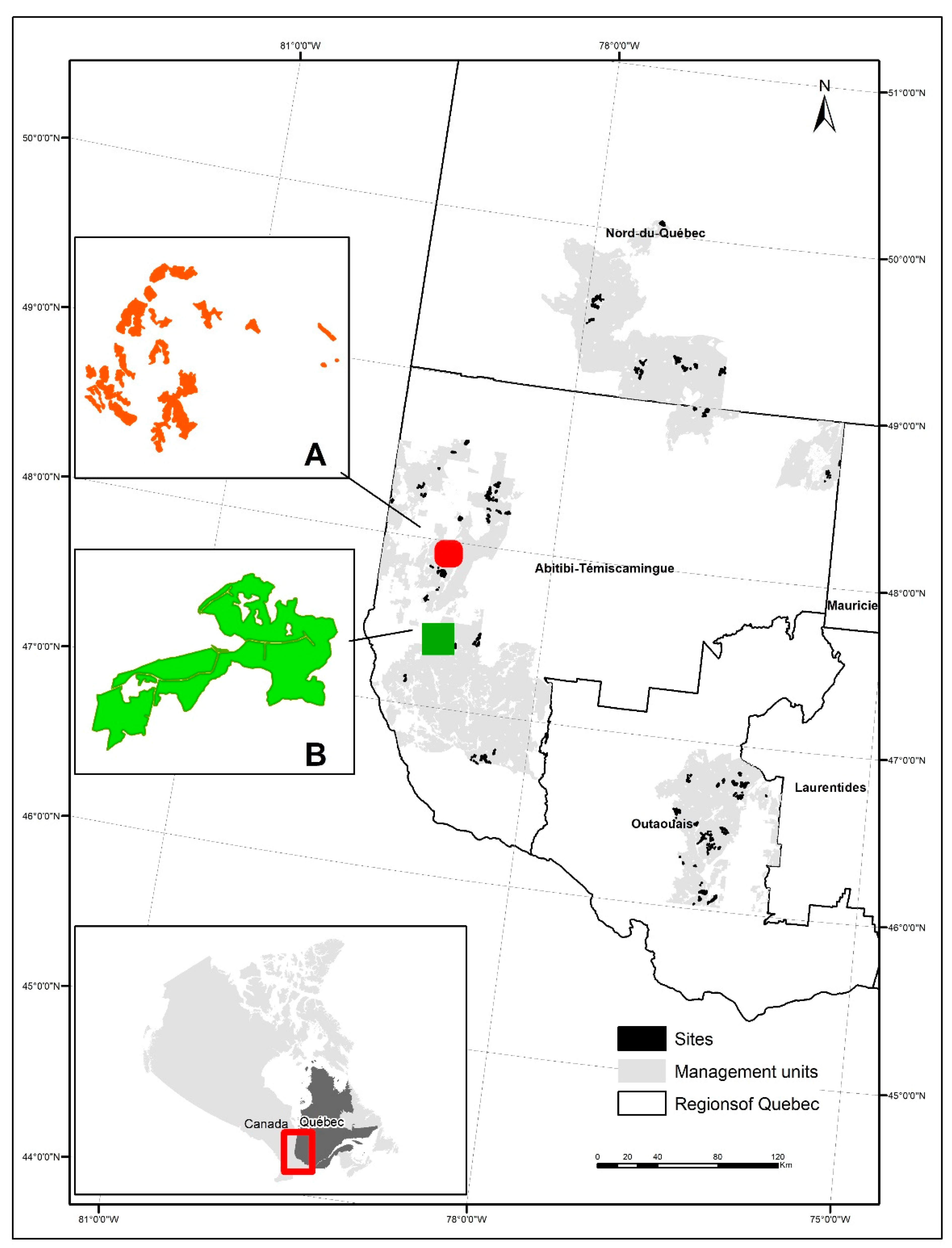
The study area encompassed different forest compositions along a north-south gradient, covering the latitudes from 46° N to 51° N. The study was located in three administrative regions of Quebec: Abitibi-Temiscamingue, Nord-du-Quebec, and Outaouais (Figure 1) and in five forest management units, which represent spatial divisions of the territory under management. Spatial and non-spatial variables were measured to describe the most representative year of activities under the tactical (5-year) plan within 50 harvested sites (hereinafter DMUs) provided by the forest minister (MFFP) be-tween 2015 and 2018 (11,159 ha). Specialized plans, such as salvage logging following natural disturbances (fires and windthrow sites) were avoided. These 50 DMUs were chosen due to the availability of initial data and to ensure that all latitudes had a minimum number of DMUs for the comparisons.
Spatial and non-spatial variables were computed for each DMU. Provincial government forestry agency data describing harvest volume and species volume potential, wood procurement costs, product values, and spatial characteristics were used to construct the database. Fourteen spatial variables (Table 1), which quantify the spatial configuration and composition of each DMU, were calculated using the spatial pattern analysis program—Fragstats version 4.2 [28]. Distance to the closest mill also was calculated, together with the total in constructed roads (km) reported for each DMU. Thirteen non-spatial variables included administration costs, harvest costs, product values, taxes, hauling costs, and the total volume harvested by species groups (conifers and broadleaf) and by type of harvest practice (clear-cut or shelterwood cut).
Figure 2 shows the distribution of some of the variables presented in Table 1. This pool of variables was our resource to choose the variables we used in the DEA analysis.
2.1. DEA Analysis
Two measures are available in the DEA. One presented by Charnes, Cooper, and Rhodes [29] that assumes a constant return to scale (CRS); for each unit increase in the inputs, a proportional increase in the outputs is generated. This measure is called aggregate or overall efficiency, which represents the ratio of potential work and actual work that is integrated into the process of wood procurement activities [30]. The second is when variable return to scale (VRS) is assumed, which means that the response of the outputs could be less than proportional (decreasing returns of scale) or greater than proportional (increasing returns of scale) [31]. This measure is called pure technical efficiency, as defined by Banker, Charnes, and Cooper [32], defined as the ability of a DMU to utilize its limited inputs to produce the desired outputs under the influence of technology and equipment. The ratio between these two efficiencies is the scale efficiency, which reflects the inefficiency due to the DMU scale of operations and size, relative unit size, or input transformations that are ineffective with respect to attaining the desired outputs [24,33].
An output-oriented DEA model was used in this study to measure the current relative efficiency level. Using available inputs, this efficiency identifies which DMU can maximize the output; in other words, which DMU can achieve a better financial outcome using current spatial organization. The free version of the spreadsheet-based software DEASOLVER LV 8.01 from Saitech Inc. (Bethesda, MD, USA), available at http://www.saitech-inc.com (accessed on 1 May 2019), was used for the efficiency assessments. This software also provides input targets for inefficient DMUs, represented as the slack of a unit when it has input excess. Slack is related to a unit’s capacity to utilize inputs in optimal proportions.
We examined homogeneity within DMUs to determine whether the following DEA assumptions were respected: (1) DMUs are engaged in the same process (forest harvesting); (2) the same inputs and outputs are applied to each DMU; and (3) DMUs are operating under the same conditions [34]. The first and second conditions were satisfied, but the third was not, given that the DMUs in the sample represented different forests, species compositions, and productivity and growth in the study area. To compensate for non-homogeneity among DMUs, the SST method proposed by Sexton, Sleeper, and Taggart [35] was used. This method incorporates regional characteristics that measure operating conditions external to the process, such as percentage of conifers or taxes, which are expected to account for efficiency differences that are not attributable to management. The SST method consists of stepwise, multiple regression on the initial efficiency scores using variables that describe the regional characteristics. Variable outputs are then adjusted using the ratio between the initial values against the predicted values, after which a second DEA is run to produce a new set of efficiency scores. These final scores focus upon the relationship between non-homogeneity and true efficiency [34,35].
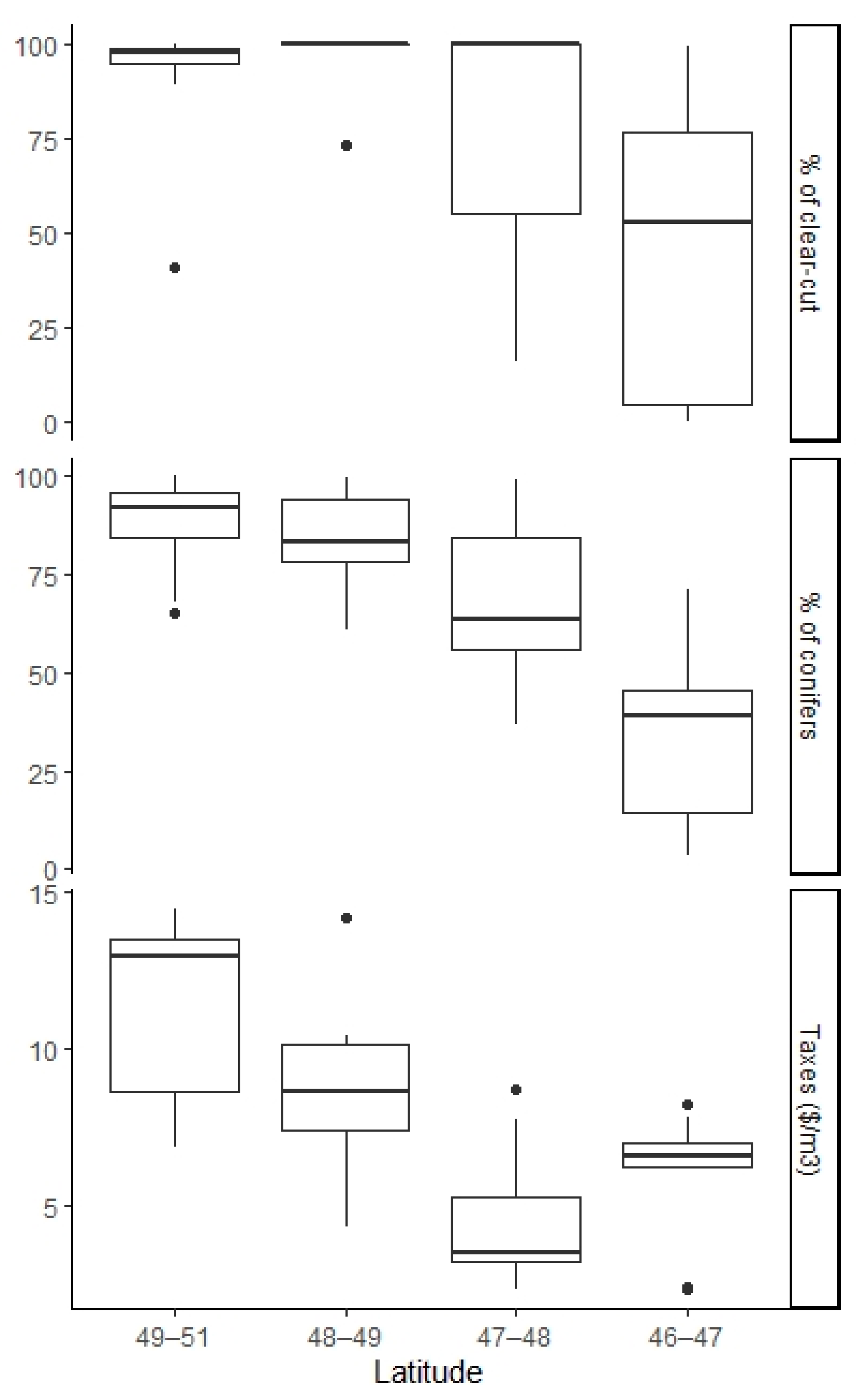
In the study area, there was a clear separation of the natural conditions of the forest and their species composition following a north-to-south latitudinal gradient. This latitudinal gradient represented an area characterized by a particular type of vegetation and reflected the balance between climate and potential vegetation. The government planned harvest activity according to the species composition of the sites [36]. Therefore, the efficiency scores were evaluated according to the latitude range of locations partitioned by 46°–47°, 47°–48°, 48°–49° and 49°–51° N.
2.2. Selection of DEA Variables
Selection of input and output variables is an important step because they are constrained by the availability and accuracy of data; the variables most have; relative independence and a minimum level of correlation with the inputs and outputs, the latter relationship’s practical meaning, and fulfilling the objectives of the study [37]. A Pearson correlation matrix (r) was constructed to eliminate redundant variables due to multicollinearity. Inputs that were correlated with the output variable were preferable due to their significant influence (over 0.3) [38]; linear regression was performed to evaluate the relationships between the inputs and outputs.
Our selected output variable for total wood procurement cost was transformed using a subtraction operation (CAD 100 less total wood procurement cost). By managing the variable in this way, we obtained a variable with positive values. DMUs with lower wood procurement costs had higher positive values for this transformed variable. Reducing costs is one of several important objectives of the forest industry, and it is also a common indicator that is often used as a performance measure leading to improved profits [27]. DEA evaluations should include the factors that globally characterize the production process; in this case, we focused on how spatial organization of the DMU affected the efficiency of financial forest activity. The variables that were included in this analysis reflected aspects related to spatial organization and wood procurement activities. We evaluated the quantity of extracted wood from each DMU and spatial distributions among patches within the DMU, which were reflected in associated road construction and the distance to the mill.
From the Pearson correlation matrix, we selected the variables that exhibited moderate correlations (|r| > 0.3) between the input and output variables [39,40]. These variables were wood volume per hectare, constructed roads, distance, LPI, and PROX CV (Table 2). The variables wood volume per hectare (X1) and wood procurement cost transformed (Y) showed the strongest correlation (r = 0.53, p = 0.0001); if the DMUs had more wood volume harvested per hectare, that would result in a higher transformed total wood procurement cost. Distance (X2) and constructed roads (X3) were moderately negatively correlated with transformed wood procurement costs; greater distance and higher road construction costs reduced the value of wood procurement costs transformed. PROX_CV (X4) and LPI (X5) also exhibited a moderately negative relationship with wood procurement costs transformed. The higher the values of PROX CV, the greater the dispersion between patches and the lower the wood procurement costs transformed will be. Based upon multiple regression, the selected variables explained 58% of the wood procurement costs transformed (adjusted R2 = 0.58, p < 0.05). The number of final variables selected and used to run the model followed the recommendation that the number of DMUs should be at least twice the number of inputs and outputs [40].
The spatial variables were evaluated with the ANOVA test to verify if they presented differences between latitudes. The results presented in Table 3 show that there were no significant differences in these variables.
2.3. Compensation for Non-Homogeneity
Before applying the SST method to compensate for non-homogeneity in the DMUs, their efficiency scores according to the latitude ranges of their locations—46°–47°, 47°–48°, 48°–49°, and 49°–51° N—were tested with the Kruskal–Wallis test, a non-parametric rank-based alternative to ANOVA [41]. The differences among the four groups were significant (p = 0.025) for aggregate efficiency (CCR), with a lower value in the north (51° to 49° N) in contrast with the other three located further south (from 49° to 46° N). For pure technical efficiency (BCC model), there were no differences among DMUs that were located at different latitudes. Differences in scale efficiency were significant (p = 0.0004) and followed the same trend as those for aggregate efficiency.
The aggregate and scale efficiency values were adjusted to compensate for the non-homogeneity prior to implementing the SST method. For adjusting the DMUs to the same conditions, environment variables that describe regional characteristics external to the process were used to explain the differences. From our initial database, the variables that differentiated the characteristics between the forests were percentage clear-cut, taxes, and percentage of conifers that presented significant differences tested with Kruskal–Wallis ANOVA across the DMU latitudinal locations. The percentage of conifers, percentage of clear-cuts, and taxes showed a gradient decreasing from north to south (Figure 3). After testing several models using these three variables, the best model that was used to correct the score for the aggregate efficiency (CCR) was a model using the percentage of harvested conifers that depended upon the availability of these species in the territory and a location variable (latitude), which explains 19% of the efficiency score (p = 0.02). The two other variables were strongly correlated with the percentage of conifers. A higher percentage of conifers permitted more clear-cutting (r = 0.66, p < 0.0001), and taxes also depended upon the quantity of conifer species that are more highly desired by industry and, hence, more valuable (r = 0.62, p < 0.0001) [42]. Because the scale efficiency is the ratio of the aggregate efficiency and the pure technique, it was recalculated with the corrected aggregate efficiency values.
3. Results
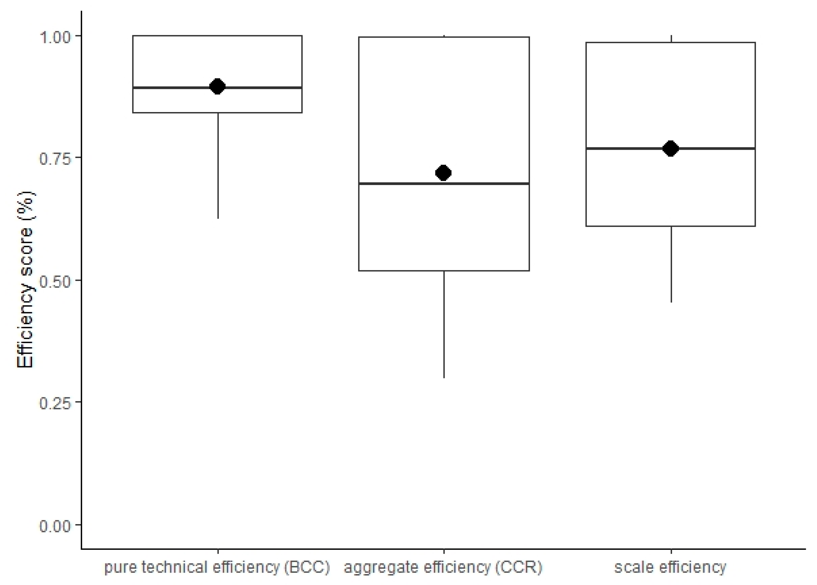
Results presented in Figure 4 summarize the mean values for the aggregate, pure technical and scale efficiencies that were calculated for the 50 DMUs in eastern Canada. They reflect efficiencies of the DMUs under the same operational conditions after integration of the compensation for non-homogeneity.
The aggregate or overall efficiency (CCR) had an average (±SD) of 72% ± 23% (median: 69%). DMUs deemed efficient (100%) totaled 13, representing 26% of the sample, while inefficient DMUs had efficiency values ranging between 97% and 30%.
For pure technical efficiency (BCC), the mean (±SD) was 89% ± 9% (median, 89%); 14 sites (28%) were considered efficient (value of 100%). This efficiency measures the extent to which DMUs could decrease the inputs to produce the desired wood procurement cost transformed, evaluating the equipment and technologies that are used in the process. Technologies included efficient machinery, combustible use, worker health, and planning strategies [43]. Scale efficiency represented the level of efficiency that is due only to the scale of operations, i.e., the relationship between aggregate and pure technical efficiency. The value of scale efficiency was 79%, with a standard deviation of 19% (median 78%); 36 of 50 DMUs were operating below optimal scales. This meant that the source of inefficiency due to the size of operations was the ability to transform the current inputs (spatial configuration of the DMUs) effectively into a lower wood procurement cost transformed.
When we differentiated efficiency values by latitudinal location, they displayed a tendency toward lower values for the DMUs that were in the northern area, with higher values for the DMUs located in the southern forests. The values for pure technical efficiency (BCC) did not differ among locations; they varied from 88% to 92%, with more variation for DMUs that were located in the south. After compensation for non-homogeneity in aggregate efficiency (CCR), the mean value for aggregate efficiency in the DMUs that were located at latitudes above 49° N was 60% (±25%) compared to the rest of the DMUs below latitude 49° N, where values ranged between 74% and 75%. Variation was greater for DMUs that were located between 47° N and 48° N (±28%), where values ranged from 100% to 29%. Finally, for scale efficiency, the DMUs located above 49° N had a mean value of 68% compared to the DMUs below 49° N, where the values were around 80%.
Figure 5 presents average target reductions for the complete set of DMUs, based upon inefficient DMUs. Targets were established using the BCC model, given that it best expressed the use of technology and managerial strategies. It was estimated that the variable distance to the mill (X2) was more efficient with lower values, 29% less than average, which equated to 41 km. Our results suggest that a 37% reduction in kilometers of constructed roads (X3) would allow optimal efficiency, equivalent to an average decrease of 2.8 km. The target reduction level for PROX_CV (X4) was a decrease of 21%. For LPI, the target was 3% on average for dominance by a bigger patch.
According to DEA results, constant returns of scale (CRS) were prevalent, with 41 DMUs operating below this scale; this demonstrated that there was no need to increase or lower the size or quantity of inputs used in the process. Three DMUs were under decreasing returns of scale; their ability to manage inputs decreased if the quantity of inputs increased. Six DMUs were observed under increasing returns to scale, where output could be maintained at the same level by increasing the scale of operations; these did not necessarily refer to the size of inputs, but to the use of more inputs (DEA model output-oriented).
4. Discussion
The results showed high values for efficiency in the harvested sites in eastern Canada. The efficiency expressed how well the current spatial configuration allowed them to maximize the financial outcome in the context of ecosystem management rules. The pure technical efficiency (BCC) averaged 89% with a low degree of variation (9%). Because this efficiency describes the intrinsic technology of the process, the high values among all the latitudinal locations studied demonstrated the advantages of the utilizing technology and management strategies, which helped reduce differences in a given territory. The overall or aggregate efficiency (CCR) was 72% (mean value); greater than 70% is considered to be good. However, this efficiency had greater variation (±23), and 74% of the DMUs (37/50) were not able to use the available inputs in transformed total wood procurement in a cost-efficient manner. The reason is that the forest industry in eastern Canada creates a year-round balance for planning for harvest sites, where access to remote sites is balanced by nearby sites to compensate for the disadvantages and extra costs of the former, and the availability of mature stands limits the possibility of operating at high efficiency everywhere. From our results, we could see both efficient and inefficient sites across the gradient of sites.
There was no significant difference in spatial variables that were evaluated for the different types of DMUs examined in the study (Table 3). Harvest areas did not exhibit a single pattern that depended upon the latitude or ecosystem in which they were located, as had been suggested by EFM. We found areas with concentrated patches dispersed along the north-south gradient, as well as small (60 ha) and large areas (400 ha). There was no tendency for areas harvested at any specific latitude to share a single pattern of spatial organization.
The spatial variables have great importance in determining the efficiency of forest harvesting at lower costs. Despite the great range of variables that were considered, those that were related to roads and to the dispersion of the patches were of greatest importance. Roads represent almost 40% of procurement costs and are essential for providing site access for timber harvesting [10,44]. From our data, road costs from construction and distance to the mill were indeed the major components of wood procurement costs. This was corroborated by LeBel and Stuart [18], who showed that hauling distance was one of the factors that explained efficiency values for contractors in the United States. Some authors from Scandinavian countries state that increasing the weight of trucks, by including high-capacity transportation (HCT) trucks in timber transport, would also bring total cost savings in roundwood transportation [45]. Road construction (km) depends directly upon the distribution and number of patches. Forest road network planning typically involves decision-making on road locations that provide access to predetermined harvesting sites in a way that minimizes overall road building and timber harvesting costs [46]. We obtained a highly significant (r = 0.57, p < 0.0001) positive correlation between the number of patches and the kilometers of constructed roads within the harvested site, and also moderate with PROX_CV and LPI (Table 2). Efficiency is affected by road construction (km), showing a direct relationship with cost. Dispersion of the patches was represented by the index PROX_CV; large values meant greater variation in the distances between patches, thereby making the areas more dispersed. Dispersion had a clear relationship with the DMUs that had the lowest efficiency values. There is evidence that aggregating harvesting areas is recognized as a means of reducing the costs of road construction and maintenance [13,47]. The large patch index showed a positive relationship with wood procurement costs; the bigger the LPI, the more efficient were the DMUs. As expected, larger areas would translate to lower wood procurement costs. In Figure 1, we present an example of the two extreme cases of DMUs. DMU1 (A) had the lowest efficiency values, with an aggregate efficiency of 48% and pure technical efficiency of 68%. The variables that described it were the number of 10 km lengths of constructed roads; the distance to the mill was 163 km, the LPI was 24%, and the PROX_CV index was 179. DMU 2 (B) had a value of 100% for both efficiencies, with a value of 2 km for length of constructed roads, distance to the mill of 60 km, an LPI of 70%, and a PROX_CV index of 31.3.
About 19% of the aggregate or overall efficiency was explained by the variable percentage of conifers when we performed the compensation of non-homogeneity with the regression of the SST method [34]. The variables taxes, clear-cut (%) and conifers (%) expressed the differences between the forest types that mainly depended on the location or latitudes where they are located. These variables help to explain the efficiency values that have been reported. Percentage of conifers that were harvested depends upon the dominant forest type and latitude, with coniferous forests dominant in the north, broadleaf forests dominant in the south, and mixed wood in-between [8]. Taxes change depending upon location according to regulations set out by the Province of Quebec, where the value depends upon the level of infrastructure in the zone and the potential species to be harvested, with higher values in areas with more conifers. The value of the taxes should be lower in the north to compensate for the operational constraints; in our sample, the values seemed to be higher, suggesting that perhaps a readjustment in tax rates is needed. Further, the percentage of clear-cut is predominant in the north, where conifers are dominant, and where the application of partial cuts is not mandatory but optional [11].
When we examined efficiencies according to different latitudes, there was a tendency toward higher efficiency values in the southern forests. However, it should be noted that efficient DMUs were present in all forest types across the range of latitudes. Southern areas may be more efficient for several reasons. First, the wood extracted has greater commercial value and larger diameters compared to the northern cuts, which is directly related to the ratio (%) of conifers at that latitude. In the North, the activity was based on extracting larger quantities of wood, but the quality of the wood was lower from trees with smaller diameters (average diameter at breast height—DBH: 16 cm; [48]) compared to trees further south (average DBH: 28 cm; [49]). Second, the road network was more developed in the south, resulting in a smaller number of roads being built; northern areas often must open new roads. Furthermore, distances to the mill tended to be shorter in the south, which made them more efficient in producing wood at a lower cost. The issue of the ratio of harvested wood volume per km of road, which affects the profitability of opening and maintaining roads [50], was less consequential in this area. Finally, higher taxes in northern areas also pose a disadvantage compared to the lower taxes in the southern areas.
We calculated two types of efficiency; the reduction in targets using aggregate efficiency (CCR) evaluates the process as a whole, which in some cases can reach 77% reduction. However, reduction targets that are based on CCR are often a result of scale inefficiency. Improvements that can be achieved through managerial means are better presented by the targets in the BCC model [24]. The goal and strategy of the forest industry is identifying the possible variables that could be important for improving the efficiency of producing wood at a lower cost [51]. From Figure 5, we can observe the improvements projected by the analysis of the variables. The main variable to improve is road construction (km); forestry roads are one of the main topics of study for the forest industry [52]. Reducing the requirement for constructed roads can be facilitated by reducing patch dispersion (PROX_CV), which has been targeted at −21%, together with the number of kilometers of roads within harvested sites. Distance to the mill directly influences the cost per kilometer of road to maintain and the cost of transport; this could be a point of improvement if there is greater coordination among contractors sharing the same territory and considering short and long term planning that will lower wood procurement costs [53]. Both targets could be addressed from the perspective of the technology if it is impossible to reduce the distance or number of kilometers to build, together with options such as vehicles that are more fuel-efficient, trucks with greater capacity, and improvements in the materials or load capacity of the roads.
Evidence regarding the nature of returns to scale in the logging industry is mixed. Here, we found that our DMUs worked under a constant return of scale (CRS), as has been mentioned by Boussofiane, Dyson, and Thanassoulis [31]. If the unit already operates in the CRS region, it usually is not a good idea to change its operating scale, given that this alteration would decrease scale efficiency. Increasing returns to scale in the logging sector have been reported by practicing foresters in a survey of contractors in New Zealand and the United States by Stuart, et al. [54]. Our study focused upon the spatial configuration of the harvested sites and not on the contractors; we presented a more general view of the process. This may explain the disparity between our results and reports in the literature.
The empirical results that are presented in this paper are an estimate of the efficiency of the harvest in Quebec according to the spatial organization and based on average and official values provided by government agencies. By no means can we claim them to be representative of the forest harvesting industry in Quebec and Canada. Some limitations of the study were the quality of available data that could be considered as a simplification of reality and may not represent the complete complexity of the regions, because some information may have been excluded from the analysis. We cannot extrapolate to regions under different conditions because the data covered only five management units of a single harvest year. The economic values that have been estimated here may not express reality because the harvested sites offered by the minister are often subject to different managerial procedures and do not necessarily follow initial limits. Additionally, the profitability may be calculated on another scale, but nevertheless, the exercise provides some insight into the advantages of this type of comparative study in forestry.
The DEA analysis allowed us to include different types of variables and to easily understand efficiency, and through the measure of target projections, how to improve performance. DEA is a relevant approach that could be more widely adopted by forest managers and government decision-makers, both locally and nationally.
5. Conclusions
In conclusion, the forest harvest evaluated at the scale of the harvested sites demonstrates the importance of spatial variables for determining efficiency values, given that they are mainly related to the dispersion of the patches, the roads that have been built, and the distance of transport from site to mill. Furthermore, we can conclude that harvested sites do not represent a single pattern that depends upon the composition of the forest in which they are found, as has been suggested by EFM directives that are currently applied in eastern Canada.
Author Contributions
Conceptualization, D.M. and O.V.; methodology, D.M. and O.V.; software, D.M.; validation, D.M.; formal analysis, D.M. and O.V.; investigation, D.M.; resources, scholarships MITACS.; data curation, D.M.; writing—original draft preparation, D.M.; writing—review and editing, O.V.; visualization, D.M. and O.V.; supervision, O.V.; project administration, O.V.; funding acquisition, O.V. Both authors have read and agreed to the published version of the manuscript.
Funding
This research was funded by Mitacs, grant number IT12691.
Conflicts of Interest
The authors declare no conflict of interest.
References
- Mobtaker, A.; Ouhimmou, M.; Rönnqvist, M.; Paquet, M. Development of an economically sustainable and balanced tactical forest management plan: A case study in Quebec. Can. J. For. Res. 2017, 48, 197–207. [Google Scholar] [CrossRef] [Green Version]
- Canada, N.R. The State of Canada’s Forests: Annual Report 2020; Government of Canada: Québec City, QC, Canada, 2020; p. 96. [Google Scholar]
- Obi, O.F.; Visser, R. Operational efficiency analysis of New Zealand timber harvesting contractors using data envelopment analysis. Int. J. For. Eng. 2017, 28, 85–93. [Google Scholar] [CrossRef]
- FAO. Natural Forest Management. Available online: http://www.fao.org/forestry/sfm/85084/en/ (accessed on 6 August 2019).
- Légis Québec. Loi Sur l’aménagement Durable du Territoire Forestier—Chapitre A-18.1. RLRQ. Available online: http://legisquebec.gouv.qc.ca/fr/ShowDoc/cs/A-18.1 (accessed on 31 December 2018).
- Gauthier, S.; Vaillancourt, M.-A.; Kneeshaw, D.; Drapeau, P.; De Grandpré, L.; Claveau, Y.; Paré, D. Une approche qui s’inpire des perturbatione naturelles: Origines et fondements. In Aménagement Écosystémique en Forêt Boréale; Presses de l’Université du Québec: Québec City, QC, Canada, 2008; pp. 15–35. [Google Scholar]
- Bergeron, Y.; Harvey, B.; Leduc, A.; Gauthier, S. Forest management guidelines based on natural disturbance dynamics: Stand-and forest-level considerations. For. Chron. 1999, 75, 49–54. [Google Scholar] [CrossRef] [Green Version]
- MRN. Le Guide Sylvicole de Québec, Les Fondements Biologiques de la Sylviculture; Ministère des Ressources Naturalles de Québec: Québec City, QC, Canada, 2013; Volume I, p. 1044. [Google Scholar]
- Baskent, E.Z.; Jordan, G.A. Characterizing spatial structure of forest landscapes. Can. J. For. Res. 1995, 25, 1830–1849. [Google Scholar] [CrossRef]
- Baskent, E.Z.; Keles, S. Spatial forest planning: A review. Ecol. Model. 2005, 188, 145–173. [Google Scholar] [CrossRef]
- Gouvernement Québec. Règlement Sur L’aménagement Durable des Forêts du Domaine de l’État. In Décret 473-2017, 10 mai 2017; Loi Sur L’aménagement Durable du Territoire Forestier (Chapitre A-18.1); Gazette Officielle du Québec: Québec City, QC, Canada, 2017; p. 62. [Google Scholar]
- Baskent, E.Z.; Jordan, G.A. Spatial wood supply simulation modelling. For. Chron. 1991, 67, 610–621. [Google Scholar] [CrossRef] [Green Version]
- Öhman, K.; Eriksson, L.O. Aggregating harvest activities in long term forest planning by minimizing harvest area perimeters. Silva Fenn. 2010, 44, 77–89. [Google Scholar] [CrossRef] [Green Version]
- Austin, R.D. Business Performance Measurement: Theory and Practice; Cambridge University Press: Cambridge, UK, 2002; p. 216. [Google Scholar]
- Gunasekaran, A.; Patel, C.; Tirtiroglu, E. Performance measures and metrics in a supply chain environment. Int. J. Oper. Prod. Manag. 2001, 21, 71–87. [Google Scholar] [CrossRef]
- Chen, N.; Qin, F.; Zhai, Y.; Cao, H.; Zhang, R.; Cao, F. Evaluation of coordinated development of forestry management efficiency and forest ecological security: A spatiotemporal empirical study based on China’s provinces. J. Clean. Prod. 2020, 260, 121042. [Google Scholar] [CrossRef]
- Homburg, C. Using data envelopment analysis to benchmark activities. Int. J. Prod. Econ. 2001, 71, 51–58. [Google Scholar] [CrossRef]
- LeBel, L.G.; Stuart, W.B. Technical Efficiency Evaluation of Logging Contractors Using a Nonparametric Model. J. For. Eng. 1998, 9, 15–24. [Google Scholar] [CrossRef]
- Drolet, S.; LeBel, L. Forest harvesting entrepreneurs, perception of their business status and its influence on performance evaluation. For. Policy Econ. 2010, 12, 287–298. [Google Scholar] [CrossRef]
- Limaei, S.M. Efficiency of Iranian forest industry based on DEA models. J. For. Res. 2013, 24, 759–765. [Google Scholar] [CrossRef]
- Salehirad, N.; Sowlati, T. Productivity and efficiency assessment of the wood industry: A review with a focus on Canada. For. Prod. J. 2006, 56, 25–32. [Google Scholar]
- Kovalčík, M. Efficiency of the Slovak forestry in comparison to other European countries: An application of Data Envelopment Analysis. Cent. Eur. For. J. 2018, 64, 46–54. [Google Scholar] [CrossRef] [Green Version]
- Li, L.; Hao, T.; Chi, T. Evaluation on China’s forestry resources efficiency based on big data. J. Clean. Prod. 2017, 142, 513–523. [Google Scholar] [CrossRef]
- Trzcianowska, M.; LeBel, L.; Beaudoin, D. Performance analysis of log yards using data envelopment analysis. Int. J. For. Eng. 2019, 30, 144–154. [Google Scholar] [CrossRef]
- Obi, O.F.; Visser, R. Influence of the operating environment on the technical efficiency of forest harvesting operations. Int. J. For. Eng. 2017, 28, 140–147. [Google Scholar] [CrossRef]
- Bonhomme, B.; LeBel, L. Harvesting contractors in northern quebec: A financial and technical performance evaluation. In Proceedings of the Forest Operations among Competing Forest Uses, Bar Harbor, ME, USA, 7–10 September 2003; p. 7. [Google Scholar]
- Hailu, A.; Veeman, T.S. Comparative analysis of efficiency and productivity growth in Canadian regional boreal logging industries. Can. J. For. Res. 2003, 33, 1653–1660. [Google Scholar] [CrossRef]
- McGarigal, K. FRAGSTATS 4.2 HELP; University of Massachusetts: Amherst, MA, USA, 2015. [Google Scholar]
- Charnes, A.; Cooper, W.W.; Rhodes, E. Measuring the efficiency of decision making units. Eur. J. Oper. Res. 1978, 2, 429–444. [Google Scholar] [CrossRef]
- Kleiner, A.; Powell, J. Jeremy Rifkin on How to Manage a Future of Abundance. Available online: www.strategy-business.com/ (accessed on 1 March 2020).
- Boussofiane, A.; Dyson, R.G.; Thanassoulis, E. Applied data envelopment analysis. Eur. J. Oper. Res. 1991, 52, 1–15. [Google Scholar] [CrossRef]
- Banker, R.D.; Charnes, A.; Cooper, W.W. Some models for estimating technical and scale inefficiencies in data envelopment analysis. Manag. Sci. 1984, 30, 1078–1092. [Google Scholar] [CrossRef] [Green Version]
- Salehirad, N.; Sowlati, T. Performance analysis of primary wood producers in British Columbia using data envelopment analysis. Can. J. For. Res. 2005, 35, 285–294. [Google Scholar] [CrossRef]
- Haas, D.A.; Murphy, F.H. Compensating for non-homogeneity in decision-making units in data envelopment analysis. Eur. J. Oper. Res. 2003, 144, 530–544. [Google Scholar] [CrossRef]
- Sexton, T.R.; Sleeper, S.; Taggart, R.E. Improving pupil transportation in North Carolina. Interfaces 1994, 24, 87–103. [Google Scholar] [CrossRef]
- MRN. The ecological land classification hierarchy. In Direction des Inventaires Forestiers; Ministere des Ressources Naturelles de la Faune et des Parcs, Ed.; Gouvernement du Québec: Québec City, QC, Canada, 2003. [Google Scholar]
- Yan, J. Spatiotemporal analysis for investment efficiency of China’s rural water conservancy based on DEA model and Malmquist productivity index model. Sustain. Comput. Inform. Syst. 2019, 21, 56–71. [Google Scholar] [CrossRef]
- Sundberg, B.; Silversides, C. Operational Efficiency in Forestry: Vol. 1: Analysis; Springer Science & Business Media: Berlin/Heidelberg, Germany, 1988; Volume 29. [Google Scholar]
- Damanik, S.E. Techniques of Efficiency Measurement in Ecology Research of Forest Management Using Data Envelopment Analysis. Int. J. Appl. Eng. Res. 2017, 12, 16024–16031. [Google Scholar]
- Kao, C.; Chang, P.l.; Hwang, S.N. Data envelopment Analysis in measuring the effieciency of forest management. J. Environ. Manag. 1993, 38, 73–83. [Google Scholar] [CrossRef]
- Vargha, A.; Delaney, H.D. The Kruskal-Wallis test and stochastic homogeneity. J. Educ. Behav. Stat. 1998, 23, 170–192. [Google Scholar] [CrossRef]
- Cayford, J. A brief overview of Canadian forestry. Unasylva 1990, 41, 44–48. [Google Scholar]
- Vanclay, J.K. Future harvest: What might forest harvesting entail 25 years hence? Scand. J. For. Res. 2011, 26, 183–186. [Google Scholar] [CrossRef]
- D’Amours, S.; Rönnqvist, M.; Weintraub, A. Using Operational Research for Supply Chain Planning in the Forest Products Industry. INFOR Inf. Syst. Oper. Res. 2008, 46, 265–281. [Google Scholar] [CrossRef]
- Korpinen, O.-J.; Aalto, M.; Venäläinen, P.; Ranta, T. Impacts of a high-capacity truck transportation system on the economy and traffic intensity of pulpwood supply in southeast Finland. Croat. J. For. Eng. J. Theory Appl. For. Eng. 2019, 40, 89–105. [Google Scholar]
- Jourgholami, M.; Abdi, E.; Chung, W. Decision making in forest road planning considering both skidding and road costs: A case study in the Hyrcanian Forest in Iran. iFor. Biogeosci. For. 2013, 6, 59. [Google Scholar] [CrossRef]
- Mathey, A.H.; Nelson, H.; Gaston, C. The economics of timber supply: Does it pay to reduce harvest levels? For. Policy Econ. 2009, 11, 491–497. [Google Scholar] [CrossRef]
- Pamerleau-Couture, E.; Krause, C.; Pothier, D.; Weiskittel, A. Effect of three partial cutting practices on stand structure and growth of residual black spruce trees in north-eastern Quebec. For. Int. J. For. Res. 2015, 88, 471–483. [Google Scholar] [CrossRef] [Green Version]
- Angers, V.A.; Messier, C.; Beaudet, M.; Leduc, A. Comparing composition and structure in old-growth and harvested (selection and diameter-limit cuts) northern hardwood stands in Quebec. For. Ecol. Manag. 2005, 217, 275–293. [Google Scholar] [CrossRef] [Green Version]
- Gharbi, C. Étude du Processus de Planification des Approvisionnements Forestiers au Québec et Mesure de sa Performance. Master’s Thesis, Univerité de Laval, Québec City, QC, Canada, 2014. [Google Scholar]
- Hansen, E.; Dibrell, C.; Down, J. Market Orientation, Strategy, and Performance in the Primary Forest Industry. For. Sci. 2006, 52, 209–220. [Google Scholar]
- FP Innovations. Forestry 4.0. Available online: https://web.fpinnovations.ca/forest-operations/forestry-4-0/ (accessed on 12 May 2020).
- Béland, M.; Beaudoin, D.; Grenier, J.-D.; Toupin, D. Optimisation des Coûts D’approvisionnement par L’utilisation des Logiciels Woodstock et FPInterface; CERFO and FP Innovations Sainte-Foy: QuébecCity, QC, Canada, 2009; p. 54. [Google Scholar]
- Stuart, W.B.; Grace, L.A.; Grala, R.K. Returns to scale in the Eastern United States logging industry. For. Policy Econ. 2010, 12, 451–456. [Google Scholar] [CrossRef]
Figure 1.
Localization of the DMUs in eastern Canadian boreal forest along a north-south gradient (46° to 50° N). Grid and regional limits (black lines). Enlarged inset areas (A,B) show examples of dispersed and agglomerated DMUs, respectively.
Figure 1.
Localization of the DMUs in eastern Canadian boreal forest along a north-south gradient (46° to 50° N). Grid and regional limits (black lines). Enlarged inset areas (A,B) show examples of dispersed and agglomerated DMUs, respectively.

Figure 2.
Box plots of some of the most representative variables for the 50 DMUs (for more details, see Table 1). The example from Figure 1 is presented showing red triangles for the dispersed DMUs (Figure 1A) and green squares for the agglomerated DMUs (Figure 1B).

Figure 3.
Boxplots of variables (% clear-cut, % conifers, and taxes $/m3) used in the adjustment of the data envelopment analysis (DEA) by latitude.
Figure 3.
Boxplots of variables (% clear-cut, % conifers, and taxes $/m3) used in the adjustment of the data envelopment analysis (DEA) by latitude.

Figure 4.
Efficiency scores of the DMUs that were examined. Black dots present the mean value.

Figure 5.
Target projected reductions for each input variable according to DEA analysis. Black dots present the mean value.
Figure 5.
Target projected reductions for each input variable according to DEA analysis. Black dots present the mean value.


Table 1.
Description of the spatial and non-spatial variables for the study area. Variables with codes prefixed by an X or Y are the ones used in the DEA analysis.
Table 1.
Description of the spatial and non-spatial variables for the study area. Variables with codes prefixed by an X or Y are the ones used in the DEA analysis.
| Variables | Description | |
|---|---|---|
| Inputs | ||
| Spatial | CODE | |
| Area Indices | AREA_MN | Mean area of harvest patches (ha) by DMU. |
| Area Total | Total area of the DMU (ha). | |
| NP | Number of patches. | |
| PD | The number of patches in 100 ha; defined as patch density. | |
| X5-LPI | Largest patch in the DMUs, expressed as a percentage and measuring dominance. | |
| Shape index | LSI | Landscape shape index, a measure of complexity and dispersion in the landscape. |
| SHAPE_MN | Average shape index of patches; measures complexity of patch shape compared to that of a square. | |
| Indices of juxtaposition and dispersion | X4-PROX_CV | Coefficient of variation of the proximity index, measures straight line-distance in radius of 500 m between patches; if the DMUs are heterogeneous, the variation is high. |
| ENN_MN | Nearest-neighbor mean (Euclidean) distance; shortest straight-line distance between patches. | |
| CONNEC | Connectivity index, the number of functional unions among patches as a percentage; 0% when it is 1 patch and 100% when all patches are connected. | |
| CONTIG_MN | Mean contiguity index, average of spatial contiguity of cells in patches. | |
| MESH | Mesh index, area of patches to reach the split level, related to index below (ha) | |
| SPLIT | Split index is the number of patches with a constant area that represent the level of separation in the landscape. | |
| Distance to mill | X2-Distance | Distance (km) between the harvest block and mill that consumes most of the wood in the zone. |
| Constructed roads | X3-Constructed road | Total graveled road construction kilometers by DMUs. |
| Non-Spatial | ||
| Bioclimatic domain | Domain | The location of the DMUs in the ecological classification reference system of Quebec |
| Volume | Volume | Total volume of harvested wood m3) |
| Type of harvest practice | % clear-cut | Proportion of clear-cut by DMUs as a percentage |
| Stand type | % Conifers | Type of dominant species in the DMUs (coniferous and broadleaf) in percentage |
| Wood volume per hectare harvest | X1-WVhh | Cubic meters of wood harvested by hectare in each DMU (average) (m3/ha) |
| Wood value | Products value | Wood product value presented in the DMUs ($/m3) |
| Taxes | Taxes | Stumpage cost for public forests ($/m3) |
| Harvested cost | Harvest cost | Cost of cubic meter by harvesting activities ($/m3) |
| Cost of roads | roads cost | Construction and maintenance cost of roads used to extract the wood during a period ($/m3) |
| Cost of transport | Transportation cost | Hauling cost by cubic meter ($/m3) |
| Profits | Profits | Financial advantage expected after reducing total wood procurement cost of wood’s values ($/m3) |
| Output | ||
| Total wood procurement cost | Total Cost | Sum of harvest cost, other cost, taxes, cost of roads and cost of transport to the mill by DMU ($/m3) |
| Transformed total wood procurement cost | Y | Wood procurement cost transformed as subtraction operation 100$—total wood procurement cost ($/m3). |
Table 2.
Pearson correlation coefficients (p-values) for inputs (X1 = WVhh (m3/ha), X2 = distance (km), X3 = constructed roads (km), X4 = PROX_CV (%), X5 = LPI (%)) and outputs Y = wood procurement cost transformed (CAD/m3) among selected DEA variables (see Table 1 for details). Bold values (p > 0.05).
| X1-WVhh | X2-Distance | X3-Constructed Road | X4-PROX_CV | X5-LPI | Y | |
|---|---|---|---|---|---|---|
| X1 | 1 | |||||
| X2 | 0.12 (0.417) | 1 | ||||
| X3 | 0.05 (0.721) | 0.06 (0.695) | 1 | |||
| X4 | 0.10 (0.493) | 0.11 (0.447) | 0.42 (0.0025) | 1 | ||
| X5 | −0.31 (0.029) | 0.01 (0.9305) | −0.35 (0.012) | −0.46 (0.0007) | 1 | |
| Y | 0.53 (0.00001) | −0.37 (0.0014) | −0.26 (0.066) | −0.17 (0.232) | −0.28 (0.048) | 1 |
Table 3.
p values from ANOVA test of the spatial variables for the locations in the different latitudes evaluated.
Table 3.
p values from ANOVA test of the spatial variables for the locations in the different latitudes evaluated.
| Variable | F Value | p Value |
|---|---|---|
| X5-LPI | 0.759 | 0.532 |
| X4-PROX_CV | 1.295 | 0.287 |
| X2-Distance | 0.622 | 0.605 |
| X3-Constructed road | 1.866 | 0.149 |
Publisher’s Note: MDPI stays neutral with regard to jurisdictional claims in published maps and institutional affiliations. |
© 2021 by the authors. Licensee MDPI, Basel, Switzerland. This article is an open access article distributed under the terms and conditions of the Creative Commons Attribution (CC BY) license (https://creativecommons.org/licenses/by/4.0/).
Share and Cite
MDPI and ACS Style
Mazo, D.; Valeria, O. Effects of Spatial Boreal Forest Harvesting Practices on Efficiency through a Benchmarking Approach in Eastern Canada. Forests 2021, 12, 1108. https://0-doi-org.brum.beds.ac.uk/10.3390/f12081108
AMA Style
Mazo D, Valeria O. Effects of Spatial Boreal Forest Harvesting Practices on Efficiency through a Benchmarking Approach in Eastern Canada. Forests. 2021; 12(8):1108. https://0-doi-org.brum.beds.ac.uk/10.3390/f12081108
Chicago/Turabian StyleMazo, Daniela, and Osvaldo Valeria. 2021. "Effects of Spatial Boreal Forest Harvesting Practices on Efficiency through a Benchmarking Approach in Eastern Canada" Forests 12, no. 8: 1108. https://0-doi-org.brum.beds.ac.uk/10.3390/f12081108
Note that from the first issue of 2016, this journal uses article numbers instead of page numbers. See further details here.