Analysis of Olive Grove Destruction by Xylella fastidiosa Bacterium on the Land Surface Temperature in Salento Detected Using Satellite Images

Abstract

Agricultural activity replaces natural vegetation with cultivated land and it is a major cause of local and global climate change. Highly specialized agricultural production leads to extensive monoculture farming with a low biodiversity that may cause low landscape resilience. This is the case on the Salento peninsula, in the Apulia Region of Italy, where the Xylella fastidiosa bacterium has caused the mass destruction of olive trees, many of them in monumental groves. The historical land cover that characterized the landscape is currently in a transition phase and can strongly affect climate conditions. This study aims to analyze how the destruction of olive groves by X. fastidiosa affects local climate change. Land surface temperature (LST) data detected by Landsat 8 and MODIS satellites are used as a proxies for microclimate mitigation ecosystem services linked to the evolution of the land cover. Moreover, recurrence quantification analysis was applied to the study of LST evolution. The results showed that olive groves are the least capable forest type for mitigating LST, but they are more capable than farmland, above all in the summer when the air temperature is the highest. The differences in the average LST from 2014 to 2020 between olive groves and farmland ranges from 2.8 °C to 0.8 °C. Furthermore, the recurrence analysis showed that X. fastidiosa was rapidly changing the LST of the olive groves into values to those of farmland, with a difference in LST reduced to less than a third from the time when the bacterium was identified in Apulia six years ago. The change generated by X. fastidiosa started in 2009 and showed more or less constant behavior after 2010 without substantial variation; therefore, this can serve as the index of a static situation, which can indicate non-recovery or non-transformation of the dying olive groves. Failure to restore the initial environmental conditions can be connected with the slow progress of the uprooting and replacing infected plants, probably due to attempts to save the historic aspect of the landscape by looking for solutions that avoid uprooting the diseased plants. This suggests that social-ecological systems have to be more responsive to phytosanitary epidemics and adapt to ecological processes, which cannot always be easily controlled, to produce more resilient landscapes and avoid unwanted transformations.

1. Introduction

Mediterranean landscapes are strongly influenced by human activities that shape the structure and functions of the landscape in consideration of human needs. Currently, the landscapes are the result of millenarian interactions between natural processes and human chose and can be defined as social-ecological systems where there is mutual evolution and adaptation between ecological processes, social, and economic components of the landscape [1,2,3,4].

In this context, the evolution of the agricultural economy has a decisive role in determining the characteristics of the landscape [5], mainly through the spatial arrangement and composition of vegetation [6,7].

Changes in land cover from agricultural activity can increase temperature on a local scale with a potential warming in deforested areas [8,9,10,11] that are connected by biogeochemical and biogeophysical processes, the latter of which influence the physical parameters that determine the availability of energy on the earth’s surface. For example, albedo alters the absorption rate of solar radiation [11].

However, the need to increase agricultural production pushes humans to replace natural vegetation with agriculture-related species, and the result is often monocultural land cover [5]. The resulting strong vegetation specialization and high social-ecological and economic connections produces a mature landscape but one that has low resilience to local disasters. Therefore, decision-makers and institutions that drive economic and social processes need to adapt their strategies and policies to influence the ability of the land to respond to disasters and stimulate the landscape regeneration [5,12,13]. This can be particularly useful following epidemic phytosanitary events that caused mass mortality.

A specific example of this critical situation is represented by the landscape of the Salento peninsula in the Apulia Region of southern Italy. It is characterized mainly by olive groves, which account for about 50% of the land cover [5,14]. Many historic trees, judging from the dimension and shape of the trunk, were declared monumental plants and are protected by Apulia regional law 14/2007.

In 2013, the phytopathogenic bacterium Xylella fastidiosa was identified in Salento [15] progressively in neighboring areas. There is also a theory in which the pathogen entered the province of Lecce in 2008–2010, but its symptoms were not immediately recognized [16]. The pathogen has had a particularly serious effect on two popular cultivars, Cellina di Nardò and Ogliarola di Lecce, which represent a substantial proportion of this widespread monoculture. The severity of the disease, coupled with the rapid spread of the bacterium, has caused and still causes unprecedented mass death of olive trees [17,18]. The event is of such magnitude that it has stimulated the research interest of the entire scientific world and the European community [19].

Therefore, X. fastidiosa is altering the land cover pattern of the landscape linked at olive groves destroying single historical olive trees as well as broad monumental olive groves at the landscape scale [20]. This change in land cover pattern linked to the agricultural landscape can devastate the provisioning ecosystem services defined as humans’ goods and services derived directly and indirectly by ecosystems and important for human well-being [20,21]. At the base of ecosystem services, ecological functions and processes are characterized by the specific land cover structures of the landscape patterns [22,23].

While the effect of X. fastidiosa on some ecosystem services, like olive groves, has been directly estimated, for others, there is no direct evidence. For example, there is little evidence about the effect of the death of olive trees on energy flow that could influence climatic change at both a regional and global scale [24,25]. In this context, we analyze the role of olive groves in microclimate regulation and the potential impact of the mass death of plants.

Land surfaces temperature (LST) from satellite images was used as a proxy variable for the effect on microclimate regulation in the main land cover types that characterize the province of Lecce. We expect that the LST time series behavior in the area of the infected olive grove if it is not appropriately managed or replaced, would over time be characterized as that of herbaceous vegetation. Therefore, a Recurrence Quantification Analysis (RQA) was performed to detect LST evolution using an ex-ante and ex-post approach to the spread of X. fastidiosa by applying a window of 18 years. The RQA is non-linear and useful for highlighting and detecting vegetation indices that show the resilience of the system at to disasters [14]. The recurrences analysis can help interpret land surface variation on a provincial scale to show the cumulative effect of X. fastidiosa on the olive groves, highlight its potential start, and show the human response to the epidemic.

2. Materials and Methods

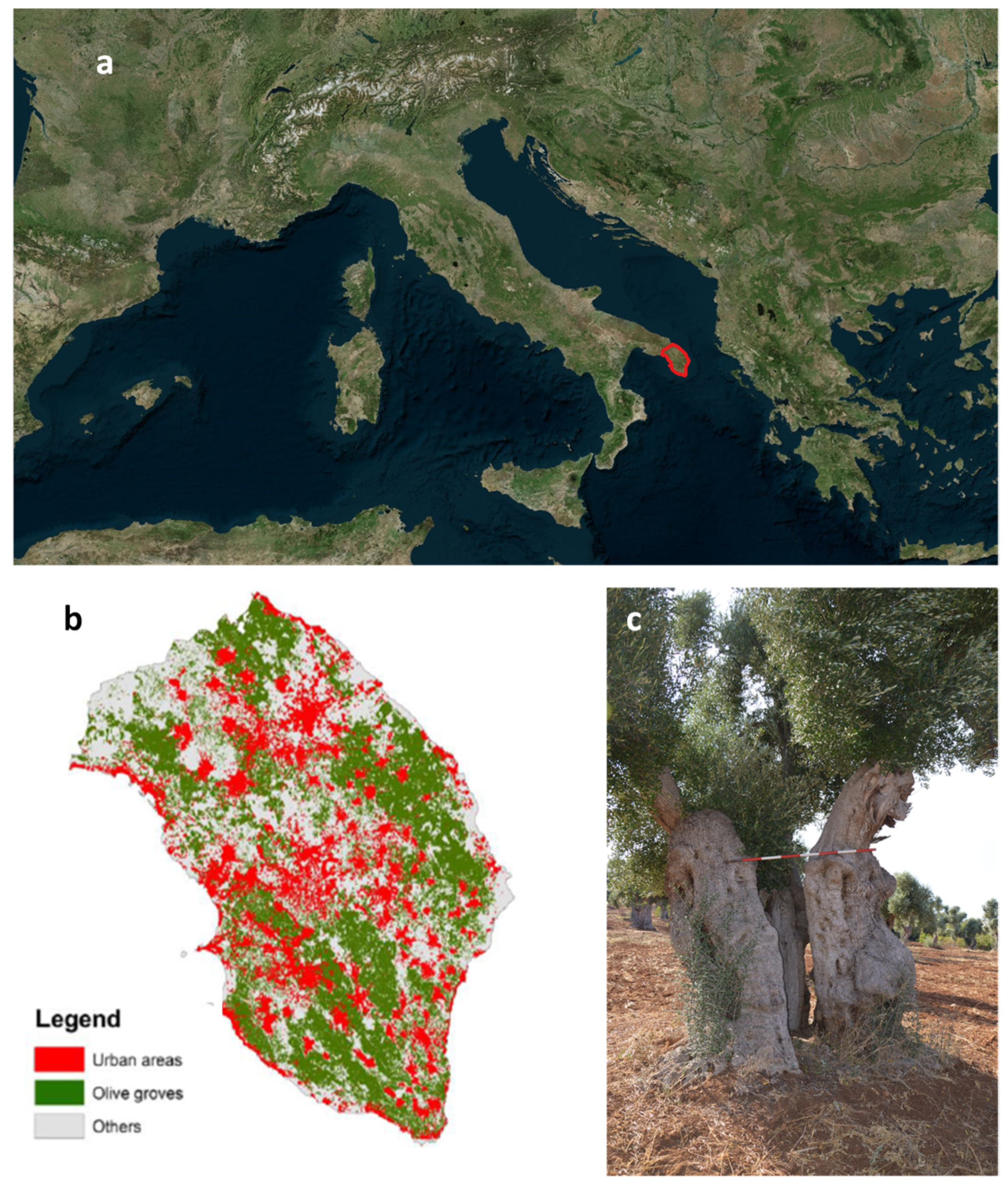
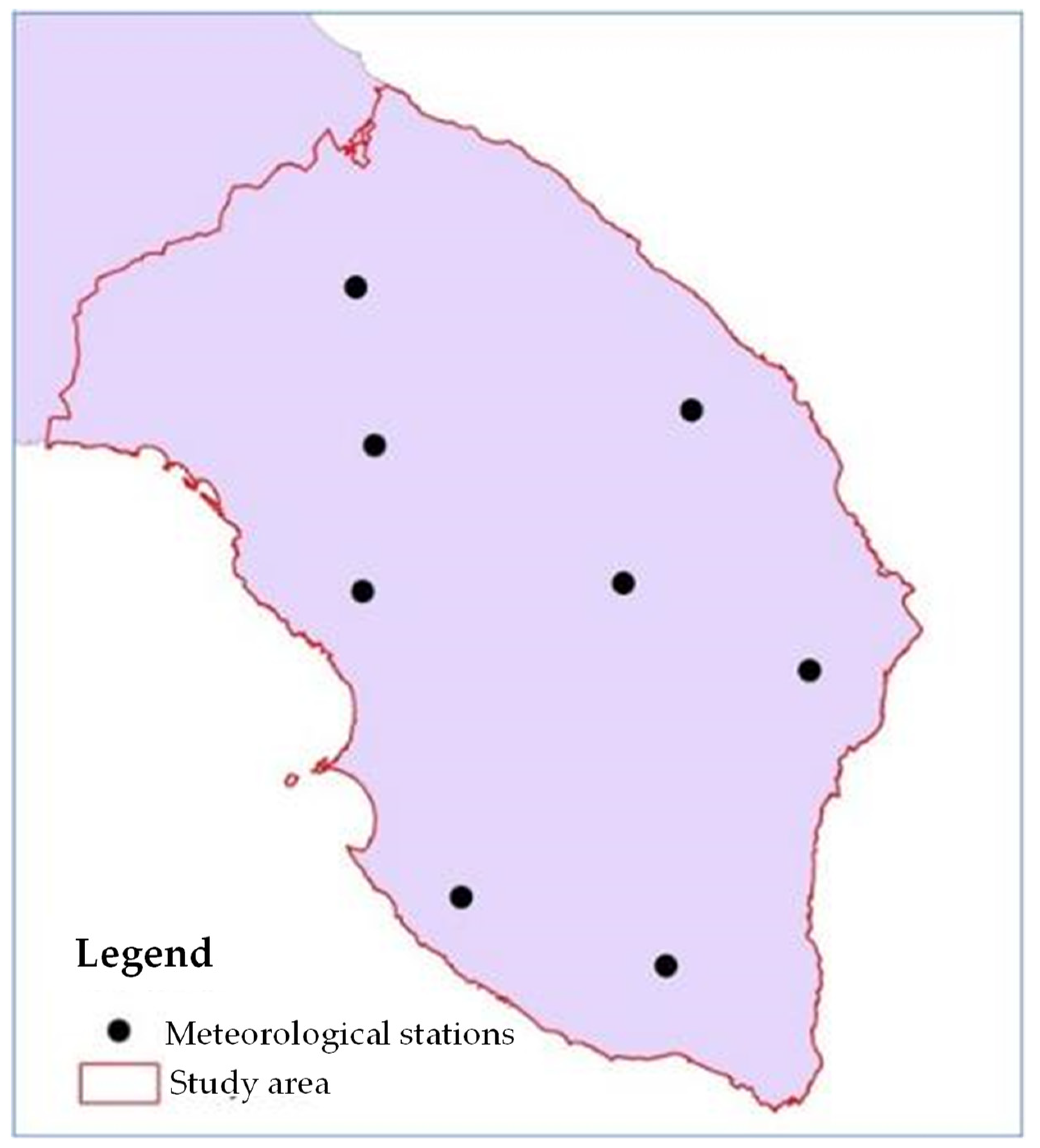
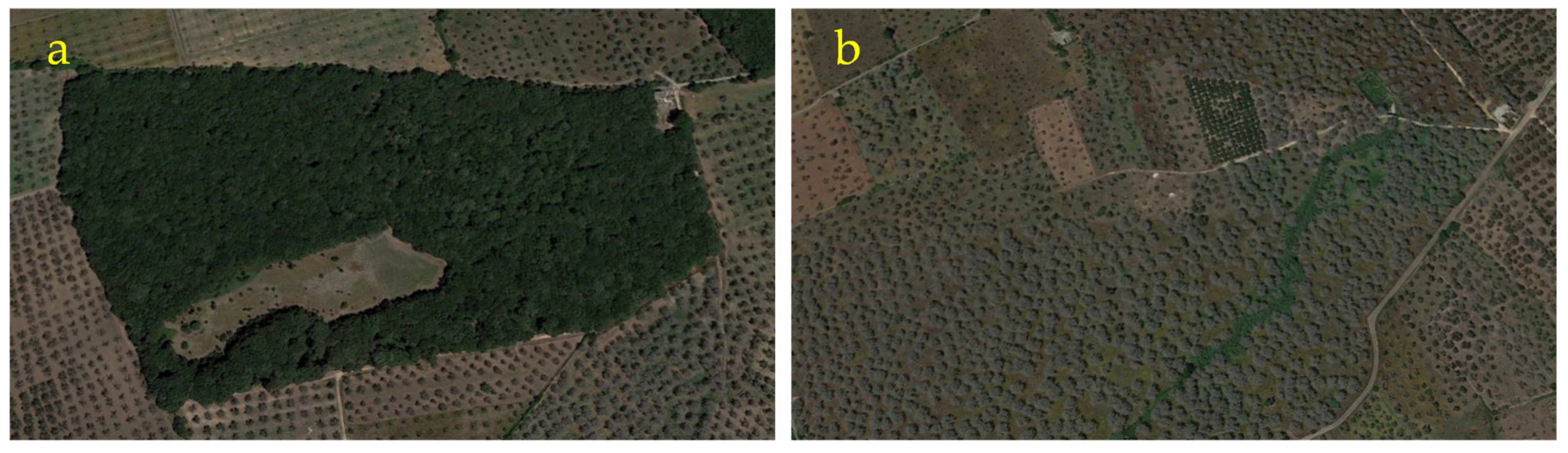
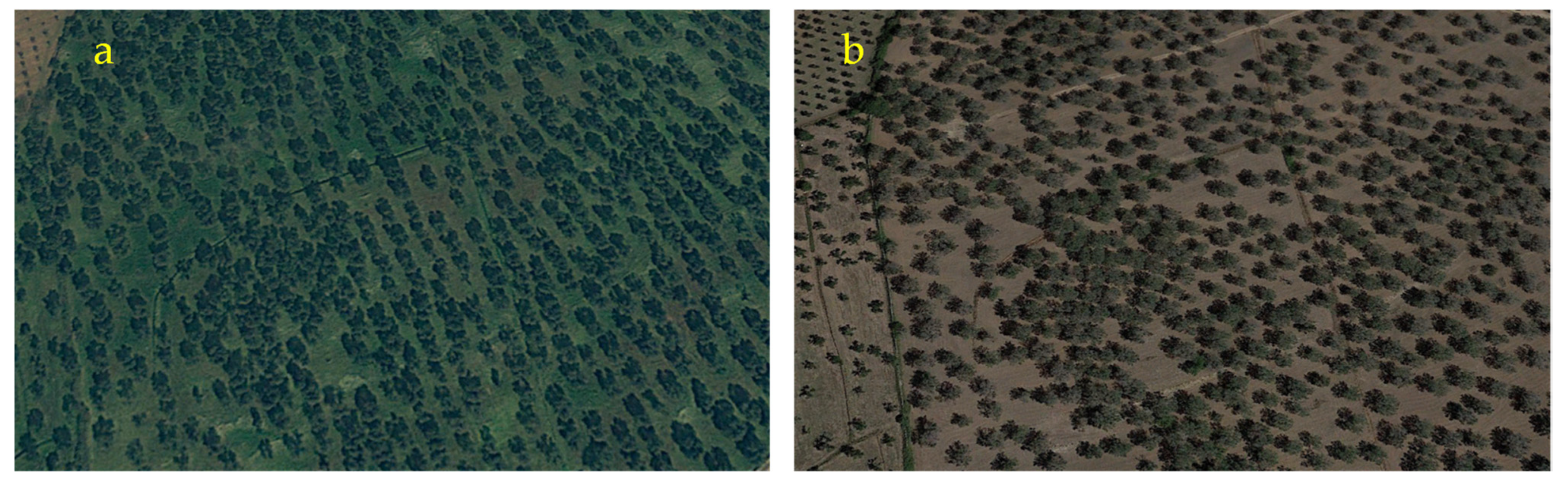
2.1. Study Area

An LST analysis of the agro-ecosystem that characterizes the Salento Peninsula in the Apulia region of southern Italy was performed [5] (Figure 1).

The agro-ecosystem is characterized mainly by olive groves, farmland and vineyards. Natural vegetation is characterized by isolated forested nuclei, grass and small wetlands [26]. At present, the whole province of Lecce is declared to be an X. fastidiosa infected area (Commission Implementing Regulation (EU) 2020/1201).

2.2. Satellite Data

The study was carried out using Landsat 8 data and Moderate Resolution Imaging Spectroradiometer (MODIS) images provided by the National Aeronautics and Space Administration (NASA) and the U.S. Geological Survey (USGS) [27,28]. Data were analysed using the QGIS, Octave and Matlab software.

Band 4, Band 5 (with spatial resolution of 30 m) and Band 10 (spatial resolution of 100 m) from Landsat 8 were used to analyze LST variation in the spring and summer from 2014 to 2020 [29,30].

The MOD11A2 product was used to build the LST temporal profile from 2003 to 2020 with a 1 km spatial resolution and an 8-day time step [31].

Land cover from the Apulia Territorial Information System (SIT Puglia) for 2011 was used to build a Region of Interests (RoI) and extrapolate LST data for olive groves, farmland, vineyards and forest [32]. Furthermore, to evaluate the effect of climate conditions on the satellite data, we used air temperature and precipitation data provided by Civil Protection of the Apulia region [33].

2.3. Analysis of LST Landsat 8 Data for Land-Cover Types

The LST for olive groves, farmland, vineyards and forest was calculated for the spring and summer from 2014 to 2020, one year after official pathogen detection (2013). Landsat 8 images from 1 March to 10 May (for the springtime) and from 21 July to 11 August (for the summertime) were used. For each time window, only images with high quality and low cloud cover were selected.

For this analysis, Band 10 (thermal infrared) was converted in Brightness Temperature, while band 4 (red) and band 5 (infrared) were useful for determining the Normalized Difference Vegetation Index (NDVI) [29,30,34,35] as follows:

$$\mathrm{NDVI}=\frac{\left(Band5-band4\right)}{\left(Band5+band4\right)}$$

(1)

The index was used to estimate the land cover emissivity (

Table 1. Standard values of emissivities used in the LST analysis (Jeevalakshmi et al., 2017).

NDVI Range	Emissivity Value (ԑ)	Land-Cover Type
NDVI ≤0	0.991	Water
0 < NDVI < 0.2	0.966	Soil
0.2 ≤ NDVI ≤ 0.5	Applied Equation (2)	Mixture of soil and vegetation cover
NDVI > 0.5	0.973	Natural vegetation (forest or wetland)

). For an NDVI in the range of 0.2–0.5 the emissivity was calculated using the following equation [29,30].

$$\mathsf{\epsilon }={\mathsf{\epsilon }}_{\mathrm{v}}\times {\left(\frac{NDVI-NDVIs}{NDVIv+NDVIs}\right)}^2+{\mathsf{\epsilon }}_{\mathrm{s}}\times [1-{\left(\frac{NDVI-NDVIs}{NDVIv+NDVIs}\right)}^2]+\mathrm{C}$$

(2)

where ԑ_v and ԑ_s are the land cover emissivity and C is the surface roughness (considered with an uniform value of 0.005 [30,36].

The LST was calculated using the following equation [29,30,37]:

$$\mathrm{LST}=\frac{\mathrm{BT}}{\left\{1+10.8(BT|14388)\ast \ln \left(\mathsf{\epsilon }\right)\right\}}$$

(3)

where BT is the brightness temperature.

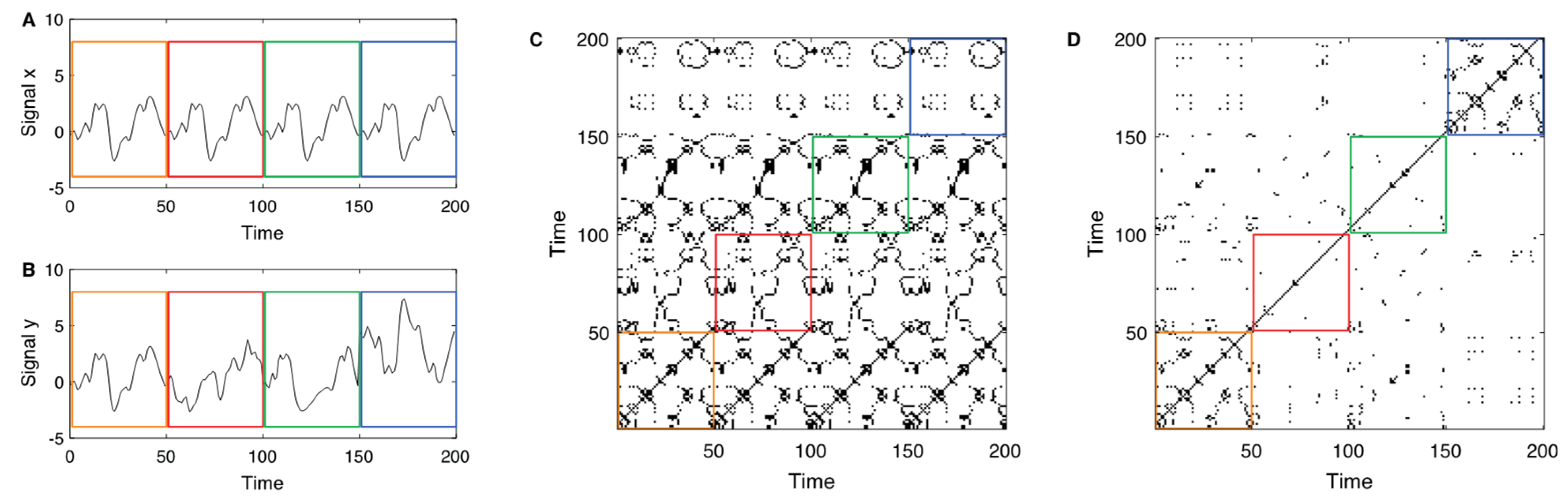
2.4. Recurrence Analysis of LST Time-Series Using MODIS Data

To analyze the climate effect of X. fastidiosa and the potential evolution of regional plans and policies, LST time series from 2013 to 2020 were built for farmland and olive groves using the MOD11A2. Here, we studied their relationship by comparing their their recurrence structure.

Each land cover is characterized by the periodic recurrence of vegetative states over a season influenced by climate conditions, such as periodic recurrences caused by the seasonal effect in the vegetation time series [20]. This recurrence state can change in time as a consequence of disturbing events and can be investigated by the recurrence analysis [38].

A recurrence structure change can be highlighted using recurrence plots (RPs), which indicate all pairs of time points (i, j) where the system recurred to a preceding state x_i [39,40]:

R_{i, j} = θ(ε − ‖x_i − x_j‖)

(4)

The recurrence matrix R consists of a characteristic pattern and can be considered as a fingerprint of the dynamics represented by the time series. The Cross Recurrence Plot (CRP) highlights the co-occurrence of similar states of two time series, whereas the Joint Recurrence Plot (JRP) highlights the simultaneous occurrence of recurrences between two time series [14,39,40]. The CRP between the variables $x_i$ and $y_i$ is determined by:

C_{i, j} = θ(ε − ‖x_i − y_j‖)

(5)

and the JRP is determined by the RPs multiplication of each system $x_i$ and $y_i$:

J_i,j = θ(ε_x − ‖x_i −x_j‖) × θ(ε_y − ‖y_i − y_j‖)

(6)

where $x_i,y_i\in R$ represents the farmland and olive grove LST time series, respectively; I, j = 1,….N; N is $x_i,y_i$; time series length ε is a threshold distance; θ(•) is the Heaviside function and ‖•‖is a norm [14,39].

In the CRP, the main measure of similarity is represented by the Line of Synchronization (LoS). For two equal signals, the LoS corresponds to a continuous line in the main diagonal in the plot, whereas deviations between two signals correspond to interruptions, or bendings, of the LoS (Figure 2A–C). Instead, the LoS completely vanishes for completely different signals. The LOS is useful for studying synchronization or time distortions [41].

Therefore, for the synchronization analysis, the F-recurrence measure defined for the CRP was used. It is given by $\frac{1}{N}{{\displaystyle \sum }}_i{C}_{i,i}$, which quantifies the density of points along the main diagonal. The F-recurrence measure is 1 for total synchronization and tends to very small numbers for highly desynchronized systems [14].

The JRP is always a main diagonal because it is based on individual RP signals. Here, the analysis is carried out by calculating the recurrence points loss in the JRP with respect to the individual RPs. In two signals with the same recurrence pattern, the JRP corresponds to individual RPs because each same recurrence point between two RPs is preserved in the JRP, whereas specific deviations between the two signals in individual RPs can produce a corresponding loss of recurrence point in the JRP. This allows checking for generalized synchronization (Figure 2A,B,D) [14].

The diagonal lines in JRP indicate that the two variables have states that repeat at the same time (each variable recurred at the same time) and therefore the variable presents a similar evolution. Determinism Det = $\frac{{{\displaystyle \sum }}_{lmin}^{N}lP\left(l\right)}{{{\displaystyle \sum }}_{l=1}^{N}lp\left(l\right)}$ is a measure that quantifies the fraction of recurrence points that form the diagonal lines in the JRP with P(l) the histogram of lengths of such diagonal lines [40,41,42].

The CRP and JRP analysis was combined with a sliding window approach to detect the temporal effect of X. fastidiosa in LST time series evolution and synchronization. For CRP, overlapping was applied, and a sliding temporal windows with a “one-year length” to the LST time series was used to calculate the Det and F-recurrence parameters ex-ante and ex-post the X. fastidiosa spread in consideration of the assumption that it may have been introduced earlier than 2013 [14,16]. For the recurrence threshold, an empirically defined threshold was used to ensure a fixed number of recurrence points (measured by recurrence rate, $RR=\frac{1}{N}{{\displaystyle \sum }}_{i,j=1}^N{R}_{i,i}$ of $Fixed RR=0.2$). The selected value did not qualitatively affect the used recurrence measures because of its low qualitative effect in this and similar studies [14,40,41]. The RQA was performed with “CRP Toolbox” in MATLAB software (http://tocsy.pik-potsdam.de/CRPtoolbox/ accessed on 15 June 2021).

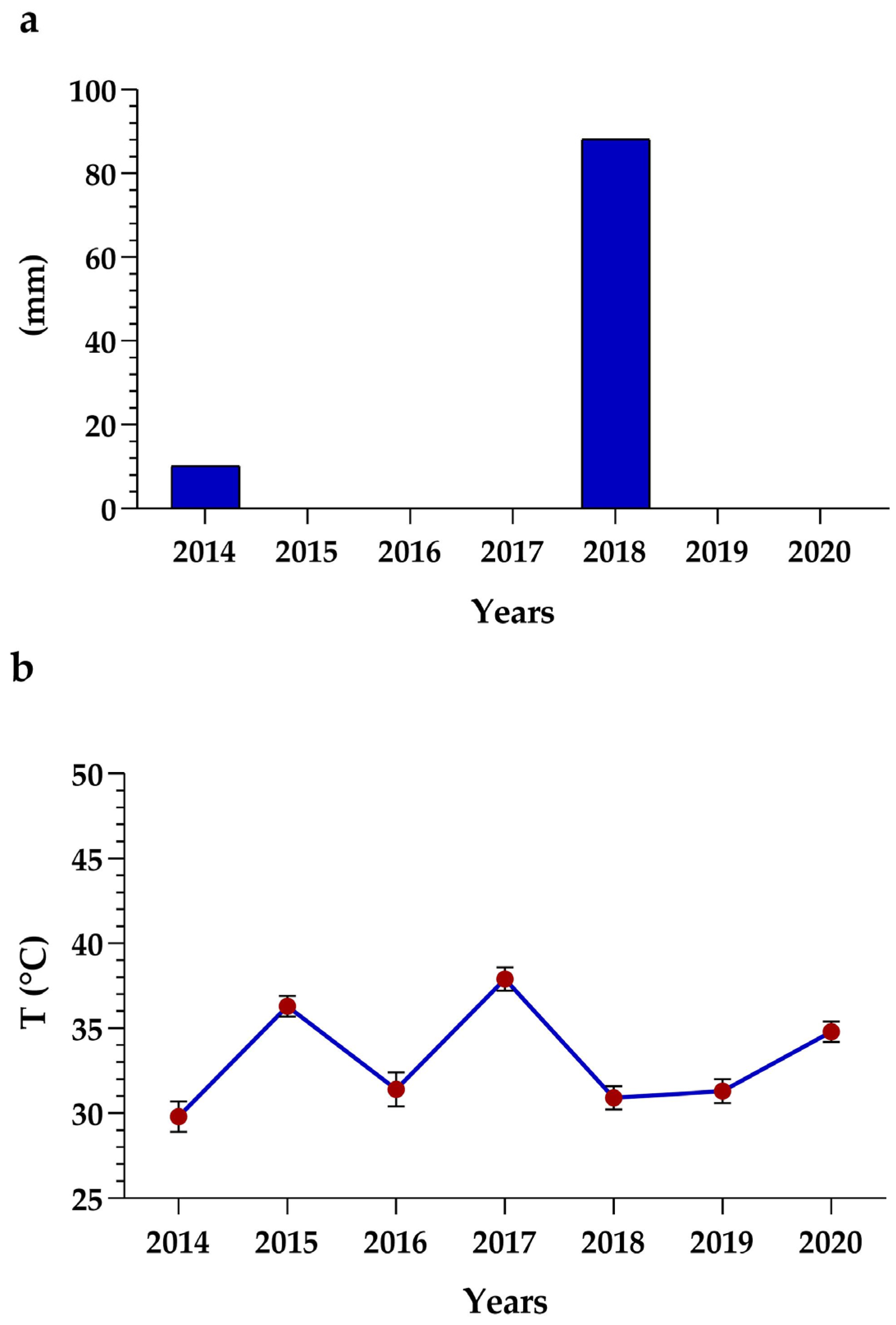
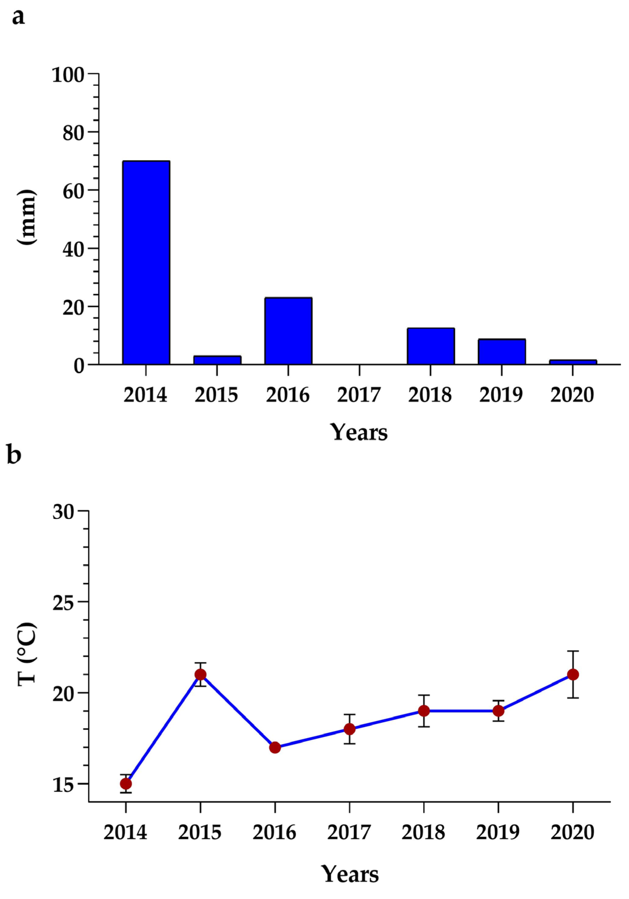
2.5. Analysis of Climate Data

Since the LST can be affected by meteorological conditions, data for each Landsat image came from 8 meteorological stations managed by the Apulian Civil Protection [33] (Figure 3). Specifically, the air temperature for six days before image acquisition was considered and the average value was calculated. Moreover, for the same period, the cumulate precipitation was also acquired.

3. Results

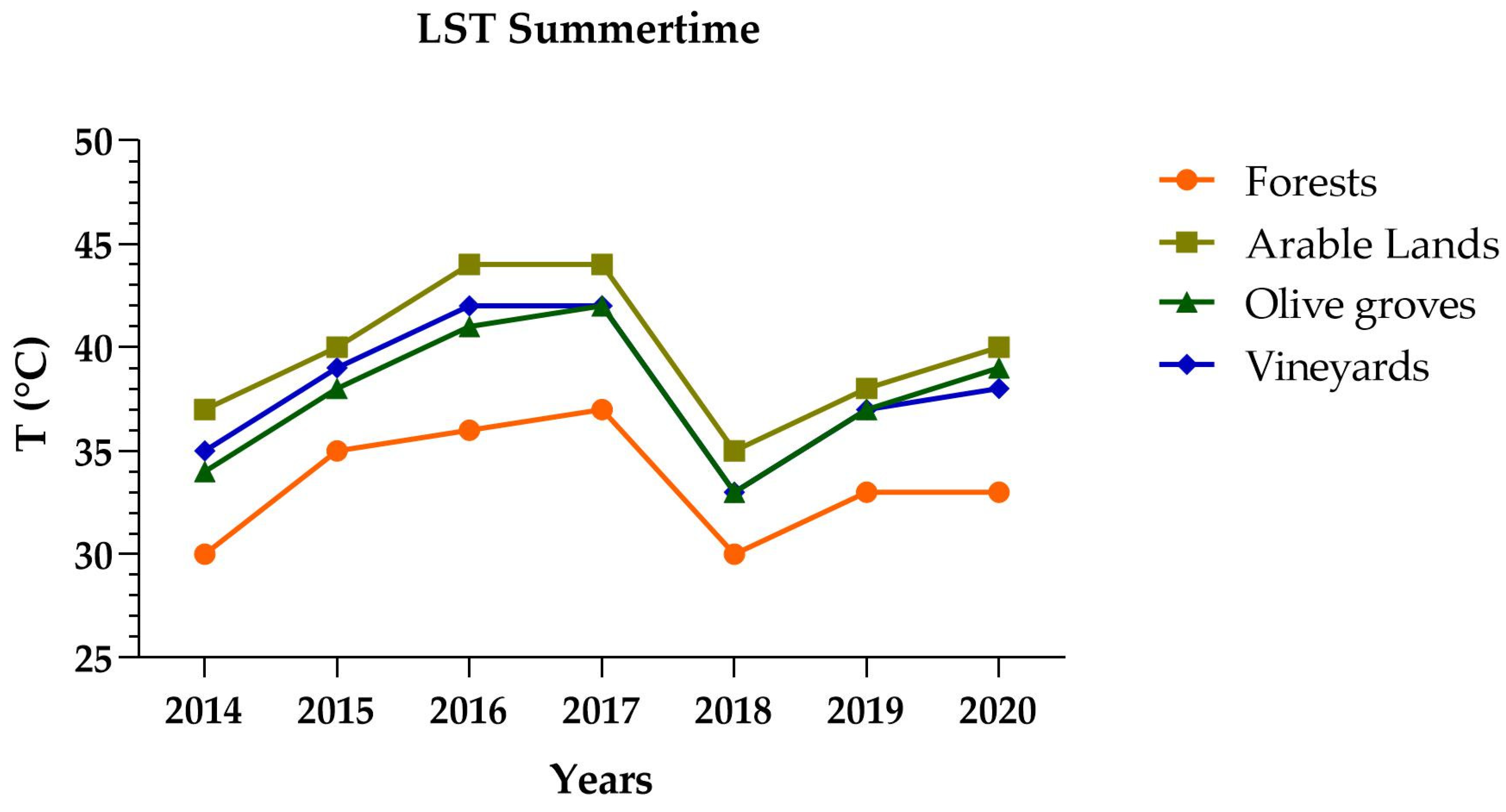
3.1. LST Landsat 8 Analysis

The analysis of average LST values in summer for different land cover types showed that forests had a high capacity for reducing LST while farmland had the lowest (Figure 4). The olive groves and vineyards showed average values of the LST; from 2014 to 2016, the LST of the olive groves was lower than vineyards, while from 2017 to 2020, it was higher.

As reported, the LST value is influenced by climate conditions: the low value of LST for 2014 and 2018 corresponds to a high value of cumulative precipitation and low air temperature, while the highest value for the year 2017 corresponds to the absence of precipitation and the highest air temperature (Figure 5). The Fisher test showed that the average LST for different land cover types for different years belonged to distributions having a different variance (

Table 2. Fisher test and Student test to analyse the statistical differences among the land covers reported in the Figure 4.

Years	O-A		O-F		O-V		A-F		A-V		F-V
	α = 5%		α = 5%		α = 5%		α = 5%		α = 5%		α = 5%
	Ftab = 1.01	Ttab = 1.65	Ftab = 1.01	Ttab = 1.65	Ftab = 1.01	Ttab = 1.65	Ftab = 1.01	Ttab = 1.65	Ftab = 1.01	Ttab = 1.65	Ftab = 1.01	Ttab = 1.65
	F-Test	t-Test	F-Test	t-Test	F-Test	t-Test	F-Test	t-Test	F-Test	t-Test	F-Test	t-Test
2014	1.385	406.902	1.806	279.342	1.140	99.681	1.304	394.615	1.579	166.853	2.059	290.473
2015	1.119	418.556	2.604	273.148	1.520	143.660	2.328	412.609	1.700	143.995	3.958	304.558
2016	1.161	478.017	2.240	388.510	1.207	76.147	1.930	539.160	1.401	237.241	2.704	360.905
2017	1.607	393.575	3.532	483.039	1.108	87.044	2.198	519.295	1.450	298.324	3.188	306.241
2018	1.156	298.964	1.189	231.560	1.813	18.900	1.374	374.642	1.568	231.429	2.155	226.394
2019	1.152	142.507	2.382	333.169	1.446	99.207	2.067	354.766	1.666	182.318	3.443	230.991
2020	1.126	180.511	2.137	487.116	1.455	114.136	1.898	514.249	1.638	222.178	3.109	362.063

), while the average values of the Student’s t test were statistically different. Indeed, in the tests the values were higher than the references tabulated to determine the significance.

The analysis of average values of LST in the spring for different land cover types shows that the forest land cover always had the highest ability to reduce LST, while the vineyards had the lowest (Figure 6).

The olive groves and farmland had close average LST values. In general, the differences were less pronounced than in the summer. The Fisher test showed that the average LST for different land cover types for the different years belong to distributions with different variance (

Table 3. Fisher test and Student test to analyse the statistical differences among the land covers reported in Figure 6.

Years	O-A		O-F		O-V		A-F		A-V		F-V
	α = 5%		α = 5%		α = 5%		α = 5%		α = 5%		α = 5%
	Ftab = 1.01	Ttab = 1.65	Ftab = 1.01	Ttab = 1.65	Ftab = 1.01	Ttab = 1.65	Ftab = 1.01	Ttab = 1.65	Ftab = 1.01	Ttab = 1.65	Ftab = 1.01	Ttab = 1.65
	F-Test	t-Test	F-Test	t-Test	F-Test	t-Test	F-Test	t-Test	F-Test	t-Test	F-Test	t-Test
2014	1.240	208.260	1.169	51.722	1.004	214.159	1.061	132.766	1.236	57.069	1.165	167.513
2015	1.659	5.193	1.131	282.100	1.962	207.320	1.876	216.525	1.183	162.384	2.219	294.208
2016	2.534	114.628	1.333	53.919	1.433	261.573	3.378	76.085	1.769	108.880	1.910	185.564
2017	1.066	99.611	1.070	98.618	1.026	150.788	1.141	143.301	1.040	80.391	1.097	175.149
2018	1.909	13.458	1.206	247.566	2.406	184.654	1.629	172.361	1.225	141.003	1.995	236.795
2019	1.041	148.201	1.089	124.289	1.185	44.067	1.046	183.474	1.233	55.436	1.290	141.247
2020	1.703	54.835	2.463	278.256	1.636	177.178	1.446	233.004	1.041	104.748	1.506	268.300

), while the average values for the Student’s t test were statistically different. Indeed, in the tests the values were higher than the references tabulated to determine significance.

In this case, the LST values seem to be mainly influenced by air temperature as high values of air temperature correspond to high values of LST and vice-versa (Figure 7).

3.2. Recurrence Quantification Analysis of LST Time Series

To better analyze the impact of X. fastidiosa on the LST evolution of olive groves, the JRP between olive grove and farmland LSTs was carried out from 2003 to 2020, using a four-year sliding temporal windows. For each time window, the Det parameter was estimated.

The JRP-based measure identified a shift in the generalized synchronization around 2009–2010. This shift could be interpreted as the evolution of olive grove land surface temperature to one of farmland (Figure 8).

The synchronization between farmland and olive grove LSTs was evaluated using a one-year sliding temporal windows on CRP before and after the spread of X. fastidiosa. The F-recurrence was calculated in each time step for the two LSTs.

The analysis revealed a pretty small value for the F-recurrences, i.e., the farmland and olive groves LSTs were only weakly related. Moreover, this weak interrelationship did not change over time, as shown by very similar values for the F-recurrences. According to the F-test, there is no statistically significant difference in the distribution of the F-recurrence between the ex-ante and ex-post 2010 time. The p-values of the F-test was 5% higher than the threshold (

Table 4. Statistical analysis on the F-recurrence distribution ex-ante and ex-post 2010.

F-Recurrence	Mean	Std. Dev.	F_b-a	Ftab	Alpha
LST-before	0.207	0.199	1.08	1.41	p > 0.05
LST-after	0.208	0.207

), so we could not reject the null hypothesis that the mean values for the F-recurrence distribution before and after the trigger event were referenced at distribution values with a similar variance. This suggests that X. fastidiosa did not have effect on the pattern synchronization of the variables.

4. Discussion

The LST Landsat images showed that the olive groves did not have the same ability as the forest to mitigate the rise in temperature; indeed, in both times the olive grove LST was higher than the forest LST. This difference was accentuated in the summer and could have been influenced by the differences in their respective canopy structures. Therefore, even if many groves were characterized by monumental plants with trunk diameters greater than 80 cm, the canopy structure was less dense than that of forests, which could explain the low ability to regulate the microclimate of the ecosystem (Figure 9).

Furthermore, the LST of the olive groves was influenced by background vegetation, which are grassland or bare soil considering the agriculture practices in spring and summer (Figure 10). Indeed, we observed some similarity between olive groves and farmland in the spring and with vineyards in the summer. This was confirmed by the F-recurrence parameter between olive grove and farmland LSTs before and after 2010 that showed that these land cover types had the same synchronization independent of the spread of X. fastidiosa.

The Landsat analysis did not show any direct effect of X. fastidiosa on LST even though a drastic increase in olive grove LST from 2014 to 2020 was expected as a consequence of the death of olive trees mainly of the monumental trees. This is because the bacterium diffusion presumably started some years before the 2013 detection but achieved maximum diffusion and effect later, forcing the Apulia region to declare the study area compromised. The meteorological conditions during image acquisition had a strong effect on LSTs. In any case, this was also influenced by different factors. First, infected and dead olive trees remained in the field for a long time because cutting operations only began in recent years. Second, dying plants still developed basal suckers with leaves, which shaded the soil affecting LST values (Figure 11).

However, in the summer of 2019 and 2020, the LST of the olive groves was near the value recorded for farmland, whereas it was lower than for vineyards from 2014 to 2016, and the highest values from 2017 to 2020. This could be connected to the low canopy structures of the olive groves which had a major effect in the evolution to a farmland LST.

The evolution of the olive grove LST into a farmland LST because of X. fastidiosa diffusion was confirmed by the Det profile of JRP, which showed an increase after 2010. This seemed to support the argument that X. fastidiosa was introduced before 2013 [16]. The substantial variation of Det in behavior before 2010 can be linked to cultivation practices like olive tree pruning. On the other hand, the Det analysis after 2010 showed a more or less constant behavior without substantial variation; therefore, this can be the index of a static situation in the evolution of this system. It does not indicate a recovery or transformation for the dying olive groves.

The olive groves can have effects in provide microclimate mitigation ecosystem services in the agroecosystem landscape, which are important in the summertime where the air temperatures have the highest values. For example,

Table 5. Land Surface Temperature differences between olive groves and farmland from 2014 to 2020.

Years	LST Difference between Farmland and Olive Groves (°C)
2014	2.8
2015	2.2
2016	3.0
2017	2.0
2018	1.8
2019	0.8
2020	0.9

shows how the average LST from 2014 to 2020 between olive groves and farmland ranged from 2.8 °C to 0.8 °C. These differences can affect the rural landscape where there is a strong interaction between urban sprawl and olive groves (Figure 12).

This study was carried out at a provincial scale; therefore, it can describe general situations but specific analysis at a smaller scale is needed for a specific context, such as the interface between urban areas and olive groves or where the isolated urban settlements extend into olive groves [43].

Indeed, a limitation of the study was the spatial resolution of satellite images considering the fragmentation of the landscape. Therefore, it was not possible to apply the Recurrence Quantification Analysis to forests and vineyards due to the small size of the patch in these land cover types and the poor spatial resolution (1 km) of the MODIS data for LST. The results reported here are in accordance with the literature, indicating that RQA analysis applied at remote sensing vegetation indices and other parameters is an efficient approach for analyzing the connection between climate systems and environmental variables over extensive areas [14,44,45,46,47]. Moreover, these findings show the usefulness of analyzing the response of a landscape system to a specific disaster or to highlight the evolution of a system into a new configuration [14,44,45,46,47].

The Vision of Recurrence Analysis in Panarchy Approach

X. fastidiosa produced a fast change in the landscape, destroying a historical agro-ecosystem that had been developed over centuries. Moreover, the analysis showed how ecological processes act independently and unpredictably. At the same time, the social and economic components of the social-ecological system showed low resilience and a slow adaptative ability to respond adequately to a disaster.

The JRP analysis showed a static evolution of affected olive groves areas and if the institutional components had developed policies to replant olive trees or reproduce a similar canopy structure using different woody plants. Therefore, this can be considered the example of a panarchy effect where the staticity can be corresponding at the slow capacity of social and institutional components to develop adaptative strategies at such fast perturbations actions generated at the landscape scale. For this reason, decision-makers must act with greater incisiveness and take more effective actions to tackle the environmental problem created by X. fastidiosa (Figure 13).

Resistance to uprooting the infected monumental trees at the outset of the X. fastidiosa diffusion was linked to historical landscape conservation and may have slowed down landscape regeneration. We cannot say whether a more timely uprooting of the infected plants (as well as insect vector control) could have reduced the spread of the disease, but replacing them with new plants (resistant to the pathogen or non-host plants) would have helped develop new olive vegetation by accelerating the resilience mitigation of the local microclimate and others not studied here, but which are directly connected with the olive culture and the production of extra virgin olive oil.

5. Conclusions

In this study, remote sensing data was useful for analyze the Xylella fastidiosa effect in a retrospective way and in the province of Lecce (South Italy), where in situ field variable measurement is not available. This type of analysis is useful for predicting the landscape evolution and ecological processes on a local scale. Furthermore, the study highlighted how nature responded faster than humans to the bacterial invasion. For the aim of the study, the JRP was more relevant than CRP for analyzing the differences caused by X. fastidiosa, possibly because the CRP was influenced by the breakpoint choice. Therefore, the JRP showed a strong ability to study the evolution of the system in a non-linear way to monitor the X. fastidiosa pathogen in a way that was less influenced by the setting of the analysis or without knowing the precise time when it occurred.

The destruction of the monumental olive groves in the province of Lecce was not only an agricultural and economic disaster that had a negative effect on the aesthetics of the landscape, but it also affected Land Surface Temperature (LST) mitigation. Regional landscape regenerations policies should promote new land cover patterns and functions with a high capacity to mitigate microclimates that have an economic and cultural aspect. Furthermore, the recurrence analysis showed a change in the albedo; therefore, this study could be used to focus on the relationship between land cover change caused by X. fastidiosa and biogeochemical processes to develop regional land rehabilitation policies [48].

The easiest landscape regeneration would be to replace the dead olive trees with new ones with a high resistance to X. fastidiosa, as promoted by the regional policy. However, the result may not be as expected in a social‐ecological system characterized by non‐linear and non-predictable behavior, because social and economic considerations can have a strong impact on land cover pattern evolution. The tree deaths could induce growers to change the use of the land, abandon it or lose interest in olive cultivation, as evidenced by the fact that many lands in the area are for sale [5]. Indeed, the elimination of the dead trees would present an economic cost that some landowners could be not able to sustain; therefore, land evolution is uncertain. Moreover, to return to optimal land surface temperatures, the choice of a new configuration and plant structure for new olive groves would also be important.

It will be interesting to analyze whether the effect of LST variation has any effect on local biogeophysical processes and climate and how the LST variations recorded would be amplified by a global temperature increase of 1–2 degrees if adequate strategies to restore the tree cover are not adopted.

References

1. Antrop, M. Landscape Change: Plan or Chaos? Landsc. Urban Plan. 1998, 41, 155–161. [Google Scholar] [CrossRef]
2. Haines-Young, R.; Potschin, M. Valuing and assessing multifunctional landscapes: An approach based on the natural capital concept. In Multifunctional Landscapes: Theory, Values and History; Brandt, J., Vejre, H., Eds.; WIT Press: Southampton, UK, 2004; pp. 181–192. [Google Scholar]
3. Lambin, E.F.; Meyfroidt, P. Land use transitions: Socio-ecological feedback versus socio-economic change. Land Use Policy 2010, 27, 108–118. [Google Scholar] [CrossRef]
4. Virapongse, A.; Brooks, S.; Metcalf, E.C.; Zedalis, J.G.; Kliskey, A.; Alessa, L. A social-ecological systems approach for environmental management. J. Environ. Manag. 2016, 178, 83–91. [Google Scholar] [CrossRef] [PubMed] [Green Version]
5. Maggiore, G.; Semeraro, T.; Aretano, R.; De Bellis, L.; Luvisi, A. GIS Analysis of Land-Use Change in Threatened Landscapes by Xylella fastidiosa. Sustainability 2019, 11, 253. [Google Scholar] [CrossRef] [Green Version]
6. Turner, B.L.; Meyer, W.B. Land use and land cover in global environmental change: Considerations for study. Int. Soc. Sci. J. 1991, 130, 667–669. [Google Scholar]
7. Turner, B.L.; Skole, D.; Sanderson, S.; Fischer, G.; Fresco, L.; Leemans, R. Land-Use and Land-Cover Change Science/Research Plan. In Joint Publication of the International Geosphere-Biosphere Programme (Report No. 35) and the Human Dimensions of Global Environmental Change Programme (Report No. 7); Royal Swedish Academy of Sciences: Stockholm, Sweden, 1995. [Google Scholar]
8. Roger, A.; Pielke, S.R. Land Use and Climate Change. Science 2005, 310, 1625–1626. [Google Scholar]
9. Righter, K.; Shearer, C.K. Magmatic fractionation of Hf and W: Constraints on the timing of core formation and differentiation in the Moon and Mars. Geochim. Cosmochim. Acta 2003, 67, 2497. [Google Scholar] [CrossRef]
10. Palme, H.; Wänke, H.; Palme, H.; Wanke, H. A unified trace element model for the evolution of the lunar mantle and crust. Proc. Lunar Sci. Conf. 1975, 6, 1179–1202. [Google Scholar]
11. Feddema, J.J.; Oleson, K.W.; Bonan, G.B.; Mearns, L.O.; Buja, L.E.; Meehl, G.A.; Washington, W.M. The importance of land-cover change in simulating future climates. Science 2005, 310, 1674–1678. [Google Scholar] [CrossRef] [Green Version]
12. Holling, C.S.; Gunderson, L.; Ludwig, D. In Quest of a Theory of Adaptive Change. In Panarchy: Understanding Transformations in Human and Natural Systems; Gunderson, L.H., Holling, C.S., Eds.; Island Press: Washington, DC, USA, 2002; pp. 3–24. [Google Scholar]
13. Gissi, E.; Burkhard, B.; Verburg, P.H. Ecosystem services: Building informed policies to orient landscape dynamics. Int. J. Biodivers. Sci. Ecosyst. Serv. Manag. 2015, 11, 185–189. [Google Scholar] [CrossRef]
14. Semeraro, T.; Luvisi, A.; Lillo, A.; Aretano, R.; Buccolieri, R.; Marwan, N. Recurrence Analysis of Vegetation Indices for Highlighting the Ecosystem Response to Drought Events: An Application to the Amazon Forest. Remote Sens. 2020, 12, 907. [Google Scholar] [CrossRef] [Green Version]
15. Saponari, M.; Boscia, D.; Nigro, F.; Martelli, G.P. Identification of DNA sequences related to Xylella fastidiosa in oleander, almond and olive trees exhibiting leaf scorch symptoms in Apulia (Southern Italy). J. Plant. Pathol. 2013, 95, 3. [Google Scholar]
16. Martelli, G.P.; Boscia, D.; Porcelli, F.; Saponari, M. The olive quick decline syndrome in south-east Italy: A threatening phytosanitary emergency. Eur. J. Plant. Pathol. 2016, 144, 235–243. [Google Scholar] [CrossRef]
17. Luvisi, A.; Aprile, A.; Sabella, E.; Vergine, M.; Nicolì, F.; Nutricati, E.; Miceli, A.; Negro, C.; De Bellis, L. Xylella fastidiosa subsp. pauca (CoDiRO strain) infection in four olive (Olea europaea L.) cultivars: Profile of phenolic compounds in leaves and progression of leaf scorch symptoms. Phytopathol. Mediterr. 2017, 56, 259–273. [Google Scholar]
18. Vergine, M.; Meyer, J.B.; Cardinale, M.; Sabella, E.; Hartmann, M.; Cherubini, P.; De Bellis, L.; Luvisi, A. The Xylella fastidiosa-Resistant olive cultivar “Leccino” has stable endophytic microbiota during the Olive Quick Decline Syndrome (OQDS). Pathogens 2020, 9, 35. [Google Scholar] [CrossRef] [PubMed] [Green Version]
19. Almeida, R.P.P. Can Apulia’s olive trees be saved? Science 2016, 353, 346–348. [Google Scholar] [CrossRef] [Green Version]
20. Semeraro, T.; Gatto, E.; Buccolieri, R.; Vergine, M.; Gao, Z.; De Bellis, L.; Luvisi, A. Changes in Olive Urban Forests Infected by Xylella fastidiosa: Impact on Microclimate and Social Health in urban areas. Int. J. Environ. Res. Public Health 2019, 16, 2642. [Google Scholar] [CrossRef] [PubMed] [Green Version]
21. Semeraro, T.; Radicchio, B.; Medagli, P.; Arzeni, S.; Turco, A.; Geneletti, D. Integration of Ecosystem Services in Strategic Environmental Assessment of a Peri-Urban Development Plan. Sustainability 2021, 13, 122. [Google Scholar] [CrossRef]
22. De Groot, R.S.; Alkemade, R.; Braat, L.; Hein, L.; Willemen, L. Challenges in integrating the concept of ecosystem services and values in landscape planning, management and decision making. Ecol. Complex. 2010, 7, 260–272. [Google Scholar] [CrossRef]
23. Wani, A.M.; Sahoo, G. Forest Ecosystem Services and Biodiversity. In Spatial Modeling in Forest Resources Management; Shit, P.K., Pourghasemi, H.R., Das, P., Bhunia, G.S., Eds.; Environmental Science and Engineering; Springer: Cham, Switzerland, 2021. [Google Scholar] [CrossRef]
24. Lioubimtseva, E.; Cole, R.; Adams, J.M.; Kapustin, G. Impacts of climate and land-cover changes in arid lands of Central Asia. J. Arid Environ. 2005, 62, 285–308. [Google Scholar] [CrossRef]
25. Samie, A.; Abbas, A.; Azeem, M.M.; Hamid, S.; Iqbal, M.A.; Hasan, S.S.; Deng, X. Examining the impacts of future land use/land cover changes on climate in Punjab province, Pakistan: Implications for environmental sustainability and economic growth. Environ. Sci. Pollut. Res. 2020, 27, 25415–25433. [Google Scholar] [CrossRef]
26. National Institute of Statistics. Available online: https://www.istat.it/it/agricoltura (accessed on 25 June 2021).
27. USGS-Science for a Changing World. Available online: https://www.usgs.gov/core-science-systems/nli/landsat/landsat-8?qt-science_support_page_related_con=0#qt-science_support_page_related_con (accessed on 5 April 2021).
28. MODIS Images. Available online: https://lpdaac.usgs.gov/dataset_discovery/modis/modis_products_table (accessed on 12 October 2020).
29. Jeevalakshmi, D.; Reddy, N.S.; Mnikiam, D. Land Surface Temperature Retrieval from LANDSAT data using Emissivity Estimation. Int. J. Appl. Eng. Res. 2017, 12, 9679–9687. [Google Scholar]
30. Sekertkin, A.; Bonafin, S. Land Surface Temperature Retrieval from Landsat 5, 7, and 8 over Rural Areas: Assessment of Different Retrieval Algorithms and Emissivity Models and Toolbox Implementation. Remote Sens. 2020, 12, 294. [Google Scholar] [CrossRef] [Green Version]
31. Boles, S.; Xiao, X.; Liu, J.; Zhang, Q.; Munkhutya, S.; Chen, S.; Ojima, D. Land cover characterization of Temperate East Asia: Using multi-temporal image data of vegetation sensor. Remote Sens. Environ. 2004, 90, 477–489. [Google Scholar] [CrossRef]
32. SIT Puglia. Available online: http://www.sit.puglia.it/ (accessed on 6 February 2020).
33. Protezione Civile of the Puglia Region. Available online: http://93.57.89.4:8081/temporeale/meteo/stazioni?codstaz=492 (accessed on 25 June 2021).
34. Barsi, J.A.; Schott, J.R.; Hook, S.J.; Raqueno, N.G.; Markham, B.L.; Radocinski, R.G. Landsat-8 Thermal Infrared Sensor (TIRS) Vicarious Radiometric Calibration. Remote Sens. 2014, 6, 11607–11626. [Google Scholar] [CrossRef] [Green Version]
35. Zhibin, R.; Haifeng, Z.; Xingyuan, H.; Dan, Z.; Xingyang, Y. Estimation of the Relationship between Urban Vegetation Configuration and Land Surface Temperature with Remote Sensing. J. Indian Soc. Remote Sens. 2015, 43, 89–100. [Google Scholar] [CrossRef]
36. Sobrino, J.A.; Raissouni, N. Toward Remote Sensing Methods For Land Cover Dynamic Monitoring: Application to Morocco. Int. J. Remote Sens. 2010, 21, 353–366. [Google Scholar] [CrossRef]
37. Stathopoulou, M.; Cartalis, C. Daytime urban heat islands from Landsat ETM+ and Corine land cover data: An application to major cities in Greece. Sol. Energy 2007, 81, 358–368. [Google Scholar] [CrossRef]
38. Semeraro, T.; Pomes, A.; Del Giudice, C.; Negro, D.; Aretano, R. Planning ground based utility scale solar energy as green infrastructure to enhance ecosystem services. Energy Policy 2018, 117, 218–227. [Google Scholar] [CrossRef]
39. Marwan, N.; Carmen Romano, M.; Thiel, M.; Kurths, J. Recurrence plots for the analysis of complex systems. Phys. Rep. 2007, 438, 237–329. [Google Scholar] [CrossRef]
40. Marwan, N.; Kurths, J.; Foerster, S. Analysing spatially extended high-dimensional dynamics by recurrence plots. Phys. Lett. A 2015, 379, 894–900. [Google Scholar] [CrossRef] [Green Version]
41. Marwan, N.; Thiel, M.; Nowaczyk, N.R. Cross Recurrence Plot Based Synchronization of Time Series. Non-Linear Process. Geophys. 2002, 9, 325–331. [Google Scholar] [CrossRef]
42. Zurlini, G.; Marwan, N.; Semeraro, T.; Jones, K.B.; Areatno, R.; Pasimeni, M.R.; Valente, D.; Mulder, C.; Petrosillo, I. Investigating landscape phase transitions in Mediterranean rangelands by recurrence analysis. Landsc. Ecol. 2018, 33, 1617–1631. [Google Scholar] [CrossRef]
43. Semeraro, T.; Vacchiano, G.; Aretano, R.; Ascoli, D. Application of vegetation index time series to value fire effect on primary production in a Southern European rare wetland. Ecol. Eng. 2019, 134, 9–17. [Google Scholar] [CrossRef] [Green Version]
44. Zhao, Z.Q.; Li, S.C.; Gao, J.B.; Wang, Y.L. Identifying Spatial Patterns And Dynamics Of Climate Change Using Recurrence Quantification Analysis: A Case Study Of Qinghai–Tibet Plateau. Int. J. Bifurcat. Chaos 2011, 21, 1127–1139. [Google Scholar] [CrossRef]
45. Ñauñay, A.A.; Benito, R.M.; Quemada, M.; Losada, J.C.; Tarquis, A.M. Recurrence Quantification Techniques of vegetation time-series indices in semiarid grasslands. EGU Gen. Assem. 2020. [Google Scholar] [CrossRef]
46. Nichols, J.M.; Trickey, S.T.; Seaver, M. Damage detection using multivariate recurrence quantification analysis. Mech. Syst. Signal. Process. 2006, 20, 421–443. [Google Scholar] [CrossRef]
47. Li, S.; Zhao, Z.; Wang, Y.; Wang, Y. Identifying spatial patterns of synchronization between NDVI and climatic determinants using joint recurrence plots. Environ. Earth Sci. 2011, 64, 851–859. [Google Scholar] [CrossRef]
48. Semeraro, T.; Gatto, E.; Buccolieri, R.; Catanzaro, V.; De Bellis, L.; Cotrozzi, L.; Lorenzini, G.; Vergine, M.; Luvisi, A. How Ecosystem Services Can Strengthen the Regeneration Policies for Monumental Olive Groves Destroyed by Xylella fastidiosa Bacterium in a Peri-Urban Area. Sustainability 2021, 13, 8778. [Google Scholar] [CrossRef]
Figure 1. (a) Province of Lecce (red), (b) map of the olive grove land cover in the province and (c) an example of a monumental olive tree with the trunk diameter of 160 cm.
Forests 12 01266 g001
Figure 2. (A) Signal x with a pattern that repeats four times; (B) Signal y with an identical pattern as the signal x in the first epoch, an uncorrelated signal at x in the second epoch, an identical signal as the x but time-deformed in the third epoch, and a transformed signal with respect to x in the fourth epoch. (C) CRP between the x and y signals. A main diagonal is present in the first epoch because both signals are identical, but the diagonal vanishes in the second and the last epoch, because the signals are uncorrelated (second epoch) or the states are different (last epoch); the temporal distortion of the signal is present as a bowed main “diagonal line” in the third epoch. (D) JRP between the x and y signals. The main diagonal is present in the x and y RPs, it is also present in the JRP and, in contrast to the CRP, not used here. For evaluating the synchronization between the systems, the JRP had to be compared with the appearance of the individual RP. The first epoch with the identical signals corresponds to the identical RP for x and y . In the second and third epochs the individual RP of x and y are different; therefore, the JRPs are mainly empty. In the fourth epoch, the sub-JRP looks very similar to the individual RP (sub-JRP in the first box). Although they have different state values, the recurrence structure of the x and y signals is equal. The figure is reproduced from Semeraro, T.; Luvisi, A.; Lillo, A.; Aretano, R.; Buccolieri, R.; Marwan, N. Recurrence Analysis of Vegetation Indices for Highlighting the Ecosystem Response to Drought Events: An Application to the Amazon Forest. Remote Sens. 2020, 12, 907, https://0-doi-org.brum.beds.ac.uk/10.3390/rs12060907. (CC BY) © 2021 by the authors [14].
Forests 12 01266 g002
Figure 3. Meteorological stations used to calculate the average air temperature and cumulated precipitation in the study area from 2014 to 2020 in the six days before the Landsat images acquisitions.
Forests 12 01266 g003
Figure 4. Average LST temperature for each type of land cover from 21 July to 11 August.
Forests 12 01266 g004
Figure 5. Meteorological data of the province of Lecce calculated for each year based on Landsat images acquired from 21 July to 11 August. (a) Precipitation; (b) Air temperature.
Forests 12 01266 g005
Figure 6. Average LST temperature for each type of land cover from 1 March to 10 May.
Forests 12 01266 g006
Figure 7. Meteorological data of province of Lecce calculated for each year based on Landsat images acquired from 1 March to 10 May. (a) Precipitation; (b) Air temperature.
Forests 12 01266 g007
Figure 8. Det profile between farmland and olive grove LSTs from 2003 to 2020 using a time window.
Forests 12 01266 g008
Figure 9. Examples of (a) forest canopy and (b) olive grove canopy.
Forests 12 01266 g009
Figure 10. Representation of the same olive groves at a different time (a) the image refers to March, and it is possible to highlight the presence of grasslands like background vegetation; (b) the image refers to July, and it is possible to highlight the presences of bare soil like background.
Forests 12 01266 g010
Figure 11. Pictures of the olive groves affected by Xylella fastidiosa in the province of Lecce until 2021.
Forests 12 01266 g011
Figure 12. Example of a rural landscape with strong interaction between human settlements and olive groves.
Forests 12 01266 g012
Figure 13. Interpretation of the Det evolution of recurrence analysis considering regional and local processes.
Forests 12 01266 g013