Article

Analysis of the Structure and Ecological Function of an Extreme Landscape in a Tropical Region of West Java, Indonesia

by
Susanti Withaningsih
1,2,3,*,
Parikesit Parikesit
1,2,3,
Annas Dwitri Malik
1,3 and
Muthi’ah Aini Rahmi
1,3
1
Master Programme in Sustainability Science, Graduate School, Universitas Padjadjaran, Bandung 40132, Indonesia
2
Department Biology, Faculty of Mathematics and Natural Sciences Natural Science, Universitas Padjadjaran, Sumedang 45363, Indonesia
3
Center for Environment and Sustainability Science, Universitas Padjadjaran, Bandung 40132, Indonesia
*
Author to whom correspondence should be addressed.
Submission received: 5 October 2021 / Revised: 9 January 2022 / Accepted: 11 January 2022 / Published: 13 January 2022
(This article belongs to the Special Issue Urban Forests and Landscape Ecology)

Abstract

:
An extreme landscape is a spatially heterogeneous area with unusual topography that is prone to natural disasters but still exhibits interrelated structures and functions. One of the important functions of an extreme landscape is its ecological function. This study aimed to determine the structure and reveal the ecological functions of an extreme landscape in a tropical region of West Java, with special reference to Rongga Sub-district. The method used was a combination of remote sensing techniques and geographic information systems, which were required to process, analyze, and interpret Landsat 8 OLI/TIRS data. The landscape structure was quantified by landscape metrics, after which an analysis of ecological functions was carried out based on the constituent elements of the landscape. The results showed that the landscape structure of Rongga Sub-district consists of various elements of agroforestry land, open fields, settlements, shrubs, plantations, and rainfed and irrigated rice fields. Additionally, secondary forest land acted as a landscape matrix where rivers crossed as natural corridors. The amount of each element varied; agroforestry land had the highest value, indicating that this element showed a high degree of human intervention. Each patch was adjacent to other patch types, and the landscape diversity was quite high. The extreme topography of Rongga Sub-district supports the landscape connectivity and consequently the presence of wild animals in this area. Therefore, Rongga Sub-district has an essential ecological function as a refuge for protected animals living in non-conservation areas.

1. Introduction

A landscape is a spatially heterogeneous area [1] characterized by a mosaic of patches differing in size, shape, content, and history [2]. In general, landscapes are formed by the interaction between natural (ecological) factors and human factors [3]. As a result of this interaction, landscapes have a variety of visual, cultural, and ecological constructs. These landscape characteristics make an area unique because of the different element patterns in certain landscape types [4].
A landscape shows the same three basic characteristics of all living systems: structure, function, and dynamics. Structure is the spatial relationship between the different ecosystems (or elements) that make up a landscape. Function is the interaction between spatial elements: the flow of energy, materials, and species between ecosystem components and the intrinsic behavior of complex mosaics. Dynamics comprises the evolution and changes in the structure and function of complex mosaics over time [5].
The structure of a landscape has an important influence on its functional characteristics. Any changes in the landscape structure, whether spatial or temporal, affect energy and material flows, the feasibility and habitability of the landscape, ecological stability, and other characteristics [6]. One of the functional characteristics of a landscape is its ecological function. Ecological functions are defined as physical, chemical, and biological processes that play a role in maintaining the balance of natural ecosystems as well as providing life support systems such as water, soil, and air [7]. This function is also related to species interactions that can maintain biogeochemical cycles, support ecosystem productivity, and prevent extinction [8].
The landscape structure can affect various ecological functions, such as nutrient distribution, light intensity, and groundwater saturation, and can indirectly affect species distribution [9,10], especially in areas with extreme conditions. Several studies have shown the importance of topography and patterns occurring in areas with sloping landscapes, including the flow of nutrients and water from top to bottom and its influence on the chemical and physical properties of the soil [11], as well as the interactions between vegetation and light that can cause differences in the tree community composition and the distribution of many tree species [12]. The relationship between the ecological structure and the function of a landscape can also be demonstrated by the presence of landscape elements such as green corridors that can facilitate individual exchange between habitat patches, encourage genetic variation, and reduce population fluctuations [13].
An increase in agricultural, urban, and rural areas, as well as a decrease in forest areas, can hamper regulatory functions (material and energy flows). Climate regulation and gas regulation functions decline, resulting in a loss of value in terms of ecosystem services due to greenhouse gas emissions and climate change. The significant decrease in the number of agricultural and forest areas between 2013 and 2017 in Guizhou Province, China, led to a decline in soil fertility and the escalation of erosion. The regulatory function of forming and protecting soil was badly damaged, and the ability to obtain, store, process, and recycle nitrogen, phosphorus, and other nutrients were also reduced. During the research period, the number of landscape patches on agricultural land and forests continued to increase; the degree of fragmentation increased sharply; the degree of landscape aggregation and adjacency decreased; and the dominant landscape connectivity, namely forest areas, began to decline, causing the biological habitat to be severely damaged [14].
From the abovementioned explanations, it is clear that landscape structure and ecological functions are interrelated. The flow of matter and energy in a landscape depends on the elements that form a pattern in the landscape. Thus, the structure will determine the ecological function of the landscape. Ecological function is essential in a landscape because it affects the processes that occur in the landscape; the interaction between matter and energy forms a system of abiotic and biotic components and leads to the survival of organisms (ecological balance) [15].
This paper is based on fieldwork conducted in a humid region of West Java, i.e., Rongga Sub-district. The surveys aimed to collect data on the structure of an extreme landscape and the presence as well as the distribution of wildlife within the landscape. A partial analysis focused only on wildlife distribution has been published elsewhere [16,17,18,19,20]. A more comprehensive and integrated analysis concerning the structure of an extreme landscape and how this landscape has an important ecological function through the provision of wildlife habitats is necessary. Therefore, this paper elucidates how an extreme landscape could exhibit its ecological functions as an important refuge for protected animals living outside conservation areas.
The topography of Rongga Sub-district is dominated by hilly and mountainous landscapes where many agricultural activities are practiced. The presence of various land uses such as upland cash crop agriculture, rice fields, agroforestry, and production forest makes the landscape heterogeneous. Despite the fact that the landscape is mainly used for production purposes, such as for foods, timber, and livestock forages, the present landscape structure could also be directed for wildlife conservation. Through the combination of landscape capability and integrity concepts, it is expected that the agrobiodiversity condition in the extreme landscape could fulfil the basic needs of the local people and simultaneously conserve local biodiversity. Nevertheless, due to its complex morphology, such an area may have a relatively high soil erosion risk and more severe mass movement that results in landslides. In this regard, Rongga Sub-district can be considered an area with extreme conditions because its landscape exhibits unusual topographical conditions dominated by areas with a slope of more than 45% and is prone to natural disasters such as landslides and soil erosion.

2. Materials and Methods

2.1. Study Area

Rongga Sub-district, with an area of 229 km2, is a fertile area and has scenic beauty with distinct topographical conditions (hills with varying heights and slopes). All villages in Rongga Sub-district, namely Cicadas, Cibedug, Sukamanah, Bojong, Bojong Salam, Cinengah, Sukaresmi, and Cibitung, have a slope/peak topography (Figure 1 and Figure 2). Based on an analysis of land suitability in the RTRW of Bandung Regency, 2001–2010, Rongga Sub-district is an area with land that is very suitable for annual crops/agroforestry, with rainfall of 2500–3000 mm/year [21].
The areas in Rongga Sub-district have different slope profiles. The area of flat slope in the Sub-district of Rongga is 1700 hectares. A total of 292 ha is in the rather steep category (15%–25%), 507 ha is in the steep category (25%–40%), and 8812 ha is in the very steep category (>40%) [22].
Geologically, West Bandung Regency is an area that has the potential for earthquakes, especially tectonic-type and volcanic earthquakes. Landslides are also natural disasters that often hit the West Bandung Regency area. Landslides can be caused by ground movement due to scouring water from heavy rains. Rongga is a sub-district that has medium–high ground movement potential due to frequent landslide occurrence. In this zone, soil movement can occur if the rainfall level is above normal, while the old soil movement can be active again [23]. Rongga Sub-district is a non-groundwater basin zone with low aquifer productivity; therefore, it is not suitable for development, except for shallow aquifers in valley areas for drinking and household water needs with a maximum extraction of 100 m3/month per well [22].
Based on demographical data from Rongga Sub-district in 2021, the total population is 60,666 with the largest population in Cibitung Village, as many as 10,232 people, and the smallest in Bojong Salam at 5339 people. The population density in the subdistrict is approximately 264 people/km2, with a sex ratio value of 106.2. There are 14,549 people in the age group of 0–4 years, 41,434 people are 15–64 years old, and 4683 people are over 65 years old [24].

2.2. Research Method

Physical environment data were required in this study. This information was gathered from national and regional agencies that provide the related data as well as through a literature study. The gathered physical information was extracted into spatial data in order to be included in the landscape analysis. The extracted spatial data included topography, rainfall, soil types, and their derived data. Maps and satellite imageries were required for analyzing the physical conditions and land use–cover of the study area. The collected data and information were analyzed simultaneously in order to characterize the extreme landscape and quantify the elements that make up the landscape structures.
The method used in this research was a quantitative descriptive method integrating a remote sensing technique and a geographic information system [26]. The remote sensing technique was needed to identify the Landsat 8 OLI/TIRS images and derive information on land use–cover in the study area. The geographic information system method in this study was derived into two approaches: USLE (Universal Soil Loss Equation) modeling, which was widely used to analyze the characteristics of the extreme landscape [27], and the quantification of the landscape structure, which was used to identify the composition, configuration, distribution, and heterogeneity of landscape elements [26].
Analysis at the class level was carried out to identify the types of constituent elements, dominance, number of each constituent element, shapes of the elements, and distribution of the elements. The basic element of a landscape is a patch or corridor (if linear) [28]. A patch is identified by its shape, size, biotic types, number, and configuration. A patch system creates an ecological mosaic to identify a landscape matrix. Thus, the identification of landscape elements means the identification of the patch, matrix, and corridor.
The analysis of ecological function focused on the ecological network formed by different landscape elements and how they were used as habitats to provide ecological services for particular wildlife found in the study area. The GIS technique of least-cost modeling was applied in order to estimate the ecological connectivity of the landscape. An analogy approach using relevant literature was used to conduct an ecological function analysis of the landscape elements related to the built model of ecological networks.

2.3. Land Use–Cover Identification

A Landsat 8 OLI/TIRS image (code LC08_L1TP_122065_20190725_20190801_01_T1), on path/row 122/65, was applied to interpret the land use and land cover of the study area. A medium resolution of 30 × 30 m of the image data was suitable for the purpose of this study. QGIS 3.10.0 spatial analysis software was used for image analysis and processing. In this study, the Landsat 8 image was adjusted into real-world map coordinates with a projection of the Universal Transverse Mercator (UTM), precisely south of UTM Zone 48, and the World Geodetic System (WGS) 1984 datum configuration.
The first step in the land use and land cover classification was pre-processing the image data, consisting of atmospheric correction and radiometric correction. For atmospheric correction, the dark object subtraction (DOS) technique was used to correct undesirable objects, e.g., shadows, deep water, and dense forests. For radiometric correction, some atmospheric particles such as clouds, ash, and fog were corrected and reduced. To conduct radiometric correction, the digital number (DN) in the satellite imagery was converted to reflectance values.
The next step was generating a band composition of the Landsat 8 satellite image. This band composite feature is useful to make image interpretation easier. Bands 1–7 of the Landsat 8 image were composited or overlaid in order to generate various band combinations that would be used to conduct an image classification. In order to produce a better resolution of the satellite image, a pan-sharpening technique was used on Band 8 of the Landsat imagery. Different band combinations may influence the image output, and each image produced by a typical band combination has its own capacity to be interpreted. A natural color combination of RGB 432 is better to visualize the actual aerial view of the area than other band combinations. However, in order to visualize a better vegetation appearance, a false color band combination of RGB 764 is the most suitable combination as vegetation can reflect the near-infrared (IR) bands much better than other types of land cover.
Image cropping was the next step. A vector boundary of the Rongga Sub-district administrative border collected from the Indonesia Geospatial Agency was used as the area of interest. In addition to the administrative border, geodetic coordinates and a zooming box feature included in the map processing software were also used. The image cropping step is useful to focus on the area that will be analyzed and reduce the memory load while generating the image classification.
In order to generate a land use and land cover map, on-screen interpretation and image classification was selected to derive spatial information from the Landsat 8 image. The image interpretation was assisted by the QGIS 3.10.0 software through a training sample collection and a supervised classification technique. Some vector polygons were drawn to the pixels of the processed image. All visually similar pixels were classified into the same class of objects. The number of sample polygons had to fulfill the requirement of accuracy, with a minimum of three polygons for every object class. Supervised classification is a process that has been conducted previously to classify the visually similar pixels of an image into proposed land use and land cover classes based on a training sample collection. This process was assisted by the QGIS Semi-Automatic Classification Plugin (SCP) to produce a raster image of the land use and land cover of the Rongga Sub-district area in the Temporary Instruction File Format (.tiff).
Lastly, an accuracy test was conducted to identify the errors in the classification process; thus, the percentage of accuracy was identified according to the classification result. The Kappa coefficient was used in this accuracy test considering its universality in involving all aspects of accuracy, i.e., producer’s accuracy/omission error and user’s accuracy/omission error, which were obtained from the confusion matrix.

2.4. Soil Erosion Hazard Assessment

Soil erosion hazard was used as an indicator to characterize the extreme landscape of Rongga Sub-district, considering its complex morphology and slope profile. Agricultural activities practiced in this area may cause relatively high soil erosion and, if not carefully managed, may worsen the susceptibility to landslides.
The USLE (Universal Soil Loss Equation) model was used to estimate the soil erosion hazard in the area [26]. All of the required data were analyzed using QGIS 3.10.0 software. The USLE is as follows:
A = R × K × L × S × C × P
where A is the amount of eroded soil expressed in tons per hectare per year; R is a rainfall erosivity factor; K is a soil erodibility factor; and L, S, C, and P are factors of slope length, slope steepness, vegetation cover or land cover, and erosion control practices, respectively. In order to quantify rainfall erosivity, many approaches have been proposed, one of which is a rainfall erosivity equation developed by Lenvain [29].
R = 2.21P1.36
where R is a factor of rainfall erosivity and P is the result of monthly rainfall measurement. This study used the monthly rainfall measured by a rainfall station around the area of Rongga Sub-district. Then, these measured data were interpolated using the isohyet technique or inverse distance weighting (IDW) interpolation in order to generate raster data of the rainfall erosivity of the study area. The erodibility factor (K) describes the sensitivity of the soil to erosion. The following equation was used to identify the erodibility of each soil type in the study area [26]:
100K = (2.71 × M1.14(10 − 4)(12 − OM) + 3.25(s − 2) + 2.5(p − 3))/7.59
where K is an erodibility factor or impact of soil profile characteristics and soil type, M is the grain size of the soil or (percentage of sand + mud) × (100-percentage clay), OM is the organic matter percentage, s is an index of soil structure, and p is an index of soil permeability.
After the spatial information of soil type distribution was generated, we inserted the result of the erodibility factors into the spatial data of the soil type distribution map by adding the values to new fields in the map attributes; then, the rasterization of the map was conducted. Factors L and S represent the impact of topography on soil erosion, and these factors are expressed as one unit (LS), where L is a factor of slope length, and S is a factor of slope steepness of the area. Slope data were analyzed by conducting a raster analysis with the Slope technique on the 0.27-arcsecond or ~8-m resolution digital terrain model (DTM) of the study area acquired from the Indonesia Geospatial Agency. In this study, LS was estimated by conducting a terrain analysis with the Hydrology technique on the same digital terrain model (DTM) spatial data. This approach has been integrated into the System for Automated Geoscientific Analyses (SAGA). The method selected for this terrain analysis was developed by the authors of [30], who conducted a terrain analysis to generate LS in a larger scale landscape using the availability of digital terrain models. The factor C represents the impact of vegetation coverage on soil erosion and is heavily related to the utilization of soil. Factor P represents the impact of soil conservation practices on soil erosion [31]. In this study, C and P are expressed as one unit considering the variability of land cover classes in the area, and if soil conservation practices were not implemented, the values of P were considered as 1 [32]. To generate the vegetation coverage map of Rongga Sub-district, image interpretation using QGIS 3.10.0 software through a training sample collection and the supervised classification technique were used. The values of C were acquired from the literature study.
Lastly, to produce the soil erosion hazard map, these USLE factors had to be expressed as raster datasets. A raster calculator was applied to calculate and overlay all the factors in the USLE model. In the produced soil erosion distribution map, the study area was divided into grids of ~8 × 8 square meters, where each square grid consisted of the value of estimated soil erosion (ton/ha/year).

2.5. Landscape Structure Analysis

The landscape comprised several elements, and the matrix was selected to identify the land cover that is dominant and interconnected over the majority of the land surface. The class area (CA) provides a quantification of the landscape consisting of a particular type of patch; therefore, CA is a fundamental measure of landscape composition. Matrix units are expressed in hectares [33]. PLAND can show the area of land use of a class or elements in a landscape, expressed in percentages. SHDI refers to the diversity of patches in the area, and SHEI identifies the distribution (regular or irregular) of patches in the area.

2.6. Ecological Network at Landscape Level

The first step to assess ecological connectivity was selecting targeted species. Their habitat requirements, long-distance path, and mobility behavior were used as a basis for connectivity analysis considering that connectivity depends on individual species and cannot be addressed based only on landscape matrices characteristics [34]. Several medium- to large-sized mammals from direct encounters, camera traps, tracks, and other signs were selected as target species to evaluate the ecological corridor within the landscape. The species consisted of Panthera pardus melas (Javan leopard), Prionailurus bengalensis (Javan leopard cat), Hystrix javanica (porcupine), Manis javanica (pangolin), Nycticebus javanicus (Javan slow loris), and Paradoxurus hermaphroditus (Asian palm civet). This study assumed that the ecological corridors respond adequately to the degree to which the extreme landscape facilitates or hinders the mobility of the targeted species.
Defining core habitat patches was the second step. We attempted to define core habitat patches from the species’ perspective. This was based on the species distribution, predicted territory, and long-distance path in the study area. Thirteen core habitats were identified for the analysis.
After the targeted species and their core areas were defined, the GIS method of least-cost modeling was applied to describe the ecological network. Least-cost modeling is a quantitative geographic technique that enables the identification of the potential and optimal routes in landscape matrices with a variety of travel costs [35]. Although least-cost modeling was developed for transport geography study, it has been widely applied in the context of ecological networks for multi-targeted species [34,36,37]. In this study, least-cost modeling was applied to estimate cost values referring to the degree of difficulty for the targeted species to access each landscape matrix and identify the potential paths with the lowest cost for the targeted species to move from one core area to another.
For GIS processing, two layers of spatial information are required: the vector data of the 13 core areas and a map of resistance values of the landscape matrices in the form of raster data. Resistance surface represents the degree of friction of a landscape matrix that enables or impedes the movement of the target species [34,35]. We used slope and land use maps to produce a resistance value map through the weighted overlay technique and rasterized the output at 50-m map resolution. The sum of influences was set to equal (50:50). Deciding on the resistance values can be a difficult step in least-cost modeling. Due to a shortage of empirical data, we assigned the resistance values of the landscape matrices by consulting many experts on the concerned species’ tendency to move into each point of the slope matrix and landscape matrix [34,38]. We set a range of resistance values from 1 to 100 in this study. The resistance values for slope and land use are shown in Table 1 and Table 2, respectively.
The spatial analysis tool CostDistance provided by ArcMap 10.6.1 was used to estimate the cumulative resistance of the overlaid matrices, defined as the cost of radial displacement for the target species from each core area. The gradient of cost values represents the degree of difficulty for the target species to access each territorial point from the core areas [34]. Next, the CostPath spatial analysis tool was applied to compute least-cost paths connecting all of the core areas. These networks were defined as the ecological corridors with the highest permeability and the lowest inhibition of landscape matrix among the core areas. The least-cost path is the path with the most potential to reduce the cost of mobility of a target species to access a particular territorial point of the core areas, rather than a functional expression of the dispersal process of the target species [39].

2.7. Ecological Function Analysis

Ecological function analysis was carried out using literature reviews. The quantified elements that make up the landscape structure of Rongga Sub-district were then studied in terms of their function on some ecological aspects. An analogy approach with many relevant studies was conducted in order to complete the ecological function analysis of the landscape elements in Rongga Sub-district. Most of the literature used to assist the analysis was based on research that has been previously conducted in Rongga Sub-district [16,17,40,41].

3. Results and Discussion

3.1. Typical Characteristics of the Extreme Landscape

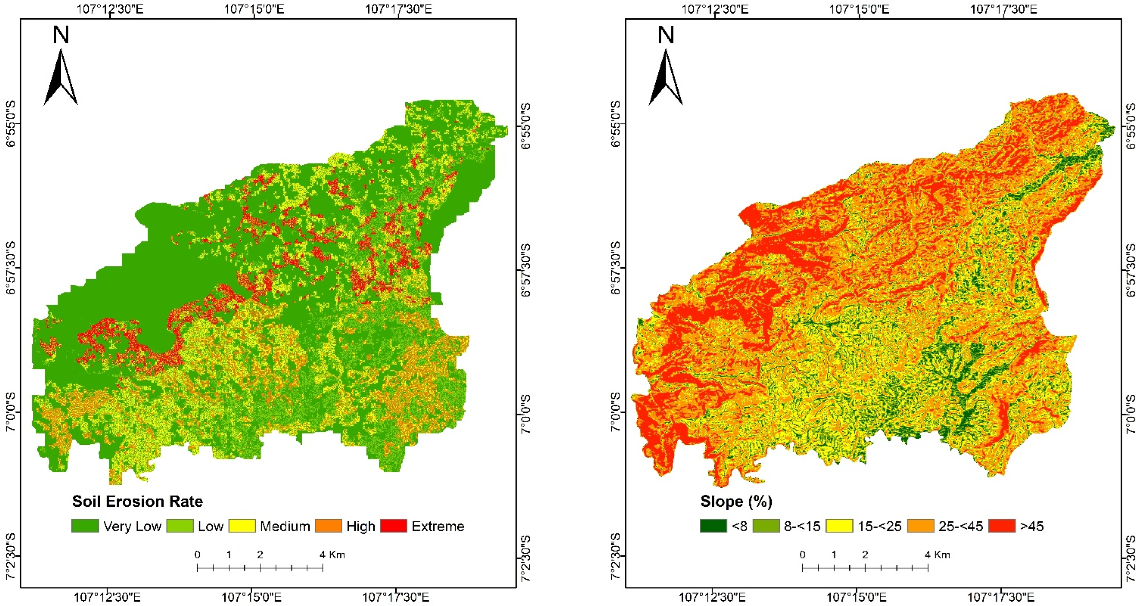
A slope analysis and the USLE soil erosion model were used to confirm the extreme landscape characteristics of Rongga Sub-district. The hilly and mountainous landscape of Rongga Sub-district was divided into five slope classes, expressed in percentages, where slope gradients of <8%, 8%–15%, 15%–25%, 25%–45%, and >45% are considered flat, gentle, moderate, steep, and extremely steep, respectively [29]. The slope distribution of Rongga Sub-district’s landscape is shown in Figure 2.
Rongga Sub-district is dominated by steep slopes (25%–25%), covering 4505.37 hectares of the area, followed by moderate slopes (15%–25%), covering 2701.14 hectares of the total area, and extremely steep slopes (>45%), covering 2442.73 of the total area. Meanwhile, the area which was considered a flat slope (0%–8%) covered 708.77 hectares of the total area, indicating this category as the slope category with the smallest area in the Rongga Sub-district landscape. These results also indicate that Rongga Sub-district’s landscape is dominated by steep to extremely steep slopes, with gradients over 25% covering most of the area, as shown in Table 3. Agricultural practice on steep slopes, however, is very susceptible to hydrogeological instability [42]. Furthermore, the lack of maintenance of the cultivated land, extreme rainfall erosivity, very weak soil erodibility, and intensive contouring and tillage practices in the area, may worsen the susceptibility to soil erosion [43].
An erosion risk assessment for the Rongga Sub-district landscape was performed by overlaying five USLE factors using the raster calculator QGIS spatial analyst. The process generated a soil erosion intensity map of the area. The map expresses the intensity of five classes of soil erosion in tons per hectare per year, i.e., very weak (<16), weak (16–60), moderate (60–180), strong (180–480), and extreme (>480). The soil erosion distribution map (Figure 2) shows that the average annual soil loss in the Rongga Sub-district landscape is 103.03 ton/ha/year, and the maximum value of soil erosion is approximately 3195.28 ton/ha/year, which occurred in the area which was not covered by vegetation or was considered as bare lands and extremely steep slopes.
Table 4 show the area of estimated soil erosion occurrence for every intensity class. The estimation of soil erosion area showed that approximately 6816.40 ha (about 60%) of the Rongga Sub-district landscape indicated very weak soil erosion and thus very low erosion risk. Meanwhile, 4592.11 ha (about 40%) of the total Rongga Sub-district area shows a high soil erosion risk. The second most extensive area comprised moderate-intensity soil loss and consequently moderate erosion risk, covering 1546.96 ha (about 14% of the total area). Weak-intensity or low soil erosion risk was in third place, covering 1504.93 ha (13%), followed by strong-intensity or high soil erosion risk, which covered 988.68 ha or about 9% of the total area. Lastly, the extremely high soil erosion risk area was the smallest at 551.53 ha or about 5% of the total area. These results show that the area of very low soil erosion risk is more extensive than that of higher classes of soil erosion risk. However, the area with steep slopes (25%–45%) had the highest average of estimated soil erosion potential at around 116.89 ton/ha/year. Moderate slopes (15%–25%) were next, with an estimated soil erosion average of 114.92 ton/ha/year. Ranking third was gentle slopes (8%–15%), with an estimated soil erosion average of 108.11 ton/ha/year. The estimated soil erosion average value of flat slopes (0%–8%) was not the lowest, being higher (99.68 ton/ha/year) than that of the extremely steep slope area (>45%), which was 81.54 ton/ha/year. These results imply that the soil erosion value shows an increasing trend as the slope gradient increases. However, this only occurred in the 0%–45% slope gradients as the extremely steep slope level (>45%) showed the lowest estimated soil erosion average, as shown in Table 5.
One study showed a positive correlation between the soil erosion average and slope gradient, i.e., the steeper the slope, the higher the estimated soil erosion average [44]. Runoff affected by tillage management may increase soil erosion on longer and steeper slopes [45]. Many other researchers also found that the soil erosion rate shows an exponentially increasing trend with an increasing slope gradient [46].

3.2. Structural Analysis at the Land Cover Type Level

3.2.1. Landscape Elements (Composition) and Dominance

Fragstat 4.2.1 was used to determine the landscape composition and dominance based on the class area (CA) and percentage of landscape (PLAND), and the analysis results are shown in Table 6.
Table 1 and Figure 3 show that the landscape in Rongga Sub-district consists of nine elements, namely agroforestry, secondary forests, open fields, rainfed rice fields, plantations, shrubs, irrigated rice fields, settlements, and rivers. Most of the elements were covered with different (natural as well as artificial) vegetation types. The values of CA and PLAND varied, with the highest value shown by the dry land forest patches with an area of 3498.165 ha, i.e., 29.8% of the entire landscape area. The open fields were next, covering an area of 2053.6875 ha, or 17.5% of the landscape, and the third was agroforestry at 13.05%, with an area of 1528.74 ha. A high CA value indicates that the landscape element is the dominant element. A matrix is the most extensive landscape element and has a dominant role in the overall landscape function [28,47]. This suggests that the secondary forest was the matrix in the landscape of Rongga Sub-district.
Forests are an important functional component of a landscape [48]. Secondary forests play a role in environmental protection, wildlife conservation, culture, and economic function. The existence and maintenance of forest ecosystems have a positive impact in terms of improving the quality of the environment and the quality of life of the community [49]. Forests play an important role in soil and water conservation, carbon sequestration and oxygen release, biodiversity conservation, recreation, nutrient accumulation, air filtration, and commodity production [50].
Landscapes dominated by forest matrix patches have high connectivity [51]. The composition of the landscape matrix of the surrounding forest fragments is vital for the survival of some animal species because it offers a structure that helps animals move between fragments and other foraging areas [52].

3.2.2. The Number of Constituent Elements

The elements in the landscape varied in number, as indicated by the number of patches (NP). The results of the analysis using Fragstat 4.2.1 are shown in Table 7.
The number of patches (NP) can be used to measure the spatial heterogeneity of an entire landscape. This is because the NP can measure the quantity of each element that makes up the landscape. The NP is a direct indicator of the level of fragmentation [53]. As shown in Table 7, agroforestry patches were the most numerous in the landscape of Rongga Sub-district with 546 patches, followed by open fields with 429 patches and plantations with 368 patches. This suggests that these three landscape elements experienced severe fragmentation, which resulted in declining connectivity within and between the present main landscape elements in the study area.
The quantification results showed that the NP of agroforestry was the highest, which is in accordance with this element having the highest CA value. The NP of plantations was the third-highest, but the class area of this type was quite low (fifth out of the nine landscape elements). This showed that plantations were more fragmented compared to other landscape types [54].
The lowest number of patches was obtained for rivers. This was due to the low extent of the river area covered in the study area. In this study, the 1:75,000 scale map created with the Landsat 8 TIRS/OLI satellite data in Rongga Sub-district was not able to show the river areas due to limited pixels and resolution. River patches appeared too narrow and small, so they were less visible on the raster data.

3.2.3. Element Shapes

Elements’ patch shapes are an important parameter for describing the landscape structure. The metrics used to quantify this parameter were the landscape shape index (LSI), total edge (TE), and edge density (ED). The results of the analysis using Fragstat 4.2.1 with the LSI, TE, and ED metrics are shown in Table 8.
Based on the LSI results, the landscape elements were arranged from highest to lowest as follows: agroforestry > open fields > secondary forest > shrubs > plantations > rainfed rice fields > irrigated rice fields > settlements > rivers.
Agroforestry had the highest LSI value of 39.97. The value of LSI = 1 occurs when the landscape consists of a square plot or when it is the most compact (almost square) of an appropriate type; the LSI value continues to increase without limit when the type of patch becomes less compact and irregular [55]. An LSI value close to 0 indicates that the landscape has a simple form with high aggregation [56]. Values further from 0 show that the landscape has a complex shape with scattered plots that are segregated. This means that the agroforestry patches had an irregular and complex shape. The lowest LSI value was obtained for a river patch, indicating that this patch was simpler and almost elongated in form and was the most compact among the nine elements that constitute the landscape of Rongga Sub-district.
The total edge (TE) is an absolute measure of the total edge length of a particular element type. Table 8 show that the highest TE value was obtained for the dry land forest element, with a total edge length of 738,075 m. The dry forest element was more elongated compared to the other elements, which is consistent with its high CA, PLAND, and LSI values. The lowest TE value in this study was obtained for the river element due to its small segment in the study area.
Based on the ED values, the elements making up the landscape of Rongga Sub-district, arranged from highest to lowest value, are as follows: secondary forest > open fields > agroforestry > shrubs > plantations > rainfed rice fields > settlements > irrigated rice fields > rivers. The highest ED value in the Rongga Sub-district landscape was that of the dry land forest element at 63.05 m/ha. This shows that the dry land forest had the most irregular edge among the elements in Rongga Sub-district.

3.2.4. Element Distributions

The interspersion and juxtaposition index (IJI) was used as a metric to determine the element distribution. The IJI measures the extent to which different patch types are in proximity to each other [57]. The results of the analysis using Fragstat 4.2.1 with the IJI metric are shown in Table 9.
As can be seen from Table 9, the highest IJI value was for irrigated rice fields with a percentage of 90.62%, followed by settlements (90.51%) and rainfed rice fields (89.35%). IJI = 100% occurs when all types of patches are equally close to other patches. This suggests that irrigated rice fields were in close proximity to the other eight patches. In this study, the IJI percentage of the rivers was quite low (38.31%) compared to the other eight elements. The adjacency of the rivers, vis-à-vis the other elements, was uneven. Based on the classification of the land cover map, the river segments were only located in particular parts of the study area, such as in Sukaresmi and Bojong Salam villages.

3.3. Structural Analysis at the Landscape Level

At the landscape level, analyses were carried out to identify the distribution of elements and heterogeneity. The metrics used were NP, the Shannon Evenness Index (SHEI), and the Shannon Diversity Index (SHDI), and the results are shown in Table 10.

3.3.1. Element Distribution

At the landscape level, the Shannon Evenness Index (SHEI) measures 0 and 1. The SHEI equals 0 if the landscape consists of only one patch (i.e., there is no diversity) and approaches 0 if the area distribution of the patch types becomes uneven (i.e., dominated by only one kind of patch).
Based on the results obtained, the SHEI value in the landscape of Rongga Sub-district was 0.87, which is close to 1; therefore, it can be said that the distribution of patches in this landscape was quite even. This means that none of the landscape elements dominated the study area.

3.3.2. Heterogeneity

Heterogeneity is a measure of how the parts of a landscape differ from one another [58]. A high degree indicates that the distribution of various landscape types is almost even, and there is relatively high heterogeneity. The Shannon Diversity Index (SHDI) represents the heterogeneity of the landscapes in a study area [59].
Based on the results obtained, the SHDI value in Rongga Sub-district was 1.92, showing that the heterogeneity of this landscape was quite high. Habitat fragmentation occurring in a landscape can increase the number of land plots and the value of the SHDI [60]. This condition was supported by the NP value of 2734.

3.4. Ecological Networks at the Landscape Level

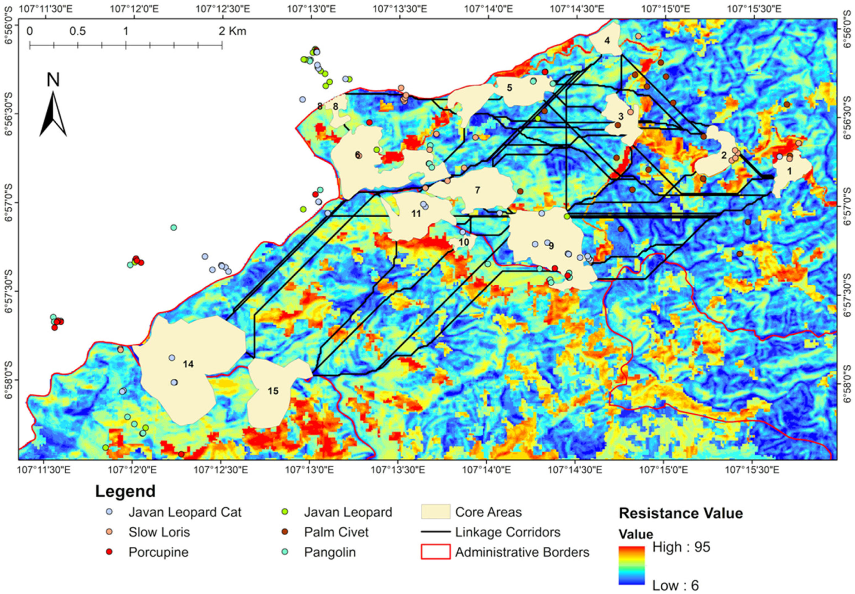
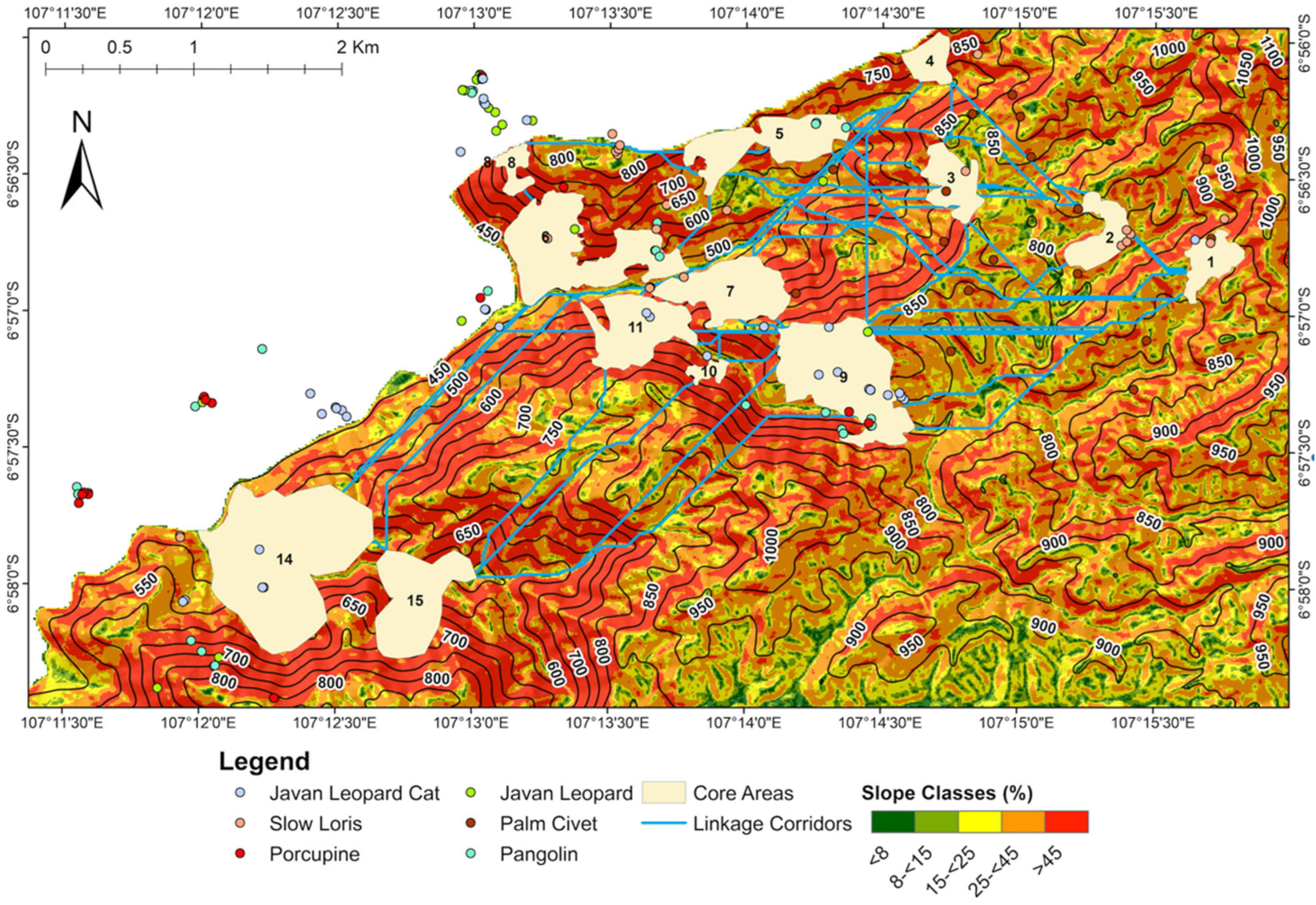
The implemented least-cost modeling resulted in a visual model of connectivity for multiple target species in the study area. The map of resistance surface distribution based on the experts’ judgment and combined pathways that will benefit the multiple target species is shown in Figure 4. The most favorable area networks were identified in the center of the species’ core areas. These networks link the eastern part and center of the region. We identified 11 ecological corridors connecting areas 1, 2, 3, 4, 5, 7, and 9 as the least-cost paths for the multiple target species’ movement in the study area. The lowest cost surface was measured from these particular core areas in terms of the resistance value. The most favorable vegetation cover with diverse tree species mostly exists in the remnant forest of the extreme landscape. These vegetation structures and compositions facilitate the movement of the targeted species, especially the arboreal species such as Nycticebus javanicus, and connect two or more larger areas of wildlife habitats. Although the center has relatively steep slopes, the area might have greater value due to its dominant forest cover. This resulted in the relatively low resistance value of the landscape matrices in the area.
The dry land forest located in the western part of the study area is more fragmented than in the eastern region. This is due to the fact that the western part consists of various land use patches of different sizes, such as shrubs, bare land, plantations, settlements, and rainfed rice fields. The ecological networks in the western part connect areas 6, 7, 9, 11, 14, and 15. The directions of the least-cost paths generally follow the most low-cost surface area. In some cases, the existence of wildlife corridors that pass through land cover with high resistance values is inevitable—for example, the networks connecting areas 1, 2, and 3 to area 9. In order to access area 9, every target species has to pass through an access road. This is in line with the findings of a previous study which found that certain species such as Nycticebus javanicus, Paradoxurus hermaphroditus, and Manis javanica were found passing the access road [61].
Rongga’s landscape, comprising agroforestry, secondary forests, and plantations, caused the contrast degree to be relatively low. This condition, together with the relatively good connectivity between the secondary forests, plantations, and agroforestry, is beneficial for the presence of wild animals needing heterogenous landscapes where the changes between one element and another are not drastic. It is clear that the extreme topography condition of Rongga Sub-district supports the landscape connectivity and, consequently, the presence of wild animals in this area (Figure 5). The relatively good connectivity might arise from the fact that the extreme landscape makes this area less accessible for humans and their activities.

3.5. Ecological Function

Agroforestry is a collective name for land-use systems and technologies where woody perennials (trees, shrubs, palms, bamboo, etc.) are deliberately used on the same land management units as agricultural crops and/or animal habitats, in some form of spatial arrangement or temporal sequence [62]. Agroforestry landscapes are defined as multiple land-use systems or a combination of forestry and agricultural landscapes that are managed to create a balance between agricultural intensification and forest sustainability [63,64]. Agroforestry land-use systems have the potential to increase agricultural land use while providing lasting benefits and reducing adverse environmental impacts at the local and global levels. This system promotes increased productivity and environmental stability by reducing emissions from deforestation and forest degradation [65].
As a system that combines trees and/or shrubs (perennial) with agronomic crops (annual or perennial), agroforestry can sequester carbon both above and below ground. Such agroforestry systems play an important role in increasing carbon stocks in the terrestrial biosphere [66].
One study revealed the existence of common palm civets in talun (mixed) gardens, which are the most suitable habitat type [16]. Palm civet cats eating palm fruit were found in agroforestry/talun gardens. This suggests that agroforestry provides food for the common palm civets. Another study revealed the existence of Javan slow lorises in Rongga Sub-district [17]. The Javan slow loris was mostly found around talun vegetation: sengon talun and mixed talun. This proves that this type of land use has the potential to become this animal’s habitat.
Secondary forests play an important role in conserving biodiversity, saving unique and endemic species that are adaptable to extreme conditions, and providing important ecosystem goods (e.g., livestock feed, firewood, medicine, and trade goods such as resin and sap) and services (e.g., formation and conservation of soil, conservation and quality improvement of water, setting of the water regime and microclimate, reducing the speed of the wind, control of wind erosion, and deceleration of the depletion of water) [67].
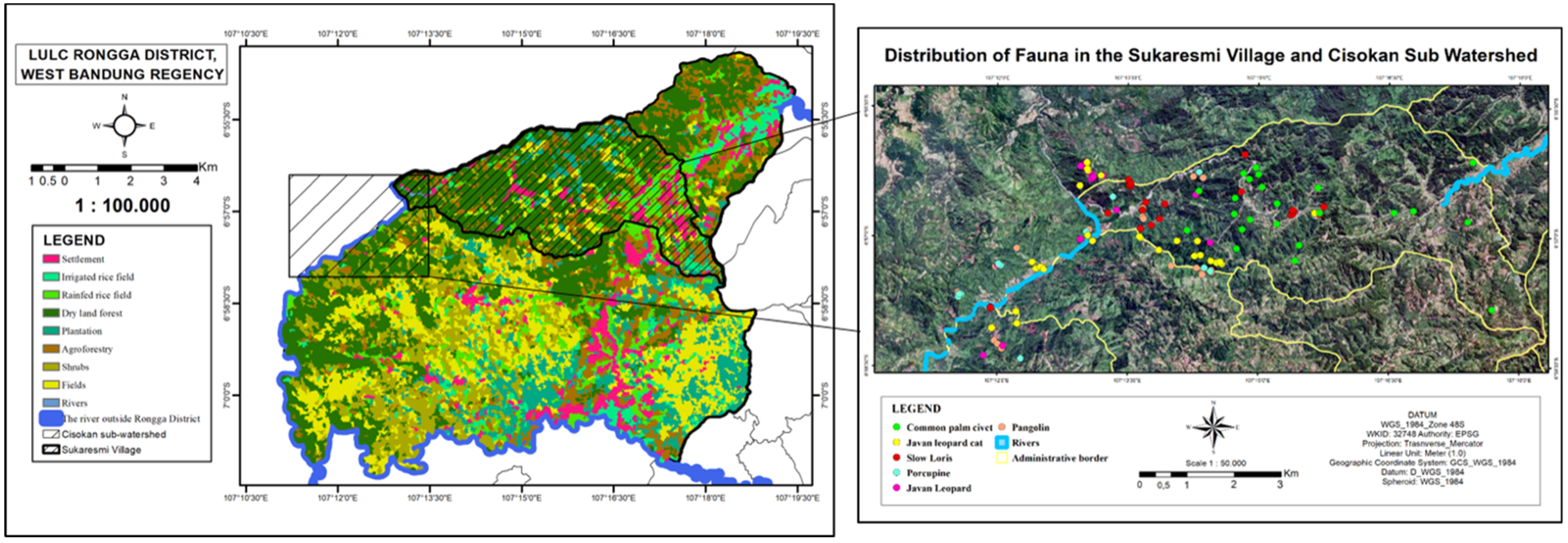
Figure 6 show some research that has revealed the presence of several animals in the dry land forests of Rongga Sub-district [16,17,18,19,20]. This research was specifically conducted in the future Cisokan sub-watershed area. One study successfully revealed the existence of the Javan leopard in both natural and production forests in Rongga Sub-district [18]. Furthermore, research revealed the existence of Javan leopards in natural forests [20]. The natural forests of Batu Nagok and Sarongge are far from human activities, and the main habitat of the Javan leopard is densely vegetated forests that are difficult to access, as well as areas with a steep topography (slope > 40%) and remote areas such as deep valleys or high hills that are difficult to reach.
One study revealed the existence of pangolins in Cisokan [19]. The points where pangolins were found in Rongga Sub-district were Batu Wulung, Curug (waterfall) Japarana, and Curug Walet. Additionally, subsequent research revealed the existence of slow lorises in Cisokan [17]. The point where slow lorises were found in Rongga Sub-district was in the Cilengkong area with secondary forest.
Dry land forests in Rongga Sub-district consist of both plantation and natural forests [40]. The plantation forests are pine (Pinus merkusii) production forests managed by Perhutani. Natural forests in Rongga Sub-district are mostly found on riverbanks along the Cisokan River, and the remaining natural forests are in Cigowek. Several types of plants that make up this natural forest, including Ficus sp., Piper aduncum, Artocarpus elasticus, Macaranga tanarius, and Spatodea campanulata, were found growing in river forests. Some of the typical forest tree types are Dysoxylum parasiticum, Dipterocarpus hasseltii, Ficus retusa, Artacarpus elasticus, Ficus variegata, and other Ficus sp.
Open field/moorland cover is used for dry land farming, especially for vegetables, chilies, and cassava [41]. The ecological function of farm fields is to mimic the structure of tropical forests, producing a lot of humus litter and burning biomass, which is very important as a nutrient for soil fertility. Farm fields also have a multilayered canopy that is structured stratigraphically and can withstand soil erosion [68]. At the landscape level, the cultivation system can keep the land well covered with vegetation, which helps reduce surface runoff and regulate water discharge [69].
A garden (plantation) is tree-growing land that is limited by ownership or other rights, has a canopy cover dominated by fruit or industrial trees, and has clear and regular boundaries [70]. Plantations in a landscape have important environmental benefits and play a role in sustainable production and improvement of soil quality, mitigation of water quality and carbon salinity, and biodiversity benefits [71]. In addition, plantations provide protection and a food source for local fauna and can even enhance the natural restoration of native forests [72,73]. Plantation patches can also improve landscape connectivity, acting as a species movement medium between remnants of the natural forest [74].
A settlement has a positive impact on the economic life of its residents but a negative effect on traditional village culture and the ecological landscape [75]. Human interaction with land through land uses such as building settlements and agriculture can affect the capacity of soil carbon storage, which is an important carbon reservoir that can be released as CO2 into the atmosphere [76].
The emergence of new settlements causes water absorption systems to be disrupted, drainage networks to not function properly, and household waste from the surface to be accumulated [77]. Based on the results of the landscape structure analysis, the area of settlement in Rongga Sub-district is 6.393%, showing that the landscape of Rongga Sub-district has not experienced much human intervention; thus, the ecological function of other patches was not disturbed. A study revealed the existence of common palm civets in the residential area of Sukaresmi Village, Rongga Sub-district [16], and other research revealed the existence of many Javan slow lorises in the vicinity of Rongga Sub-district settlements [17]. This proves that this type of land use has the potential to become a habitat.
Rice fields have various ecological functions; for instance, they can replace natural wetlands with artificial wetlands so that they act as habitats for freshwater animals, breeding areas, shelters, feeding places, other services for wildlife [78], and as oxygen producers, contributing to the conservation of land and water [79]. The rice field ecosystem also functions as a conservation area that supports the hydrological process, as a flood mitigation area that provides retention reservoirs, as an area that creates a microclimate and reduces pollutants, as a public recreation area, and as a disaster mitigation/evacuation area [80].
The rice field structure, which has a flat surface and is flanked by embankments, makes rice fields function as small dams to collect rainwater, thereby reducing the possibility of flooding. The ability to hold rainwater was initially intended to provide sufficient water for rice plants at the growth stage [81]. Thus, rice fields are analogous to wetlands as temporary places for rainwater [80]. Therefore, a rice fields’ ability to withstand rainwater and/or surface runoff is only useful when rain occurs to prevent flooding in lower areas or downstream [82].
Rice fields can also provide water purification. Rice fields can purify water if the incoming irrigation water contains high concentrations of nitrogen (N) and phosphorus (P). This purification occurs when the incoming nitrogen (N) concentration is 2–3 mg N/L or greater. The decrease in N concentration is caused by its reuse for crops and the denitrification of nitrate/nitrite-N in rice fields and irrigation/drainage systems [83].
Shrubs are used as ecological indicators because they form the majority of subcanopy structural layers in a forest. Shrub cover can indicate the habitat quality and a number of complex ecological processes that are interconnected [84]. Shrubs provide refuge and food for forest organisms. They also provide an input of essential organic materials to the ground, play a principal role in the nutrient cycle, contribute substantially to the diversity of compositions and structures, help protect watershed areas from erosion, and improve the aesthetics of a forest ecosystem [72]. For example, the coverage and distribution of shrubs affect the diversity and abundance of mycorrhizal fungi, which constitute important food for small mammals, which are important prey for avian and terrestrial predators [85].
Research has revealed the existence of common palm civets (Paradoxurus hermaphroditus) on the shrub cover in Sukaresmi Village in Rongga Sub-district [16]. This type of civet uses shrubs as a hiding place so as not to be seen by predators when looking for its food, especially at noon. Shrubs are the most suitable habitat type for civets due to the amount of food available for common palm civets in shrub-type habitats. Another study revealed that porcupines in the Cisokan sub-watershed were mostly found in shrubs [86].
Rivers have been widely used for settlements, infrastructure, and production. Rivers can provide drinking water, irrigation, fish as a food supply or for recreational fishing, and areas for flood protection [87]. Rivers play a role in regulating the flow of water and minerals originating from the surrounding land and influence the flow of materials and water [88]. Rivers carry soil and sediment from one place to another, which has a major impact on the landscape. The silt that settles in the river flood plains is channeled to several other elements, one of which is agricultural land, and agricultural land thus becomes fertile [89].
In addition, river flows play a role in the movement of geochemical and biological matter and energy in the environment and can become a habitat for river biota adapted to seasonally fluctuating flows. Rivers also provide spatial connectivity between habitats and allow for the spread of plants, animals, and fungi [90].

4. Conclusions

Based on our analysis, it can be concluded that the landscape of Rongga Sub-district consists of patch elements of agroforestry, open fields, settlements, shrubs, plantations, and rainfed as well as irrigated rice fields, with the dry land forest as a matrix and rivers as corridors. The prevalence of each element varies, with the highest score obtained for agroforestry, indicating a high degree of fragmentation. The patch shape was irregular and not compact, and the element distribution was fairly even: each patch was adjacent to other patch types, and the landscape heterogeneity was quite high. The vegetated landscape elements in the study area suggest that despite it being an extreme landscape, it might exhibit ecological functions, particularly in terms of wildlife protection and natural disaster prevention (e.g., against landslides and erosion).
Therefore, maintaining forest cover in the study area should be taken into account in natural resource management at the landscape level to safeguard the landscape integrity. Many elements of the Rongga Sub-district landscape play a role in environmental conservation, as indicated by the flow of energy and materials towards the patch level, as well as the mosaic level, and the presence of wildlife in some elements.
The use of Landsat images in this research means that the interpretation of the landscape was fragmented, which is a limitation of this study. The use of high-resolution orthophotos in future studies can help to gain a different interpretation of the cultural and complex landscapes.

Author Contributions

Conceptualization, S.W.; methodology, S.W., A.D.M. and M.A R.; software, A.D.M. and M.A.R.; validation, S.W., A.D.M. and M.A.R., P.P.; formal analysis, S.W., A.D.M. and M.A.R.; investigation, S.W., A.D.M., M.A.R.; resources, S.W., A.D.M. and M.A.R.; data curation, S.W., A.D.M. and M.A.R.; writing—original draft preparation, S.W; writing—review and editing, S.W., A.D.M. and P.P.; visualization, S.W., A.D.M. and M.A.R.; supervision, P.P.; project administration, S.W.; funding acquisition, P.P. All authors have read and agreed to the published version of the manuscript.

Funding

This research was funded by Ministry of Education and Culture through Universitas Padjadjaran.

Institutional Review Board Statement

Not applicable.

Informed Consent Statement

Not applicable.

Data Availability Statement

This study does not report any data.

Acknowledgments

The authors would like to thank the Indonesian Ministry of Education and Culture for supporting this research through Penelitian Dasar, Penelitian Terapan Unggulan Perguruan Tinggi, and Universitas Padjadjaran, Sumedang, Indonesia, for providing research funding through the Universitas Padjadjaran Academic Leadership Grant scheme.

Conflicts of Interest

The authors declare no conflict of interest.

References

  1. Turner, M.G.; Gardner, R.H. Landscape Ecology in Theory and Practice; Springer: New York, NY, USA, 2015; Volume 401. [Google Scholar]
  2. Wu, J.G. Landscape Ecology. In Encyclopedia of Theoretical Ecology; Hastings, A., Gross, L., Eds.; University of California Press: Berkeley, CA, USA, 2012; pp. 392–396. [Google Scholar]
  3. Council of Europe. European Landscape Convention, Florence 20. 10; European Treaty Series: Cardiff City, UK, 2000; No. 176; p. 7. [Google Scholar]
  4. Atik, M.; Işikli, R.C.; Ortaçeşme, V.; Yildirim, E. Definition of landscape character areas and types in Side region, Antalya-Turkey with regard to land use planning. Land Use Policy 2015, 44, 90–100. [Google Scholar] [CrossRef]
  5. Ingegnoli, V. Landscape Ecology: A Widening Foundation; Springer: Singapore, 2002. [Google Scholar]
  6. Tlapáková, L.; Stejskalová, D.; Karasek, P.; Podhrázská, J. Landscape Metrics as a Tool for Evaluation Landscape Structure—Case Study Hustopeče. Eur. Countrys. 2013, 5, 52. [Google Scholar] [CrossRef] [Green Version]
  7. Mitchell, C.; Reich, P.; Tilman, D.; Groth, J.V. Effects of elevated CO2, nitrogen deposition, and decreased species diversity on foliar fungal plant disease. Glob. Chang. Biol. 2003, 9, 438–451. [Google Scholar] [CrossRef]
  8. Brodie, J.F.; Redford, K.H.; Doak, D.F. Ecological Function Analysis: Incorporating Species Roles into Conservation. Trends Ecol. Evol. 2018, 33, 840–850. [Google Scholar] [CrossRef]
  9. van den Berg, E.; Santos, F.A.M. Aspectos da variação ambiental em uma floresta de galeria em Itutinga, MG, Brasil. Ciência Florestal. 2003, 13, 83–98. [Google Scholar] [CrossRef] [Green Version]
  10. Budke, J.C.; Jarenkow, J.A.; De Oliveira-Filho, A.T. Intermediary disturbance increases tree diversity in riverine forest of southern Brazil. Biodivers. Conserv. 2010, 19, 2371–2387. [Google Scholar] [CrossRef]
  11. Neary, D.G.; Ice, G.G.; Jackson, C.R. Linkages between forest soils and water quality and quantity. For. Ecol. Manag. 2009, 258, 2269–2281. [Google Scholar] [CrossRef]
  12. Clark, D.B.; Clark, D.A.; Rich, P.M.; Weiss, S.; Oberbauer, S.F. Landscape-scale evaluation of understory light and canopy structures: Methods and application in a neotropical lowland rain forest. Can. J. For. Res. 1996, 26, 747–757. [Google Scholar] [CrossRef]
  13. Forman, R.T.T. Land Mosaics: The Ecology of Landscapes and Regions; Cambridge University Press: Cambridge, UK, 1995. [Google Scholar]
  14. Zhao, Q.; Wen, Z.; Chen, S.; Ding, S.; Zhang, M. Quantifying Land Use/Land Cover and Landscape Pattern Changes and Impacts on Ecosystem Services. Int. J. Environ. Res. Public Health 2019, 17, 126. [Google Scholar] [CrossRef] [PubMed] [Green Version]
  15. Verma, A. Necessity of Ecological Balance for Widespread Biodiversity. Indian J. Biol. 2020, 4, 158–160. [Google Scholar] [CrossRef]
  16. Parikesit; Withaningsih, S.; Prastiwi, W.D. Estimated Abundance and Distribution of Common Palm Civet (Paradoxurus hermaphroditus, Pallas 1777) in the Rural Landscape of Sukaresmi, West Bandung Regency. IOP Conf. Ser. Earth Environ. Sci. 2019, 306, 012003. [Google Scholar] [CrossRef]
  17. Withaningsih, S.; Parikesit; Ayundari, A.; Prameswari, G.; Megantara, E.N.; Husodo, T. Distribution and habitat of Javan slow loris (Nycticebus javanicus É. Geoffroy, 1812) in non-conservation area. AIP Conf. Proc. 2018, 2019, 060006. [Google Scholar]
  18. Shanida, S.S.; Partasasmita, R.; Husodo, T.; Parikesit, P.; Megantara, E.N. Short Communication: Javan Leopard Cat (Prionailurus bengalensis javanensis Desmarest, 1816) in the Cisokan non-conservation forest areas, Cianjur, West Java, Indonesia. Biodiversitas 2018, 19, 37–41. [Google Scholar] [CrossRef]
  19. Withaningsih, S.; Noorahya, F.; Megantara, E.N.; Parikesit, P.; Husodo, T. Nest existences and population of Pangolin (Manis javanica Desmarest, 1822) at the designated area of Cisokan Hydropower, West Java, Indonesia. Biodivers. J. Biol. Divers. 2018, 19, 153–162. [Google Scholar] [CrossRef]
  20. Shanida, S.S.; Partasasmita, R.; Husodo, T.; Parikesit, P.; Febrianto, P.; Dan Megantara, E.N. Short Communication: The existence of Javan Leopard (Panthera pardus melas Cuvier, 1809) in the non-conservation forest areas of Cisokan, Cianjur, West. Java, Indonesia. Bodiversitas 2018, 19, 42–46. [Google Scholar] [CrossRef]
  21. West Bandung Regency Government. Medium-Term Investment Program Plan. West Bandung Regency, 2017–2022. 2015. Available online: https://sippa.ciptakarya.pu.go.id/sippa_online/ws_file/dokumen/rpi2jm/DOCRPIJM_cc06df8a09_BAB%20IBab%201%20RPIJM%20Kab%20Bandung.pdf (accessed on 18 November 2021).
  22. West Bandung Regency Government. Medium-Term Investment Program Plan. West Bandung Regency, 2015–2019. 2008. Available online: https://sippa.ciptakarya.pu.go.id/sippa_online/ws_file/dokumen/rpi2jm/DOCRPIJM_3a3c8d3e3b_BAB%20IIBAB%202.pdf (accessed on 17 November 2021).
  23. BPS. Rongga Subdistrict in Figures 2021. BPS-Statistics of Bandung Barat Regency. 2021. Available online: https://bandungbaratkab.bps.go.id/publication/2021/09/24/205c99047ff726dd984d59d0/kecamatan-rongga-dalam-angka-2021.html (accessed on 19 November 2021).
  24. Disdukcapil. Geographic Information System (GIS) Kab.Bandung Barat Kecamatan Rongga and 8 Village. 2019. Available online: http://disdukcapil.bandungbaratkab.go.id/Home/gis/rongga (accessed on 15 August 2020).
  25. Merchant, J.W.; Narumalani, S. Integrating Remote Sensing and Geographic Information Systems. In The SAGE Handbook of Remote Sensing, 1st ed.; Warner, A.T., Nellis, M.D., Foody, G.M., Eds.; SAGE Publications Ltd.: London, UK, 2009; pp. 257–268. ISBN 978-1-4129-3616-3. [Google Scholar]
  26. Wischmeier, W.H.; Smith, D.D. Predicting Rainfall Erosion losses—A Guide to Conservation Planning; U.S. Department of Agriculture Science and Education Administration: Washington, DC, USA, 1978.
  27. Prasetyo, L.B. Pendekatan Ekologi Lanskap Untuk Konservasi Biodiversitas; Faculty of Forestry, IPB University: Bogor, Indonesia, 2017. [Google Scholar]
  28. Forman, R.; Gordon, M. Landscape Ecology; John Wiley and Son: New York, NY, USA, 1986. [Google Scholar]
  29. Ministry of Forestry of Republic Indonesia. Regulation of the Director General of Watershed Management and Social Forestry on Guidelines for Identification of Watershed Characteristics; Ministry of Forestry: Jakarta, Indonesia, 2013.
  30. Boehner, J.; Selige, T. Spatial Prediction of Soil Attributes Using Terrain Analysis and Climate Regionalisation. In SAGA—Analysis and Modelling Applications; Boehner, J., Ed.; Verlag Erich Goltze GmbH: Gottingen, Germany, 2006. [Google Scholar]
  31. El Jazouli, A.; Barakat, A.; Ghafiri, A.; El Moutaki, S.; Ettaqy, A.; Khellouk, R. Soil erosion modeled with USLE, GIS, and remote sensing: A case study of Ikkour watershed in Middle Atlas (Morocco). Geosci. Lett. 2017, 4, 25. [Google Scholar] [CrossRef] [Green Version]
  32. Yustika, R.D.; Somura, H.; Yuwono, S.B.; Arifin, B.; Ismono, H.; Masunaga, T. Assessment of soil erosion in social forest-dominated watersheds in Lampung, Indonesia. Environ. Monit. Assess. 2019, 191, 726. [Google Scholar] [CrossRef]
  33. McGarigal, K.; Cushman, S.A.; Ene, E. FRAGSTATS v4: Spatial Pattern Analysis Program for Categorical and Continuous Maps. Computer Software Program Produced by the Authors at the University of Massachusetts, Amherst. 2012. Available online: http://www.umass.edu/landeco/research/fragstats/fragstats.html (accessed on 19 January 2020).
  34. Gurrutxaga, M.; Lozano, P.J.; del Barrio, G. GIS-based approach for incorporating the connectivity of ecological networks into regional planning. J. Nat. Conserv. 2010, 18, 318–326. [Google Scholar] [CrossRef]
  35. Etherington, T.R. Least-Cost Modelling and Landscape Ecology: Concepts, Applications, and Opportunities. Curr. Landsc. Ecol. Rep. 2016, 1, 40–53. [Google Scholar] [CrossRef] [Green Version]
  36. Tang, Y.; Gao, C.; Wu, X. Urban Ecological Corridor Network Construction: An Integration of the Least Cost Path Model and the InVEST Model. ISPRS Int. J. Geo-Inf. 2020, 9, 33. [Google Scholar] [CrossRef] [Green Version]
  37. Liu, C.; Newell, G.; White, M.; Bennett, A.F. Identifying wildlife corridors for the restoration of regional habitat connectivity: A multispecies approach and comparison of resistance surfaces. PLoS ONE 2018, 13, e0206071. [Google Scholar] [CrossRef]
  38. Holt, C.; Watts, K.; Bellamy, C.C.; Nevin, O.; Ramsey, A. Defining Landscape Resistance Values in Least-Cost Connectivity Models for the Invasive Grey Squirrel: A Comparison of Approaches Using Expert-Opinion and Habitat Suitability Modelling. PLoS ONE 2014, 9, e112119. [Google Scholar] [CrossRef] [Green Version]
  39. Walker, R.; Craighead, L. Analysing Wildlife Movement Corridors in Montana Using GIS; ESRI User Conference: San Diego, CA, USA, 1997. [Google Scholar]
  40. Permana, S.; Iskandar, J.; Parikesit, P.; Husodo, T.; Megantara, E.N.; Partasasmita, R. Changes of ecological wisdom of Sundanese People on conservation of wild animals: A case study in Upper Cisokan Watershed, West Java, Indonesia. Biodivers. J. Biol. Divers. 2019, 20, 1284–1293. [Google Scholar] [CrossRef] [Green Version]
  41. Yusuf, S.M.; Murtilaksonoc, K.; Hidayatc, Y.; Suharnotod, Y. Analysis and Prediction of Land Cover Changes in the Upper Citarum Basin. J. Pengelolaan Sumberd. Alam Dan Lingkung. 2018, 8, 365–375. [Google Scholar]
  42. Tarolli, P.; Preti, F.; Romano, N. Terraced landscapes: From an old best practice to a potential hazard for soil degradation due to land abandonment. Anthropocene 2014, 6, 10–25. [Google Scholar] [CrossRef]
  43. Pijl, A.; Tosoni, M.; Roder, G.; Sofia, G.; Tarolli, P. Design of Terrace Drainage Networks Using UAV-Based High-Resolution Topographic Data. Water 2019, 11, 814. [Google Scholar] [CrossRef] [Green Version]
  44. Rudiarto, I.; Doppler, W. Impact of land use change in accelerating soil erosion in Indonesian upland area: A case of Dieng Plateau, Central Java—Indonesia. Int. J. AgriSci. 2013, 3, 558–576. [Google Scholar]
  45. Chaplot, V.A.M.; Le Bissonnais, Y. Runoff Features for Interrill Erosion at Different Rainfall Intensities, Slope Lengths, and Gradients in an Agricultural Loessial Hillslope. Soil Sci. Soc. Am. J. 2003, 67, 844–851. [Google Scholar] [CrossRef]
  46. Jordan, G.; van Rompaey, A.; Szilassi, P.; Csillag, G.; Mannaerts, C.; Woldai, T. Historical land use changes and their impact on sediment fluxes in the Balaton basin (Hungary). Agric. Ecosyst. Environ. 2005, 108, 119–133. [Google Scholar] [CrossRef]
  47. Wandi, Y.; Manuwoto, S.; Buchori, D.; Hidayat, P.; Budiprasetyo, L. Spatial Analysis of Agricultural Landscapes and Diversity of Hymenoptera in Cianjur. HAYATI J. Biosci. 2006, 13, 137–144. [Google Scholar]
  48. Bargali, S.S. Forest Ecosystem: Structure and Functioning. Curr. Trends For. Res. 2018, 2, 1–3. [Google Scholar] [CrossRef]
  49. Ministry of Forestry of Republic Indonesia. Strategic Plan. 2010–2014; Ministry of Forestry: Jakarta, Indonesia, 2010.
  50. Mäler, K.G.; Aniyar, S.; Jansson, A. Accounting for Ecosystem Services as a Way to Under Stand the Requirements for Sustainable Development. Proc. Natl. Acad. Sci. USA 2008, 105, 9501–9506. [Google Scholar] [CrossRef] [PubMed] [Green Version]
  51. Goodwin, B.J.; Fahrig, L. How does landscape structure influence landscape connectivity? Oikos 2002, 99, 552–570. [Google Scholar] [CrossRef] [Green Version]
  52. Pozo-Montuy, G.; Serio-Silva, J.C.; Bonilla-Sanchez, Y.M. The influence of the matrix on the survival of arboreal primates in fragmented landscapes. Primates 2011, 52, 139–147. [Google Scholar] [CrossRef]
  53. Martins, R.N.; Abrahão, S.A.; Ribeiro, D.P.; Colares, A.P.F.; Zanella, M.A. Spatio-Temporal Analysis of Landscape Patterns in the Catolé Watershed, Northern Minas Gerais. Rev. Árvore 2018, 42, 1–11. [Google Scholar] [CrossRef] [Green Version]
  54. Ji, J.; Wang, S.; Zhou, Y.; Liu, W.; Wang, L. Spatiotemporal Change and Landscape Pattern Variation of Eco-Environmental Quality in Jing-Jin-Ji Urban Agglomeration from 2001 to 2015. IEEE Access 2020, 8, 125534–125548. [Google Scholar] [CrossRef]
  55. McGarigal, K. Fragstats Help. 2015. Available online: https://www.umass.edu/landeco/research/fragstats/documents/fragstats.help.4.2.pdf (accessed on 19 January 2020).
  56. Fynn, I.E.; Campbell, M.J. Forest Fragmentation Analysis from Multiple Imaging Formats. J. Landsc. Ecol. 2019, 12, 1–15. [Google Scholar] [CrossRef] [Green Version]
  57. Saritha, S.; Kumar, G.S. Analysis of the smart growth of kochi city through landscape metrics. In Proceedings of the 2017 IEEE Region 10 Symposium (TENSYMP), Cochin, India, 14–16 July 2017; pp. 1–5. [Google Scholar] [CrossRef]
  58. Gunawan, H.; Prasetyo, L.B. Forest Fragmentation: The Teory Underlying Forest Spatial Planning towards Sustainable Development; Research and Development Center for Conservation and Rehabilitation: Bogor, Indonesia, 2013. [Google Scholar]
  59. Lv, J.; Ma, T.; Dong, Z.; Yao, Y.; Yuan, Z. Temporal and Spatial Analyses of the Landscape Pattern of Wuhan City Based on Remote Sensing Images. ISPRS Int. J. Geo-Inf. 2018, 7, 340. [Google Scholar] [CrossRef] [Green Version]
  60. Herzog, F.; Lausch, A. Supplementing land-use statistics with landscape metrics: Some methodological considerations. Environ. Monit. Assess. 2001, 72, 37–50. [Google Scholar] [CrossRef] [PubMed]
  61. PLN. Biodiversity Management Plan (BMP) Monitoring Species Upper Cisokan Pumped Storage. (UCPS), Bandung, Indonesia. 2017; unpublished work. [Google Scholar]
  62. Nair, P.R. An Introduction to Agroforestry; Kluwer Academic Publisher: Dordrecht, The Netherlands, 1993. [Google Scholar]
  63. Kaswanto, F.; Tataq, A.; Choliq, M.; Bagus, S. Revitalizing Rural Landscape Yards as Landscape Service Providers to Improve Community welfare. J. Lanskap Indones. 2016, 8, 50–60. [Google Scholar] [CrossRef] [Green Version]
  64. Owonubi, J.J.; Otegbeye, G.O. Disappearing forest: A review of the Challenges for Conservation of genetic resources and environmental management. J. For. Res. Manag. 2002, 1, 1–11. [Google Scholar]
  65. Sobola, O.O.; Amadi, D.C.; Jamala, G.Y. The Role of Agroforestry in Environmental Sustainability. J. Agric. Vet. 2015, 8, 20–25. [Google Scholar] [CrossRef]
  66. Jacob, D.E.; Ufot, I.N.; Sotande, A.O. Climate Change Adaptation and Mitigation through Agroforestry Principles in the Sahal Region of Nigeria. In Proceedings of the 35th Annual Conference of the Forestry Association of Nigeria, Sokoto, Nigeria, 11–16 February 2013; pp. 300–308. [Google Scholar]
  67. Forest Conservation Team. Guidelines on Sustainable Forest Management in Drylands of Sub-Saharan Africa. Arid Zone Forests and Forestry Working Paper; No. 1; FAO: Rome, Italy, 2010. [Google Scholar]
  68. Iskandar, J. Cultivation Ecology in Indonesia; Djambatan: Jakarta, Indonesia, 1989. [Google Scholar]
  69. Mulyoutami, E.; van Noordwijk, M.; Sakuntaladewi, N.; dan Agus, F. Changes in Cultivation Pattern: A Shifting Perception of Cultivators in Indonesia; World Agroforestry Centre—ICRAF, SEA Regional Office: Bogor, Indonesia, 2010; p. 101. [Google Scholar]
  70. Badan Standarisasi Nasional. Klasifikasi Penutup Lahan SNI No 7645:2014. Bagian 1: Skala Kecil dan Menengah. 2014. Available online: www.bsn.go.id (accessed on 18 April 2020).
  71. Australian Goverment. Plantations and Farm Forestry. 2019. Available online: https://www.agriculture.gov.au/forestry/australias-forests/plantation-farm-forestry (accessed on 17 November 2020).
  72. Tellería, J.L.; Galarza, A. Avifauna Invernante En Un Eucaliptal Del Norte De España. Ardeola 1991, 38, 239–247. [Google Scholar]
  73. Humphrey, J. Benefits to biodiversity from developing old-growth conditions in British upland spruce plantations: A review and recommendations. Forestry 2005, 78, 33–53. [Google Scholar] [CrossRef]
  74. Brockerhoff, E.G.; Jactel, H.; Parrotta, J.A.; Quine, C.P.; Sayer, J. Plantation forests and biodiversity: Oxymoron or opportunity? Biodivers. Conserv. 2008, 17, 925–951. [Google Scholar] [CrossRef]
  75. Wang, Z.; Wang, C.; Jiang, Z.; Hu, T.; Han, W.; Zhang, C.; Jin, J.; Wei, K.; Zhao, J.; Wang, X. Relationship between Rural Settlements’ Plant Communities and Environmental Factors in Hilly Area of Southeast China. Sustainability 2020, 12, 2771. [Google Scholar] [CrossRef] [Green Version]
  76. Liang, M. Interaction of Human Settlement, Vegetation Patterns and Soils in the Northern Minnesota Prairie-Forest Region from the Euro-American Settlement Era to Present. Ph.D. Thesis, University of Wisconsin-Madison, Madison, WI, USA, 2017. [Google Scholar]
  77. Mukhoriyah. Study of the Ecological-Economic Value of Rice Fields and Its Relation to Spatial Planning in Depok City. Master’s Thesis, Universitas Indonesia, Jakarta, Indonesia, 2012. [Google Scholar]
  78. Zong, Y.; Chen, Z.; Innes, J.B.; Chen, C.; Wang, Z.; Wang, H. Fire and flood management of coastal swamp enabled first rice paddy cultivation in east China. Nat. Cell Biol. 2007, 449, 459–462. [Google Scholar] [CrossRef]
  79. Santosa, I.; Gusti, N.; Adnyana, G.M.; dan Dinata, I.; Ketut, K. The Impact of Rice Field Land Function Change on Rice Food Security. In Prosiding Seminar Nasional Budidaya Pertanian|Urgensi dan Strategi Pengendalian Alih Fungsi Lahan Pertanian|Bengkulu 7 July 2011; Universitas Bengkulu: Bengkulu, Indonesia, 2011; ISBN 978-602-19247-0-9. [Google Scholar]
  80. Natuhara, Y. Ecosystem services by paddy fields as substitutes of natural wetlands in Japan. Ecol. Eng. 2013, 56, 97–106. [Google Scholar] [CrossRef]
  81. Yoshikawa, N.; Nagao, N.; Misawa, S. Evaluation of the flood mitigation effect of a Paddy Field Dam project. Agric. Water Manag. 2010, 97, 259–270. [Google Scholar] [CrossRef]
  82. Masumoto, T.; Yoshida, T.; Kubota, T. An index for evaluating the flood-prevention function of paddies. Paddy Water Environ. 2006, 4, 205–210. [Google Scholar] [CrossRef]
  83. Maruyama, T.; Hashimoto, I.; Murashima, K.; Takimoto, H. Evaluation of N and P mass balance in paddy rice culture along Kahokugata Lake, Japan, to assess potential lake pollution. Paddy Water Environ. 2008, 6, 355–362. [Google Scholar] [CrossRef]
  84. Muir, P.S.; Mattingly, R.L.; Tappeiner, J.C., II; Bailey, J.D.; Elliot, W.E.; Hagar, J.C.; Miller, J.C.; Peterson, E.B.; Starkey, E.E. Managing for Biodiversity in Young Douglasfir Forests of Western Oregon. Biological Science Report USGS/I3RD/BSR-2002-0006; US Geological Survey, Biological Resources Division: Corvallis, OR, USA, 2002. [Google Scholar]
  85. Carey, A.B.; Kershner, J.; Biswell, B.; Dominguez De Toledo, L. Ecological Scale and Forest Development, Squirrels, Dietary Fungi, And Vascular Plants in Managed and Unmanaged Forest. Wildl. Monogr. 1999, 63, 3–71. [Google Scholar]
  86. Mustikasari, I.A.; Withaningsih, S.; Megantara, E.N.; Husodo, T.; Parikesit, P. Population and distribution of Sunda porcupine (Hystrix javanica F. Cuvier, 1823) in designated area of Cisokan Hydropower, West Java, Indonesia. Biodivers. J. Biol. Divers. 2019, 20, 762–769. [Google Scholar] [CrossRef] [Green Version]
  87. Böck, K.; Polt, R.; Schülting, L. Ecosystem Services in River Landscapes. In Riverine Ecosystem Management; Schmutz, S., Sendzimir, J., Eds.; Springer: Cham, Switzerland, 2018; Volume 8, pp. 413–433. [Google Scholar] [CrossRef]
  88. Wuisang, C.E.V.; dan Dwight, M.R. Greenbelt Planning in Urban Riverbank Landscapes. In Prosiding Temu Ilmiah IPB; Institut Pertanian Bogor: Bogor, Indonesia, 2015; pp. 103–108. [Google Scholar]
  89. Wuisang, C. Biodiversity Conservation in Urban Areas: Landscape Evaluation of Green Corridors in Manado City. Media Matrasain 2015, 12, 47–60. [Google Scholar]
  90. Mims, M.C.; Olden, J. Life history theory predicts fish assemblage response to hydrologic regimes. Ecology 2012, 93, 35–45. [Google Scholar] [CrossRef]
Figure 1. Borders of Rongga Sub-district (Source [25]).
Forests 13 00115 g001
Figure 2. Soil erosion and slope distribution map in Rongga Sub-district.
Forests 13 00115 g002
Figure 3. Land use/land cover of Rongga Sub-district.
Forests 13 00115 g003
Figure 4. Map of resistance values and ecological network among core areas.
Forests 13 00115 g004
Figure 5. Species distribution and linkage corridors map related to slope gradient.
Forests 13 00115 g005
Figure 6. Land use and distribution of fauna in Rongga Sub-district.
Forests 13 00115 g006
Table 1. The slope resistance values.
Slope Gradient (%)Resistance
0–1310
13–2320
23–3130
31–4040
40–4950
49–5860
58–6870
68–8180
81–10090
Table 2. The resistance values for land uses.
Land UseResistance
Settlement100
Irrigated Rice Field50
Rainfed Rice Field50
Dry Land Forests1
Plantations5
Agroforestry5
Shrubs10
Open Fields40
River90
Access Road80
Table 3. Slope classes in the Rongga Sub-district landscape.
Slope Gradient (%)LevelArea (ha)
0–8Flat708.76
8–15Gentle1348.38
15–25Moderate2701.14
25–45Steep4505.36
>45Extremely steep2442.73
Table 4. Classification of soil loss rate in the Rongga Sub-district landscape.
Soil Loss (ton/ha/year)IntensityArea (ha)Area (%)
<16Very weak6816.4060%
16–60Weak1504.9313%
60–180Moderate1546.9614%
180–480Strong988.689%
>480Extreme551.545%
Table 5. Estimated soil erosion average at every level of slope gradient.
Slope Gradient (%)LevelSoil Erosion Average (ton/ha/year)
0–8Flat99.67
8–15Gentle108.11
15–25Moderate114.92
25–45Steep116.88
>45Extremely steep81.54
Table 6. Calculation results of CA and PLAND metrics at the class level.
No.Type/ElementCA (ha)PLAND (%)
1Agroforestry1527.8013.06
2Secondary Forest3498.1729.88
3Open Fields2053.6917.54
4Plantations1136.959.712
5Settlements742.106.34
6Irrigated Rice Fields509.874.35
7Rainfed Rice Fields902.527.71
8Shrubs1326.3211.33
9Rivers8.890.07
Abbreviations: CA, class area; PLAND, percentage of landscape.
Table 7. Number of patches (NP) of each landscape element in the study area.
No.Type/ElementNP
1Agroforestry562
2Secondary Forest298
3Open Field429
4Plantation368
5Settlement203
6Irrigated Rice Fields245
7Rainfed Rice Fields305
8Shrubs314
9Rivers10
Table 8. LSI, TE, and ED metrics of each landscape type in the study area.
No.Type/ElementLSITE (m)ED (m/ha)
1Agroforestry39.97613,32052.39
2Secondary Forest32.34738,07563.05
3Open Fields35.94643,74054.99
4Plantations29.91395,82033.81
5Settlements22.07237,33020.27
6Irrigated Rice Fields23.05199,77017.06
7Rainfed Rice Fields27.72328,96528.11
8Shrubs30.36435,21037.17
9Rivers5.147100.40
Abbreviations: LSI, landscape shape index; TE, total edge; ED, edge density.
Table 9. Calculation results of IJI metric at the class level.
No.TypeIJI (%)
1Agroforestry75.92
2Secondary Forest77.83
3Open Fields85.68
4Plantations83.55
5Settlements90.51
6Irrigated Rice Fields90.62
7Rainfed Rice Fields89.35
8Shrubs72.41
9Rivers38.31
Abbreviation: IJI, interspersion and juxtaposition Index.
Table 10. Calculation results of NP, SHEI, and SHDI metrics at the landscape level.
LandscapeNPSHEISHDI
Rongga Sub-district27340.871.92
Abbreviations: NP, number of patches; SHEI, Shannon Evenness Index; SHDI, Shannon Diversity Index.
Publisher’s Note: MDPI stays neutral with regard to jurisdictional claims in published maps and institutional affiliations.

