Article

Fuel-Specific Aggregation of Active Fire Detections for Rapid Mapping of Forest Fire Perimeters in Mexico

by
Carlos Ivan Briones-Herrera
1,†,
Daniel José Vega-Nieva
1,*,†,
Jaime Briseño-Reyes
1,
Norma Angélica Monjarás-Vega
1,
Pablito Marcelo López-Serrano
1,
José Javier Corral-Rivas
1,
Ernesto Alvarado
2,
Stéfano Arellano-Pérez
3,
Enrique J. Jardel Peláez
4,
Diego Rafael Pérez Salicrup
5 and
William Matthew Jolly
6
1
Facultad de Ciencias Forestales, Universidad Juárez del Estado de Durango, Río Papaloapan y Blvd, Durango S/N Col. Valle del Sur, Durango C.P. 34120, Mexico
2
School of Environmental and Forest Sciences, University of Washington, Seattle, WA 98195, USA
3
Departamento de Ingeniería Agroforestal, Universidad de Santiago de Compostela, Escuela Politécnica Superior de Ingeniería, Campus Universitario s/n, C.P. 27002 Lugo, Spain
4
Centro Universitario de la Costa Sur, Universidad de Guadalajara, Av. Independencia Nacional No. 151, Autlán de Navarro C.P. 48900, Mexico
5
Instituto de Investigaciones en Ecosistemas y Sustentabilidad, Universidad Autónoma de México, Antigua Carretera a Pátzcuaro No. 8701, Col. Ex Hacienda de San José de la Huerta, Morelia C.P. 58190, Mexico
6
USDA Forest Service, Missoula Fire Sciences Laboratory, Missoula, MT 59808, USA
*
Author to whom correspondence should be addressed.
Contributed equally to this study.
Submission received: 3 December 2021 / Revised: 29 December 2021 / Accepted: 9 January 2022 / Published: 15 January 2022
(This article belongs to the Section Forest Inventory, Modeling and Remote Sensing)

Abstract

:
Context and Background. Active fires have the potential to provide early estimates of fire perimeters, but there is a lack of information about the best active fire aggregation distances and how they can vary between fuel types, particularly in large areas of study under diverse climatic conditions. Objectives. The current study aimed at analyzing the effect of aggregation distances for mapping fire perimeters from active fires for contrasting fuel types and regions in Mexico. Materials and Methods. Detections of MODIS and VIIRS active fires from the period 2012–2018 were used to obtain perimeters of aggregated active fires (AGAF) at four aggregation distances (750, 1000, 1125, and 1500 m). AGAF perimeters were compared against MODIS MCD64A1 burned area for a total of 24 fuel types and regions covering all the forest area of Mexico. Results/findings. Optimum aggregation distances varied between fuel types and regions, with the longest aggregation distances observed for the most arid regions and fuel types dominated by shrubs and grasslands. Lowest aggregation distances were obtained in the regions and fuel types with the densest forest canopy and more humid climate. Purpose/Novelty. To our best knowledge, this study is the first to analyze the effect of fuel type on the optimum aggregation distance for mapping fire perimeters directly from aggregated active fires. The methodology presented here can be used operationally in Mexico and elsewhere, by accounting for fuel-specific aggregation distances, for improving rapid estimates of fire perimeters. These early fire perimeters could be potentially available in near-real time (at every satellite pass with a 12 h latency) in operational fire monitoring GIS systems to support rapid assessment of fire progression and fire suppression planning.

1. Introduction

An accurate monitoring of burned area dynamics is key to support fire prevention, fire suppression, and post-fire environmental impact evaluation, including carbon cycle dynamics and emissions quantification [1,2,3]. Nevertheless, large uncertainties still exist in burned area quantification [4,5,6], limiting our ability to timely inform fire management decision-making.
Current products of global burned area, based on reflectance changes, are generally available monthly [7], while active fire detections, based on thermal anomalies, are available at least daily [8,9]. Furthermore, some studies have noted a better capacity of active fires to detect the presence of fires of smaller size compared to equivalent-resolution burned area products [3,10,11]. As a consequence, some studies, mainly at coarse scales of analysis, have aimed at relating gridded counts of active fires with burned area to improve global estimates of total burned area [8,10,11]. Such studies have mostly aimed at characterizing global trends of burned area and fire emissions [3,12] as opposed to an individual fire perimeter delineation at finer spatial scales.
In contrast to these approaches attempting to empirically relate the number of active fires to burned area at global to regional scales [13,14,15], other studies have aimed to map individual fire perimeters directly from the aggregated active fire data, using techniques such as point buffering [16,17] or convex hull algorithms [18,19]. In addition, some studies have utilized several spatial interpolation methods to map daily fire progression from active fires [20,21,22]. Most of those previous analyses of aggregated active fire (AGAF) perimeters have focused on the reconstruction of specific fire perimeters, mainly at a local scale of analysis (e.g., [18,22]), and have generally covered a limited temporal domain (e.g., [16,17]). There is, nevertheless, a need for evaluating AGAF over long periods of study and large areas, both for prediction of individual fire and total burned area. This appears to be necessary in order to test their large-scale potential for early rapid mapping of fire perimeters [19,23].
Furthermore, most of the previous literature on fire perimeter delineation from active fires has utilized mainly coarser resolution sensors, generally with 1 km resolution, such as MODIS (e.g., [16,18,20,21]). In contrast, the use of the VIIRS active fire product, with an improved spatial resolution (375 m) and higher capacity for small fire detection, still remains less-explored in the literature for direct mapping of fire perimeters [17]. In particular, the optimum parametrization for fire perimeter aggregation is still an area of ongoing research both for MODIS and VIIRS active fires [19,22].
An important aspect to consider is the quantification of the potential influence of fuel types and their associated climatic ecoregions in estimating the aggregation distance of active fires. Although this question has been suggested in previous studies based on gridded counts of active fires at a coarse scale [8,10,24], it does not yet seem to have been addressed by using the AGAF technique applied to individual fire perimeters. In fact, to our knowledge, we are not aware of any previous studies evaluating the role of fuel types on the performance of active fire clusters in predicting burned area, both at the level of individual fires and total monthly burned area, using AGAF techniques.
The goal of the current study was to analyze the influence of variations in the best aggregation distance for predicting burned area from the aggregation of MODIS and VIIRS active fires, for the main fuel types and ecoregions in Mexico, from 2012 to 2018. Aggregated active fire perimeters at distances of 750, 1000, 1125, and 1500 m were compared against the reference MCD64A1 burned area product [7]. The comparison was performed for individual fire perimeters and also for the total sum of burned area, for every fuel type and region in the study period. The study builds upon the previous analysis of Briones-Herrera et al. [23], which tested the potential of aggregated active fires for mapping monthly burned area at a national level in Mexico, utilizing a single aggregation distance. However, that study did not analyze potential variations between fuel types or ecoregions. This analysis could enhance our knowledge of the effects of fuel types on active fire aggregation distances, potentially improving early fire progression monitoring from active fires aggregation. To our best knowledge, there is no previous study attempting to analyze the effect of potential variations of the optimum aggregation distance of active fires on the prediction of burned area between different fuel types and biogeographical regions.

2. Materials and Methods

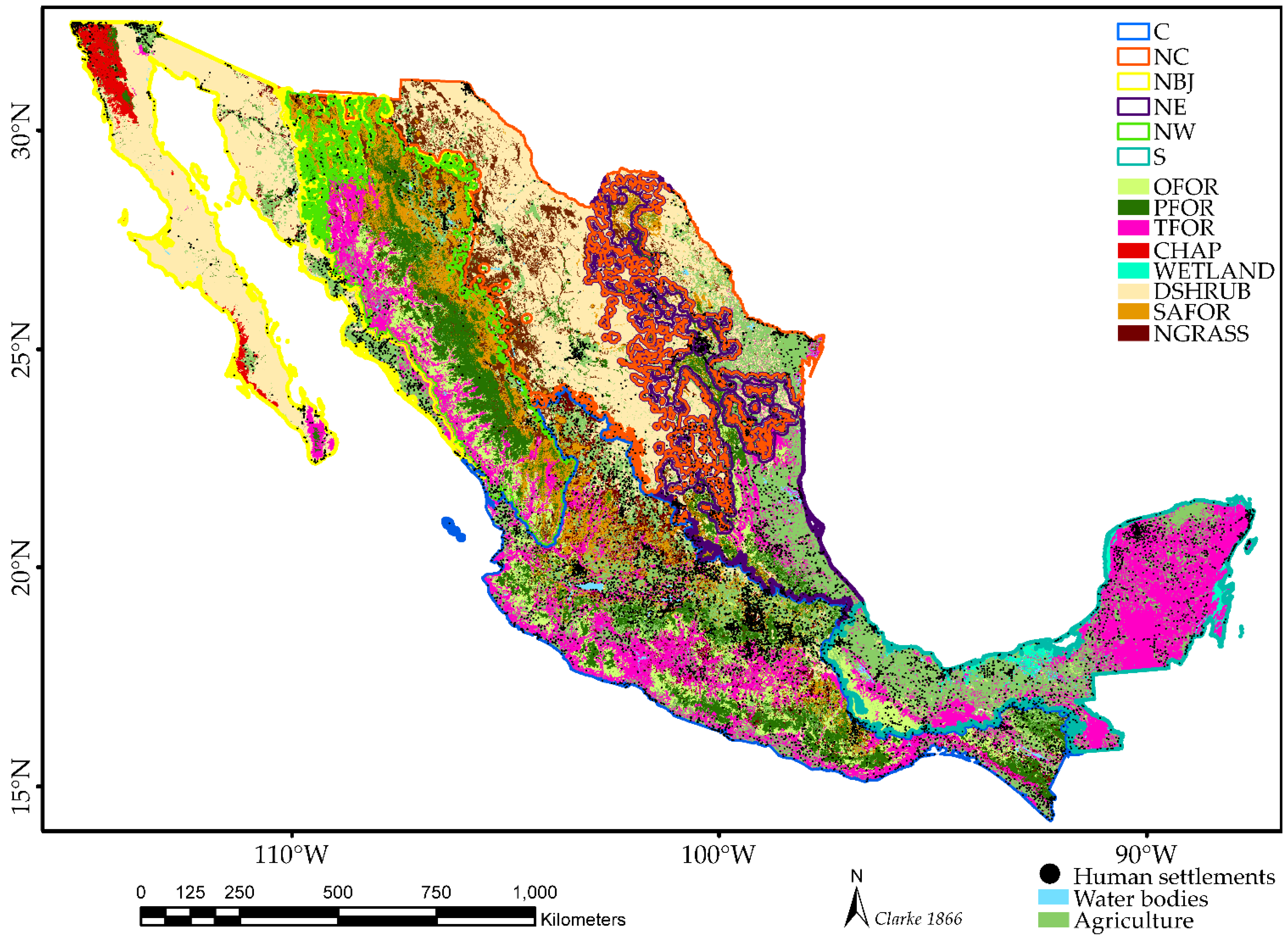
2.1. Study Area, Fuels and Regions Data

The area of study was the forest vegetation of the whole country of Mexico, excluding agricultural lands, water bodies, and human settlements, based on the latest land-use map (INEGI, 2014) [25] (Figure 1). Mexico is located in the northern hemisphere of the continent of America, it ranges between 32°43′06″–14°32′26″ N latitude and 86°42′36″–118°27′24″ W longitude. Within the area of study, a total of six regions were defined (Figure 1), following the regionalization of Briones-Herrera et al. [26], updated to the most recent land-use map [25]. The regions analyzed were based on the North American level 3 ecoregions map (EPA, https://www.epa.gov/eco-research/ecoregions-north-america, accessed on 28 December 2021), also considering the spatial and temporal patterns of fire occurrence observed in previous studies [27,28,29].
The analyzed regions (Figure 1) show contrasting climatic, human, and topographic characteristics, as summarized in Table 1. The highest mean precipitation occurs in the central and south (C and S) regions, while northern regions receive less precipitation (Table 1). C and S regions also concentrate a higher density of human population and of agriculture–forest interface (Table 1 and Figure 1). The vegetation of these two regions is dominated by temperate to tropical (C) and tropical forests (S), respectively, while shrubby and herbaceous arid to semiarid fuels are more abundant in northern regions, mainly in the drier NC and NBJ regions (Figure 1). Mean elevation ranges from 333.5 to 1640.8 m and average slope ranges from 2.4 to 7.5 % (Table 1).
Fuel types analyzed were based on the fuelbed map from Jardel-Peláez et al. [30] and on the latest land-use map (INEGI, 2014) [25] (Figure 1). Tropical forests include both seasonally dry and wet forests [30], the latter with scarcity of large fire observations. A total of 24 fuel and region types were considered for analysis, as shown in Figure 1.

2.2. Burned Area and Active Fires Data

The period analyzed comprised January 2012 to June 2018. Every month in the study period was utilized in the analysis. Collection C6 MODIS burned area (MCD64A1) products, with a pixel size of 500 m [7], were obtained from the FTP server of the University of Maryland. Active fire data from the Moderate Resolution Imaging Radiometer Spectrum (MODIS, C6) [9], and from the Visible Infrared Imaging Radiometer Suite (VIIRS, V1, 375 m) [31] were obtained from the Fire Information for Resource Management System (FIRMS, https://firms.modaps.eosdis.nasa.gov/download/create.php, accessed on 28 December 2021).

2.3. Predicting Perimeter from Aggregation of Active Fires by Fuel and Region

For the delineation of the active fire perimeters, a convex hull algorithm [23] was applied to monthly MODIS and VIIRS active fires, utilizing the “aggregate points” tool in ArcGIS (ESRI; 2011, Redlands, CA, USA) [32]. Monthly active fire perimeters were calculated at four analyzed aggregation distances of 750, 1000, 1125, and 1500 m. Following Briones-Herrera et al. [23], tested aggregation distances were based on the spatial resolution of the VIIRS and MODIS (375 and 1000 m, respectively) active fires. Monthly burned area for individual fire perimeters were obtained from monthly MCD64A1 data utilizing the “dissolve” and “aggregate polygon” tools in ArcGIS (ESRI; 2011, Redlands, CA, USA) [32].
AGAF perimeters and burned area MCD64A1 perimeters were combined with the fuel type and region map (Figure 1) and the corresponding area was calculated for every AGAF and burned area perimeter within each fuel and region. Spatially and temporally coinciding MCD64A1 burned area perimeters were compared with the corresponding AGAF perimeters in the same location, fuel type, and region, utilizing the “spatial join” tool in ArcGIS (ESRI; 2011, Redlands, CA, USA) [32] for every monthly dataset. If several AGAF perimeters fell within a MCD64A1 burned area perimeter by fuel type and ecoregion, their area was summed for analysis utilizing the burned area perimeter identifier in the combined dataset. Conversely, if several MCD64A1 burned area perimeters were associated spatially and temporally with a single AGAF perimeter by fuel type and region, their area was also summed for analysis, in order to avoid comparison of small burned area patches related to a larger event, that lay within the specified distance of analysis, against a corresponding AGAF perimeter.
For each fuel type and region, we used linear regression to compare monthly MCD64A1 burned area with the aggregated active fires perimeter at the four aggregation distances tested, utilizing Equation (1):
BA = a ∗ x
where
BA: MODIS C6 burned area (MCD64A1) (ha) by fuel type and region.
a: model coefficient.
x: aggregated perimeter of active fires (ha) by fuel type and region, respectively.
The models were analyzed at two levels for each fuel type and region:
(1)
Individual fire perimeter area.
(2)
Total monthly sum of burned area.
The best-performing models for predicting individual fire area for each fuel type and region were selected for evaluation at the total monthly sum level. Candidate equations were adjusted utilizing the “lm” package in R (R Core Team, 2017 Vienna, Austria) [33]. Model goodness-of-fit was evaluated by the coefficient of determination (R2), the root mean square error (RMSE), and the model bias [34], for every fuel and region dataset evaluated, at the two levels of analysis (individual fire and total monthly of burned area).
The dataset analyzed included a total of 5731 individual monthly fire perimeters. The analysis of the monthly sum of burned area considered a total of 79 monthly observations for every one of the 24 fuel types and regions analyzed.

3. Results

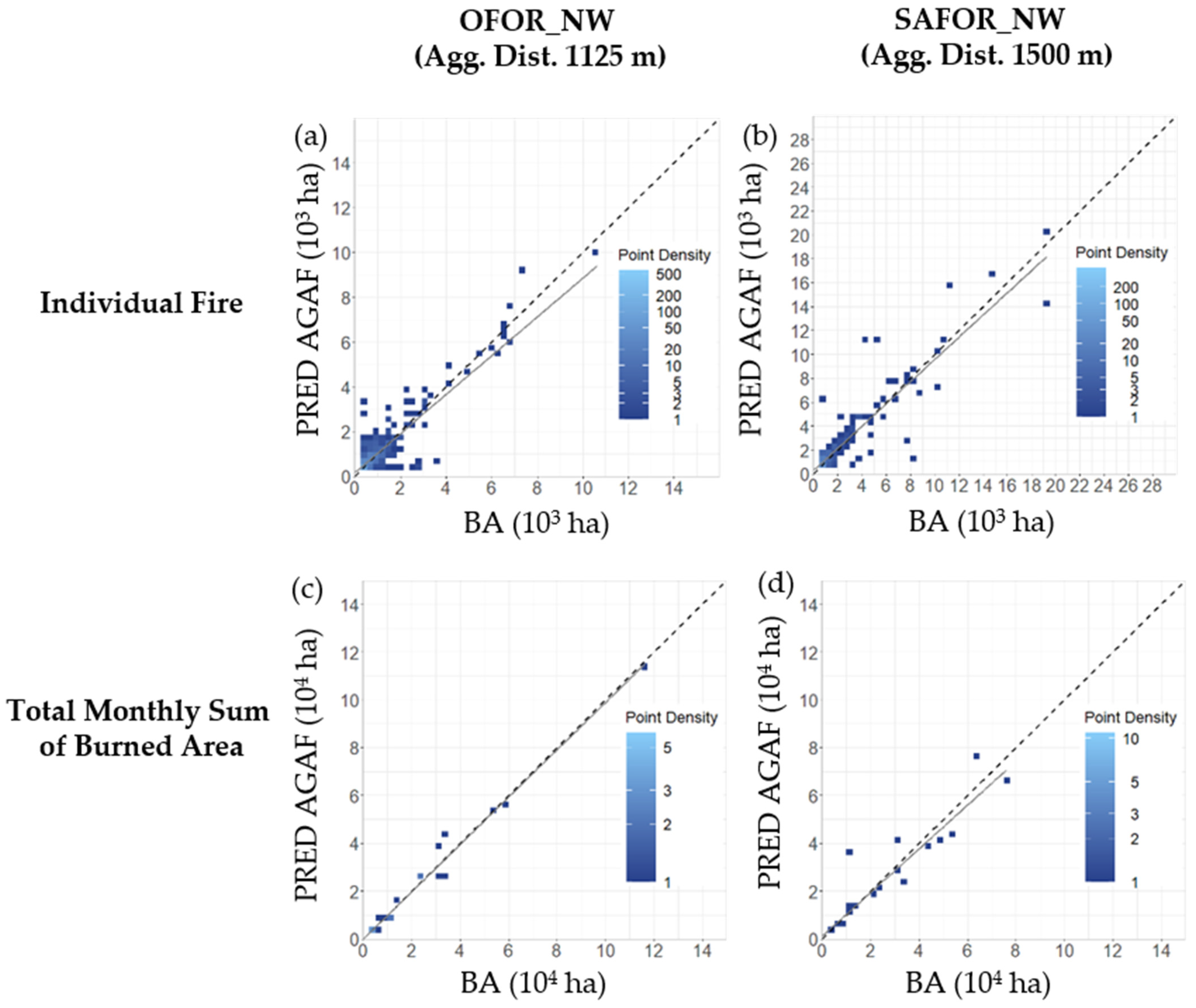
3.1. Best Fit Equations Relating Individual Fire Perimeter and Total Monthly Burned Area from Aggregated Active Fires by Fuel Type and Region

The largest average individual burned area sizes were observed for chaparral and semiarid forest of the NW region, with an average burned area of 1878 (+/−3098) and 1628 (+/−3056) ha, respectively. Lowest individual burned area values were observed for all tropical forests, with individual average fire sizes below 600 ha. Largest total monthly sum of burned area, of >400,000 ha, was observed for pine and oak forests of the C and NW regions, semiarid forests of the NW, and tropical forests of the C region, and lowest monthly burned area sums (<20,000 ha) were observed for fuel types in the more desertic NC and NBJ regions.
Best-performing active fire aggregation distances (750, 1000, 1125, 1500 m) varied between the different types of fuel and regions analyzed (Table 2). We also show the slope estimate and confidence interval of the parameters of each model (Equation (1)) and the values of the goodness-of-fit statistics for each fuel type and region (Table 2).
Burned area in fuel types dominated by fine fuels with low packing ratio, such as chaparral, desert shrubland, natural grasslands, and semiarid forests, had the best fit with the 1500 m aggregation distance (Table 2). Oak forests burned area had the best fit with 1125 m for C, NE, and NW regions, and 1500 m for the S region. Best fits for pine forests ranged from 1125 m for NW region to 1000 m for the NE and 750 m for the C region. For tropical forests, C, S, and NBJ regions had the best fit with a 1000 m aggregation distance, while regions of NW and NE had a best fit at 1500 m (Table 2).
For the individual fire perimeter level, the R2 was >0.7 for 11 fuelbeds and >0.5 for 18 of the 24 fuelbeds analyzed. Tropical forests of regions NW, S, and C had some of the lowest goodness-of-fits, with R2 in the range 0.5–0.3 (Table 2). For the total sum of monthly burned area, 11 of the analyzed fuelbeds showed a R2 > 0.9, and 19 of the 24 fuelbeds showed a R2 > 0.7. The fuelbeds with the lowest R2, in the range 0.6–0.5, for the total sum of monthly burned area were natural grasslands of NW and NBJ regions (Table 2). Examples of plots of aggregated active fire perimeters, against MODIS MCD64A1 burned area, for individual fire and total monthly sum of burned area, are shown in Figure 2.

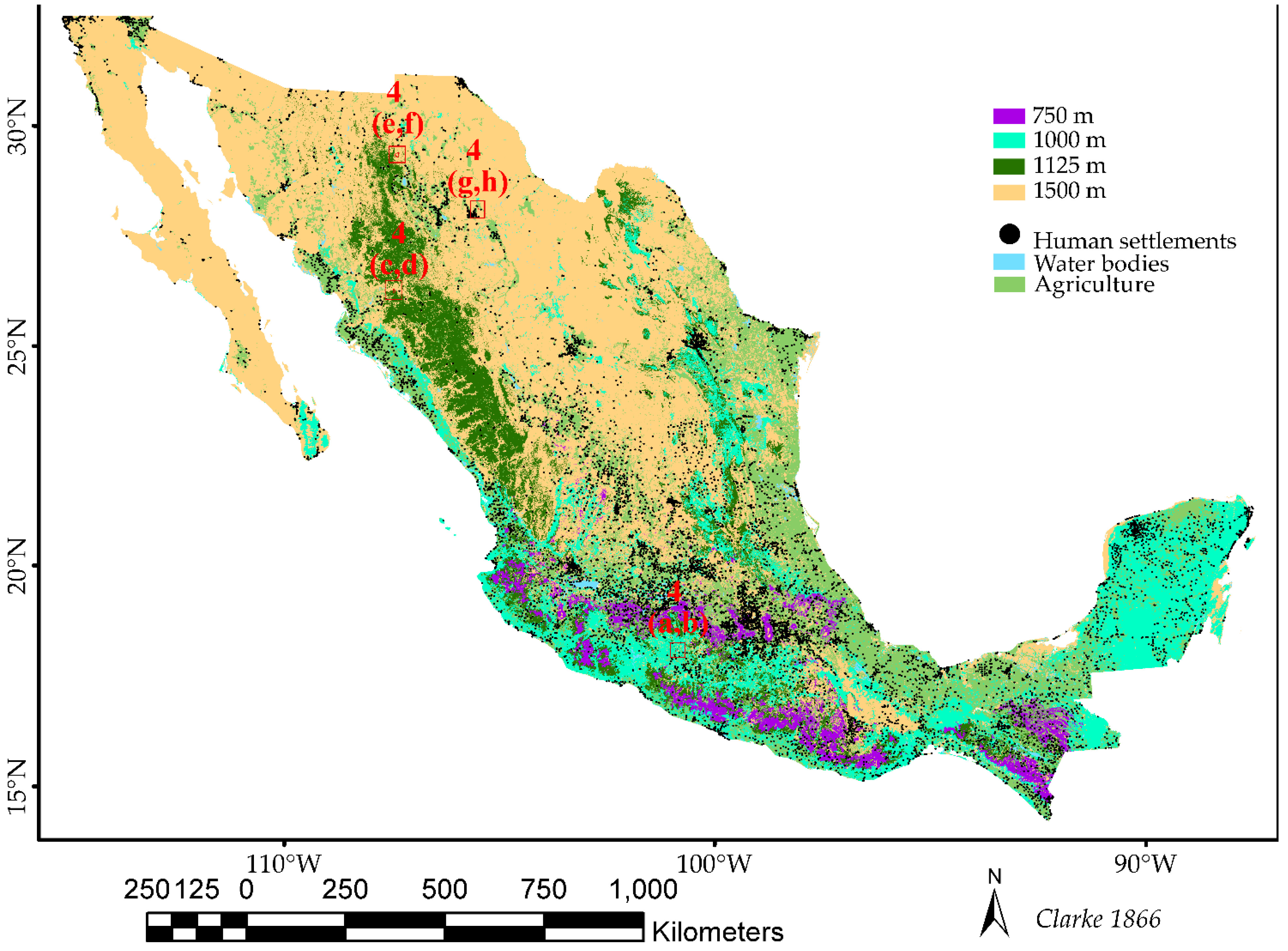
3.2. Spatial Distribution of the Best Aggregation Distances to Map Fire Perimeters from Active Fires by Fuel Type and Region

The spatial distribution of the best fit aggregation distances by fuel type and region is mapped in Figure 3. In general, drier areas with higher presence of finer and less-compacted fuels (chaparral, desert shrubland, natural grasslands, semiarid forests) showed the highest aggregation distances of 1500 m. Intermediate aggregation distances of 1125 m were observed for temperate forests (pine and oak forests in NW and NE, shown in dark green). The lowest aggregation distances of 750 and 1000 m appear to be mainly in areas dominated by tropical forest, or in temperate forests in the C and S regions, which receive higher precipitation (Table 1). The location of selected individual perimeter examples for local detail windows (Figure 4) are shown as red rectangles in Figure 3.

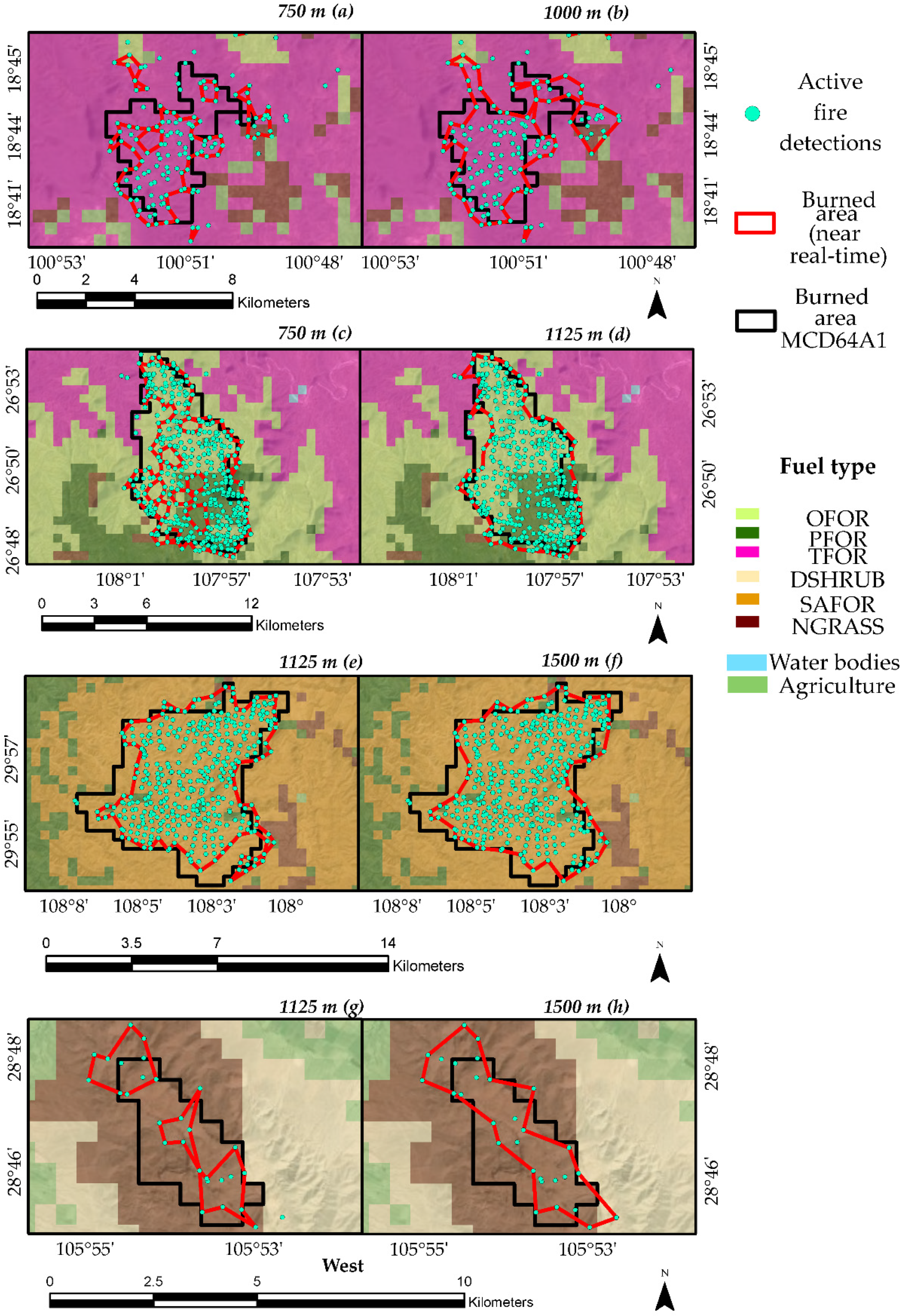
3.3. Examples of Aggregated Active Fire Perimeters with Varying Fuel-Specific Aggregation Distances against MODIS Burned Area

Selected examples comparing aggregated active fire perimeters with MODIS MCD64A1 burned area for various fuel types and regions with varying aggregation distances are shown in Figure 4. Background colors in Figure 4 represent fuel type. For the examples shown in tropical (Figure 4a,b) and temperate forests (Figure 4c,d), good agreements with MODIS burned area can be observed at 1000 (Figure 4b) and 1125 m (Figure 4d), respectively. In contrast, for the examples of the more arid fuel types semiarid forest (Figure 4e,f) and natural grassland (Figure 4g,h), burned area underestimation is observed at 1125 m (Figure 4e,g), while a better agreement with the burned area perimeter is observed at 1500 m (Figure 4f,h).

4. Discussion

The results from the current study revealed a clear variation of the active fire aggregation distances between regions. Such variations were documented with finer scales of analysis than previous studies that found regional variations in the relationships between active fire counts and burned area at coarser scales [10,11,13]. While our findings support these previous observations, the approach utilized (individual perimeter aggregation instead of gridded active fire counts), the temporal and spatial scale of analysis, and the spatial resolution of the satellites utilized here, differed from those previous studies. For example, the global scale analyses of Giglio et al. [8,10] and Randerson et al. [11] developed differentiated models to relate number of active fires to total sum of burned area for 14 continental regions at gridded scales of 0.25–0.5°. While this approach is valuable for developing global scale estimates of burned area and emissions [3,12], national level analyses can benefit from finer regionalization and spatial resolutions.
In our study, at a national scale, the analysis of active fire aggregation between regions suggests a climatic effect in fire spread potential between ecoregions (Figure 3). For example, the lowest active fire aggregation distances (750–1000 m) were more prevalent in areas with higher precipitation, such as temperate and tropical forests of the central and southern regions. This might be related to the known more-pronounced effect of moisture and fuel limitations on fire spread in these ecosystems [23,28]. In contrast, the highest aggregation distances (1500 m) were found in more arid ecosystems, such as the NC, dominated by lower tree canopies and larger shrubs and grass covers [30]. Intermediate aggregation distances (1000–1125 m) were observed for the temperate forests on the NW and NE regions. Interestingly, for some vegetation types, such as pine forests, lower aggregation distances were observed for the more humid NE region (1000 m), compared to relatively higher values (1125 m) observed for the pine forests of the NW region, which is characterized by higher fuel dryness conditions [28,29]. These results seem to support the potential of active fires to characterize differences in fire spread between regions [13]. Our study did not aim at the characterization of daily fire rate of spread [20,21,22] but focused on analyzing the fuel- and region-specific average aggregation distance to reproduce monthly perimeters. Nevertheless, as this average distance is also influenced by the distance between consecutive detections of active fires between satellite passes every 12 h, this parameter might be reflecting average variations in the potential of average fire spread between regions of different climatic and fuel conditions. Other weather and fuel-related fire behavior variables, such as variations in the duration of the smoldering phase of fuel combustion, mainly driven by duff load, bulk density, and moisture [35,36], might also be influencing the detected variations in active fire aggregation distances between fuels.
In addition to climate and fuels, other factors might also be affecting the observed variation in fire spread potential between regions. For example, the lower aggregation distances found in the C and S regions might be related to limitations in fuel continuity resulting from the high prevalence of agricultural interface and human population density [37]. This contrasts with higher aggregation distances observed in the northern regions that is potentially related to less human infrastructure and higher fuel connectivity [26,37]. Future studies in further characterizing fire regimes from satellite data might focus on analyzing the role of human variables [38,39,40,41], possibly including a formal evaluation of the role of fuel connectivity in fire spread and size [42,43].
A strong effect of fuel type was observed in our study, thereby corroborating that fuel availability influenced previously reported differences in the relationships between active fire counts and burned area, which had been observed at coarser scale, gridded counts, and levels of analysis [8,10,24]. Nevertheless, the approach used in such studies did not aim at determining aggregation distances to map individual fire perimeters, but to obtain regional estimates of total burned area, which were improved when considering regional and fuel-specific variations in the ratio of burned area to number of active fires.
For all of the regions analyzed, vegetation characterized by a higher fine fuel availability and lower bulk density, such as chaparral, desert shrubland, natural grassland, and semiarid forests, consistently showed the highest active fire aggregation distances, very possibly caused by the well-documented effect of those fine fuels on increasing rate of fire spread, compared to a lower rate of spread in forests with a more dense tree cover [44,45,46]. To our best knowledge, this is the first study to quantify such variations in the aggregation distance of MODIS and VIIRS perimeters, suggesting potential of accounting for a fuel-specific parametrization for improving individual fire perimeter mapping with AGAF techniques.
The results obtained can be useful to improve early operational estimates of fire perimeters from active fires. In particular, these initial results suggest that utilizing fuel- and region-specific active fire aggregation distances can help to better characterize fire perimeters, instead of considering constant values irrespective of fuel types and climatic regions, as currently used by the fire monitoring systems of Mexico [47,48] or elsewhere (e.g., [49]). The methodology to determine fuel- and region-specific aggregation distances presented here could be replicated in any other area of study, based on near-real-time available active fire data, combined with available maps of types of vegetation (e.g., [50,51]) or fuel types (e.g., [52]).
In the case of Mexico, these results can be implemented to improve the current aggregated active fire perimeters, which are available online at the national fire danger forecast system SPPIF (http://forestales.ujed.mx/incendios2/, accessed on 28 December 2021) [47,48]. The aggregated fire perimeters are published in SPPIF in near-real time at every satellite pass, a few minutes after the reception of MODIS and VIIRS active fire data by the antenna of CONABIO [53]. These perimeters are being used operationally every day by forest fire management agencies such as CONAFOR (National Forest Commission) to support fire progression monitoring and to guide operational fire management [54]. In particular, they are used to orient fire suppression decision-making such as defining the number, type, and location of fire suppression resources between states and even within individual fire events [47,48,54]. Such rapid active fire perimeters are currently being calculated at a single aggregation distance of 1125 m, based on the previous analysis at a national scale without considering fuel types or regions by Briones-Herrera et al. [23]. Based on the results from the current study, while this distance can be useful for characterizing fire perimeters in temperate to tropical fuels and regions, some underestimation could occur, compared to a better performance of the distance of 1500 m, for fires occurring in shrub and grass fuels, particularly in the more arid northern regions. Conversely, using the 1500 m distance in regions with high density of human populations and agricultural interface, such as C and S, could lead to the creation of artifacts by merging several adjacent burns in such areas where ignition density is higher [37], as illustrated by the examples at 1500 m shown in the previous study of Briones-Herrera et al. [23] (Figures 4 and 6 of the mentioned study).
AGAF perimeters can represent an improvement of the temporal availability (12 h intervals) compared to global burned area products [7] of 500 m, currently available at monthly intervals. In addition, AGAF perimeters can benefit from the capacity of thermal anomalies to better detect relatively smaller fires [10,11,23]. Nevertheless, a regression against medium resolution (10–30 m) perimeters for the smallest burns, characterized by 1 or 2 active fire detections, which do not result in an interpolated coarse-scale perimeter utilizing aggregation algorithms [23], might be required for a detailed evaluation of the contribution of smallest burns in total burned area [5]. Such very small burns are out of the scope of this coarse-scale early mapping technology, which can be later complemented with medium-scale imagery once it is available.
In this regard, ongoing research for calibrating Sentinel images (resolution = 10 and 20 m) to map fire perimeters and severity over a variety of fuel types and regions in Mexico [55] will likely allow comparisons of the procedure described in this paper to finer resolution perimeters. Furthermore, as suggested by Artés et al. [19] and Briones-Herrera et al. [23], early active fire perimeters, potentially obtained in near-real time, can serve to locate areas where higher spatial resolution imagery, of lower temporal resolution (5 days at least), can be downloaded once available. This can possibly be combined with semiautomated codes in platforms such as Google Earth Engine [56,57,58,59]. Such semiautomated codes can be initialized with the interpolated active fire perimeters [23], in order to support finer-scale fire perimeter and severity mapping [60,61,62,63,64]. Moreover, cross-country evaluations, potentially including data from countries where large datasets of medium resolution and even high spatial resolution thermal infrared aerial imagery are already available (e.g., [22,56,57,65]), could help to better refine the technique of active fire perimeter delineation. Such analysis would further contribute to a better understanding of the role of human, climatic, and fuel variables in fire spread potential.
In this sense, future studies could further analyze other drivers of fire spread beyond fuel type and ecoregions, including specific fuel characteristics such as tree height, canopy cover, or crown base height, potentially aided with LIDAR technologies (e.g., [66,67,68]). This could improve our landscape-scale knowledge of fire spread potential as affected by fuel characteristics, potentially enhancing fuel mapping initiatives (e.g., [69]) and fire behavior prediction efforts (e.g., [70,71]).

5. Conclusions

This study revealed the potential of accounting for the role of fuel type for defining the best aggregation distances when delineating large fire perimeters from aggregated active fires detected from moderate-resolution remote sensing. The highest active fire aggregation distances were observed in fuel types dominated by shrubs or grasslands, such as chaparral, desert shrubland, or semiarid forests. In contrast, the lowest distances were found for denser canopy temperate and tropical forests where fire spread is expected to be limited by a lower fine fuel availability and fuel moisture. Our results, developed at a finer spatial scale than previous coarse-scale studies with gridded active fire counts, support the observed general trend of increasing area burned per active fire with increasing presence of fine, dry, and loose fuel. In addition to fuel types, the distance of aggregation varied between regions of contrasting climatic and human presence conditions. In contrast to those previous coarse-scale gridded analyses, our approach quantified the relationship between burned area and active fire detections at a relatively finer spatial scale and did so by using point aggregation techniques at an individual fire perimeter and total sum of burned area levels over a relatively large temporal domain.
The analysis presented here could be replicated for any other region to derive fuel- and region-specific near-real time estimates of fire extent based on active fires and available vegetation or fuel-type maps and could improve the current decision-making in several processes of fire management. Future studies might also analyze further variability in active fire aggregation distances by additionally considering variations of fuel characteristics such as tree cover (e.g., [72]), tree height (e.g., [66]), or crown base height [67] within fuel types. Furthermore, the effects of seasonal or daily weather variations (e.g., [13,73,74]), including effects of wind on fire rate of spread (e.g., [75]), might be considered in future analysis of active fire aggregation at finer time scales. This could help to refine both fuel mapping and fire spread predictions based on remote sensing information [69,70,71].

Author Contributions

C.I.B.-H.: formal analysis, methodology; D.J.V.-N.: conceptualization, methodology, writing—original draft; J.B.-R.: programming; N.A.M.-V.: data curation; P.M.L.-S.: methodology; J.J.C.-R.: methodology; E.A.: writing—review and editing; S.A.-P.: writing—review and editing; E.J.J.P.: data curation, writing—review and editing; D.P.S.: writing—review and editing; W.M.J.: writing—review and editing. All authors have read and agreed to the published version of the manuscript.

Funding

Funding for this study was provided by CONAFOR/CONACYT Projects “CO2-2014-3-252620” and “CO-2018-2-A3-S-131553” for the development and enhancement of a Forest Fire Danger Prediction System for Mexico, funded by the Sectorial Fund for forest research, development and technological innovation “Fondo Sectorial para la investigación, el desarrollo y la innovación tecnológica forestal”.

Data Availability Statement

MODIS and VIIRS active fire data used in the study can be accessed from FIRMS: https://firms.modaps.eosdis.nasa.gov/active_fire/ (accessed on 28 December 2021). Aggregated active fire perimeters for the study period analyzed are publicly available through the Forest Fire Danger Prediction System of Mexico: http://forestales.ujed.mx/incendios2/ (accessed on 28 December 2021).

Acknowledgments

We would like to thank CONAFOR’s personnel for their support to the current study and their continuous feedback for the development of the Forest Fire Forecast Danger System of Mexico.

Conflicts of Interest

The authors declare no conflict of interest. The funders had no role in the design of the study; in the collection, analyses, or interpretation of data; in the writing of the manuscript, or in the decision to publish the results.

References

  1. Otón, G.; Pereira, J.M.C.; Silva, J.M.N.; Chuvieco, E. Analysis of Trends in the Fire CCI Global Long Term Burned Area Product (1982–2018). Fire 2021, 4, 74. [Google Scholar] [CrossRef]
  2. Chuvieco, E.; Mouillot, F.; Guido, R.; van der Werf, G.R.; San-Miguel-Ayanz, J.; Tanase, M.; Koutsias, N.; García, M.; Yebra, M.; Padilla, M.; et al. Historical background and current developments for mapping burned area from satellite Earth observation. Remote Sens. Environ. 2019, 225, 45–64. [Google Scholar] [CrossRef]
  3. Van der Werf, G.R.; Randerson, J.T.; Giglio, L.; van Leeuwen, T.T.; Chen, Y.; Rogers, B.M.; Mu, M.; van Marle, M.J.E.; Morton, D.C.; Collatz, G.J.; et al. Global fire emissions estimates during 1997–2016. Earth Syst. Sci. Data 2017, 9, 697–720. [Google Scholar] [CrossRef] [Green Version]
  4. Roy, D.; Boschetti, L.; Justice, C.O.; Ju, J. The Collection 5 MODIS Burned Area Product-Global evaluation by comparison with the MODIS active fire product. Remote Sens. Environ. 2008, 112, 3690–3707. [Google Scholar] [CrossRef]
  5. Roteta, E.; Bastarrika, A.; Padilla, M.; Storm, T.; Chuvieco, E. Development of a Sentinel-2 burned area algorithm: Generation of a small fire database for sub-Saharan Africa. Remote Sens. Environ. 2019, 222, 1–17. [Google Scholar] [CrossRef]
  6. Tariq, A.; Shu, H.; Li, Q.; Altan, O.; Khan, M.R.; Baqa, M.F.; Lu, L. Quantitative Analysis of Forest Fires in Southeastern Australia Using SAR Data. Remote Sens. 2021, 13, 2386. [Google Scholar] [CrossRef]
  7. Giglio, L.; Boschetti, L.; Roy, D.P.; Humber, M.L.; Justice, C.O. The Collection 6 MODIS burned area mapping algorithm and product. Remote Sens. Environ. 2018, 217, 72–85. [Google Scholar] [CrossRef]
  8. Giglio, L.; van der Werf, G.R.; Randerson, J.T.; Collatz, G.J.; Kasibhatla, P. Global estimation of burned area using MODIS active fire observations. Atmos. Chem. Phys. 2006, 6, 957–974. [Google Scholar] [CrossRef] [Green Version]
  9. Giglio, L.; Schroeder, W.; Justice, C.O. The collection 6 MODIS active fire detection algorithm and fire products. Remote Sens. Environ. 2016, 178, 31–41. [Google Scholar] [CrossRef] [Green Version]
  10. Giglio, L.; Randerson, J.T.; van der Werf, G.R.; Kasibhatla, P.S.; Collatz, G.J.; Morton, D.C.; DeFries, R.S. Assessing variability and long-term trends in burned area by merging multiple satellite fire products. Biogeosciences 2010, 7, 1171–1186. [Google Scholar] [CrossRef] [Green Version]
  11. Randerson, J.T.; Chen, Y.; van der Werf, G.R.; Rogers, B.M.; Morton, D.C. Global burned area and biomass burning emissions from small fires. J. Geophys. Res. 2012, 117, G04012. [Google Scholar] [CrossRef]
  12. Van der Werf, G.R.; Randerson, J.T.; Giglio, L.; Collatz, G.J.; Kasibhatla, P.S.; Arellano, A.F., Jr. Interannual variability of global biomass burning emissions from 1997 to 2004. Atmos. Chem. Phys. Discuss. Eur. Geosci. Union 2006, 6, 3175–3226. [Google Scholar] [CrossRef] [Green Version]
  13. Loboda, T.V.; Csiszar, I.A. Estimating burned area from AVHRR and MODIS: Validation results and sources of errors. In Proceedings of the 2nd Open All-Russia Conference: Current Aspects of Remote Sensing of Earth from Space, Moscow, Russia, 16–18 November 2004; Space Research Institute of the Russian Academy of Sciences, Publishing House GRANP: Moscow, Russia, 2004; pp. 415–421. [Google Scholar]
  14. Smith, R.; Adams, M.; Maier, S.; Craig, R.; Kristina, A.; Maling, I. Estimating the area of stubble burning from the number of active fires detected by satellite. Remote Sens. Environ. 2007, 109, 95–106. [Google Scholar] [CrossRef]
  15. Tansey, K.; Beston, J.; Hoscilo, A.; Page, S.E.; Paredes-Hernández, C.U. Relationship between MODIS fire hot spot count and burned area in a degraded tropical peat swamp forest in Central Kalimantan, Indonesia. J. Geophys. Res. 2008, 113, D23112. [Google Scholar] [CrossRef] [Green Version]
  16. Henderson, S.B.; Ichoku, C.; Burkholder, B.J.; Brauer, M.; Jackson, P.L. The validity and utility of MODIS data for simple estimation of area burned and aerosols emitted by wildfire events. Int. J. Wildland Fire 2010, 19, 844–852. [Google Scholar] [CrossRef]
  17. Oliva, P.; Schroeder, W. Assessment of VIIRS 375m active fire detection product for direct burned area mapping. Remote Sens. Environ. 2015, 160, 144–155. [Google Scholar] [CrossRef]
  18. Chiaraviglio, N.; Artés, T.; Bocca, R.; Lopez-Pérez, J.; Gentile, A.; San-Miguel-Ayanz, J.; Cortés, A.; Margalef, T. Automatic fire perimeter determination using MODIS hotspots information. In Proceedings of the IEEE 12th International Conference on e-Science (e-Science), Baltimore, MD, USA, 23–27 October 2016. [Google Scholar]
  19. Artés, T.; Boca, R.; Liberta, G.; San-Miguel-Ayanz, J. Non-supervised method for early forest fire detection and rapid mapping, Proc. SPIE 10444. In Proceedings of the Fifth International Conference on Remote Sensing and Geoinformation of the Environment (RSCy2017), 104440R, Paphos, Cyprus, 20–23 March 2017. [Google Scholar] [CrossRef] [Green Version]
  20. Parks, S.A. Mapping day-of-burning with coarse resolution satellite fire-detection data. Int. J. Wildland Fire 2014, 23, 215–223. [Google Scholar] [CrossRef]
  21. Veraverbeke, S.; Sedano, F.; Hook, S.J.; Randerson, J.T.; Jin, Y.; Rogers, B.M. Mapping the daily progression of large wildland fires using MODIS active fire data. Int. J. Wildland Fire 2014, 23, 655–667. [Google Scholar] [CrossRef] [Green Version]
  22. Scaduto, E.; Chen, B.; Jin, Y. Satellite-Based Fire Progression Mapping: A Comprehensive Assessment for Large Fires in Northern California. IEEE J. Sel. Top. Appl. Earth Obs. Remote Sens. 2020, 13, 5102–5114. [Google Scholar] [CrossRef]
  23. Briones-Herrera, C.I.; Vega-Nieva, D.J.; Monjarás-Vega, N.A.; Briseño-Reyes, J.; López-Serrano, P.M.; Corral-Rivas, J.J.; Alvarado-Celestino, E.; Arellano-Pérez, S.; Álvarez-González, J.G.; Ruiz-González, A.D.; et al. Near Real-Time Automated Early Mapping of the Perimeter of Large Forest Fires from the Aggregation of VIIRS and MODIS Active Fires in Mexico. Remote Sens. 2020, 12, 2061. [Google Scholar] [CrossRef]
  24. Hantson, S.; Padilla, M.; Corti, D.; Chuvieco, E. Strengths and weaknesses of MODIS hotspots to characterize global fire occurrence. Remote Sens. Environ. 2013, 131, 152–159. [Google Scholar] [CrossRef]
  25. INEGI (Instituto Nacional de Estadística y Geografía-México). Guía Para la Interpretación de Cartografía: Uso del Suelo y Vegetación. Escala 1,250,000; Serie VI. Instituto Nacional de Estadística y Geografía: Ciudad de México, México, 2014.
  26. Briones-Herrera, C.I.; Vega-Nieva, D.J.; Monjarás-Vega, N.A.; Flores-Medina, F.; Lopez-Serrano, P.M.; Corral-Rivas, J.J.; Carrillo-Parra, A.; Pulgarin-Gámiz, M.A.; Alvarado-Celestino, E.; González-Cabán, A.; et al. Modeling and mapping forest fire occurrence from aboveground carbon density in Mexico. Forests 2019, 10, 402. [Google Scholar] [CrossRef] [Green Version]
  27. Pompa-García, M.; Camarero, J.J.; Rodríguez-Trejo, D.A.; Vega-Nieva, D.J. Drought and spatiotemporal variability of forest fire across Mexico. Chin. Geogr. Sci. 2018, 28, 25–37. [Google Scholar] [CrossRef] [Green Version]
  28. Vega-Nieva, D.J.; Nava-Miranda, M.G.; Calleros-Flores, E.; López-Serrano, P.M.; Briseño-Reyes, J.; Corral-Rivas, J.J.; Cruz-López, M.I.; Cuahutle, M.; Ressl, R.; Alvarado-Celestino, E.; et al. Developing Models to Predict the Number of Fire Hotspots from an Accumulated Fuel Dryness Index by Vegetation Type and Region in Mexico. Forests 2018, 9, 190. [Google Scholar] [CrossRef] [Green Version]
  29. Vega-Nieva, D.J.; Nava-Miranda, M.G.; Calleros-Flores, E.; López-Serrano, P.M.; Briseño-Reyes, J.; Corral-Rivas, J.J.; Cruz-López, M.I.; Cuahutle, M.; Ressl, R.; Alvarado-Celestino, E.; et al. Temporal patterns of fire density by vegetation type and region in Mexico and its temporal relationships with a monthly satellite fuel greenness index. Fire Ecol. 2019, 15, 28. [Google Scholar] [CrossRef]
  30. Jardel-Peláez, E.J.; Alvarado, E.; Quintero-Gradilla, S.D.; Rodríguez-Gómez, J.M.; Pérez-Salicrup, D.; Michel-Fuentes, J.M.; Castillo-Navarro, M.F. Fuel Beds and Fire Potential in Mexican Terrestrial Ecosystems. Fire Ecol. 2021. under review. [Google Scholar]
  31. Schroeder, W.; Oliva, P.; Giglio, L.; Csiszar, I. The New VIIRS 375 m active fire detection data product: Algorithm description and initial assessment. Remote Sens. Environ. 2014, 143, 85–96. [Google Scholar] [CrossRef]
  32. ESRI. ArcGIS Desktop 10.1; Environmental Systems Research Institute: Redlands, CA, USA, 2011. [Google Scholar]
  33. R Core Team. R: A Language and Environment for Statistical Computing; R Foundation for Statistical Computing: Vienna, Austria, 2021; Available online: https://www.R-project.org/ (accessed on 28 December 2021)version 4.0.5.
  34. Ryan, T.P. Modern Regression Methods. In Wiley Series in Probability and Statistics; John Wiley and Sons: New York, NY, USA, 1997; 515p. [Google Scholar]
  35. Benscoter, B.; Thompson, D.; Waddington, J.M.; Wotton, M.; Flannigan, M.; de Groot, W.; Turetsky, M.R. Interactive effects of vegetation, soil moisture, and bulk density on depth of burning of thick organic soils. Int. J. Wildland Fire 2011, 20, 418–429. [Google Scholar] [CrossRef] [Green Version]
  36. Garlough, E.; Keyes, C. Influences of moisture content, mineral content and bulk density on smouldering combustion of ponderosa pine duff mounds. Int. J. Wildland Fire 2011, 20, 589–596. [Google Scholar] [CrossRef]
  37. Monjarás-Vega, N.A.; Briones-Herrera, C.I.; Vega-Nieva, D.J.; Calleros-Flores, E.; Corral-Rivas, J.J.; López- Serrano, P.M.; Pompa-García, M.; Rodríguez-Trejo, D.A.; Carrillo-Parra, A.; González-Cabán, A.; et al. Predicting forest fire kernel density at multiple scales with geographically weighted regression in Mexico. Sci. Total Environ. 2020, 718, 137313. [Google Scholar] [CrossRef] [PubMed]
  38. Archibald, S.; Roy, D.P.; van Wilgen, B.W.; Scholes, R.J. What limits fire? An examination of drivers of burnt area in Southern Africa. Glob. Change Biol. 2009, 15, 613–630. [Google Scholar] [CrossRef] [Green Version]
  39. Parisien, M.A.; Miller, C.; Parks, S.A.; DeLancey, E.R.; Robinne, F.-N.; Flannigan, M.D. The spatially varying influence of human on fire probability in North America. Environ. Res. Lett. 2016, 11, 075005. [Google Scholar] [CrossRef] [Green Version]
  40. Tariq, A.; Shu, H.; Siddiqui, S.; Munir, I.; Sharifi, A.; Li, Q.; Lu, L. Spatio-temporal analysis of forest fire events in the Margalla Hills, Islamabad, Pakistan using socio-economic and environmental variable data with machine learning methods. J. For. Res. 2021, 13, 12. [Google Scholar] [CrossRef]
  41. Tariq, A.; Shu, H.; Siddiqui, S.; Munir, I.; Nasri, A.; Waqas, H.; Baqa, M.F.; Lu, L. Forest fire Monitoring using spatial-statistical and Geo-spatial analysis of factors determining Forest fire in Margalla Hills, Islamabad, Pakistan. Geomat. Nat. Hazards Risk 2021, 12, 1212–1233. [Google Scholar] [CrossRef]
  42. Fernandes, P.M.; Monteiro-Henriques, T.; Guiomar, N.; Loureiro, C.; Barros, A.M. Bottom-up variables govern large-fire size in Portugal. Ecosystems 2016, 19, 1362–1375. [Google Scholar] [CrossRef]
  43. Kahiu, M.N.; Hanan, N.P. Fire in subSaharan Africa: The fuel, cure and connectivity hypothesis. Glob. Ecol. Biogeogr. 2018, 27, 946–957. [Google Scholar] [CrossRef] [Green Version]
  44. Scott, J.H.; Burgan, R.E. Standard Fire Behavior Fuel Models: A Comprehensive Set for Use with Rothermel’s Surface Fire Spread Model; General Technical Report RMRS-GTR-153; Department of Agriculture, Forest Service, Rocky Mountain Research Station: Fort Collins, CO, USA, 2005; 72p. [Google Scholar]
  45. Anderson, W.R.; Cruz, M.G.; Fernandes, P.M.; McCaw, W.L.; Vega, J.A.; Bradstock, R.A.; Fogarty, L.; Gould, J.; McCarthy, G.; Marsden-Smedley, J.B.; et al. A generic, empirical-based model for predicting rate of fire spread in shrublands. Int. J. Wildland Fire 2015, 24, 443–460. [Google Scholar] [CrossRef] [Green Version]
  46. Rodríguez-Trejo, D.A.; Pulido-Luna, J.A.; Martínez-Muñoz, P.; Martínez-Lara, P.J.; Monjarás-Vega, N.A. Comparative analysis of prescribed burns applied to tropical oak woodlands. Agrociencia 2018, 52, 783–801. [Google Scholar]
  47. Vega-Nieva, D.J.; Nava-Miranda, M.G.; Calleros-Flores, E.; López-Serrano, P.M.; Briseño-Reyes, J.; Corral-Rivas, J.J.; Cruz-López, M.I.; Cuahutle, M.; Ressl, R.; Alvarado-Celestino, E.; et al. The Forest Fire Danger Prediction System of Mexico. In Proceedings of the Remote Sensing Early Warning Systems: Virtual Wildfire Workshop, Online, 6–8 October 2020; Commission for Environmental Cooperation (CEC). Available online: http://forestales.ujed.mx/incendios2/php/publicaciones_documentos/Vega20_v2_The_Forest_Fire_Danger_Prediction_System_of_Mexico.pdf (accessed on 28 December 2021).
  48. Vega-Nieva, D.J.; Briseño-Reyes, J.; Briones-Herrera, C.I.; Monjarás, N.; Silva-Cardoza, A.; Nava, M.G.; Calleros, E.; Flores, F.; López-Serrano, P.M.; Corral-Rivas, J.J.; et al. User Manual of the Forest Fire Danger Forecast System of Mexico [Manual de Usuario del Sistema de Predicción de Peligro de Incendios Forestales de México]. Available online: http://forestales.ujed.mx/incendios2/php/publicaciones_documentos/1_1-%20MANUAL_DE_USUARIO_SPPIF_v15_DV290820.pdf (accessed on 28 December 2021). (In Spanish).
  49. San-Miguel-Ayanz, J.; Schulte, E.; Schmuck, G.; Camia, A.; Strobl, P.; Liberta, G.; Giovando, C.; Roberto Boca, R.; Sedano, F.; Pieter Kempeneers, P.; et al. Comprehensive Monitoring of Wildfires in Europe: The European Forest Fire Information System (EFFIS). In Approaches to Managing Disaster—Assessing Hazards, Emergencies and Disaster Impacts; European Commission, Joint Research Centre: Rome, Italy, 2012. [Google Scholar]
  50. ESA, European Space Agency. CCI Land Cover Product User Guide Version 2.4.; 449 ESA CCI LC project; ESA: Paris, France, 2014. [Google Scholar]
  51. Friedl, M.A.; Sulla-Menashe, D.; Tan, B.; Schneider, A.; Ramankutty, N.; Sibley, A.; Huang, X. MODIS Collection 5 global land cover: Algorithm refinements and characterization of new datasets. Remote Sens. Environ. 2010, 114, 168–182. [Google Scholar] [CrossRef]
  52. Pettinari, M.L.; Chuvieco, E. Generation of a global fuel data set using the Fuel Characteristic Classification System. Biogeosciences 2016, 13, 2061–2076. [Google Scholar] [CrossRef] [Green Version]
  53. Cruz-Lopez, M.I. Forest Fire Early Warning, Monitoring and Impact System in Mexico and Central America [Sistema de Alerta Temprana, Monitoreo e Impacto de los Incendios Forestales en México y Centroamérica]. In Proceedings of the 4th Wildland Fire International Conference, Sevilla, Spain, 14–17 May 2007; Available online: https://gfmc.online/doc/cd/REGIONALES/A_IBEROAMERICA/Cruz_MEJICO.pdf (accessed on 28 December 2021). (In Spanish).
  54. Robles-Gutiérrez, C.A. Application of the Forest Fire Danger Prediction System of Mexico in decision making. In Proceedings of the Remote Sensing Early Warning Systems: Virtual Wildfire Workshop, Online, 6–8 October 2020; Commission for Environmental Cooperation (CEC). Available online: http://forestales.ujed.mx/incendios2/php/publicaciones_documentos/Robles_20_Wildfire_Workshop_Panel_3__Application_SPPIF.pdf (accessed on 28 December 2021).
  55. Silva Cardoza, A.I. Evaluation and mapping of forest fires severity in the Western Sierra Madre, Mexico [Evaluación y mapeo de la severidad por incendios forestales en la Sierra Madre Occidental]; Sociedad Mexicana de Recursos Forestales. In Proceedings of the XIV Congreso Mexicano de Recursos Forestales, Durango, Mexico, 6–9 November 2019. (In Spanish). [Google Scholar]
  56. Parks, S.A.; Holsinger, L.M.; Voss, M.A.; Loehman, R.A.; Robinson, N.P. Mean Composite Fire Severity Metrics Computed with Google Earth Engine Offer Improved Accuracy and Expanded Mapping Potential. Remote Sens. 2018, 10, 879. [Google Scholar] [CrossRef] [Green Version]
  57. Whitman, E.; Parisien, M.A.; Holsinger, L.M.; Park, J.; Parks, S.A. A method for creating a burn severity atlas: An example from Alberta, Canada. Int. J. Wildland Fire 2020, 29, 995–1008. [Google Scholar] [CrossRef]
  58. Roteta, E.; Bastarrika, A.; Ibisate, A.; Chuvieco, E. A Preliminary Global Automatic Burned-Area Algorithm at Medium Resolution in Google Earth Engine. Remote Sens. 2021, 13, 4298. [Google Scholar] [CrossRef]
  59. Tariq, A.; Shu, H.; Gagnon, A.S.; Li, Q.; Mumtaz, F.; Hysa, A.; Siddique, M.A.; Munir, I. Assessing Burned Areas in Wildfires and Prescribed Fires with Spectral Indices and SAR Images in the Margalla Hills of Pakistan. Forests 2021, 12, 1371. [Google Scholar] [CrossRef]
  60. Fernández-García, V.; Santamarta, M.; Fernández-Manso, A.; Quintano, C.; Marcos, E.; Calvo, L. Burn severity metrics in fire-prone pine ecosystems along a climatic gradient using Landsat imagery. Remote Sens. Environ. 2018, 206, 205–217. [Google Scholar] [CrossRef]
  61. Sobrino, J.A.; Llorens, R.; Fernández, C.; Fernández-Alonso, J.M.; Vega, J.A. Relationship between Soil Burn Severity in Forest Fires Measured in Situ and through Spectral Indices of Remote Detection. Forests 2019, 10, 457. [Google Scholar] [CrossRef] [Green Version]
  62. García-Llamas, P.; Suárez-Seoane, S.; Fernández-Guisuraga, J.M.; Fernández-García, V.; Fernández-Manso, A.; Quintano, C.; Taboada, A.; Marcos, E.; Calvo, L. Evaluation and comparison of Landsat 8, Sentinel-2 and Deimos-1 remote sensing indices for assessing burn severity in Mediterranean fire-prone ecosystems. Int. J. Appl. Earth Obs. 2019, 80, 137–144. [Google Scholar] [CrossRef]
  63. French, N.H.F.; Graham, J.; Whitman, E.; Bourgeau-Chavez, L.L. Quantifying surface severity of the 2014 and 2015 fires in the Great Slave Lake area of Canada. Int. J. Wildland Fire 2020, 29, 892–906. [Google Scholar] [CrossRef]
  64. Llorens, R.; Sobrino, J.A.; Fernández, C.; Fernández-Alonso, J.M.; Vega, J.A. A methodology to estimate forest fires burned areas and burn severity degrees using Sentinel-2 data. Application to the October 2017 fires in the Iberian Peninsula. Int. J. Appl. Earth Obs. Geoinf. 2021, 95, 102243. [Google Scholar] [CrossRef]
  65. Eidenshink, J.; Schwind, B.; Brewer, K.; Zhu, Z.L.; Quayle, B.; Howard, S. A project for monitoring trends in burn severity. Fire Ecol. 2007, 3, 3–21. [Google Scholar] [CrossRef]
  66. Potapov, P.; Li, X.; Hernandez-Serna, A.; Tyukavina, A.; Hansen, C.M.; Kommareddy, A.; Pickens, A.; Turubanova, S.; Tang, H.; Silva, C.E.; et al. Mapping global forest canopy height through integration of GEDI and Landsat data. Remote Sens. Environ. 2020, 253, 112165. [Google Scholar] [CrossRef]
  67. González-Ferreiro, E.; Arellano-Pérez, S.; Castedo-Dorado, F.; Hevia, A.; Vega, J.A.; Vega-Nieva, D.; Álvarez-González, J.G.; Ruiz-González, A.D. Modelling the vertical distribution of canopy fuel load using national forest inventory and low-density airbone laser scanning data. PLoS ONE 2017, 12, e0176114. [Google Scholar] [CrossRef]
  68. Alonso-Rego, C.; Arellano-Pérez, S.; Guerra-Hernández, J.; Molina-Valero, J.A.; Martínez-Calvo, A.; Pérez-Cruzado, C.; Castedo-Dorado, F.; González-Ferreiro, E.; Álvarez-González, J.G.; Ruiz-González, A.D. Estimating Stand and Fire-Related Surface and Canopy Fuel Variables in Pine Stands Using Low-Density Airborne and Single-Scan Terrestrial Laser Scanning Data. Remote Sens. 2021, 13, 5170. [Google Scholar] [CrossRef]
  69. Peterson, B.; Nelson, K.J.; Seielstad, C.; Stoker, J.; Jolly, W.M.; Parsons, R. Automated integration of lidar into the LANDFIRE product suite. Remote Sens. Lett. 2015, 6, 247–256. [Google Scholar] [CrossRef]
  70. Cardil, A.; Monedero, S.; Ramírez, J.; Silva, C.A. Assessing and reinitializing wildland fire simulations through satellite active fire data. J. Environ. Manag. 2019, 231, 996–1003. [Google Scholar] [CrossRef]
  71. Botequim, B.; Fernandes, P.M.; Borges, J.G.; González-Ferreiro, E.; Guerra-Hernández, J. Improving silvicultural practices for Mediterranean forests through fire behaviour modelling using LiDAR-derived canopy fuel characteristics. Int. J. Wildland Fire 2019, 28, 823–839. [Google Scholar] [CrossRef]
  72. Sexton, J.O.; Song, X.-P.; Feng, M.; Noojipady, P.; Anand, A.; Huang, C.; Kim, D.-H.; Collins, K.M.; Channan, S.; Di Miceli, C.; et al. Global, 30-m resolution continuous fields of tree cover: Landsat-based rescaling of MODIS vegetation continuous fields with lidar-based estimates of error. Int. J. Digit. Earth 2013, 6, 427–448. [Google Scholar] [CrossRef] [Green Version]
  73. Freeborn, P.H.; Cochrane, M.A.; Jolly, W.M. Relationships Between Fire Danger and The Daily Number and Daily Growth of Active Incidents Burning in The Northern Rocky Mountains, USA. Int. J. Wildland Fire 2015, 24, 900–910. [Google Scholar] [CrossRef]
  74. Jolly, W.M.; Freeborn, P.H. Towards Improving Wildland Firefighter Situational Awareness Through Daily Fire Behaviour Risk Assessments in The US Northern Rockies and Northern Great Basin. Int. J. Wildland Fire 2017, 26, 574–586. [Google Scholar] [CrossRef]
  75. Billmire, M.; French, N.H.F.; Loboda, T.; Owen, R.C.; Tyner, M. Santa Ana winds and predictors of wildfire progression in southern California. Int. J. Wildland Fire 2014, 23, 1119–1129. [Google Scholar] [CrossRef]
Figure 1. Map of fuelbed types and regions of study, where C: central; NC: north central; NBJ: North Baja California; NE: northeast; NW: northwest; S: south region. OFOR: oak forests; PFOR: pine forests; TFOR: tropical forests; CHAP: chaparral forests; WETLAND: wetlands; DSHRUB: desert shrubland forest; SAFOR: semiarid forests; NGRASS: natural grasslands. Human settlements are shown in black, water bodies in blue, and agriculture in green, based on the Land-Use Map Series VI (INEGI, 2014) [25].
Forests 13 00124 g001
Figure 2. Predicted burned area from aggregated active fires (AGAF) against MODIS C6 MCD64A1 burned area (BA) for oak forests of the NW region (a,c) and semiarid forests of the NW region (b,d), at individual fire perimeter level (a,b) and total monthly sum of burned area level (c,d). OFOR: oak forests; SAFOR: semiarid forests (Figure 1); NW: northwest; Agg. Dist: aggregation distance; PRED AGAF: predicted burned area (using Equation (1)) from aggregated MODIS and VIIRS active fires at the specified aggregation distance; BA: MODIS C6 MCD64A1 burned area. The dotted black line shows the 1:1 line and the solid gray line shows the observed and predicted regression line. Point density values showing the number of observations by square plot division (in grey) are represented in a blue gradient.
Forests 13 00124 g002
Figure 3. Map of best active fire aggregation distances for fire perimeter mapping by fuel types and regions. Human settlements are represented in black, water bodies in navy blue, and agriculture in green, based on the most recent land-use map (INEGI, 2014) [25]. The location of detailed windows (Figure 4) is shown in red.
Forests 13 00124 g003
Figure 4. Examples of selected fire perimeters from April 2017 and May 2018 mapped using aggregated MODIS and VIIRS active fire data and MCD64A1 burned area, for tropical forest of the C region (a,b), oak forest of NW region (c,d), semiarid forest of the NW region (e,f), and grasslands of the NC region (g,h) at aggregation distances of 750 m (a,c), 1000 m (b), 1125 m (d,e), and 1500 m (f,h). MCD64A1 burned areas are represented in black, aggregated MODIS and VIIRS active fire perimeters are represented in red. Active fire detections are represented in bright blue. Background colors represent fuel types (Figure 1). Water bodies are shown in navy blue and agriculture in green, based on the most recent land-use map (INEGI, 2014) [25].
Forests 13 00124 g004
Table 1. Description of the regions of study.
NBJNWNCNECS
PD31.010.025.030.0159.049.0
(+/−68)(+/−40)(+/−76)(+/−87)(+/−441)(+/−74)
AGD0.52.60.410.313.824.4
(+/−0.8)(+/−3.2)(+/−1)(+/−6.7)(+/−12.0)(+/−16.2)
PREC280.1732.4371.4570.2978.71556.6
(+/−125.4)(+/−231)(+/−104.4)(+/− 268.2)(+/−321.2)(+/−442.1)
ELEV627.21640.81422.8986.81411.4333.5
(+/−389.4)(+/−716.1)(+/−581)(+/− 594.2)(+/−785.29)(+/−520.9)
Slope4.557.52.45.76.92.9
(+/−4.3)(+/−6.6)(+/−3)(+/− 6.1)(+/−6.0)(+/−3.9)
Values shown are average values; standard deviations are shown in brackets, PD: population density (residents/100 km2); AGD: agricultural interface density (km/100 km2); PREC: precipitation; ELEV: elevation; NBJ: North Baja California; NW: northwest; NC: north central; NE: northeast; C: central; S: south region.
Table 2. Coefficients and goodness-of-fit statistics of the best models when comparing burned area with aggregated fire perimeters produced with active fire data for each fuel and region.
Individual FireTotal Monthly Sum of Burned Area
Fuel_regionAgg. Dist.aR2RMSEbiasaR2RMSEbias
CHAP15001.23 (±0.03)0.94749−721.14 (±0.03)0.96971−53
DSHRUB_NC15000.95 (±0.04)0.693621390.79 (±0.03)0.89550207
DSHRUB_NBJ15002.04 (±0.18)0.70828−731.67 (±0.17)0.61969−59
NGRASS_C15001.28 (±0.03)0.76382300.74 (±0.02)0.911867850
NGRASS_NC15001.52 (±0.12)0.77331131.40 (±0.06)0.9523427
NGRASS_NBJ15001.08 (±0.16)0.384471891.14 (±0.14)0.5047058
NGRASS_NW15001.12 (±0.09)0.431781−790.71 (±0.08)0.5745521165
OFOR_C11250.81 (±0.02)0.556891860.57 (±0.02)0.9010,1963377
OFOR_NE11251.13 (±0.06)0.92304671.11 (±0.06)0.94442−11
OFOR_NW11250.91 (±0.02)0.78517830.75 (±0.02)0.983460222
OFOR_S15001.17 (±0.08)0.75368780.86 (±0.03)0.96344−22
PFOR_C7500.92 (±0.03)0.466192380.72 (±0.03)0.9246021230
PFOR_NBJ15000.89 (±0.08)0.67233−40.70 (±0.07)0.6328345
PFOR_NE10001.07 (±0.10)0.572871070.82 (±0.07)0.79337123
PFOR_NW11250.85 (±0.02)0.65678840.59 (±0.04)0.8110,1081528
SAFOR_C15000.46 (±0.03)0.697293400.45 (±0.03)0.852260843
SAFOR_NC15000.96 (±0.07)0.78352800.89 (±0.05)0.90358140
SAFOR_NW15000.89 (±0.02)0.881076690.72 (±0.03)0.906952354
TFOR_C10001.10 (±0.03)0.295022080.98 (±0.02)0.9534311215
TFOR_NBJ10001.00 (±0.07)0.91156470.78 (±0.08)0.7320526
TFOR_NE15000.96 (±0.06)0.742901140.96 (±0.02)0.9828549
TFOR_NW15000.75 (±0.04)0.47293740.54 (±0.03)0.89890201
TFOR_S10000.97 (±0.03)0.464632010.82 (±0.05)0.855333639
WET_S15001.30 (±0.04)0.677881421.07 (±0.06)0.843953399
Fuel_region: fuel type and region (Figure 1); C: central; NC: north central; NBJ: North Baja California; NE: northeast; NW: northwest; S: south region. OFOR: oak forests; PFOR: pine forests; TFOR: tropical forests; CHAP: chaparral forests; WETLAND: wetlands; DSHRUB: desert shrubland forest; SAFOR: semiarid forests; NGRASS: natural grasslands; Agg.Dist.: best fit aggregation distance (meters); a: coefficient of Equation (1) to predict MODIS burned area from aggregated active fires by fuel type and region (the standard coefficient error is shown in parentheses); R2: coefficient of determination; RMSE: root mean square error (ha); bias: model bias (ha).
Publisher’s Note: MDPI stays neutral with regard to jurisdictional claims in published maps and institutional affiliations.

