
Verifying the Lifting and Slewing Dynamics of a Harvester Crane with Possible Levelling When Operating on Sloping Grounds


1
Department of Engineering, Faculty of Forestry and Wood Technology, Mendel University in Brno, 613 00 Brno, Czech Republic
2
Institute of Automotive Engineering, Faculty of Mechanical Engineering, Brno University of Technology, 616 69 Brno, Czech Republic
*
Author to whom correspondence should be addressed.
Forests 2022, 13(2), 357; https://0-doi-org.brum.beds.ac.uk/10.3390/f13020357
Submission received: 28 January 2022
/
Revised: 17 February 2022
/
Accepted: 18 February 2022
/
Published: 20 February 2022
(This article belongs to the Section Forest Operations and Engineering)
Abstract
:This paper focuses on the force and torque load of a harvester hydraulic crane employed on sloping grounds, both levelled and not levelled. Field research was conducted for this purpose and the results were compared with a dynamic analysis of the crane in MSC Adams. It was found that levelling the slewing platform of the crane is necessary for use on sloping grounds, primarily because the effect on the force and lifting torques is reduced. The research showed that when the slope of the slewing gear is up to −12°, the lifting torque reaches a higher maximum lifting force than when the slewing gear is in a horizontal position (0°). As part of the theoretical verification by a dynamic analysis of the crane and the AH6 machine, a different pressure was detected in the lifting cylinder of the crane compared to the field research. The total deviation between the simulation and the field research was 9.82%. The slewing torque of the hydraulic crane without the slewing bearing being levelled can be characterized 97.38% by a parabola whose vertex is located in front of the front part of the machine and falls as the crane moves left or right. Overall, it can be determined that when the crane rotates up a slope, whether it is from left or right, the slewing torque reaches the lowest values, and its value increases as the crane gets closer to the front of the machine (along the longitudinal axis of the machine). This change in the slewing torque is then characterized by a parabola. Furthermore, an effect was observed of the slewing gear slope on the lifting torque, which reached higher values in a tilted position than on a flat surface.
1. Introduction
Currently, the CTL (Cut to length) technology is employed increasingly often on previously inaccessible sloping grounds, as evidenced by many studies [1,2,3,4]. Their use improves work safety and reduces financial expenses [5,6,7]. However, this technology has its limitation, which is the slope accessibility of the machine. With wheeled harvesters and forwarders, when anti-skid chains are used, it is 50% [8]. In comparison, machines with tracked undercarriages can climb even 60% slopes [9]. Currently, the slope accessibility of a machine can be increased by using an auxiliary traction winch [1]. A machine equipped in this manner is then able to work on slopes of up to 75–85% [9]. The harvesters and forwarders used are also equipped with the option of levelling the hydraulic crane and the cabin, which makes its operation more ergonomic, and better stability of the machine is ensured [1,10]. Levelling of the crane with a cab or, more precisely, of the slewing bearing, has, based on the studies [11,12], a positive effect on the productivity. Levelling also has the same effect on the structure of the crane, which is thus loaded in the same direction as when working on a flat surface. As a result, the structure is not overloaded, and thus its service life is extended [9]. However, the number of questions related to crane levelling that have not been answered yet is large. For example: How different will the slewing and lifting torques be of a levelled crane and a not levelled crane? Is there a relationship between the slope and the lifting torque? Can the slope of the crane affect the hydraulic pressure in the cylinder?
Previously, when answering such questions and verifying the correctness of a mechanism or dynamic systems of mechanisms, it was necessary to build a functional test stand or prototype. The testing was time-consuming and expensive, yielding uncertain results due to a high failure rate or possible destruction. Numerical simulations of dynamics can predict the behaviour of a machine as early as during the 3D model prototype phase, i.e., before the drawing documentation for the prototype is created.
Numerical simulation of a dynamic system of mechanisms is originally an analytic solution to systems of Lagrange’s equations of motion of the second kind using DʼAlembert’s principle [13,14]. The computational numerical model is subjected to load conditions that are set in the simulation model by commands for the movement of joints. Their timing is established along a unified time axis for the movement commands corresponding to the methodology sequence given in this paper [15,16,17]. Equations of motion have been found for each element of the system. Therefore, the simulation model should be optimised to achieve the necessary level of precision of the model since this level also affects the calculation times of the simulation [17,18,19]. Each simulation time is divided into discrete steps of a selected length. Another dependence arises here. The more steps, the longer the calculation time. The length of the simulation time is pre-set. It is constant during the solution, and the step length cannot be changed [17,20]. During the solution, the numerical solver performs 25 iterations for each calculation step [21,22], where the given task must converge to the resulting value of the solution. Convergence of tasks can also be achieved by setting the solution accuracy, which means setting the limit of error in the calculations [18,19,22]. This makes it possible to achieve shorter calculation times and, therefore, faster completion of the tasks [17].
To achieve shorter simulation times, the graphic restoration of the simulated model should be turned off during the simulations [23,24]. This does not shorten the calculation time but it does shorten the time of the simulation display when solving a dynamic task. This simulation solution is much faster and the graphic development can be viewed in the postprocessor mode of the MSC Adams numerical solver [21].
The lifting and operating devices on forestry working machines are part of a sophisticated technological sphere which has its foundation in the area of loading cranes. Hydraulic cylinders control the lifting parts of the crane, whose kinematics is different from that of regular loading cranes [25,26]. The control forces in the hydraulic circuit of this mechanism must be designed in the prototype of the machine so that they would sufficiently enable load handling as well as operation with the harvester head. These force assumptions in the hydraulic circuit can be found using a simulation in the Multibody System with a sufficiently accurate model of the machine, boundary and operating conditions [15,17]. Currently, the MSC Adams software only offers the solution of mechanical operations and mechanisms [21]. The flow in hydraulic circuits can be modelled in the software by programming the mechanical properties of the fluid [27]. The software comprises the currently used programming code to deal with both static and dynamic tasks with perfectly rigid bodies as well as elastic bodies [16,27,28]. By modelling the operation and lifting processes, a detailed behaviour can be simulated in the joints between the hydraulic cylinder and the mechanism. However, it is necessary to determine the deviation of the simulation from reality, which is the focus of this paper.
2. Materials and Methods
2.1. The Machine
The experiment was performed using an AH6 harvester by Agama a.s. (Figure 1). It is a small wheel harvester with a solid frame and strong axles fitted with four wheels in total. The harvester is fitted with a parallel hydraulic crane without a telescopic boom located on the right in front of the cabin. The crane is anchored to the cabin platform with a pivot bearing which enables a vertical swing of the crane to the left or right of ±20° from the perspective of the operator using two cylinders. The cabin is attached to the slewing gear of the crane. The slewing angle of the crane is ±105°. The machine is also fitted with level control of the slewing gear, which is often known as “crane levelling”. Specifically, the slewing gear can be inclined by +15° to −12°. The hydraulic crane has a slewing torque of 19.4 kNm (19,400 Nm), lifting torque of 58 kNm (58,000 Nm), and the maximum reach of 7 m from the axis of the slewing gear. The suspension joint of the crane holds a 325H head by Nisula Forest Oy, which has a cutting diameter of 340 mm and weighs 285 kg.
2.2. 3D Model
2.2.1. The Components Provided
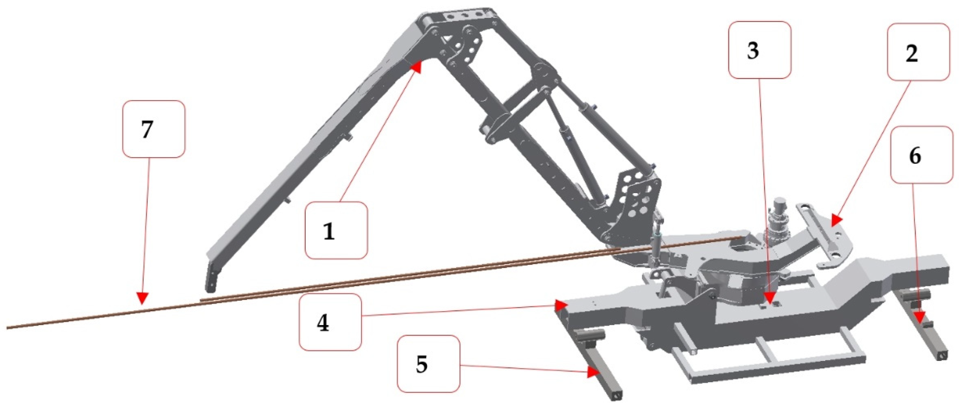
The manufacturer of the harvester provided an incomplete 3D model consisting of a complete crane set, an incomplete slewing platform without a cabin, a complete tilting bottom plate of the slewing gear, and an incomplete (schematic) machine frame (Figure 2). The reason for not delivering the full model was the protection of intellectual property. To be able to carry out the simulation, it was necessary to make a schematic model of the axles, which have a significant function in the simulation (Figure 2, pos. 5 and 6). Both axles (front, rear) were modelled based on visual documentation with similar parameters in terms of weight and dimensions. The remaining components of the machine that were not provided were replaced in the MSC Adams programme by point masses found in catalogues or using information provided by the manufacturer. When preparing the dynamic model for the simulation, it was necessary to first create in a 3D model maker functional systems of moving units which consist of several components or break down the system into moving subsystems. The weight of the functional model system could be validated using the real machine and portable vehicle scales on which the machine was weighed before the verification during a field investigation. In total, 22 functional component systems were created for the AH6 harvester model with mutual motion connections as in reality.
2.2.2. Coordinate System
Before exporting the functional component systems and the measuring instruments (Figure 2, pos. 7) to the import files for MSC Adams, it was necessary to place the entire system of the AH6 harvester 3D model in the 3D CAD (Computer aided design) coordinate system based on the need to evaluate the dynamic analysis results. The 3D CAD coordinate system is hereditary for the MSC Adams simulation programme. If the model was slightly rotated with respect to the central coordinate system, the dynamic analysis results would have to be added as vectors in the axes, which would generate errors in the verification of values in relation to the experiment [13]. For the export from 3D CAD, and thus for the simulation as well, it was necessary to establish the direction of the main coordinate system and the origin of the coordinate system, to adhere to it, and use the same terminology in the simulation and in the experiment. The main coordinate system and the origin of the coordinate system were established as follows:
The +X axis direction in front of the harvester (the longitudinal axis of the harvester undercarriage in the forward direction). The +Y axis towards above of the harvester (perpendicular vertical direction of the harvester, direction -Y is the direction of the gravitational acceleration). The +Z axis is the direction from the longitudinal axis to the right of the harvester. The coordinate system directions are apparent from Figure 3 The origin of the 3D model coordinate system was placed in the intersection point of the axis of the tilt pin of the harvester slewing gear and the longitudinal axis of the machine (lies in the same plane as the axis of the slewing gear), see Figure 3. This location was selected to enable the control of the tilt and the position of other measured points in relation to this fixed point with respect to the structure of the harvester.
After establishing the coordinate system of the AH6 harvester model and its positioning for the origin of the coordinate system in 3D CAD, each functional component was exported to export “binary Parasolid” files with the *.x_b extension. This 3D model format has several advantages such as the heredity of the coordinate system, orientation, low demands for graphic display and file size compared with other types of file that can be imported into the simulation programme [21].
2.3. Adams—The Numerical Simulation Model
When importing the 3D model components into the MSC Adams simulation programme, it was not necessary to pay attention to any marginal conditions or measuring scales thanks to a thorough preparation of the components exported [13,27]. The 3D model components became the numerical model units. Particularly, the numerical simulation model consists of 22 moving components (Figure 4).
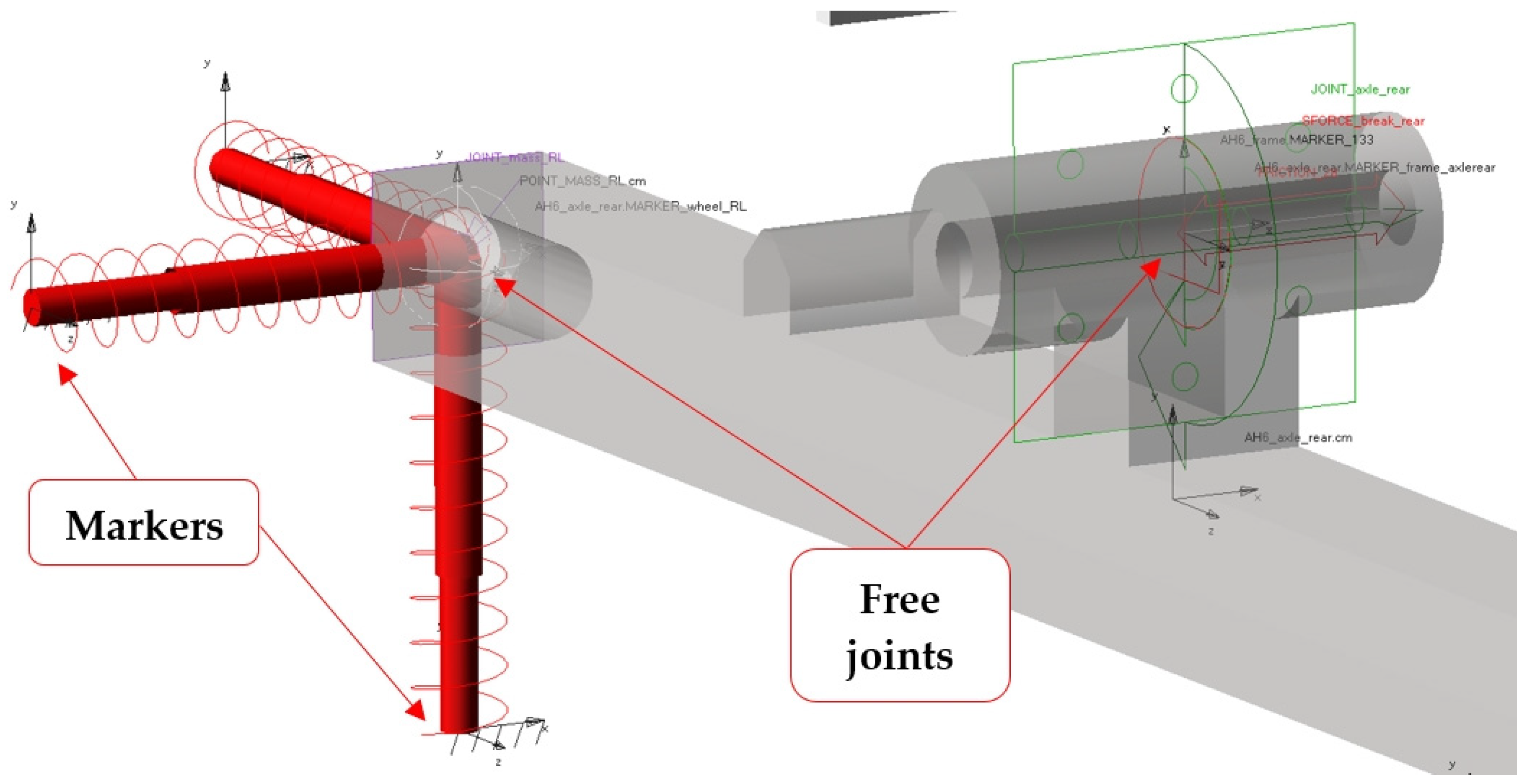
A so-called marker was created for each component placed in reference locations of joints, hinges, or other locations related to the ties with other components. The creation of the markers was primarily based on the geometric shape of each component and, hierarchically, a marker belongs to the component it has been assigned to [21]. Each individual marker keeps its position in relation to the component. During the simulation, it was possible to observe the shift (trajectory) or the movement (speed, acceleration) of the marker when being placed in the component (see Figure 5). Another property of the marker is that a moving joint between the numerical model components can be placed in its coordinate position. This made easier the work related to binding the components with respect to their function in the dynamic system.
2.3.1. Joints between the Components
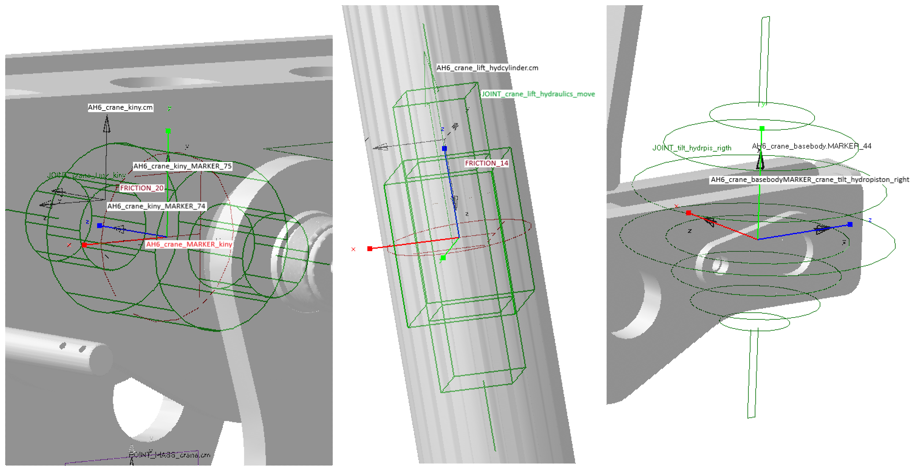
A total of 28 moving joints between the components were created on the numerical model, two of which were cylindrical joints, 16—revolute joints, five—spherical joints, and five—translational joints (Figure 5).
Two cylindrical joints were created between kinematics X and kinematics Y of the loading crane (Figure 6) and between kinematics 1 and kinematics 2 (Figure 6) of the loading crane near the control cylinders. This type of joint was used because, considering the kinematics design, the statistical determination of the joint system had to be preserved. Five translational joints were created mainly between the components between which there is translational movement (Figure 6). A secondary reason was preserving the statistical determination of the related joint system. All the five translational joints were used in the piston–piston rod joint in all the five cylinders, i.e., two for controlling the loading crane, one for tilting the slewing platform, two for tilting the crane at the base (Figure 6). Five spherical joints were created only for hydraulic pistons. More precisely, it is a joint fixing a hydraulic piston to the pivot of the mechanism (Figure 6). The reason was again the preservation of the statistical determination of the related joint system of the cylinder mechanism.
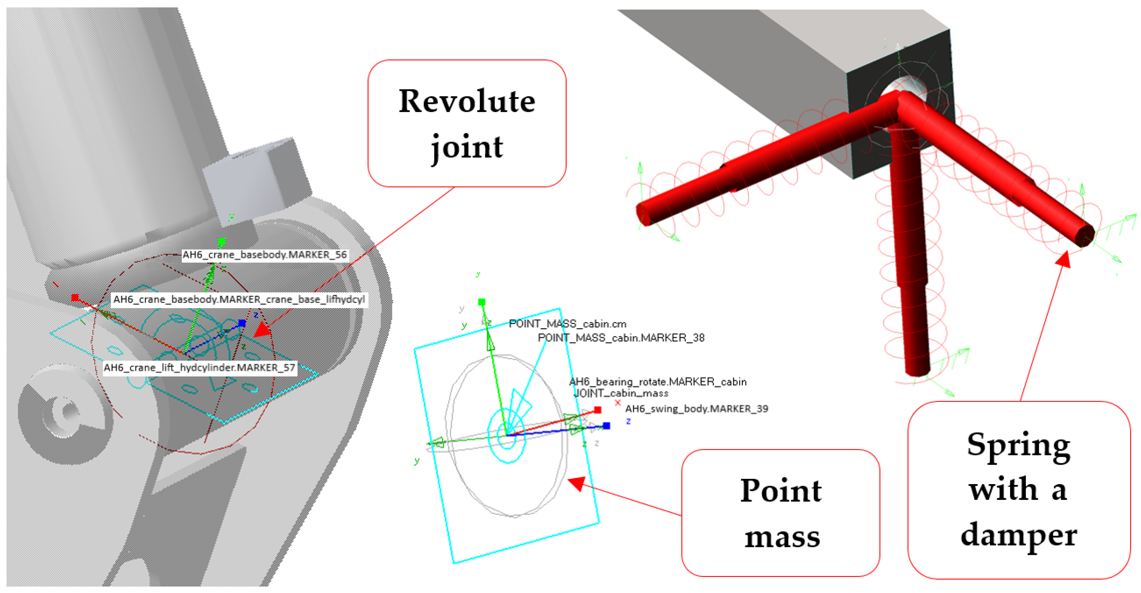
The prevailing type of joints used for the numerical model mechanisms is the revolute joint, which has the same properties as the revolute joint, i.e., one rotational degree of freedom; the other translational and rotational degrees are blocked. The number of the revolute joints used was 16 for all the other rotary moving components as a substitute for the revolute joint (Figure 7) [28].
In the next step of the numerical model, markers were created at reference points on which point masses were subsequently created to add weight to the incomplete model (Figure 7). The centre of gravity of the other components was assumed at these points, and their weight was derived from the values obtained in the field research on the experimental prototype. To reach the operating weight of the machine, eight point masses were used. Four point masses were used for the cabin, the machine (accumulators, hydroelectric generating sets, etc.), the crane (the hydraulics, small components), a substitute for the harvester head and hydraulic rotator. Furthermore, four point masses were located at the ends of the axles where the wheels were fixed (Figure 7). Weight was added to the wheels based on the data obtained in the field research.
2.3.2. Types of Attachment of the Dynamic System
The AH6 prototype belongs to the class of small-size wheeled harvesters [10]. The chassis frame is fitted with two swinging axles whose transverse slope and blocking can be controlled. The MSC Adams programme enables the modelling of simulation tasks using tyres that are part of the libraries and solvers in the programme in terms of the model and calculation [21]. Their usage in the model was quite unstable in the first simulation attempts and caused some solutions to finish prematurely due to the loss of stability. This is why the whole simulation numerical harvester model was built upon elements such as a spring and a damper instead of the simulation element of a tyre (Figure 7) [29]. The whole dynamic system then became stable. When a wheel was lifted and the contact with the ground broken, the solver calculation was not interrupted. However, the simulation calculation detected the opposite effect and it was possible to assess the behaviour of the system although both the dynamic action and the condition were impossible in reality [19,23,26,29].
Each of the harvester tyres was replaced by three springs and dampers whose parameters corresponded to the strength and damping in the axis. The reference spring and damper were on the Y axis representing the vertical properties of the tyre. The parameters were defined based on the type of tyre and pumping, on the previously established parameters, and the parameters in the element library of the MSC Adams programme. The strength was determined based on the theory of Wong [30] as k = 2810 N·mm−1 and the damping as b = 100 N·s·mm−1 for the vertical direction of the tyres. For the horizontal direction of the tyres, the strength was determined as k = 2000 N·mm−1 and the damping as b = 100 N·s·mm−1. The horizontal direction of the tyres has a stabilizing effect on the model, and their reduced value, in relation to the vertical direction, corresponds to the function of the tyres in transverse directions [13,22,26].
2.4. Validation of the Experiment
2.4.1. Determining the Lifting Torque
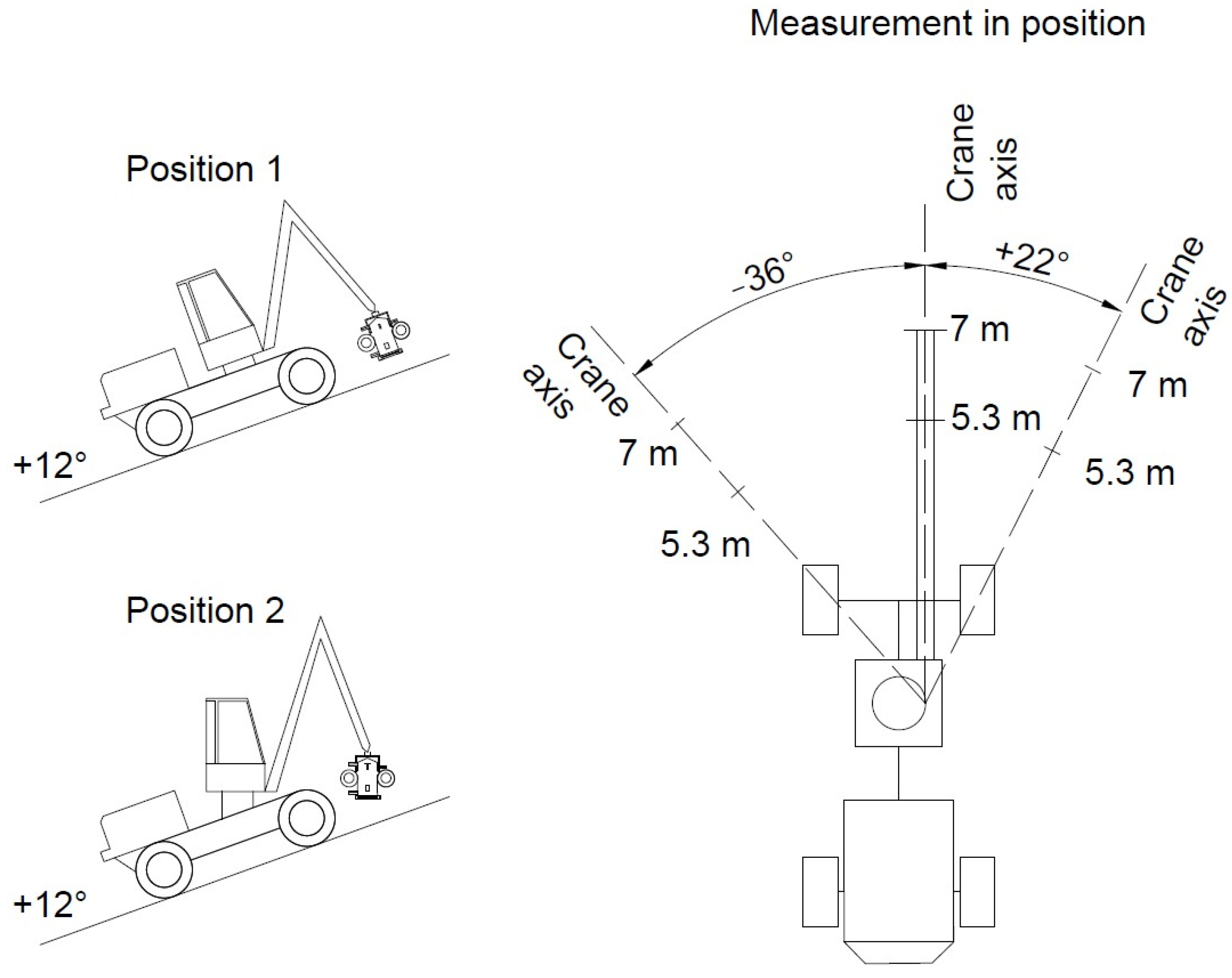
To validate the results, the AH6 harvester was placed in two different positions. Specifically, in position 1, it was on a +12° slope (operating up the slope), and the slewing gear was not levelled, which means it was tilted backwards at −12°. In position 2, the machine operated on the same slope as in the previous position; however, its slewing gear was levelled with the horizontal plane, i.e., making an angle of 0°. Both the positions are shown in Figure 8. In each position, six ground control points were defined on three axes (one axis, two points), where the reference axis (0°) was parallel to the longitudinal axis of the machine and another axis formed an angle of −36° with it, so it was an axis located to the left of the longitudinal axis (Figure 8). The third, last, axis formed an angle of +22° with the longitudinal axis of the crane; thus, the axis was on the right. On each of these axes, two points were marked. The first one was 7 m away from the axis of the slewing gear and the other one was 5.3 m away from the same axis. The measurement was then performed at the thus defined points, see below.
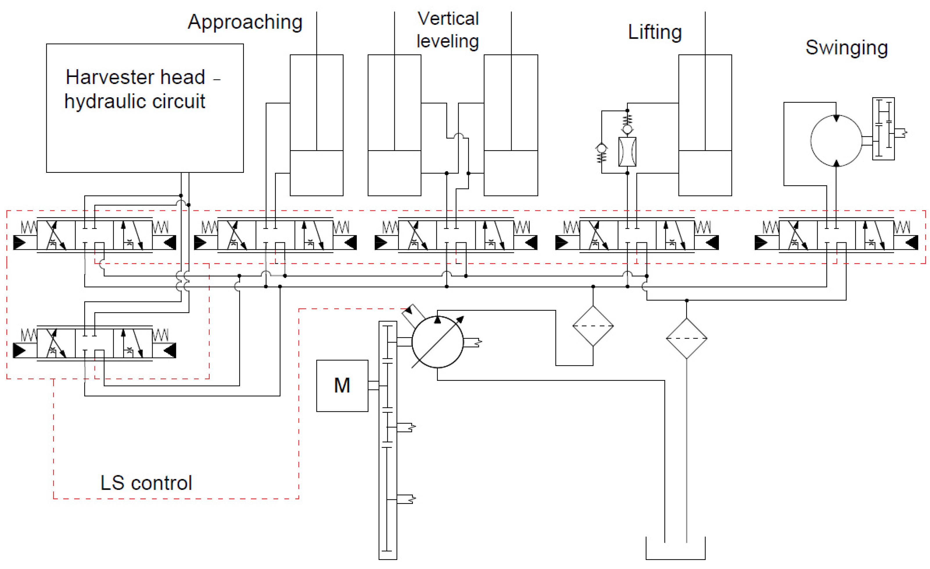
To validate the dynamic analysis and thus answer the question about the lifting torque, it was necessary to enter the maximum values of the force acting on the end of the hydraulic crane during lifting and weight down the wheels to balance the model. For this purpose, field research was first carried out including the previously defined positions and ground control points. In the first step, the loading of each wheel was measured at the given ground control points on the axis parallel to the longitudinal axis of the machine (further on also referred to as 0°). Dini Argeo DFWKR portable vehicle scales by Dini Argeo with a loading capacity of 8000 kg were used for this purpose. After acquiring the data on the loading of each wheel, a measurement was performed of the maximum force that the crane is able to exert in the given distances when lifting a load. The forces were recorded using a U2A tension and compression load cell by Hottinger Baldwin Messtechnik GmbH, which can measure a load of up to 5 tons. The tensometer was attached to the suspension joint of the hydraulic crane by a textile cord with a strength of 5 tons so the harvester head frame could not be damaged by an excessive load. The tensometer was also attached to a fixed anchor on the ground by a textile cord with the same strength. Subsequently, five attempts were made to exert the maximum lifting force of the crane at each point. The forces detected were also used in the dynamic analysis, which made it possible to calculate the pressure at the theoretical level necessary to exert the given force. The theoretical results yielded by the dynamic analysis were then verified in practice since the hydraulic system was monitored during the measurement using a HySense QT 100 turbine flowmeter and a MultiHandy 3020 data logger by Hydrotechnik GmbH. The measurement frequency was 33 Hz. The flowmeters were placed in the open hydraulic circuit of the crane. A flowmeter was installed between the hydraulic switchboard and the lifting cylinder of the crane (see Figure 9). Specifically, it was attached to the branch in which fluid ran during the attempt to exert the maximum lifting force affecting the torque theorem. For the purposes of the measurement, the one-way flowmeter had to be protected from getting destroyed by the down-pressure check valves using a spring. The valves used a safety pressure of 1 bar.
2.4.2. Determining the Slewing Torque
Besides investigating the dependence of the lifting torque of the crane and the slewing gear slope, including the subsequent comparison of the hydraulic pressures in the MSC Adams programme, a comparison was also made of the slewing torque size with the slewing gear levelled and not levelled. This means that the same model was used with the same positions and distances of the ground control points from the axis of the slewing gear as for the lifting torque. Considering the problems observed in relation to the stability of the machine and safety of the operator during the operation tests, this research remained at the theoretical level. Therefore, to verify this, only a dynamic analysis of the crane was used, in which, instead of the given torque, the surface resistance that had to be overcome for the crane to move was monitored for each component in and out of the slewing bearing. The torque values then correspond to the inverse resistance values.
The theoretical determination used, as has already been mentioned, the distances given for the reach of the crane and the positions as in the measurement of the lifting torque. However, in this case, the axes were not used. For the purposes of the research, only the maximum slewing angle of the slewing gear was defined, which was ± 105°. This slewing angle was marked by electrical sensors but the end maximum slewing angle was actually ± 110°, which was determined by mechanical stops. This is why the slewing angle of the slewing gear selected in the dynamic analysis was ± 108°.
The actual measurement was performed as follows. Besides the weight of the head, the load was also included in the suspension joint. At a distance of 7 m, a 300 kg load was selected, and in each of a total of five attempts, 20 kg were removed. The same was true at a distance of 5.3 m, but the starting weight here was 500 kg. The loaded crane was always moved to the starting position, which was at −110° (on the left). Then, it was rotated to +110°, and then the crane returned to the starting position. After the crane was stopped at −110°, the weight of the load was reduced and the whole process was repeated. It should be added that, for the measurement, only the slewing angle of ±108° was monitored since, in this section, the rotation speed was constant the entire time.
2.5. Statistical Analyses
The sections of interest to the research were selected from the datasets acquired. They were the data sections related to the exertion of the maximum lifting force of the crane or the rotation of the crane with a given weight within the range of ±108°. Specifically, a comparison was made of the data obtained during the field research and from the dynamic analysis at the same points and positions of the machine when measuring the lifting cylinder of the hydraulic crane. It was also investigated whether the lifting and slewing torques of the crane were affected by the slope of the slewing bearing. To evaluate the data correctly, the Shapiro–Wilk test was performed with the level of significance p (further on also referred to as the p-value) being 0.05. If the result of the dataset tested was greater than this selected value, the data were, according to Student’s distribution, regarded as normally distributed, and vice versa.
If two sets were compared whose data were normally distributed, the test performed subsequently was the t-test. If one of the sets being compared contained abnormally distributed data, the Mann–Whitney U test was performed. The same statistical test was also performed if all the sets being compared contained abnormally distributed data. The level of significance was established at 0.05, the same for all the tests. The datasets were not different if the result of the statistical analysis exceeded the p-value specified.
The data obtained by measuring the slewing torque of the crane, more precisely, the values of resistance in the slewing gear during the rotation of the hydraulic crane, were subjected to a regression analysis. The aim of this test was to verify whether the resistance in the slewing mechanism when its slope is −12° is affected by the angle formed at that moment by the crane rotating from left to right and back in relation to the longitudinal axis of the machine. First, the data for each movement were plotted in a scatter plot, which was then used to evaluate the linear regression function, and the coefficient (index) of determination designated by R2 was calculated showing the level of quality of the regression model. If it is 1, the prediction can be made with a confidence of 100%. However, if the result is 0, the regression model and its precision will have a 0% confidence.
3. Results
3.1. Lifting Torque of the Crane
The field research investigated the maximum lifting force a hydraulic crane can use with the reach distances being 7 and 5.3 m and the slewing bearing being levelled and not levelled. The results are shown in Table 1.
Table 1 shows an apparent difference in the maximum forces used when the slewing bearing is in the horizontal plane (0°) or copies the slope but in relation to its axis, the value is negative, i.e., not +12° but −12°. It is quite apparent, even from these data, that the slope affects the lifting torque in favour of the slewing gear not levelled. This statement has been verified by statistical analyses showing that the tilt of the slewing gear affects the lifting torque of the hydraulic crane since all the values shown in Table 2 were lower than the specified level of significance (0.05).
After a basic statistical description of the maximum force exerted by the hydraulic crane at the given reach distances and with the given slope of the slewing gear and axis, it was found that the average difference on the −36° axis (i.e., the one above the front left wheel of the machine) at the reach of 5.3 m was 2212.38 N in favour of the slewing gear with a slope of −12°. However, at 7 m on this axis, it was the opposite. The difference here was only 390.30 N in favour of the levelled slewing gear. The same result was obtained on the 0° axis both at the reach of 5.3 m and 7 m. A greater force was detected here, always with the slewing gear with a slope. Specifically, the difference at 5.3 m was 2712.52 N, and only 441.30 N at 7 m. The last axis on which the maximum force that the hydraulic crane can exert was measured was the +22° axis. On this axis, the result of the comparison of forces was identical to that on the −36° axis, i.e., at the distance of 5.3 m, the crane exerted a greater force with the slewing gear being at −12°, and at 7 m, it was the other way around. The difference between the slewing gear levelled (0°) and at the angle of −12° was 2270.24 N at 5.3 m and 358.92 N at 7 m.
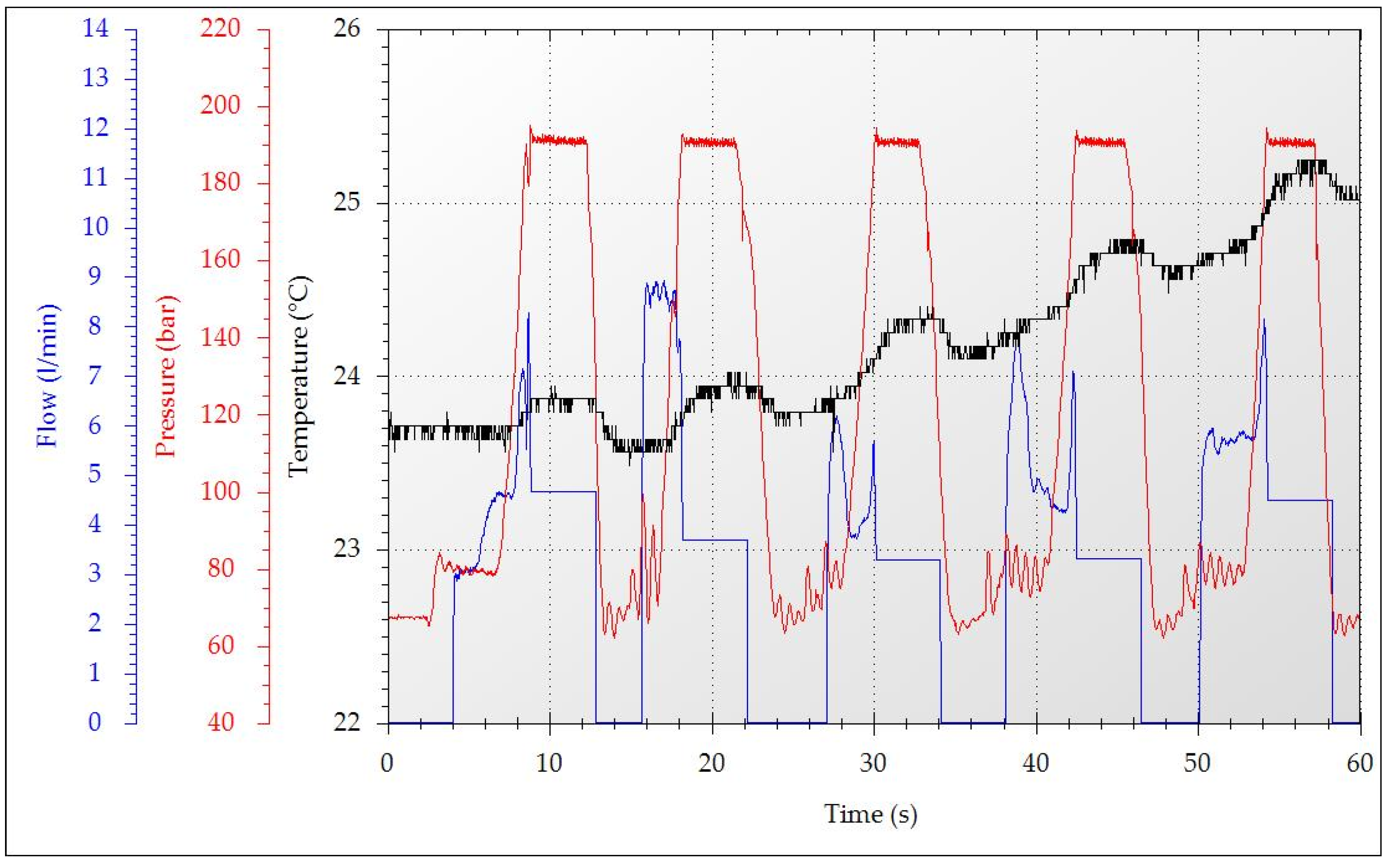
When measuring the maximum force possible that the hydraulic crane can exert, a flowmeter recording the data from the hydraulic circuit during the measurement was attached to the cylinder enabling the lift of the crane. Since the set of the data from all the measurements was very large, this paper only presents the data for the point of 5.3 m on the 0° axis, which fully represents the results obtained. Figure 10 shows the flow, pressure, and temperature of the hydraulic oil during the measurement on the 0° axis at the point 5.3 m distant from the centre of the slewing gear positioned at the angle of −12°. Five pressure peaks can be observed. They are sections in which the maximum force of the crane was measured. The first peak corresponded to the force in Measurement 1 (Table 1).
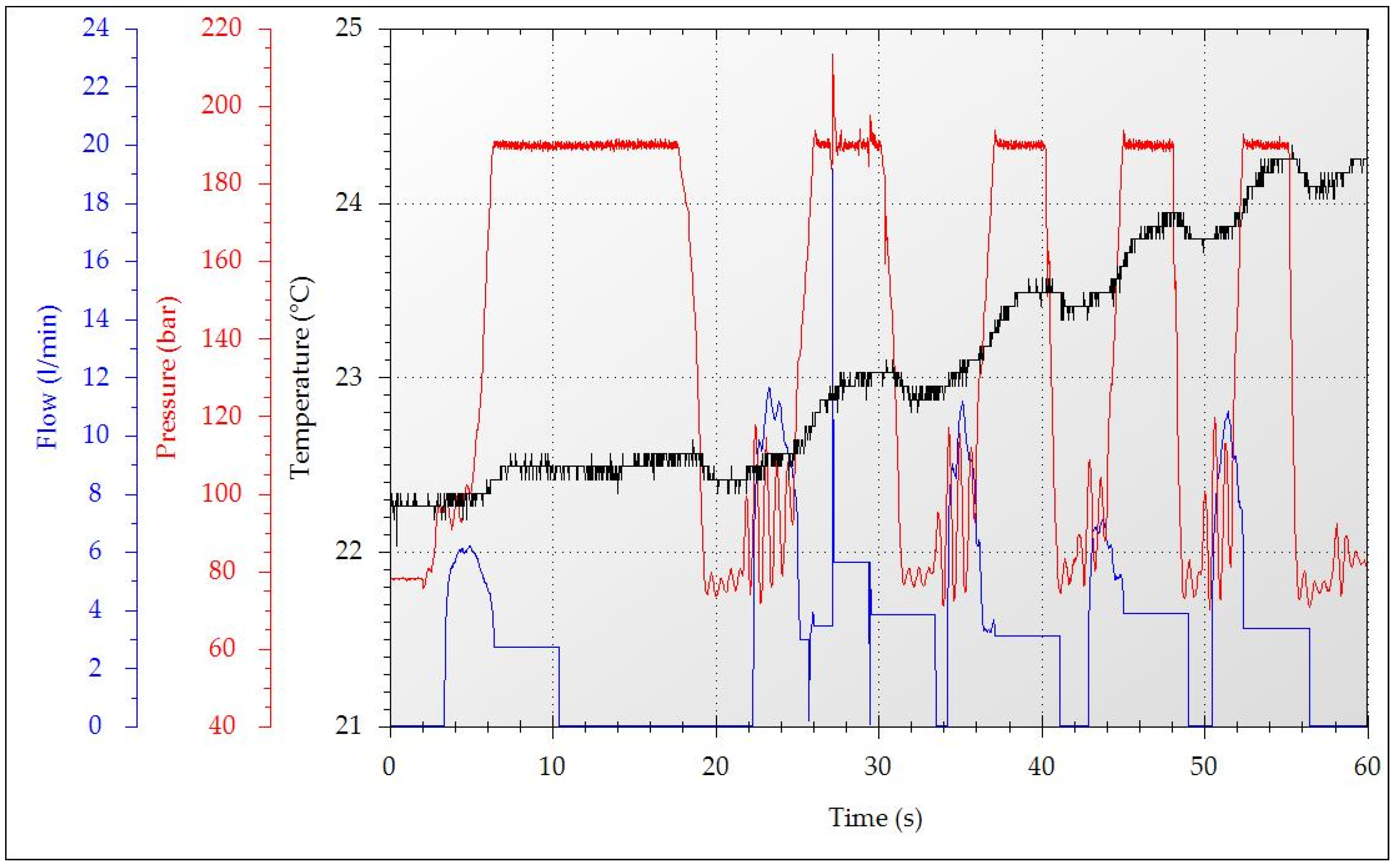
The average hydraulic pressure when measuring on the 0° axis at the 5.3 m point with the slewing gear not levelled (−12°) was 190.71 bar. The maximum pressure was reached at 8345.46 N. It was the first peak out of five. Its value was 194.85 bar, which was 5.76 bar more than the pressure minimum. The most frequently reached pressure value was 190.58 bar. At the same point and on the same axis but with the slewing gear levelled (Figure 11), the average pressure reached was 190.05 bar, which was almost the same as when the slewing gear was at −12°.
Figure 11 shows a high maximum pressure (213.25 bar) in the second measuring attempt. Such high pressure is preceded by a very high flow reacting to a decrease in the pressure to 183.70 bar, the minimum value recorded. This divergence, lasting only 0.30 s, can be explained by the function of the directional valve, where the hydraulic spool could have been disengaged from its position or the control signal voltage could have dropped. Such an occurrence was very rare during the measurement. Overall, it can be stated that the same pressure was reached in both the positions of the slewing gear but the maximum forces of the crane were different.
The trend detected during the field research related to the hydraulic circuit was verified by a dynamic analysis in the MSC Adams software, where the same maximum forces recorded in the field research were entered and the pressure acting on the specific part of the cylinder piston was calculated. Figure 12 shows the pressure condition for each of the forces acting in the simulation on the 0° axis at the 5.3 m point with the slewing gear not levelled (−12°). When comparing the pressure with Figure 10, it is apparent that with the force being the same, the pressure is different, which confirms the result of the statistical test in Table 3. Based on the calculation made by the programme, the pressure of 183.73 bar was needed to exert the particular forces, which is 6.98 bar less than what was measured. The maximum pressure provided by the calculation was 186.86 bar and the minimum was 181.71 bar. The most frequently calculated value was 183.55 bar.
Figure 13 shows the theoretical behaviour of pressure at the 5.3 m point on the 0° axis with the slewing gear levelled (0°). Again, in comparison with the field measurement (Figure 11), a difference between the pressures is apparent. This is also confirmed by the result of the statistical analysis in Table 3. The average pressure, according to the dynamic analysis, was 154.54 bar. Thus, the difference was 35.50 bar in comparison with the measurement. The maximum pressure calculated in the simulation was 158.45 bar and the minimum was 151.87 bar. The most frequently reached pressure value was 154.46 bar.
When comparing the field measurement and the dynamic analysis, their percentage difference was monitored, which is shown in Table 4. The smallest differences, and thus the highest precisions, at the 5.3 m point occurred on the 0° axis with the slope of the slewing gear being −12° (parallel to the slope of the ground). The model and reality only differed at this point by 3.66%. In contrast, the highest inaccuracy, 23.50%, was observed on the −36° axis with the slewing gear levelled (0°). Furthermore, at the 5.3 m distance, a certain trend could be noticed of higher inaccuracy between the model and the reality, always with the slewing gear at 0°. The total deviation at the given distance was then 14.64%.
The smallest difference at the 7 m distance was 0.23%, which was on the +22° axis with the slewing gear making an angle of −12°. The highest inaccuracy between the model and the reality occurred in the pressure values recorded on the axis parallel to the longitudinal axis of the machine (0°) with the slope of the slewing gear being 12°. Specifically, the difference here was 7.88%. At the 7 m distance, the same trend could be seen as at 5.3 m, except for the 0° axis, on which the differences were almost identical. The total inaccuracy at 7 m was only 5.01%, which is 9.63% less than at the 5.3 m distance. Overall, the dynamic analysis data differed from the real measurement by 9.82%.
3.2. Slewing Torque
In addition to the research on the dependence of the lifting torque of the crane and the slope of its slewing gear, including the subsequent comparison of the hydraulic pressures in the MSC Adams programme, a comparison was also made of the slewing torque with the slewing gear levelled and not levelled. Considering the issues related to the centre of gravity of the machine when the hydraulic crane is rotating, a field investigation could not be carried out for safety reasons. The results of the initial experimental field measurements proved the instability of the prototype AH6 machine, which was also confirmed by simulations. Therefore, only a dynamic analysis of the crane was performed. Instead of the given torque, this analysis monitored the surface resistance that had to be overcome for the crane to move each component in and out of the slewing bearing. The torque values then correspond to the inverse resistance values.
Figure 14 shows the development of the resistance while the crane with the slewing gear levelled is moving from left to right and back with a reach of 5.3 m. When the angle was negative, the crane was on the left side of the machine from the driver’s point of view. If the angle was positive, the crane was on the right side. The 0° axis was the axis of the crane parallel to the axis of the machine (as in the other measurements). The negative resistance values conformed to the same rule as the angles, only with inverse signs. However, in terms of a comparison of the left and right sides, they could be regarded as positive in all the cases. This rule also applied to the speed. Considering the large amount of data, only the measurement at the distance of 5.3 m from the axis of the slewing gear is presented.
Figure 14 clearly shows an even resistance throughout the rotation of the hydraulic crane from left to right and back at a constant speed, i.e., in the range from −108° to +108°. In the first rotation cycle, the crane was weighted, besides the weight of the rotator and the harvester head, at its end, which was 5.3 m away from the centre of the slewing gear, using a 500 kg load. In each of the following four cycles, the load was always reduced by 20 kg.
The average resistance that had to be overcome and was calculated during the movement from the angle of −108° to 0° was 5762.63 Nm. During the subsequent movement from 0° to +108°, it was 5751.61 Nm. As the crane was returning from +108° to 0°, it was determined to be −5753.99 Nm. The resistance detected from 0° to −108° was 5761.25 Nm. These are very even values of friction in opposing motion. Specifically, the differences only ranged from 437.20 Nm up to 551.90 Nm. The same trend of even resistance with the slewing gear levelled was also observed at the 7 m distance.
Figure 15 shows the development of resistance when the slope of the slewing gear was −12°, the reach of the crane was 5.3 m, and the load was the same as with the slewing gear levelled. It is quite obvious that it is affected by the slope, which was also confirmed at the 7 m distance. When the crane was moving from the angle of −108° to 0° (i.e., ascending), the average resistance was 5523.71 Nm. After crossing the zero angle towards +108°, an opposite situation occurred when the crane was descending. The average resistance during the descent was 5538.87 Nm. In the opposite case, when the crane was rotating from left to right, the average resistance during the ascent was 5540.82 Nm. During the descent, this value was −5519.60 Nm.
It is quite evident even from these data that the resistance is affected by the slope of the slewing gear, which is also confirmed by the result of the statistical tests comparing the distances of 5.3 m and 7 m, which was <0.001. The level of significance was 0.05; therefore, the dependence of the slewing torque (resistance) and the position of the slewing gear were ascertained. However, what must also be considered is the angle at which the crane operates at the given moment since, when the crane gets closer to the 0° axis, the slope gradually decreases, and vice versa. This is why for each movement from one side to the other, a regression model was made to plot the dependence (Figure 16).
Figure 16 shows a detailed view of the first movement of the crane from −108° to +108°. The blue dots are data from the dynamic analysis. After their display, a parabolic regression function was selected based on their distribution. After the basic equation was calculated, the coefficient of determination (R2) was also evaluated. Its value and the parabola equation can be seen in Figure 16 (the parabola is marked in red). In this case, the coefficient was 0.9848, which means that the parabola represents, with a precision of 98.48%, the resistance values that must be overcome when the crane rotates from left to right with a 500 kg load. The other movements repeated in the measurements with a different load suggested that the overall parabolic regression function at the 5.3 m reach corresponded with a precision of 98.32% (R2 = 0.9832). The same trend in the resistance of the slewing gear not levelled and the regression function was also detected at the 7 m distance, where the maximum load weight was 300 kg (20 kg less in the next movement). The average coefficient of determination in this case was 0.9645, which means that the shape of the parabola corresponded to the resistance with a precision of 96.45%. The graphical solution and the numerical values cannot be published here due to the large amount of the data.
After the parabola is plotted (the red dots), Figure 16 clearly shows the dependence of the resistance and the angle at which the crane operates, which, to a certain extent, confirms the dependence on the position of the slewing gear. Overall, the behaviour of the resistance that must be overcome for the crane to rotate up and down a slope corresponds, in terms of shape, to a parabola with a precision of 97.38% (R2 = 0.9738). This suggests that the slewing torque of a hydraulic crane corresponds to a parabola inverse to the resistance, and therefore the relations confirmed for the resistance also apply to it. If the slope of the slewing gear is −12° (tilted backwards) when the crane moves up a slope, the slewing torque is smaller than when the crane is levelled. The largest values of the torque are reached in front of the machine, i.e., at the 0° axis.
4. Discussion
Currently, the CTL technology is used increasingly often on previously inaccessible sloping grounds, which has been shown by many studies [1,2,3,4]. Its employment increases the work safety [6,7]. According to Visser and Stampfer [1], these machines are equipped with the option of levelling the hydraulic crane and cabin, which enhances the operating ergonomics and makes the machine more stable. Levelling the crane with a cabin, or more precisely their slewing bearing, affects the productivity, according to the empirical studies conducted by Schiesse et al. [11]. These statements about the productivity, stability, and ergonomics of the machine can be, by virtue of the results presented in this paper, considered incomplete but not incorrect.
The results confirm a relation between the lifting torque of a hydraulic crane and the slope of the slewing gear. Specifically, when operating up a slope not being levelled, it reaches higher lifting torque. However, the slewing torque is lower, or rather, it behaves 97.38% parabolically, where the vertex of the parabola corresponds to the maximum value detected in front of the machine (i.e., on the 0° axis). The minimum is then located the furthest from the 0° axis. In this case, the minimum was detected at the angle of ±108°, where the speed was constant. Considering the data acquired, it can be stated that: “Levelling the slewing gear of a hydraulic crane primarily maintains the force characteristics it has in a horizontal position and, secondarily, the operating ergonomics and the machine stability are maintained.” What can also be taken into account is the rationalization of the structure of the crane, which makes it possible to level the slewing gear.
When measuring the lifting torque and the maximum force it can exert, the hydraulic pressure and its flow were also monitored. It was found that the pressure, within the slope of the slewing gear of the crane, remains the same unlike its maximum lifting force. Subsequently, after substituting the maximum forces measured into the dynamic analysis of the lifting torque, pressure value differences were detected between the slewing gear levelled and not levelled as well as between the field research and the model. Table 4 shows the average pressures at the specific distances and on the selected axes. For example, on the 0° axis, with the slope of the slewing gear being −12°, it was 183.73 bar and, with the slewing gear at 0°, it was 154 bar. With this lower pressure value, a weaker force was exerted ranging from 2530.12 to 2892.96 N. However, in the field research, with the slope of the slewing gear being −12°, the pressure was 190.71 bar and, with a slope of 0°, it was 190.05 bar. A comparison yielded a difference of 3.66% with the slewing gear being at −12° and 18.68% when the slewing gear was in a horizontal position (0°).
The small difference between the model and the measurement with the slope of the slewing gear being −12° could, to a certain extent, be accounted for by the resistances in the hydraulic circuit since the software only works with the pressure it calculates from the known area of the hydraulic cylinder and does not include the hydraulic fluid. However, this explanation does not apply to a deviation of 18.68%. Therefore, a question should be asked what has caused this deviation and why was it not also detected at the 7 m distance. The answer could be provided by a more long-term research. If, even despite these inaccuracies, the total deviation was determined to be only 9.82%, it can be said that using a dynamic analysis to determine the basic lifting torque is appropriate but a deviation of up to 10.00% must be expected. This deviation could theoretically be improved by adding more numerical calculations and refining the boundary conditions as the field survey can have many factors that cannot be predicted in the simulation. The question for further research is also whether increasing the numerical calculations will not increase the deviation.
5. Conclusions
Overall, it can be stated that levelling the slewing gear of a crane is necessary on a sloping ground, especially since the effect on the lifting and slewing torques is reduced. It has been found that when the slope of the slewing gear is −12°, the lifting torque reaches a higher maximum lifting force than when the slewing gear is in a horizontal position (0°). The research has confirmed a relation between the slope of the slewing gear and the lifting torque. As part of the theoretical verification by a dynamic analysis of the crane and the AH6 machine, a different pressure was detected in the lifting cylinder compared to the field research. The total deviation of the simulation from the field research was 9.82%, which can be considered acceptable; however, it must be taken into account when designing lifting loaders.
The paper was also concerned with determining the effect of the slewing bearing slope on the slewing torque. The research has shown that, with the slewing bearing not levelled, the slewing torque can be characterized 97.38% by a parabola, whose vertex is located in front of the front part of the machine and goes down when the crane moves to the left or right. It follows that when the crane is not levelled and is moving up a slope from left or right, the slewing torque is significantly lower than with the crane levelled. Overall, it can be determined that, when the crane is rotating up a slope, whether it is from left or right, the slewing torque is lower and it increases as the crane gets closer to the front of the machine (along the longitudinal axis of the machine). The behaviour of the slewing torque is then characterized by a parabola.
The results of the research show the necessity to equip hydraulic cranes with CTL technology because of the growing trend of them being used on sloping grounds. Levelling the lifting equipment is the only way of reducing the force and torque load, which is a promising aspect to the integration of levelling into CTL technology machines and their automation or programmability with regard to the operating conditions of the machine. Levelling reduces the weight of some parts of the machine bringing down the energy consumption with additional ergonomic benefits for operation. In the future, the force and torque parameters can be calculated in advance using numerical models in software of the MSC Adams type.
Author Contributions
Conceptualization, V.M. and J.K.; methodology, V.M.; software, V.M. and J.K.; validation, V.M.; formal analysis, V.M. and J.K.; investigation, V.M. and J.K.; resources, V.M. and J.K.; data curation, V.M.; writing—original draft preparation, V.M. and J.K.; writing—review and editing, V.M. and J.K.; visualization, V.M. and J.K.; supervision, J.K.; project administration, J.K.; funding acquisition, J.K. All authors have read and agreed to the published version of the manuscript.
Funding
This work was supported by the specific research on BUT FSI-S-20-6267.
Institutional Review Board Statement
Not applicable.
Informed Consent Statement
Not applicable.
Data Availability Statement
The data presented in this study are available in the article. Additional data are available on request from the corresponding author.
Acknowledgments
The authors gratefully acknowledge funding from the specific research on BUT FSI-S-20-6267.
Conflicts of Interest
The authors declare no conflict of interest.
References
- Visser, R.; Stampfer, K. Expanding Ground-based Harvesting onto Steep Terrain: A Review. Croat. J. For. Eng. 2015, 36, 321–331. [Google Scholar]
- Visser, R.; Berkett, H. Effect of terrain steepness on machine slope when harvesting. Int. J. For. Eng. 2015, 26, 1–9. [Google Scholar] [CrossRef]
- Enache, A.; Kühmaier, M.; Visser, R.; Stampfer, K. Forestry operations in the European mountains: A study of current practices and efficiency gaps. Scand. J. For. Res. 2016, 31, 412–427. [Google Scholar] [CrossRef]
- Cavalli, R.; Amishev, D. Steep terrain forest operations—challenges, technology development, current implementation, and future opportunities. Int. J. For. Eng. 2019, 30, 175–181. [Google Scholar] [CrossRef]
- Axelsson, S.Å. The mechanization of logging operations in Sweden and its effect on occupational safety and health. Int. J. For. Eng. 1998, 9, 25–31. [Google Scholar] [CrossRef]
- Bell, R.K. Changes in logging injury rates associated with use of feller-bunchers in West Virginia. J. Saf. Res. 2002, 33, 463–471. [Google Scholar] [CrossRef]
- Raymond, K. Innovative Harvesting Solutions: A Step Change Harvesting Research Programme. N. Z. J. For. 2010, 55, 4–9. [Google Scholar]
- Ghaffariyan, M.R.; Acuna, M.; Ackerman, P. Review of new ground-based logging technologies for steep terrain. CRC For. Bull. Hobart Tasman. Aust. 2012, 21, 1–5. [Google Scholar]
- Jodłowski, K.; Kalinowski, M. Current possibilities of mechanized logging in mountain areas. For. Res. Pap. 2018, 79, 365–375. [Google Scholar] [CrossRef] [Green Version]
- Neruda, J. Harvestorové Technologie Lesní Těžby, 1st ed.; Mendel University in Brno: Brno, Czech Republic, 2013; pp. 1–165. [Google Scholar]
- Schiess, P.; Schuh, D.; Miyata, E.S.; Mann, C.N. Concept Evaluation of a Walking Feller-Buncher—The Kaiser X5M Spider Concept Evaluation of a Walking Feller-Buncher—The Kaiser X5M Spider. In Proceedings of the 1st Technical Conference on Timber Harvesting in the Central Rockies, Ft. Collins, CO, USA, 4–6 January 1983; pp. 40–52. [Google Scholar]
- Amishev, D.; Evanson, T. Innovative methods for steep terrain harvesting. In Proceedings of the FORMEC 2010 Forest Engineering: Meeting the Needs of the Society and the Environment, Padova, Italy, 11–14 July 2010; pp. 1–9. [Google Scholar]
- Omar, M.A. Modeling and simulation of structural components in recursive closed-loop multibody systems. Multibody Syst. Dyn. 2017, 41, 47–74. [Google Scholar] [CrossRef]
- Rill, G. A modified implicit Euler algorithm for solving vehicle dynamic equations. Multibody Syst. Dyn. 2006, 15, 1–24. [Google Scholar] [CrossRef]
- Rahikainen, J.; Gonzalez, F.; Naya, M.A.; Sopanen, J.; Mikkola, A. On the cosimulation of multibody systems and hydraulic dynamics. Multibody Syst. Dyn. 2020, 50, 143–167. [Google Scholar] [CrossRef] [Green Version]
- Drapal, L.; Novotny, P. Torsional vibration analysis of crank train with low friction losses. J. Vibroeng. 2017, 19, 5691–5701. [Google Scholar] [CrossRef]
- González, M.; Dopico, D.; Lugrís, U.; Cuadrado, J. A benchmarking system for MBS simulation software: Problem standardization and performance measurement. Multibody Syst. Dyn. 2006, 16, 179–190. [Google Scholar] [CrossRef]
- Arnold, M.; Burgermeister, B.; Führer, C.; Hippmann, G.; Rill, G. Numerical methods in vehicle system dynamics: State of the art and current developments. Veh. Syst. Dyn. 2011, 49, 1159–1207. [Google Scholar] [CrossRef]
- Fehr, J.; Eberhard, P. Error-controlled model reduction in flexible multibody dynamics. J. Comput. Nonlinear Dyn. 2010, 5, 031005. [Google Scholar] [CrossRef]
- Larsson, J.; Krus, P.; Palmberg, J. Modelling, simulation and validation of complex fluid and mechanical systems. In Proceedings of the 5th International Conference on Fluid Power Transmission and Control (ICFP 2001), Hangzhou, China, 3–5 April 2001; pp. 338–343. [Google Scholar]
- MSC Software Reference Manual of ADAMS Help Documentation. Available online: https://help.mscsoftware.com/bundle/adams_2021.2/page/adams_main.htm (accessed on 27 January 2022).
- Schaub, M.; Simeon, B. Automatic H-scaling for the efficient time integration of stiff mechanical systems. Multibody Syst. Dyn. 2002, 8, 329–345. [Google Scholar] [CrossRef]
- Fojtášek, J. Heavy Commercial Vehicle Yaw Control Simulation. Vibroeng. Procedia 2018, 18, 138–143. [Google Scholar] [CrossRef]
- ISO 6814:2015; Machinery for Forestry—Mobile and Self-Propelled Machinery—Terms, Definitions and Classification. ISO: Geneva, Switzerland, 2015.
- EN 12999:2011; Cranes—Loader Cranes. ISO: Geneva, Switzerland, 2021.
- Yuming, Y.; Subhash, R.; Boileau, P.E. Multi-performance analyses and design optimisation of hydro-pneumatic suspension system for an articulated frame-steered vehicle. Veh. Syst. Dyn. 2019, 57, 108–133. [Google Scholar] [CrossRef]
- Drapal, L.; Voparil, J. Design Concept of a Crankshaft for Reduction of Main Bearings Power Losses and a Deep Skirt Engine Block Load. In Proceedings of the 18th International Conference on Mechatronics—Mechatronika, Brno, Czech Republic, 5–7 December 2018; pp. 533–536. [Google Scholar]
- Akhadkar, N.; Acary, V.; Brogliato, B. Multibody systems with 3D revolute joints with clearances: An industrial case study with an experimental validation. Multibody Syst. Dyn. 2018, 42, 249–282. [Google Scholar] [CrossRef] [Green Version]
- Heirman, G.H.K.; Desmet, W. Interface reduction of flexible bodies for efficient modeling of body flexibility in multibody dynamics. Multibody Syst. Dyn. 2010, 24, 219–234. [Google Scholar] [CrossRef]
- Wong, J.Y. Theory of Ground Vehicles, 4th ed.; Wiley: Hoboken, NJ, USA, 2008; pp. 1–90. [Google Scholar]
Figure 1.
Harvester AH6 by Agama a.s.

Figure 2.
The basic components of the 3D harvester model: 1—harvester crane, 2—slewing gear without the cabin, 3—tilting bottom plate of the slewing gear, 4—frame, 5—front axle, 6—rear axle, 7—measuring instruments for distances of 5.3 m and 7 m.
Figure 2.
The basic components of the 3D harvester model: 1—harvester crane, 2—slewing gear without the cabin, 3—tilting bottom plate of the slewing gear, 4—frame, 5—front axle, 6—rear axle, 7—measuring instruments for distances of 5.3 m and 7 m.

Figure 3.
Coordinate system of the AH6 harvester 3D model.

Figure 4.
Numerical simulation model.

Figure 5.
Markers and free joints between components.

Figure 6.
Types of joint: cylindrical joint (on the left), translational joint (in the middle), spherical joints (on the right).
Figure 6.
Types of joint: cylindrical joint (on the left), translational joint (in the middle), spherical joints (on the right).

Figure 7.
A revolute joint and a spring with a damper as a substitute for a wheel unit.

Figure 8.
Measurement of the lifting capacity of the crane.

Figure 9.
Hydraulic circuit of the crane with flowmeters.

Figure 10.
Illustration of the hydraulic circuit during the lift on the 0° axis at the 5.3 m point with the slewing gear not levelled.
Figure 10.
Illustration of the hydraulic circuit during the lift on the 0° axis at the 5.3 m point with the slewing gear not levelled.

Figure 11.
Illustration of the hydraulic circuit during the lift on the 0° axis at the 5.3 m point with the slewing gear levelled.
Figure 11.
Illustration of the hydraulic circuit during the lift on the 0° axis at the 5.3 m point with the slewing gear levelled.

Figure 12.
Pressure calculated in the simulation acting on the lifting cylinder of the crane on the 0° axis at the 5.3 m point with the slewing gear not levelled.
Figure 12.
Pressure calculated in the simulation acting on the lifting cylinder of the crane on the 0° axis at the 5.3 m point with the slewing gear not levelled.

Figure 13.
Pressure calculated in the simulation acting on the lifting cylinder of the crane on the 0° axis at the 5.3 m point with the slewing gear levelled.
Figure 13.
Pressure calculated in the simulation acting on the lifting cylinder of the crane on the 0° axis at the 5.3 m point with the slewing gear levelled.

Figure 14.
Illustration of the surface resistance of the slewing gear levelled at a reach of 5.3 m.

Figure 15.
Illustration of the surface resistance of the slewing gear not levelled at a reach of 5.3 m.
Figure 15.
Illustration of the surface resistance of the slewing gear not levelled at a reach of 5.3 m.

Figure 16.
Detailed resistance of the slewing gear not levelled when moving from left to right with a 500 kg load.
Figure 16.
Detailed resistance of the slewing gear not levelled when moving from left to right with a 500 kg load.


Table 1.
Maximum lifting force of a crane with a harvester head.
| Reach (m) | Axis (°) | Slope of the Slewing Bearing (°) | Maximum Lifting Force (N) | ||||
|---|---|---|---|---|---|---|---|
| Measurement 1 | Measurement 2 | Measurement 3 | Measurement 4 | Measurement 5 | |||
| 5.3 | −36 | −12 | 5246.56 | 5315.20 | 5285.78 | 5285.78 | 5236.75 |
| 0 | 7423.63 | 7413.83 | 7492.28 | 7570.73 | 7531.51 | ||
| 0 | −12 | 8345.46 | 8561.21 | 8335.65 | 8286.62 | 8208.17 | |
| 0 | 5452.50 | 5893.80 | 5521.14 | 5629.02 | 5678.05 | ||
| +22 | −12 | 7374.60 | 7433.44 | 7423.63 | 7413.83 | 7404.02 | |
| 0 | 5099.46 | 5021.00 | 5099.46 | 5109.26 | 5109.26 | ||
| 7 | −36 | −12 | 2843.93 | 2745.86 | 2971.41 | 3020.45 | 2971.41 |
| 0 | 3255.81 | 3324.45 | 3314.65 | 3285.23 | 3324.45 | ||
| 0 | −12 | 3589.23 | 3648.07 | 3559.81 | 3746.14 | 3726.53 | |
| 0 | 3373.49 | 3246.00 | 3334.26 | 3255.81 | 3314.65 | ||
| +22 | −12 | 2794.90 | 2853.74 | 2892.96 | 2873.35 | 2902.77 | |
| 0 | 3177.35 | 3246.00 | 3206.77 | 3196.97 | 3285.23 | ||
Table 2.
Results of the statistical testing of the lifting torque.
| Reach (m) | Axis (°) | Slope of the Slewing Bearing (°) | Result of Statistical Analyses |
|---|---|---|---|
| 5.3 | −36 | −12 | ˂0.001 |
| 0 | |||
| 0 | −12 | ˂0.001 | |
| 0 | |||
| +22 | −12 | 0.012186 | |
| 0 | |||
| 7 | −36 | −12 | 0.000071 |
| 0 | |||
| 0 | −12 | 0.000045 | |
| 0 | |||
| +22 | −12 | ˂0.001 | |
| 0 |
Table 3.
Results of the statistical tests comparing the pressures of the hydraulic crane.
| Reach (m) | Axis (°) | Slope of the Slewing Bearing (°) | Result of Statistical Analyses |
|---|---|---|---|
| 5.3 | −36 | −12 | <0.001 |
| 0 | <0.001 | ||
| 0 | −12 | <0.001 | |
| 0 | <0.001 | ||
| +22 | −12 | <0.001 | |
| 0 | <0.001 | ||
| 7 | −36 | −12 | <0.001 |
| 0 | <0.001 | ||
| 0 | −12 | <0.001 | |
| 0 | <0.001 | ||
| +22 | −12 | <0.001 | |
| 0 | <0.001 |
Table 4.
Accuracy of the dynamic analysis of the lifting torque.
| Reach (m) | Axis (°) | Slope of the Slewing Bearing (°) | Mean Pressure (Bar) | Deviation (%) | |
|---|---|---|---|---|---|
| Reality | Model | ||||
| 5.3 | −36 | −12 | 193.25 | 174.35 | 9.78 |
| 0 | 190.84 | 149.43 | 21.70 | ||
| 0 | −12 | 190.71 | 183.73 | 3.66 | |
| 0 | 190.05 | 154.54 | 18.68 | ||
| +22 | −12 | 192.04 | 171.87 | 10.51 | |
| 0 | 191.68 | 146.64 | 23.50 | ||
| 7 | −36 | −12 | 192.54 | 195.72 | 1.65 |
| 0 | 192.14 | 204.70 | 6.54 | ||
| 0 | −12 | 189.48 | 204.40 | 7.88 | |
| 0 | 189.52 | 204.41 | 7.86 | ||
| +22 | −12 | 191.41 | 190.96 | 0.23 | |
| 0 | 191.32 | 202.62 | 5.90 | ||
Publisher’s Note: MDPI stays neutral with regard to jurisdictional claims in published maps and institutional affiliations. |
© 2022 by the authors. Licensee MDPI, Basel, Switzerland. This article is an open access article distributed under the terms and conditions of the Creative Commons Attribution (CC BY) license (https://creativecommons.org/licenses/by/4.0/).
Share and Cite
MDPI and ACS Style
Mergl, V.; Kašpárek, J. Verifying the Lifting and Slewing Dynamics of a Harvester Crane with Possible Levelling When Operating on Sloping Grounds. Forests 2022, 13, 357. https://0-doi-org.brum.beds.ac.uk/10.3390/f13020357
AMA Style
Mergl V, Kašpárek J. Verifying the Lifting and Slewing Dynamics of a Harvester Crane with Possible Levelling When Operating on Sloping Grounds. Forests. 2022; 13(2):357. https://0-doi-org.brum.beds.ac.uk/10.3390/f13020357
Chicago/Turabian StyleMergl, Václav, and Jaroslav Kašpárek. 2022. "Verifying the Lifting and Slewing Dynamics of a Harvester Crane with Possible Levelling When Operating on Sloping Grounds" Forests 13, no. 2: 357. https://0-doi-org.brum.beds.ac.uk/10.3390/f13020357
Note that from the first issue of 2016, this journal uses article numbers instead of page numbers. See further details here.