Article

An Approach to Estimate Individual Tree Ages Based on Time Series Diameter Data—A Test Case for Three Subtropical Tree Species in China

1
Institute of Forest Resource Information Techniques, Chinese Academy of Forestry, Beijing 100091, China
2
Key Laboratory of Forest Management and Growth Modelling, State Forestry and Grassland Administration, Beijing 100091, China
3
Academy of Inventory and Planning, State Forestry and Grassland Administration, Beijing 100029, China
*
Author to whom correspondence should be addressed.
Submission received: 17 February 2022 / Revised: 8 April 2022 / Accepted: 10 April 2022 / Published: 14 April 2022
(This article belongs to the Special Issue Advances in Forest Growth and Site Productivity Modeling)

Abstract

:
Accurate knowledge of individual tree ages is critical for forestry and ecological research. However, previous methods suffer from flaws such as tree damage, low efficiency, or ignoring autocorrelation among residuals. In this paper, an approach for estimating the ages of individual trees is proposed based on the diameter series of Cinnamomum camphora (Cinnamomum camphora (L.) Presl), Schima superba (Schima superba Gardn. et Champ.), and Liquidambar formosana (Liquidambar formosana Hance). Diameter series were obtained by stem analysis. Panel data contains more information, more variability, and more efficiency than pure time series data or cross-sectional data, which is why diameter series at stump and breast heights were chosen to form the panel data. After choosing a base growth equation, a constraint was added to the equation to improve stability. The difference method was used to reduce autocorrelation and the parameter classification method was used to improve model suitability. Finally, the diameter increment equation of parameter a-classification was developed. The mean errors of estimated ages based on the panel data at breast height for C. camphora, S. superba, and L. formosana were 0.47, 2.46, and −0.56 years and the root mean square errors were 2.04, 3.15 and 2.47 years, respectively. For C. camphora and L. formosana, the estimated accuracy based on the panel data was higher at breast height than at stump height. This approach to estimating individual tree ages is highly accurate and reliable, and provides a feasible way to obtain tree ages by field measurement.

1. Introduction

Knowledge of individual tree ages is critical for establishing individual tree growth models, implementing sustainable forest management measures, and controlling alien tree species [1,2,3,4,5,6]. Individual tree ages form the basis of stand age [7,8], which is a common factor used for formulating forest management plans, determining forest management cycles, and evaluating forest site quality [9,10,11,12]. Age-related tree growth and yield at the stand level are fundamental to forest management planning from both an economic and sustainability perspective [13,14,15,16]. To protect forest diversity and improve productivity, it is important to have the ability to readily and accurately estimate individual tree ages.
Many foresters have studied how to estimate tree age. Stokes and Smiley [17] suggested that tree age can be estimated based on the correspondence between each annual ring and the year in which the annual ring had formed. Based on this assumption, the tree-ring observation methods including removal of basal stem discs and increment cores have become mainstream methods for estimating tree age [18,19,20,21]. While the removal of basal stem discs provides a complete growth series, obtaining, manipulating and surfacing stem discs is expensive and very time consuming. Compared with using basal stem discs for tree age estimation, using increment cores is more convenient, but it is possible to sample anomalous rings or miss rings because of incomplete tree ring information [22].
Studies that used the tree-ring observation method are rare. This is because scars emerging from the collection of basal stem discs and increment cores can both damage tree growth [23]. With the development of technology and theory, several new approaches for obtaining individual tree age have emerged. In general, these can be divided into two approaches: (1) analyzing instrument measurement records to derive the age and (2) using growth models to estimate individual tree age.
The key to estimating tree age using instruments lies in the connection between tree age and the instrument measurement records. Drilling resistance techniques (such as Resistograph) were used for tree age estimation [24,25]. Analysis algorithms were used to record the number of peaks and valleys of drilling resistance data for estimating tree age [23,26]. This approach must be tested in many tree species because wood density varies between species. X-ray technology has been used in forestry, and it has been proven feasible to use an X-ray microprobe synchrotron for estimating tree age and growth history [27,28,29]. In addition, 14C mensuration (which has been applied to archaeology) is also used to obtain tree age [30]. Factors impeding the spread of X-ray technology and 14C mensuration are their relatively high cost and operating scenarios.
The key to estimating tree age using growth models is the association between tree age and tree measurement factors. Baker [31] described an age estimation method that used two variables (the diameter at breast height (DBH) and crown class) and compared it with the periodic annual increment (PAI) method. However, this method is less appropriate for two classes of trees: large-diameter trees and trees enduring long periods of growth suppression, because this method assumes that diameter growth is constant throughout ontogeny. Kalliovirta and Tokola [32] used tree height and maximum crown diameter for estimating tree age and achieved good accuracy, however, data acquisition is difficult and errors accumulate easily. Silva et al. [3] used generalized linear models for estimating tree age using factors such as DBH, tree height, and basal area, but the errors were relatively large. Because of the influence of the growth environment, tree ages differ within the same woodland with the same diameter grade [33].
Autocorrelation among residuals is common in repeated measurements data in forest growth research [34]. In previous research, autocorrelation was not processed well. For example, Wang et al. [35] did not investigate autocorrelation in re-measurement heights in dominant height modeling. Crecente-Campo et al. [1] developed individual-tree basal area and height increment models but ignored autocorrelation. Sharma et al. [36] developed an individual tree diameter growth model but assumed autocorrelation to be insignificant. However, neglect of autocorrelation in modeling may incur severe consequences in statistical inference such as inappropriate assessment of the estimation error [37,38]. Therefore, this study used the difference method to address autocorrelation issues and make the age estimation more convictive.
Many age estimation methods suffer from one of the following two flaws [31]. The first flaw is associated with ecology: estimated lifetime growth trajectories imply that tree growth is deterministic (i.e., a tree of a given size must be a certain age). The second flaw is associated with the method: model predictions are often not tested against independently derived age data to evaluate their performance [31,39]. This paper aims to propose an age estimation approach that overcomes these two problems and has high precision. The proposed approach provides several possible ages for a tree of a given diameter series and evaluates the accuracy of their age estimates independently using age data obtained from stem analysis. This approach was applied to three subtropical tree species (i.e., Cinnamomum camphora (Cinnamomum camphora (L.) Presl), Schima superba (Schima superba Gardn. et Champ.), and Liquidambar formosana (Liquidambar formosana Hance)) from Guangdong, China.

2. Materials and Methods
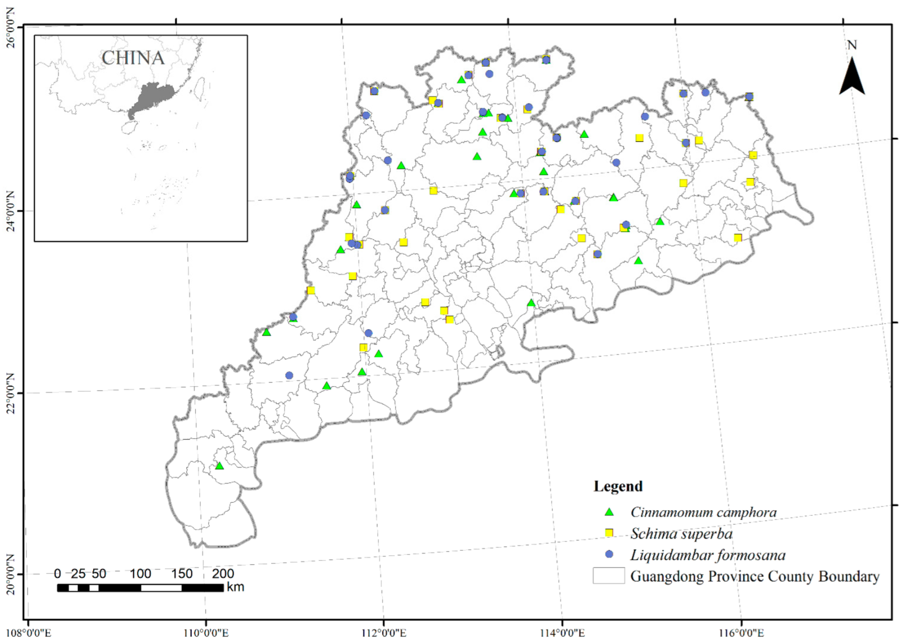
2.1. Study Area

This study was conducted in Guangdong Province (109°45′–117°20′ E, 20°09′–25°31′ N), which covers an area of 179,700 km2. The terrain of this area is high in the north and low in the south, dominated by low mountains and hills. The area belongs to the East Asian monsoon region which is rich in sun exposure, heat, and water resources. The main vegetation types are mid-subtropical evergreen broad-leaved forests, southern subtropical evergreen broad-leaved forests, and tropical monsoon forests. C. camphora, S. superba, and L. formosana are the main native tree species and the main tree species used for carbon sink afforestation, which together account for more than 50% of the total carbon sink afforestation efforts in Guangdong [40]. Samples were distributed evenly across Guangdong according to the tree species ratio and diameter grade ratio that originated from the Chinese National Forest Inventory in 2012, as shown in Figure 1.

2.2. Diameter Data

Data from 120 tree samples were collected composed of C. camphora, S. superba, and L. formosana. Tree samples were gotten by typical sampling to collect information on different growth conditions. Each diameter grade had more than 5 samples with different growth conditions (tree height). A diameter series obtained from stem analysis formed the base data for modeling. The DBHs of sample trees were measured before felling. After felling, 120 sample trees were selected for stem analysis. First, discs were taken at positions of the stump (0.3 m) and breast height (1.3 m). Then, a disc was taken every 2 m starting from a distance above 1.3 m. Finally, discs were taken at 1-m intervals when the end of the tree was more than 1 m but less than 2 m. The diameters of the annual ring at stump (0.3 m, No.0 disc) and breast height (1.3 m, No.1 disc) were averages, measured from east to west and north to south through the LINTAB annual ring analysis system [23], which composed diameter series of individual trees. In the field measurement, trees with diameters < 5 cm were not chosen. To simulate field measurement, data with diameter < 5 cm were excluded from the diameter series. As such, d0 represents the minimum diameter (as initial diameter) and is > 5 cm. The initial age is the time at which the diameter grows from 0 to d0. Time intervals are corresponding tree age intervals between the minimum diameter and other diameters. Finally, the diameter series at stump and breast height were obtained. Table 1 lists the summary statistics of sampled tree age and diameter inside bark (DIB) per species at different heights.
Individual tree diameter series do not contain information about intra-specific variability. Considering dynamic associations among the same species, panel data (a data structure commonly used in econometrics) was used. Panel data is multi-dimensional data containing observations about different cross sections across time. Each value in the panel data is denoted as yit, where i represents the ith individual and t represents the tth observation period [41]. If the individuals in the sample were identical in each period, the sample is called a “balanced panel”, otherwise it is called an “unbalanced panel” [42]. Modeling panel data can not only control the time-invariant and unobservable heterogeneous factors, but also the time-varying and unobservable homogeneous factors, which makes parameter estimation more reliable [41]. Compared with cross-sectional data or time series, panel data is more conducive for studying dynamic changes within data sets [43,44].
In this paper, the diameter data of an individual tree presents a typical time series. Panel data consists of individual tree diameter series of the same tree species. Panel data is unbalanced because different individual trees have different series lengths. Due to a large number of rows in the panel data, some data are not shown in Table 2.

2.3. Methods

2.3.1. Base Growth Equations

Lundqvist–Korf, Richards, Monomolecular, and Logistic equations are widely used in tree growth modeling [45,46,47]. These four equations were selected as the base equation for estimating tree age. The Richards equation was used as an example and was calculated according to Equation (1):
d t = a ( 1 e b t ) c
where dt is the diameter obtained by measuring the annual ring width, t is the age i.e., the number of annual rings, and a, b, c are model parameters. Parameter a is the limit value parameter of the growth of the tree diameter. Parameter b is related to the tree growth rate in Richards or Monomolecular equations and reflects the intrinsic growth rate in the Logistic equation. Moreover, parameter b is related to the intrinsic growth rate and attenuation power exponent in the Korf equation. Parameter c is a shape parameter, which is related to the power exponent of the assimilation in the Richards equation and related to the attenuation factor in plant growth in the Korf equation [48,49].

2.3.2. Constraint Growth Equations

Exploratory research showed that fitting effects using base equations were unstable. Therefore, a constraint was used that ensured that the growth curve passed through the point (0, d0), which made models more stable.
Bailey and Clutter [50] derived the base-age invariant model using an algebraic difference approach which allowed one parameter to be subject-specific. This model produced anamorphic site curves of a New Zealand pine plantation. On this basis, Cieszewski and Bailey [51] proposed a generalized algebraic difference approach that considered more than one parameter as subject-specific parameters. This model produced polymorphic curves with multiple asymptotes. The present research adopted an algebraic approach inspired by this generalized algebraic difference approach. The calculation details are summarized in the following:
Replacing the variable t in the base model with unknown initial age plus time interval, the new growth function was obtained as shown in Equation (2):
d = a [ 1 e b ( t + a g e 0 ) ] c
where t′ is the time interval and age0 is the initial age. The meanings of other parameters are the same as those used in Equation (1). In fact, Equation (2) is another special solution to the exponential growth equation for t′ = 0 and d = d0 [45]. age0 from Equation (2) was assumed as a specific parameter and solved for age0:
a g e 0 = ln ( 1 ( d a ) 1 c ) b t
By substituting initial values (0, d0) into t′ and d, the algebraic solution of age0 was obtained. Substituting this assumption into Equation (2), the constraint growth equation based on the Richards equation was obtained, as shown in Equations (4) and (5):
d = a [ 1 e b · ( t + a g e 0 ) ] c
where
a g e 0 = ln ( 1 ( d 0 a ) 1 c ) b
After setting age0 as a specific parameter, the other three base growth equations could also be derived with constraints similarly (Table 3).

2.3.3. First-Order Difference Method

The first-order difference method is always suitable for the case where the original model has a high degree of first-order autocorrelation [52]. Using the first-order difference method, the difference constraint growth equation was developed as shown in the following:
Δ d t = a [ 1 e b ( t + 1 + a g e 0 ) ] c a [ 1 e b ( t + a g e 0 ) ] c
where
Δ d t = d t + 1 d t ,   a g e 0 = ln ( 1 ( d 0 a ) 1 c ) b
In Equation (6), t′ is the time interval, age0 is the initial age, Δdt is the diameter increment in the time interval t′, and other parameters have the same meaning as above. The difference constraint equation is the increment equation. Similarly, the difference forms with constraints of other base equations are shown in Table 3.

2.3.4. Diameter Increment Equation with Parameter A-Classification

A diameter increment equation with parameter a-classification was proposed to improve suitability. In this process, the fitting data was the panel data composed of the diameter series of the same species and heights. Parameter a was allowed to vary and parameters b and c were held as a single value for the same fitting data, as b and c were related to the inherent properties of tree species and a was related to the site. In the model without parameter classification, parameter a was the most unstable. Further experiments showed that among the models with one parameter classification and the other two parameters maintaining a single value, the model with parameter a-classification had the best goodness of fit. a-classification constructed from dummy variables improved the applicability of the model [53]. Taking Richards equation as the base equation, the steps to establish the equation were as follows:
Step 1: Using the dummy variable method, dummy variables were generated to indicate tree-specific parameters. For difference constraint Equations (6) and (7), the dummy variable models were given as:
Δ d i t = a { [ 1 e b ( t + 1 + a g e i 0 ) ] c [ 1 e b ( t + a g e i 0 ) ] c }
where
a g e i 0 = ln ( 1 ( d i 0 a ) 1 c ) b , a = a 1 + i = 2 m S i × a i
In Equations (8) and (9), Δdit is the diameter increment in time interval t′ for ith sample tree, m is the number of sample trees, t′ is the time interval, agei0, and di0 are initial age and initial diameter for the ith sample tree, respectively, Si is the dummy variable with value of 1 for the ith sample tree and 0 otherwise (except S1 is a constant with value of 1), ai is the tree-specific parameter, and i is ranged from 1 to m. The meanings of other parameters are the same as above.
Step 2: The appropriate number of classes was selected based on sample size, and five classes were chosen. Estimated values of parameter a obtained by Step 1 were clustered using one-dimensional K-means clustering to obtain the class each sample tree belonged to [54,55].
Step 3: Using the dummy variable method, dummy variables were generated to indicate class-specific parameters. The dummy variable model can be specified as
Δ d i t = a { [ 1 e b ( t + 1 + a g e i 0 ) ] c [ 1 e b ( t + a g e i 0 ) ] c }
where
a g e i 0 = ln ( 1 ( d i 0 a ) 1 c ) b , a = a 1 + j = 2 g L j × a j
In Equations (10) and (11), g is the number of classes, Lj is the dummy variable with value of 1 for the jth class in which ith sample tree belongs to and 0 otherwise (except L1 is a constant with value of 1), aj is the class-specific parameter, and j is ranged from 1 to g. The meanings of other variables and parameters are the same as above.
Step 4: The estimated initial age of each sample tree was calculated using the estimated value of parameters in Step 3, as shown in Equation (12):
a g e ^ i 0 = ln ( 1 ( d i 0 a ^ c l a s s ) 1 c ^ ) b ^
where a g e ^ i 0 is the estimated initial age for ith sample tree, a ^ c l a s s is the estimated value of a in the class that ith sample tree belongs to, and b ^ , c ^ are the parameter estimates of b, c in Equation (10), respectively.
Step 5: The estimated age in each period was obtained by adding the estimated initial age to the time interval, as ( a g e ^ i 0 + t ).
Similarly, the same steps were used for other growth equations.

2.3.5. Quality of Fit and Verification

The fitting models were evaluated using the adjusted coefficient of determination (R2adj), the standard estimated error (SEE), and the mean prediction error (MPE), using Equations (13)–(15).
R a d j 2 = 1 i = 1 n ( y i y ^ i ) 2 / ( n p 1 ) i = 1 n ( y i y ¯ ) 2 / ( n 1 )
S E E = i = 1 n ( y ^ i y i ) 2 / ( n p )
M P E = t α × ( S E E / y ¯ ) / n × 100
where yi is the diameter increment for ith sample tree, y ^ i is the estimated value of yi, y ¯ is the average value of yi, n is the number of samples, p is the number of parameters in the equation, and t α is the t-value when the confidence level is 1-a.
The model was validated by comparing estimated ages with the real tree ages obtained from stem analysis. The accuracy of the validation was calculated using the mean error (ME), the mean absolute error (MAE), and the root mean square error (RMSE), as shown in Equations (16)–(18).
M E = 1 n × i = 1 n ( a g e i a g e ^ i )
M A E = 1 n × i = 1 n | a g e i a g e ^ i |
R M S E = 1 n × i = 1 n ( a g e i a g e ^ i ) 2
where agei is the true age for the ith sample tree, a g e ^ i is the estimated value of agei, and n is the number of samples.

3. Results

3.1. Selection of Base Growth Equation Based on Individual Tree Diameter Data

To select the most suitable base growth equation and analyze autocorrelated residuals, known age and diameter series were used to fit different base equations (as shown in Table 3).

3.1.1. Fitting Results from Base Growth Equation

Table 4 shows the fitting results. At the individual tree scale, the fitting results and parameters robustness of different equations differed. From the perspective of fitting results, the Richards equation and Logistic equation converged more readily than the Korf equation and Monomolecular equation. In terms of distributions of parameter estimates, the estimated parameters of the Richards equation and Logistic equation were more concentrated than the Korf equation and Monomolecular equation. The biological meaning of parameter a in the growth equations is the asymptote. The maximum DIB (see Table 1), derived from field measurement, was close to the estimated parameter a in the Richards equation. Therefore, the Richards equation was chosen to develop the diameter increment equation.

3.1.2. Autocorrelation Test and Treatment

Based on fitting the diameter series results at breast height, the residuals were calculated and the presence of autocorrelation was detected by the Durbin–Watson (DW) test. At a 5% significance level, if the DW statistic is in the interval [0, 1.39], the series has a positive autocorrelation, if it is in the interval [2.61, 4], the series has a negative autocorrelation with reference to the DW test table [52,56]. The results showed that approximately 48% of the DW statistics of the individual tree diameter series regression fell within the interval [0,1.39] except for certain non-convergent results, for which it can be assumed that the diameter series had autocorrelation. Table 5 shows the results of the DW test. The orders of autocorrelation can be roughly determined by observing the autocorrelation figure and partial correlation figure. In the test results, the first-order and second-order autocorrelation in the residuals accounted for about 32% and 20% of the total samples. About 1% had third-order autocorrelation and above. About 21% did not have autocorrelation and about 26% of samples could not be accurately judged. The difference method can handle autocorrelation, so the difference constraint growth equation was developed (Equations (6)–(7)) and was also called increment equations.

3.2. Increment Equation with Parameter Classification Based on Panel data

According to the fitting results based on the individual tree diameter series shown in Table 4, the estimated value of parameters fluctuated greatly on the individual tree scale. For example, when fitting the diameter series at stump height for C. camphora using the Richards equation, the estimated parameter c ranged from 1.03 to 14.2, indicating poor stability. This was because the intra-specific correlation was ignored. The panel data was composed of all the individual tree diameter series in the same species; therefore, the intra-specific correlations could be fully considered. To model the panel data, diameter increment equations with parameter a-classification were developed.

3.2.1. Fitting Evaluation

Fitting effects based on the panel data were better than fitting the diameter series (Table 6). The range of the SEEs was from 0.23 to 0.33, and the MPEs were below 2.5% for different tree species and different heights, but the R2s were not high, and ranged mainly from 0.59 to 0.7. All estimated values of parameters were statistically significant because p-values were less than 0.01. Table 6 shows t-values of parameter estimates. T-values in Table 6 were larger than 2.58 (the t-stat value at 1% significance level on sample degrees of freedom). Overall, the fitting result was relatively good. The estimated parameter a gradually increased from class 1 to 5, which means that trees in different classes had different growth environments. The estimated parameter b was distributed mainly around 0.02, and the estimated value of parameter c was around 1.
The estimated values of each parameter were substituted into Equation (12) to estimate the initial age. This approach achieved good precision of tree age estimation (Table 7). Except for C. camphora at stump height and S. superba at breast height, MEs were all in the interval [−1,1], RMSEs were less than 3 years, and MAEs were less than 2 years. Estimated tree ages for C. camphora at stump and S. superba at breast height were underestimated. Error standard deviations for L. formosana at the two heights were 2.59 and 2.44, respectively, which were slightly larger than for the other two tree species.
Errors were mainly distributed in the interval [−5, 5] except for a few outliers (Figure 2). Median errors for C. camphora and S. superba exceeded 0, especially for C. camphora at stump height and S. superba at breast height, indicating that the approach slightly underestimated their ages. The estimation error for L. formosa was more evenly distributed around 0, while the outliers caused large error standard deviations. In general, the error of individual tree age estimates using the approach was small and the estimation accuracy of different tree species differed. Through error check-up, a phenomenon is that the error size was not directly related to diameters, but was related to the diameter growth rate at the young tree stage (diameter < 5 cm). If the diameter growth rate at the young tree stage is small, their estimation errors are relatively large. This phenomenon is obvious for C. camphora at stump height and S. superba at breast height.

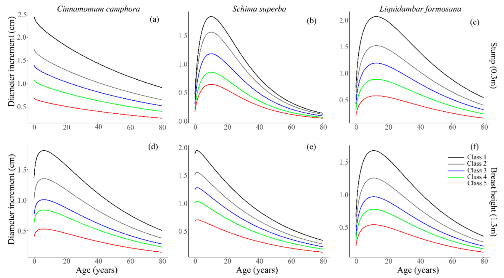
3.2.2. Comparison of Fitting Diameter Panel Data at Different Heights

From the perspective of model fitting (Table 6), compared with the panel data at stump height, R2adjs for modeling based on the panel data at breast height increased by 0.02, 0.02, and 0.06, SEEs decreased by 0.06, 0.03, and 0.05, and MPEs decreased by 0.07%, −0.02%, and 0.22% for the three species, respectively. As a result, the fitting effect of the panel data was better at breast height. For C. camphora and L. formosana, the estimated value of parameter a of the panel data at breast height was smaller than the estimated value of the panel data at stump height, while this was the opposite for S. superba. The estimated values of parameter b and parameter c had no obvious difference between the different heights.
From the perspective of tree age estimation (Table 7), compared with the panel data at stump height, MAEs for modeling based on the panel data at breast height decreased by 1.69 and 0.18 years and RMSEs had decreased by 1.85 and 0.12 years for C. camphora and L. formosana, respectively. However, for S. superba, MAE for the panel data at breast height increased by 0.79 years, and RMSE increased by 0.73 years. Among the three tree species, the error standard deviation based on the panel data at breast height was lower. For C. camphora, the error estimated based on the panel data at breast height was closer to 0 and the interquartile range of the error was smaller, while this was the opposite for S. superba. For L. formosana, the difference between the two heights was not apparent (Figure 2). Overall, based on the panel data at breast height, the average MAE for the three species was 1.97 years and the average RMSE was 2.55 years. Based on the panel data at stump height, the average MAE for the three species was 2.33 years and the average RMSE was 2.97 years. Therefore, the estimated effect based on the panel data at breast height was better for C. camphora and L. formosana, and the estimated effect based on the panel data at stump height was better for S. superba.

4. Discussion

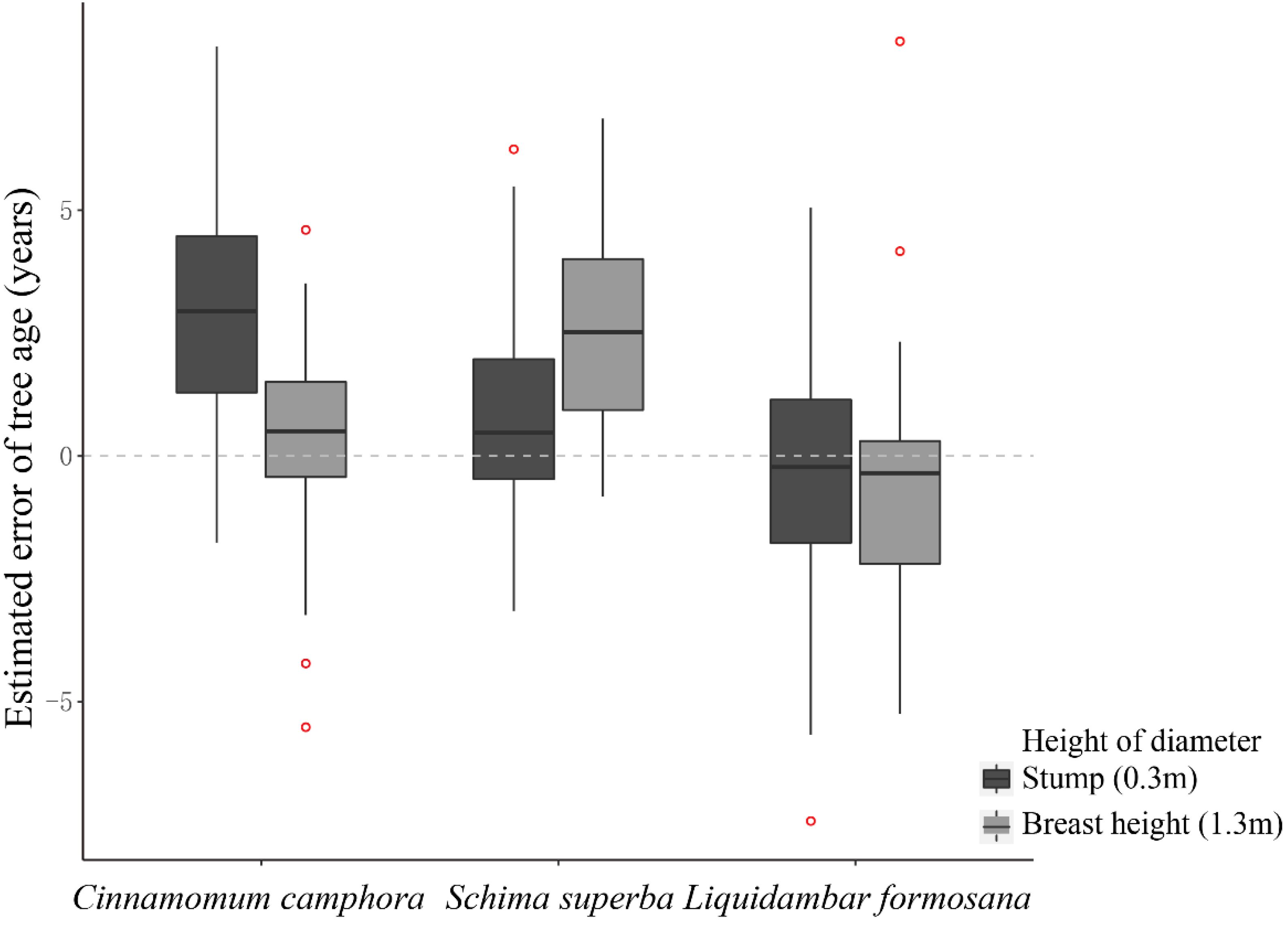
4.1. Estimation and Applicability

Based on the modeling results of the base growth equation, the Richards equation was chosen as the optimal base equation for individual trees. The parameter classification method was used to improve the suitability of the equation, because sample plots were widely distributed, and their environments were different. Dummy variables were generated to indicate class-specific parameters. Parameter a was taken as the class-specific parameter. Then, diameter increment equations with parameter a-classification were used to obtain several lifetime growth curves. A range of tree ages was obtained using the approach for a given diameter series and the first flaw was eliminated. The diameter growth increment curve clusters for three tree species at two heights are drawn in Figure 3. Diameter increment curve clusters reflect several growth conditions. Their shapes were unimodal and the maximum increment value increased with growth potentials except for C. camphora at a stump height (0.3 m). However, the ages at which the diameter increment reached the maximum value on different growth curves were identical, which was caused by the same values of parameters b and c in different classes. When the estimated value of parameter c was close to 1, there was either no extreme point or the extreme point appeared very early in the diameter increment curve. For example, the diameter increment for C. camphora at stump height decreased monotonously with age, and the extreme point of the diameter increment curve for S. superba at breast height already appeared when the tree was very young. The age at which diameter increment reached the maximum value for S. superba was less than that for L. formosana.
The estimated age obtained by this approach was validated using age data independently obtained from stem analysis. Tree age estimation achieved high precision. RMSEs of ages at breast height for C. camphora and L. formosana were 1.85 years and 0.12 years lower than at stump height, while the RMSE of ages at breast height for S. superba was 0.73 years higher (Table 7). However, tree ages at breast height ignore the time for the tree to grow to breast height [7,57]. Ages at stump height were closer to the real tree age, but ages at breast height obtained better estimated results. Therefore, the second flaw that existed in previous age estimation methods was also eliminated.
In previous studies, Kalliovirta and Tokola [32] used tree height and maximum crown width to predict tree ages and achieved RMSEs of 9.2% to 12.8% of the average age, while tree height and crown width were difficult to measure. Silva et al. [3] established a growth model of tree age, tree height, DBH, and other tree measuring factors to estimate tree age with an RMSE of around 9 years. Pan et al. [26] estimated tree age based on spectrum analysis and obtained a MAE of 2 years, however, this approach needs to be tested in more tree species but has great development potential. Age estimation using the proposed approach provides good precision. MAEs of age at breast height for C. camphora, S. superba, and L. formosana were 1.55, 2.59, and 1.76 years, respectively. RMSEs were 2.04, 3.15, and 2.47 years, accounting for 6.07%, 11.08%, and 7.19% of the average age of each species, respectively.
The approach was proposed for tree diameter data measured in forest inventory. The diameter series obtained from stem analysis in this paper was to simulate diameter data measured in the field, both of which were time series. The stem analysis can also obtain real tree ages and then use the real ages to validate this method. In practical application, modeling data are from diameter data measured in the field. To overcome autocorrelation, we consider the difference method and developed a different form of the diameter equation. Hence, the diameter increment data and time interval data were needed to estimate the tree age. The diameter increment data can be obtained by subtracting the diameter measured earlier from the diameter measured later. Time intervals are the time from the initial diameter measurement to each measurement.
Hence, the proposed approach can estimate tree age using diameter data measured in the field rather than increment core (or stem disc) data. Based on diameter data measured in the field, diameter increment (Δdit) data are calculated and time interval (t′) data are obtained. The diameter measured initially (di0) is also recorded. These data are modeled with Δdit as the dependent variable and t′, di0 as the independent variable according to steps in Section 2.3.4. The estimated initial age is calculated using the estimated value of parameters according to Equation (11).
This approach can also be applied to new trees. If new trees belong to the tree species that are involved in modeling and come from the same study region, diameter data measured in at least two periods are required, and the steps to apply the approach to new trees are as follows: firstly, choosing a value of class i for parameter a (estimated by Equation (10) and (11)) and substituting the two field-measured diameter data into Equation 19, respectively, two estimated ages such as agei1 and agei2 of the two measurements are obtained. This step needs to be performed for each class of parameter a. The constant g is the number of classes and g groups of estimated ages (agei1 and agei2, i = 1,2, …, g) for a tree are obtained through this step. Then, the difference value (D-value) between the two ages for each class of parameter a needs to be recorded (g classes of parameter a get g differences value: D1, D2, …, Dm). Comparing the D-value with the actual measurement time interval, the class of parameter a with the smallest change between the D-values and the measurement time interval was selected as the appropriate class of this new tree.
a g e ^ M T = ln ( 1 ( d M T a ^ c l a s s ) 1 c ^ s p e c i e s ) b ^ s p e c i e s
where a g e ^ M T is the estimated age at measurement time, dMT is the measured diameter, a ^ c l a s s is the estimated value of a in classes, and b ^ s p e c i e s , c ^ s p e c i e s are the parameter estimates of b, c of the tree species in Equation (10), respectively. But if new trees don’t belong to tree species involved in the modeling or come from other study regions, they cannot be calculated using the steps above, but instead need sufficient samples to repeat the modeling process in 2.3.4.
The applicability of the model is discussed from the perspectives of the usage scenario, sample collection, and validation. The first key point of method applicability is the usage scenario of the approach. This approach is proposed for diameter data measured in forest inventory and can estimate tree age using diameter data measured in the field. Stem discs are important for validating this approach rather than modeling.
The second key point of method applicability is the collection of model-building samples. The sample size and sampling range have impacts on modeling. The sample size for modeling should fulfill the statistical requirements and should be much larger than the number of parameters. The sampling range refers not only to the range where the sample data were collected, but also to the range of different growth conditions. These factors determine the appropriate number of classes. Model-building samples need to contain comprehensive growth information, so the established model can be applied to samples of various growth environments. It is worth mentioning that the number of samples for each species is not the best sample size to develop this equation. Model accuracy may improve further if the sample size is increased.
The third key point of method applicability is validation. The estimation effect needs to be evaluated in the application. When this method is applied to new trees, whether the accuracy of tree age estimation needs to be re-evaluated mainly depends on tree species and the sampling region, because different estimated values of parameters and different estimated effects may be obtained. This approach was applied to subtropical tree species with high accuracy. The accuracy of the approach applied to tree species in other climate regions needs to be evaluated.

4.2. Equation Structure Analysis

To improve the estimation stability, an algebraic structure similar to the generalized algebraic difference approach was used [50,58]. The difference is that no new variables were introduced into the growth function (Equation (4)). A constraint on the growth equations was added by making the growth curve pass through the initial point (0, d0). Furthermore, another constraint was also considered that the growth curve passed through the point (t′, dt)median corresponding to the median of the diameter sequence. Under this constraint, the MAE of the estimated age at breast height was less than 4.5 years, and the MAE at stump height was less than 3 years. Compared with the equations with the first constraint (the initial point), there was not much difference in estimation accuracy for C. camphora and S. superba, but the estimated error was larger for L. formosana. Therefore, the estimation effect of taking the initial point (0, d0) as the initial condition was better. The selection of the initial value impacted tree age estimation, but it tended to be stable.
To further understand the influence of class-specific parameters, parameter b was taken as the class-specific parameter and the two other parameters maintained a single value in the same species and heights. Table 8 shows the estimated error of tree age from the diameter increment equations with parameter b-classification. The estimation result was slightly worse compared with a-classification. For example, when fitting the panel data at stump height for C. camphora, the estimated a and b were not significant, and age estimation obtained a large error for L. formosana at stump height. The result showed that b-classification was not sufficiently stable to estimate different tree species. The diameter increment equation with parameter c-classification was also not ideal for estimating tree age.
Parameters b and c had lower numeric values and were related to the inherent properties of the tree species. Hence, parameter a was taken as a class-specific parameter while constraining parameters b and c to be the same for the same species and heights. The variability between different sites and intra-specific variability was considered by this approach.

4.3. Autocorrelation and Processing

Autocorrelation existed in the residuals of age estimation. In previous research, the first-order autoregressive error structure (AR1) was used to deal with such autocorrelation in forestry. Li and Weiskittel [38] improved the traditional AR1 and opted to use the CAR1 correlation structure, which was a continuous version of AR1. In addition, the mixed-effect model was also a good way to deal with autocorrelation [38,59]. In this study, by test statistics (involving the DW statistic and the Breusch–Godfrey statistic) and observation of partial correlation figures, autocorrelation was found to exist in more than 50% of sample trees, which was consistent with the above-mentioned literatures’ judgment regarding autocorrelation. Considering the applicability of the model and previous scholars’ research experiences [34,38,59,60], for this paper, the first-order difference method was adopted. This approach enabled efficient processing of autocorrelation while it was not sufficiently strict because different autocorrelation orders appeared in the residuals. This imposed higher requirements for the form of the difference equation.
In the past, few scholars have focused on the orders of autocorrelation in forestry research. The DW test can only detect the presence of first-order autocorrelation [61]. The Breusch–Godfrey statistic and partial correlation figures have been used to detect high-order autocorrelation. In this study, first-order and second-order autocorrelation were common in the tree diameter series, accounting for over 52% of the total samples. There were residuals that cannot be accurately judged because either the diameter series size was too small or the partial correlation figure lacked regularity. Autocorrelation violates the Gauss–Markov condition in the base assumptions of the regression model. Although the parameters passed the test, the variance of the parameter estimation has not reached the minimum, which means that the best unbiased estimator has not yet been identified.

5. Conclusions

In this paper, a diameter increment equation with parameter a-classification was developed for estimating individual tree age. Panel data contained intra-species information, which was helpful for modeling. The parameter classification method improved the suitability of the equation. Validation was done using the real tree age obtained from stem analysis for three subtropical tree species. MAEs of the estimated tree ages for the three tree species were less than 3.5 years and RMSEs were less than 4 years. The estimated result for L. formosana was the most stable, and its MAE was less than 2 years. The estimated results for C. camphora and L. formosana based on the panel data at breast height were better than at stump height, while this was the opposite for S. superba. Furthermore, first-order and second-order autocorrelations were more common in the tree diameter series, whilst higher-order autocorrelation was rare. Overall, the developed approach improves the accuracy and parameter stability for estimating individual tree age and provides a feasible way to obtain tree age in field measurement.

Author Contributions

Methodology, H.L.; formal analysis, Y.Z.; resources, H.L.; data curation, H.L. and J.H.; writing—original draft preparation, Y.Z.; writing—review and editing, H.L., X.Z., Y.L., Y.Z. and X.L.; visualization, Y.Z.; supervision, H.L., Y.L. and X.Z. All authors have read and agreed to the published version of the manuscript.

Funding

The research was supported by the Central Public-Interest Scientific Institution Basal Research Fund (grant number CAFYBB2018ZB006), the National Natural Science Foundations of China (grant number 31770676, 31872704), the Guangdong Forestry Science and Technology Special Project (2015-02), and the Guangdong Forestry Science and Technology Innovation Construction Project (2016CXPT03).

Data Availability Statement

Not applicable.

Conflicts of Interest

The authors declare no conflict of interest.

References

  1. Crecente-Campo, F.; Dieguez-Aranda, U.; Rodriguez-Soalleiro, R. Resource communication. Individual-tree growth model for radiata pine plantations in northwestern Spain. For. Syst. 2012, 21, 538–542. [Google Scholar] [CrossRef]
  2. Garet, J.; Raulier, F.; Pothier, D.; Cumming, S.G. Forest age class structures as indicators of sustainability in boreal forest: Are we measuring them correctly? Ecol. Indic. 2012, 23, 202–210. [Google Scholar] [CrossRef]
  3. Silva, L.B.; Teixeira, A.; Alves, M.; Elias, R.B.; Silva, L. Tree age determination in the widespread woody plant invader Pittosporum undulatum. For. Ecol. Manag. 2017, 400, 457–467. [Google Scholar] [CrossRef]
  4. Hu, M.; Lehtonen, A.; Minunno, F.; Mäkelä, A. Age effect on tree structure and biomass allocation in Scots pine (Pinus sylvestris L.) and Norway spruce (Picea abies [L.] Karst.). Ann. For. Sci. 2020, 77, 90. [Google Scholar] [CrossRef]
  5. Hipler, S.M.; Spiecker, H.; Wu, S.R. Dynamic Top Height Growth Models for Eight Native Tree Species in a Cool-Temperate Region in Northeast China. Forests 2021, 12, 965. [Google Scholar] [CrossRef]
  6. Reyes-Palomeque, G.; Dupuy, J.M.; Portillo-Quintero, C.A.; Andrade, J.L.; Tun-Dzul, F.J.; Hernández-Stefanoni, J.L. Mapping forest age and characterizing vegetation structure and species composition in tropical dry forests. Ecol. Indic. 2021, 120, 106955. [Google Scholar] [CrossRef]
  7. Wong, C.M.; Lertzman, K.P. Errors in estimating tree age: Implications for studies of stand dynamics. Can. J. For. Res. 2001, 31, 1262–1271. [Google Scholar] [CrossRef]
  8. Nath, C.D.; Boura, A.; De Franceschi, D.; Pélissier, R. Assessing the utility of direct and indirect methods for estimating tropical tree age in the Western Ghats, India. Trees-Struct. Funct. 2012, 26, 1017–1029. [Google Scholar] [CrossRef]
  9. Fontes, L.; Tome, M.; Coelho, M.B.; Wright, H.; Luis, J.S.; Savill, P. Modelling dominant height growth of Douglas-fir (Pseudotsuga menziesii (Mirb.) Franco) in Portugal. Forestry 2003, 76, 509–523. [Google Scholar] [CrossRef] [Green Version]
  10. Forrester, D.I.; Tachauer, I.H.H.; Annighoefer, P.; Barbeito, I.; Pretzsch, H.; Ruiz-Peinado, R.; Stark, H.; Vacchiano, G.; Zlatanov, T.; Chakraborty, T.; et al. Generalized biomass and leaf area allometric equations for European tree species incorporating stand structure, tree age and climate. For. Ecol. Manag. 2017, 396, 160–175. [Google Scholar] [CrossRef]
  11. Lei, X.D.; Fu, L.Y.; Li, H.; Li, Y.T.; Tang, S.Z. Methodology and Applications of Site Quality Assessment Based on Potential Mean Annual Increment. Sci. Silvae Sin. 2018, 54, 116–126. (In Chinese) [Google Scholar] [CrossRef]
  12. Zhang, H.R.; Lei, X.D.; Zhang, C.Y.; Zhao, X.H.; Hu, X.F. Research on theory and technology of forest quality evaluation and precision improvement. J. Beijing For. Univ. 2019, 41, 1–18. (In Chinese) [Google Scholar] [CrossRef]
  13. Duerr, W.A.; Gevorkiantz, S.R. Growth prediction and site determination in uneven-aged timber stands. J. Agric. Res. 1938, 56, 81–98. [Google Scholar]
  14. Ek, A.R. A comparison of some estimators in forest sampling. For. Sci. 1971, 17, 2–13. [Google Scholar]
  15. Carmean, W.H.; Lenthall, D.J. Height-growth and site-index curves for jack pine in north central ontario. Can. J. For. Res.-Rev. Can. Rech. For. 1989, 19, 215–224. [Google Scholar] [CrossRef]
  16. Cieszewski, C.J.; Zasada, M.; Borders, B.E.; Lowe, R.C.; Zawadzki, J.; Clutter, M.L.; Daniels, R.F. Spatially explicit sustainability analysis of long-term fiber supply in Georgia, USA. For. Ecol. Manag. 2004, 187, 345–359. [Google Scholar] [CrossRef]
  17. Stokes, M.A.; Smiley, T.L. An Introduction to Tree-Ring Dating; University of Chicago Press: Chicago, IL, USA, 1968. [Google Scholar]
  18. Norton, D.A.; Palmer, J.G.; Ogden, J. Dendroecological studies in New Zealand 1. An evaluation of tree age estimates based on increment cores. N. Z. J. Bot. 1987, 25, 373–383. [Google Scholar] [CrossRef]
  19. Agren, J.; Zackrisson, O. Age and size structure of Pinus sylvestris populations on mires in central and northern Sweden. J. Ecol. 1990, 78, 1049–1062. [Google Scholar] [CrossRef]
  20. Lusk, C.; Ogden, J. Age structure and dynamics of a podocarp broadleaf forest in Tongariro National Park, New Zealand. J. Ecol. 1992, 80, 379–393. [Google Scholar] [CrossRef]
  21. Szeicz, J.M.; Macdonald, G.M. Recent white spruce dynamics at the subarctic alpine treeline of north-western Canada. J. Ecol. 1995, 83, 873–885. [Google Scholar] [CrossRef]
  22. Rozas, V. Tree age estimates in Fagus sylvatica and Quercus robur: Testing previous and improved methods. Plant Ecol. 2003, 167, 193–212. [Google Scholar] [CrossRef]
  23. Oh, J.-A.; Seo, J.-W.; Byung-Ro, K. Verifying the Possibility of Investigating Tree Ages Using Resistograph. J. Korean Wood Sci. Technol. 2019, 47, 90–100. [Google Scholar] [CrossRef]
  24. Wang, S.Y.; Chiu, C.M.; Lin, C.J. Application of the drilling resistance method for annual ring characteristics: Evaluation of Taiwania (Taiwania cryptomeribides) trees grown with different thinning and pruning treatments. J. Wood Sci. 2003, 49, 116–124. [Google Scholar] [CrossRef]
  25. Orozco-Aguilar, L.; Nitschke, C.R.; Livesley, S.J.; Brack, C.; Johnstone, D. Testing the accuracy of resistance drilling to assess tree growth rate and the relationship to past climatic conditions. Urban For. Urban Green. 2018, 36, 1–12. [Google Scholar] [CrossRef]
  26. Pan, H.; Lu, J.; Guo, X.Z.; Tang, S.Z.; Gao, R.D.; Xu, J.J. Tree age estimation algorithm based on spectrum analysis by Resistograph. For. Res. 2021, 34, 19–25. (In Chinese) [Google Scholar] [CrossRef]
  27. Rinn, F.; Schweingruber, F.H.; Schar, E. RESISTOGRAPH and X-ray density charts of wood comparative evaluation of drill resistance profiles and X-ray density charts of different wood species. Holzforschung 1996, 50, 303–311. [Google Scholar] [CrossRef]
  28. Jahan, M.S.; Mun, S.P. Effect of tree age on the cellulose structure of Nalita wood (Trema orientalis). Wood Sci. Technol. 2005, 39, 367–373. [Google Scholar] [CrossRef]
  29. Poussart, P.M.; Myneni, S.C.B.; Lanzirotti, A. Tropical dendrochemistry: A novel approach to estimate age and growth from ringless trees. Geophys. Res. Lett. 2006, 33. [Google Scholar] [CrossRef] [Green Version]
  30. Wu, W.N.; Wan, T. Progress of dating methods of tree age. J. Green Sci. Technol. 2013, 7, 152–155. (In Chinese) [Google Scholar]
  31. Baker, P.J. Tree age estimation for the tropics: A test from the southern appalachians. Ecol. Appl. 2003, 13, 1718–1732. [Google Scholar] [CrossRef]
  32. Kalliovirta, J.; Tokola, T. Functions for estimating stem diameter and tree age using tree height, crown width and existing stand database information. Silva Fenn. 2005, 39, 227–248. [Google Scholar] [CrossRef] [Green Version]
  33. Hu, Y.Y.; Kang, X.G.; Zhao, J.H. Variable relationship between tree age and diameter at breast height for natural forests in Changbai Mountains. J. Northeast. For. Univ. 2009, 37, 38–42. (In Chinese) [Google Scholar]
  34. Koirala, A.; Montes, C.R.; Bullock, B.P.; Wagle, B.H. Developing taper equations for planted teak (Tectona grandis L.f.) trees of central lowland Nepal. Trees For. People 2021, 5, 100103. [Google Scholar] [CrossRef]
  35. Wang, M.; Borders, B.E.; Zhao, D. An empirical comparison of two subject-specific approaches to dominant heights modeling: The dummy variable method and the mixed model method. For. Ecol. Manag. 2008, 255, 2659–2669. [Google Scholar] [CrossRef]
  36. Sharma, R.P.; Zdeněk, V.; Stanislav, V.; Václav, J.; Miloš, K. Modelling individual tree diameter growth for Norway spruce in the Czech Republic using a generalized algebraic difference approach. J. For. Sci. 2017, 63, 227–238. [Google Scholar] [CrossRef] [Green Version]
  37. Davidian, M.; Giltinan, D.M. Nonlinear models for repeated measurement data: An overview and update. J. Agric. Biol. Environ. Stat. 2003, 8, 387–419. [Google Scholar] [CrossRef]
  38. Li, R.; Weiskittel, A.R. Comparison of model forms for estimating stem taper and volume in the primary conifer species of the North American Acadian Region. Ann. For. Sci. 2010, 67, 302. [Google Scholar] [CrossRef] [Green Version]
  39. Clark, J.S. Coastal forest tree populations in a changing environment, southeastern Long-Island, New-York. Ecol. Monogr. 1986, 56, 259–277. [Google Scholar] [CrossRef]
  40. Xue, C.Q.; Xu, Q.H.; Lin, L.P.; He, X.; Luo, Y.; Zhao, H.; Cao, L.; Lei, Y.C. Biomass models with breast height diameter and age for main nativetree species in Guangdong Province. Sci. Silvae Sin. 2019, 55, 97–108. (In Chinese) [Google Scholar] [CrossRef]
  41. Bai, Z.L. Econometric Analysis of Panel Data; Nankai University Press: Tianjin, China, 2008. (In Chinese) [Google Scholar]
  42. Chen, Q. Advanced Econometrics and Stata Application; Higher Education Press: Beijing, China, 2010. (In Chinese) [Google Scholar]
  43. Wooldridge, J.M. Introductory Econometrics: A Modern Approach, 2nd ed.; Thomson Learning: Stamford, CT, USA, 2003. [Google Scholar]
  44. Dien, N.T.; Hirai, Y.; Koshiba, J.; Sakai, S.-I. Factors affecting multiple persistent organic pollutant concentrations in the air above Japan: A panel data analysis. Chemosphere 2021, 277, 130356. [Google Scholar] [CrossRef]
  45. Zeide, B. Analysis of growth equations. For. Sci. 1993, 39, 594–616. [Google Scholar] [CrossRef]
  46. Tsoularis, A.; Wallace, J. Analysis of logistic growth models. Math. Biosci. 2002, 179, 21–55. [Google Scholar] [CrossRef] [Green Version]
  47. Burkhart, H.E.; Tomé, M. Modeling Forest Trees and Stands; Springer Science & Business Media: Berlin/Heidelberg, Germany, 2012. [Google Scholar]
  48. Meng, X.Y. Forestry Mensuration, 3rd ed.; China Forestry Publishing House: Beijing, China, 2006. (In Chinese) [Google Scholar]
  49. Niu, Y.L.; Dong, L.H.; Li, F.R. Site index model for Larix olgensis plantation based on generalized algebraic difference approach derivation. J. Beijing For. Univ. 2020, 42, 9–18. (In Chinese) [Google Scholar] [CrossRef]
  50. Bailey, R.L.; Clutter, J.L. Base-age invariant polymorphic site curves. For. Sci. 1974, 20, 155–159. [Google Scholar]
  51. Cieszewski, C.; Bailey, R.L. Generalized algebraic difference approach: Theory based derivation of dynamic site equations with polymorphism and variable asymptotes. For. Sci. 2000, 46, 116–126. [Google Scholar]
  52. He, X.Q.; Liu, W.Q. Applied Regression Analysis; China Remin University Press: Beijing, China, 2015. (In Chinese) [Google Scholar]
  53. Suits, D.B. Use of Dummy Variables in Regression Equations. J. Am. Stat. Assoc. 1957, 52, 548–551. [Google Scholar] [CrossRef]
  54. Hartigan, J.A.; Wong, M.A. A K-Means Clustering Algorithm. Appl. Stat. 1979, 28, 100–108. [Google Scholar] [CrossRef]
  55. Jain, A.K. Data clustering: 50 years beyond K-means. Pattern Recognit. Lett. 2010, 31, 651–666. [Google Scholar] [CrossRef]
  56. White, K.J. The Durbin-Watson Test for Autocorrelation in Nonlinear Models. Rev. Econ. Stat. 1992, 74, 370–373. [Google Scholar] [CrossRef]
  57. Niklasson, M. A comparison of three age determination methods for suppressed Norway spruce: Implications for age structure analysis. For. Ecol. Manag. 2002, 161, 279–288. [Google Scholar] [CrossRef]
  58. Cieszewski, C.J.; Strub, M. Generalized algebraic difference approach derivation of dynamic site equations with polymorphism and variable asymptotes from exponential and logarithmic functions. For. Sci. 2008, 54, 303–315. [Google Scholar]
  59. Yang, Y.; Huang, S.; Trincado, G.; Meng, S.X. Nonlinear mixed-effects modeling of variable-exponent taper equations for lodgepole pine in Alberta, Canada. Eur. J. For. Res. 2009, 128, 415–429. [Google Scholar] [CrossRef]
  60. Gallant, A.R.; Goebel, J.J. Nonlinear Regression with Autocorrelated Errors. J. Am. Stat. Assoc. 1976, 71, 961–967. [Google Scholar] [CrossRef]
  61. King, M.L. The alternative Durbin-Watson test: An assessment of Durbin and Watson’s choice of test statistic. J. Econom. 1981, 17, 51–66. [Google Scholar] [CrossRef]
Figure 1. The regions where the tree sample data were collected.
Forests 13 00614 g001
Figure 2. Estimate error distribution of individual tree age at stump height (0.3 m) and breast height (1.3 m).
Forests 13 00614 g002
Figure 3. Diameter increment growth curve clusters (ac) at stump height, and diameter increment growth curve clusters (df) at breast height; (a,d) for C. camphora, (b,e) for S. superba, and (c,f) for L. formosana. Class 1–5 show the different growth conditions.
Forests 13 00614 g003
Table 1. Summary statistics of individual tree age and diameter inside bark (DIB) for sample trees.
Tree Species Sample SizeTree Age/YearDiameter Inside Bark/cm
MeanStdMinMaxMeanStdMinMax
Stump height (0.3 m)
Cinnamomum camphora4027.809.77115823.71 9.79 11.49 45.95
Schima superba40 25.138.29134522.97 9.40 8.17 49.75
Liquidambar formosana40 27.0513.04118223.69 8.99 10.59 42.10
Breast height (1.3 m)
Cinnamomum camphora40 25.559.0695120.71 8.00 9.94 36.50
Schima superba40 23.388.21114520.67 8.61 7.18 44.94
Liquidambar formosana40 24.4813.0388121.29 8.02 10.06 38.62
Note: Std. values are error standard deviations.
Table 2. Unbalanced panel data of diameters.
Tree Numbersd(t + 1) d(t) d0ΔdTime Intervals
1025.80 5.46 5.46 0.35 0
1026.82 5.80 5.46 1.01 1
10219.66 18.84 5.46 0.81 11
1036.81 5.60 5.60 1.21 0
1038.48 6.81 5.60 1.67 1
10327.75 26.68 5.60 1.07 12
1777.01 5.49 5.49 1.52 0
1777.70 7.01 5.49 0.70 1
17736.50 35.04 5.49 1.46 25
Note: Δd means diameter annual increment, and d(t) and d(t + 1) mean the diameters of period t and t + 1, respectively. This table lists only part of the panel data. The symbol ‘…’ means that some data is omitted.
Table 3. The difference restriction forms of different base equations.
Author or DesignationBase EquationConstraint EquationDifference Constraint EquationConstraint
Lundqvist–Korf d t = a e b t c d t = a e b ( t + a g e 0 ) c Δ d t = a [ e b ( t + 1 + a g e 0 ) c e b ( t + a g e 0 ) c ] a g e 0 = ( b ln ( a ) ln ( d 0 ) ) 1 c
Richards d t = a ( 1 e b t ) c d = a [ 1 e b ( t + a g e 0 ) ] c Δ d t = a { [ 1 e b ( t + 1 + a g e 0 ) ] c [ 1 e b ( t + a g e 0 ) ] c } a g e 0 = ln ( 1 ( d 0 a ) 1 c ) b
Monomolecular d t = a ( 1 e b t ) d t = a ( 1 e b ( t + a g e 0 ) ) Δ d t = a { [ 1 e b ( t + 1 + a g e 0 ) ] [ 1 e b ( t + a g e 0 ) ] } a g e 0 = ln ( 1 d 0 a ) b
Logistic d t = a 1 + m × e b t d t = a 1 + m × e b ( t + a g e 0 ) Δ d t = a [ 1 1 + m × e b ( t + 1 + a g e 0 ) 1 1 + m × e b ( t + a g e 0 ) ] a g e 0 = ln ( b ) ln ( a d 0 1 ) c
Table 4. Parameters of base equations based on individual tree diameter series.
Tree SpeciesModelSample SizeParametersConvergence Failure
abc
Stump height (0.3 m)
Cinnamomum camphoraKorf4084.4(20.5~309.1)28.5(5.8~202)−0.97(−2.6~−0.33)19
Richards4037.3 (16.7~101.1)0.089(0.01~0.37)2.8(1.03~14.2)12
Monomolecular4062.1(26.5~113.8)0.022(0.005~0.074)27
Logistics4030.8(15.5~60.1)13.5(6.0~28.7)0.15(0.07~0.26)10
Schima superbaKorf4087.9(10.4~584.4)204.0(4.9~2995.230)−1.1(−3.2~−0.38)15
Richards4041.8(9.1~106.6)0.094(0.02~0.30)3.4(1.3~15.9)5
Monomolecular40124.5(17.5~390.2)0.018(0.002~0.056)27
Logistics4027.9(12.3~62.6)19.0(8.0~57.1)0.21(0.084~0.39)14
Liquidambar formosanaKorf40142.9(28.7~420.6)12.0(6.4~30.2)−0.69(−1.1~−0.37)19
Richards4042.3 (16.8~73.6)0.07(0.016~0.204)2.1(0.66~4.04)12
Monomolecular40109.9(18.3~269.5)0.017(0.004~0.069)25
Logistics4030.6 (14.5~54.1)13.9(5.5~37.6)0.16(0.037~0.31)13
Breast height (1.3 m)
Cinnamomum camphoraKorf4070.3 (18.0~205.1)15.6(3.7~39.6)−0.93(−1.7~−0.38)23
Richards4045.8 (13.3~184.3)0.08(0.006~0.34)2.2(0.91~5.2)12
Monomolecular4062.3(17.3~188.7)0.026(0.005~0.098)22
Logistics4022.8(11.9~38.8)11.7(4.4~39.7)0.19(0.077~0.53)7
Schima superbaKorf40103.5(9.2~338.3)23.9(6.1~223.1)−0.8(−2.6~−0.38)11
Richards4039.7(8.1~88.1)0.089(0.016~0.29)2.3(1.2~5.7)3
Monomolecular4064.9(10.5~212.2)0.03(0.005~0.084)26
Logistics4024.8(7.8~47.3)14.6(6.5~47.5)0.21(0.09~0.37)1
Liquidambar formosanaKorf4076.6(14.3~299.2)12.5(4.7~68.5)−0.79(−2.0~−0.30)22
Richards4046.2(12.2~131.0)0.075(0.012~0.23)1.9(1.1~5.9)8
Monomolecular4069.2(15.2~182.6)0.024(0.005~0.072)24
Logistics4026.0(11.6~49.5)12.6(5.2~41.3)0.20(0.042~0.42)1
Note: Estimated parameter values are the averages. Values in parentheses are the ranges of parameter estimates.
Table 5. The DW statistic distribution of the individual tree diameter series regression.
Tree SpeciesSamples Min1st Quantile.Medium3rd Quantile.MaxMeanConvergence Failure
Cinnamomum camphora400.13980.43250.67111.03822.60750.861112
Schima superba400.24640.54030.83191.34592.42251.09133
Liquidambar formosana400.28730.58560.78961.66572.84051.09808
Table 6. Fitting results of diameter increment equation with parameter a-classification.
Tree SpeciesHeightR2adjSEEMPE/%Parameter Estimations
a.c1a.c2a.c3a.c4a.c5bc
Cinnamomum camphoraStump0.630.332.4757.81
(4.28)
90.28
(4.36)
117.10
(4.32)
145.92
(4.31)
204.55
(4.30)
0.011
(2.88)
0.98
(10.85)
Breast height0.650.272.433.99
(7.33)
54.07
(7.69)
65.02
(7.42)
87.21
(7.45)
116.91
(7.37)
0.021
(4.54)
1.15
(13.15)
Schima superbaStump0.590.292.0925.29
(14.06)
33.65
(17.31)
46.58
(19.87)
61.58
(20.20)
72.39
18.34
0.046
(9.72)
1.63
(1.63)
Breast height0.610.262.1133.28
(9.01)
49.03
(9.51)
60.65
(9.69)
73.67
(9.79)
92.22
(9.42)
0.024
(5.28)
1.04
(15.12)
Liquidambar formosanaStump0.640.282.1235.44
(12.48)
54.79
(13.15)
73.63
(12.76)
94.17
(12.69)
128.22
(12.37)
0.027
(7.83)
1.43
(13.45)
Breast height0.70.231.930.5
(14.21)
44.00
(14.20)
54.87
(15.44)
71.09
(14.86)
95.00
(14.71)
0.029
(8.88)
1.40
(14.78)
Note: values in the table were parameter estimated values, and values in parentheses were t-values of parameters.
Table 7. Tree age estimation results of diameter increment equation with parameter a-classification.
Tree SpeciesHeightMEMAERMSEError
MinMeanMaxStd.
Cinnamomum camphoraStump3.053.243.89−1.763.058.332.45
Breast height0.471.552.04−5.510.474.602.01
Schima superbaStump0.841.82.42−3.150.846.242.29
Breast height2.462.593.15−0.822.466.862
Liquidambar formosanaStump−0.351.932.59−7.42−0.355.052.59
Breast height−0.561.762.47−5.24−0.568.432.44
Note: Std. values are error standard deviations.
Table 8. Tree age estimation results of diameter increment equation with parameter b-classification.
Tree SpeciesHeightMEMAERMSEError
MinMeanMaxStd.
Cinnamomum camphoraStump3.353.494.27−0.963.359.072.65
Breast height1.301.992.45−5.001.305.182.07
Schima superbaStump1.662.112.83−1.701.667.392.29
Breast height2.482.983.36−3.012.487.952.27
Liquidambar formosanaStump−6.957.029.11−23.80−6.951.335.89
Breast height−1.642.663.80−10.98−1.646.653.42
Note: Std. values are error standard deviations.
Publisher’s Note: MDPI stays neutral with regard to jurisdictional claims in published maps and institutional affiliations.

