
Damage Modes Recognition of Wood Based on Acoustic Emission Technique and Hilbert–Huang Transform Analysis


1
School of Technology, Beijing Forestry University, Beijing 100083, China
2
Institution Lab of State Forestry Administration on Forestry Equipment and Automation, Beijing 100083, China
*
Authors to whom correspondence should be addressed.
Forests 2022, 13(4), 631; https://0-doi-org.brum.beds.ac.uk/10.3390/f13040631
Submission received: 23 February 2022
/
Revised: 11 April 2022
/
Accepted: 13 April 2022
/
Published: 18 April 2022
(This article belongs to the Section Wood Science and Forest Products)
Abstract
:Identifying the different damage modes of wood is of great significance for monitoring the occurrence, development, and evolution of wood material damage. This paper presents the research results of the application of acoustic emission (AE) technology to analyze and evaluate the mapping relationship between the damage pattern of wood in the fracture process and the AE signal. For the three-point bending specimen with pre-crack, the double cantilever beam specimen, the single fiber tensile specimen, and the uniaxial compression specimen, the bending tensile compression test and the AE monitoring were performed, respectively. After the post-processing and analysis of the recorded AE signal, the results show that the peak frequency of AE is an effective parameter for identifying different damage modes of wood. In this study, the empirical mode decomposition (EMD) of the AE signal can separate and extract a variety of damage modes contained in the AE signal. The Hilbert–Huang transform (HHT) of the AE signal can clearly describe the frequency distribution of intrinsic mode function (IMF) components in different damage stages on the time scale, and can calculate instantaneous energy accurately, which provides a basis for damage mode recognition and lays a foundation for further accurate evaluation of the wood damage process.
1. Introduction
In recent years, problems such as global energy shortage, environment, and climate change have become increasingly prominent. As an environment-friendly and renewable material with a wide range of raw materials, wood is widely used in construction, manufacturing, and other fields [1]. As a kind of biological composite with a porous and layered structure, its special fiber structure makes it easy to produce complex fracture mechanisms and internal damage. There are often various instances of deformation and micro damage that change the system energy at the same damage stage. Therefore, for wood materials, it is important to understand the damage behavior and the transition of damage from subcritical stage to critical stage. The failure of wood structure is often manifested as macro damage caused by some accumulated meso damage over time, including interlayer damage and spallation, cell wall buckling and collapse, fiber bundle fracture, and fiber bundle pullout. Different damage modes can cause different degrees of energy release, so they can produce rich AE signals [2]. AE technology provides an effective non-destructive method for detecting and identifying diverse damage types of wood [3].
As a passive dynamic non-destructive testing method, AE technology has the characteristics of measurement integrity and high sensitivity. It is applied in damage location [4,5,6], signal processing [7,8,9], and damage identification [10,11,12,13]. As early as 1995, Bucur et al. [14] believed that AE can be used as a tool to monitor wood crack initiation and propagation because crack nucleation and propagation will lead to changes in internal energy of materials. In recent years, some researchers have also carried out application research on AE technology in wood mechanical properties and damage state monitoring. Tu et al. [15] have studied the fracture process of LT cracked wood beams by using the AE technique and digital image correlation (DIC) method. It is found that AE energy, ring count, and other parameters can effectively judge the initiation and propagation of wood cracks. The cumulative ring count is positively correlated with the crack propagation length. Clerc G et al. [16] classified the AE signals obtained during the quasi-static crack propagation of adhesively bonded beech wood by using an unsupervised pattern recognition method. It is found that the signal clusters corresponding to wood failure and bonding failure can be effectively identified. Reiterer et al. [17] studied the fracture process of two kinds of coniferous wood and three kinds of broad-leaved wood based on AE activity, and found that the cumulative ring number of broad-leaved wood is less than that of coniferous wood, which indicates that there are fewer microcracks formed in the fracture process of broad-leaved wood. Zhao Q et al. [18] discussed the propagation characteristics of AE signal in wood investigated by the pencil lead fracture (PLB) test. It was found that the attenuation degree of AE amplitude increased exponentially with time, and the relationship between the relative amplitude attenuation rate and the AE signal propagation distance was established. Diakhate et al. [19,20,21] conducted K-means cluster analysis on the AE monitoring data of the wood double cantilever test. The results show that AE events can describe the characteristics of crack tip propagation, and peak frequency and ring count can be used as characteristic parameters to identify AE events caused by wood crack propagation. In conclusion, the frequency and energy of AE events have been widely used as parameters to characterize damage accumulation.
In addition, because AE can be obtained from the deformation, crack formation, and propagation of dislocations and distorted lattice planes, it always contains non-linear and non-stationary signals. With the progress of digital signal processing methods, the current analysis methods of AE waveform can be divided into two categories: one is the traditional analysis methods such as amplitude domain analysis and Fourier change, and the general processing object is stable signal; the second category is modern analysis methods including wavelet transform, Wigner–Ville distribution, and Hilbert–Huang transform. Ni studied the relationship between AE signal and damage source by using wavelet transform, and considered that frequency analysis is an effective method to process the composite AE signal [22]. The failure mode classification based on the frequency content of AE signal is studied in references [23,24,25,26,27,28]. The peak frequency range of AE signals obtained during tensile test was studied by fast Fourier transform (FFT) [26]. HHT transform is an efficient analysis method of unsteady periodic signal proposed in a document in 1998 [29]. It can accurately obtain the time-frequency (TF) diagram according to the original vibration signal, which is difficult to be realized by other analysis methods. It is a more adaptive analysis method. According to the signal characteristics adopted in the experiment, Hilbert–Huang transform (HHT) is introduced to process the collected signal. HHT is a time-frequency analysis method, which is suitable for decomposing non-linear and non-stationary multi-component signals into basic modes and single component signals. The fundamental principles of HHT are shown in the Appendix A. Han studied the damage descriptors for AE pattern recognition in unidirectional glass-fiber-reinforced polymer composites by using HHT to help understand the damage process [30]. Hamdi studied the damage descriptors for AE pattern recognition in unidirectional GFRP composites by using HHT to help understand the damage process [31], but only the first inherent mode IMF1 is selected as the descriptor of damage mode, and the factors of other inherent modes are not considered in damage identification.
This paper aims to identify the waveform characteristics of AE signals related to each damage mode of Cunninghamia lanceolata. Because it is difficult to identify and distinguish a variety of damage modes at different stages of the whole fracture process, the double cantilever beam test, single bundle fiber tensile test, compression test of wood along the transverse grain direction, and three-point bending fracture test of prefabricated LT cracked wood beam were specially designed. AE signals were collected and the main adverse event parameters were recorded. The peak frequency range of AE under different damage modes in the test process was studied and analyzed by fast Fourier transform analysis. After the AE signal was processed by HHT, the damage mode frequency distribution and 3D time-frequency (TF) instantaneous energy distribution in different damage stages could be clearly expressed, and then the frequency content of each damage mode of Chinese fir could be classified.
2. Experiment Procedure
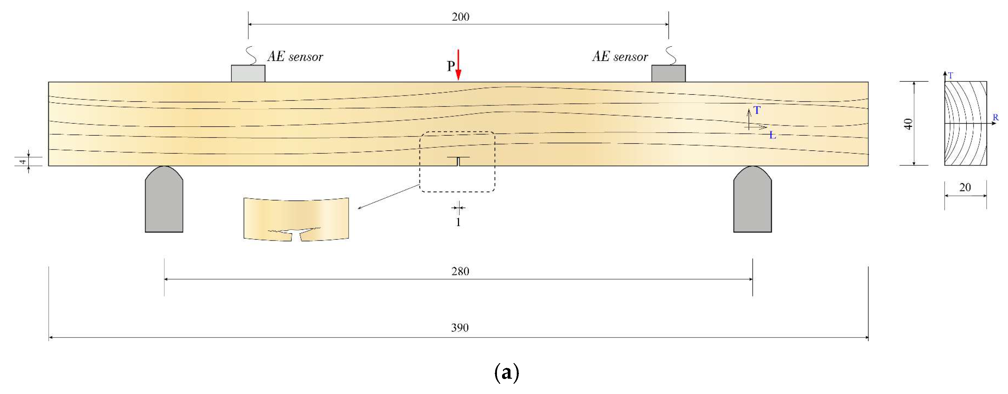
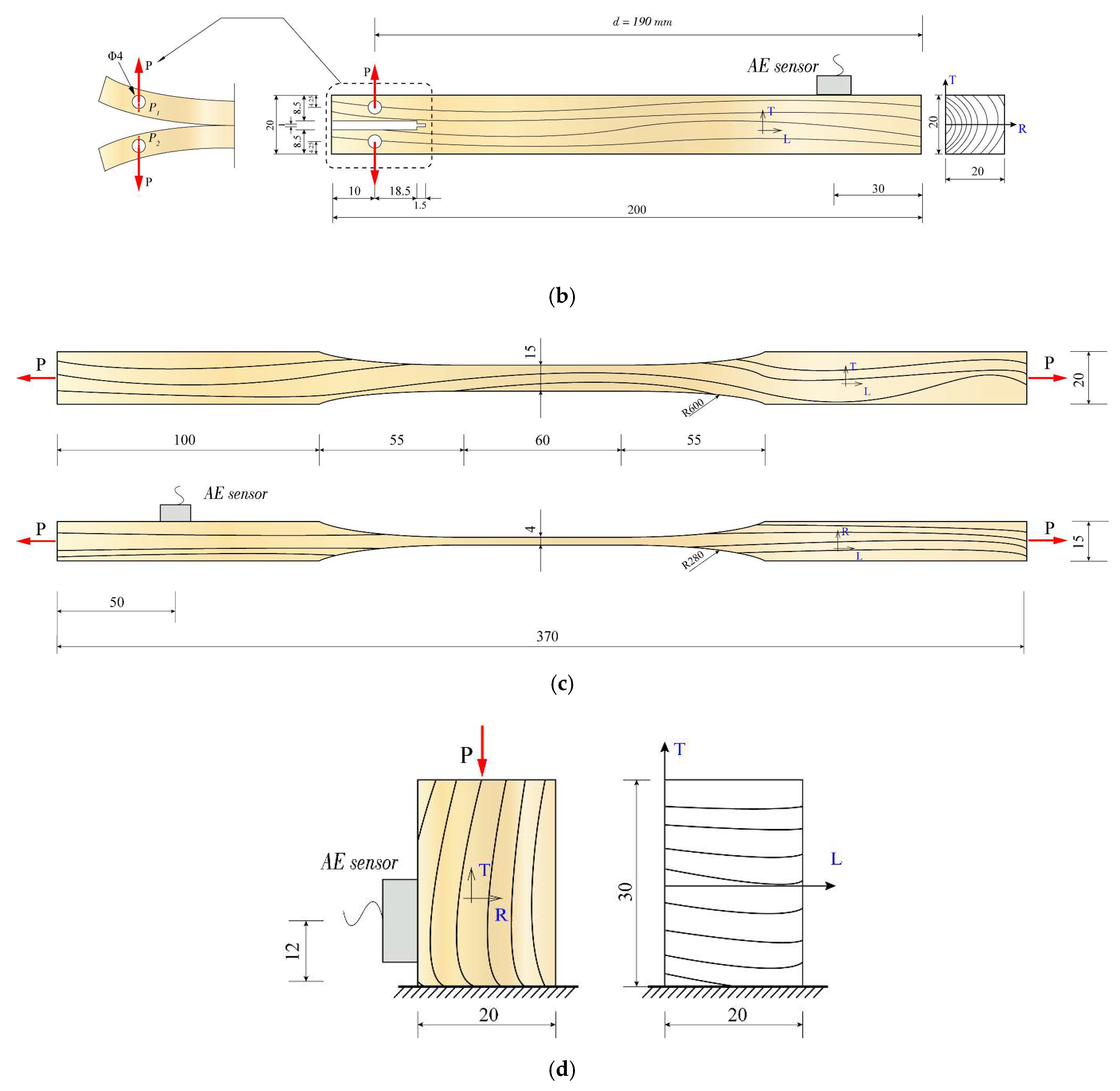
In this study, four types of tests were carried out, including double cantilever test, single bundle fiber tensile test, uniaxial compression test, and three-point bending test. The samples used were DCB sample, wood along grain tensile sample, wood cross-grain uniaxial compression sample, and three-point bending sample. The geometry, size, and sensor layout of the experimental sample are shown in Figure 1 and Table 1. The following are the fabrication methods of each of the four types of samples. The test samples were sawn into rectangular blank parts of different sizes in the first step. To process the wood cross-grain uniaxial compression sample, the blank was sawn into 20 mm (radial) × 20 mm (tangential) × 20 mm (longitudinal) and then the sample was made. To machine the DCB sample, the blank was sawn into 20 mm × 20 mm × 50 mm, then an 18.5 mm (longitudinal) × 3 mm (width) crack along the longitudinal direction was sawn at the center of the left side of the blank. After that, a 1.5 mm × 1 mm prefabricated crack along the L direction was cut out by a sharp blade. Finally, a hole with a diameter of 4 mm was drilled at the center of the two divided cantilevers. To process wood along the grain tensile sample, the blank was sawn into 15 mm × 20 mm × 370 mm; then, the blank was roughened into the specified arc shape with a saw. Then, a file was used to grind the arc at the connection of two planes into a fillet with a diameter of 600 mm in the tangential direction and a diameter of 280 mm in the radial direction. To machine the three-point bending sample, the blank was sawn into 20 mm × 40 mm × 370 mm, and then a 3 mm × 1 mm crack along the tangential direction was sawn at the center of the bottom plane. On this basis, a 1 mm × 1 mm prefabricated crack along the tangential direction was cut out by a sharp blade. Finally, the surface of all samples was polished smooth, and the samples were made. The installation position of the AE sensor used in each test is shown in Figure 1.
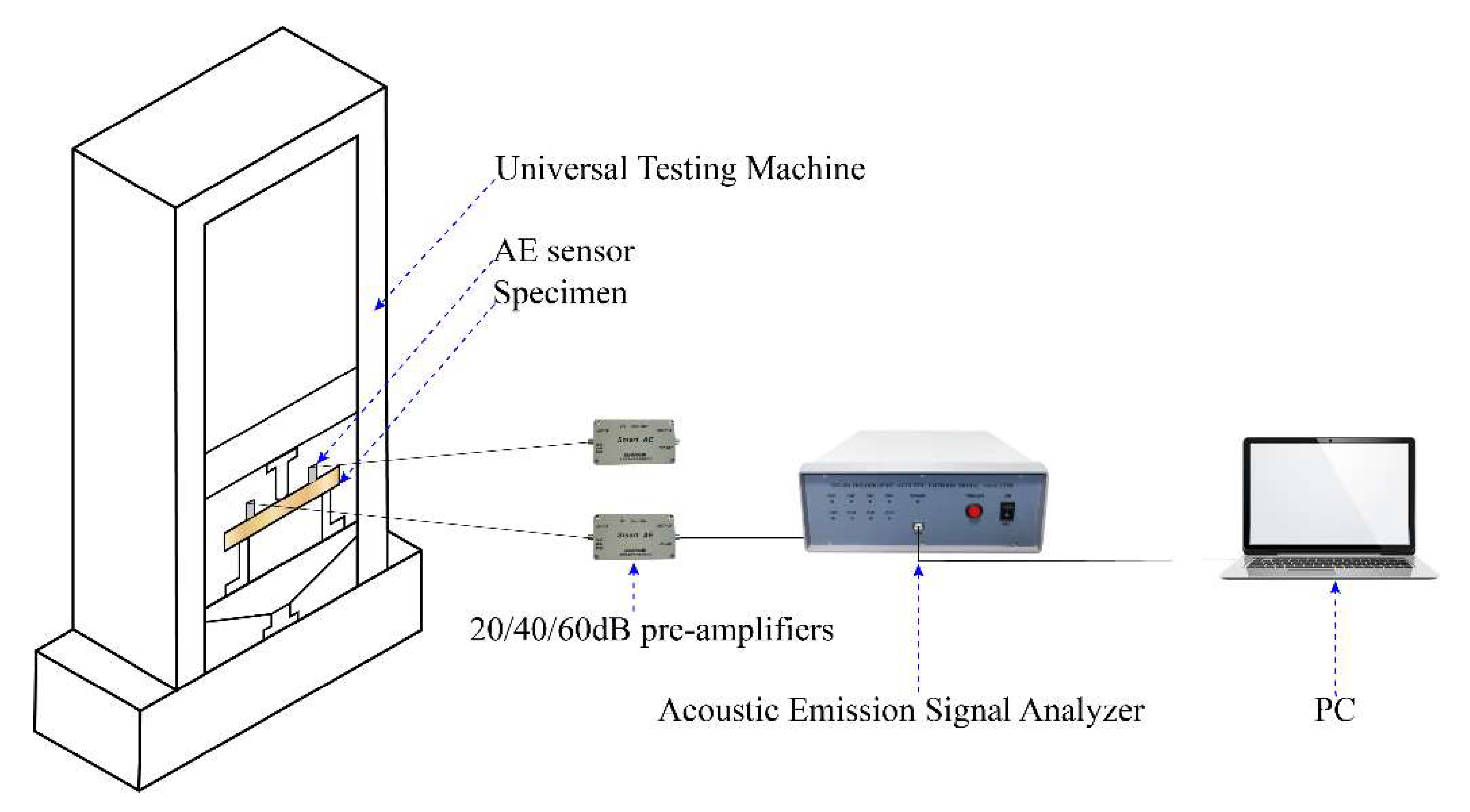
As shown in Figure 2, the test device is composed of a loading system and AE system. The loading system is produced by the universal mechanical testing machine (Reger, Shenzhen Reger Co., Shenzhen, China) and its maximum load is 10 kN. In order to reduce the friction noise between the loading head and the wood beam, a certain load shall be preloaded before the test. The testing machine operates in displacement-controlled mode, the loading rate is 0.001 m/min, and the computer draws the displacement of the loading timecurve. The AE data acquisition system produced by China Soft Island Company is used to record AE activities. The AE sensor employed is an RS-2A acoustic emission sensor with an acquisition frequency range of 50–900 kHz. The signal is pre-amplified by the pre-amplifier and input into the AE signal analyzer, and the gain of the pre-amplifier is 40 dB. Silicone grease is used to obtain good acoustic coupling on the sensor surface. Considering the environmental noise, a threshold of 30 dB is adopted, and the duration is less than 20 μS signal and detected mechanical and motor noise is screened in AE parameter analysis. Because the wood damage mode produced in the three-point bending experiment is complex, the sampling rate of 2.5 MHz is adopted to prevent the loss of important data, and the sampling rate of the other three types of experiments is 1 MHz/s, so as to ensure the recording of all sensor output data. For each AE event, the data acquisition system monitors the amplitude of the signal in real time. All other parameters (peak frequency, energy, duration, etc.) are counted according to the waveform.
3. Results and Analysis
The accurate and scientific analysis of AE characteristics is of great significance to explain the failure mechanism and damage deterioration of wood. The distribution of AE parameters reflects the relationship between the AE characteristics of wood and the control failure mechanism. The direction of wood fiber relative to the force direction defines the potential main failure modes: microcrack damage, cell wall buckling and collapse, interlayer cracking, fiber fracture, and fiber pullout. In order to establish the mapping law, the following discussion focuses on the failure analysis of four types of wood damage experimental material samples. The experimental results adopt representative AE signal characteristic parameters, including energy, amplitude, and peak frequency.
3.1. Three-Point Bending Test
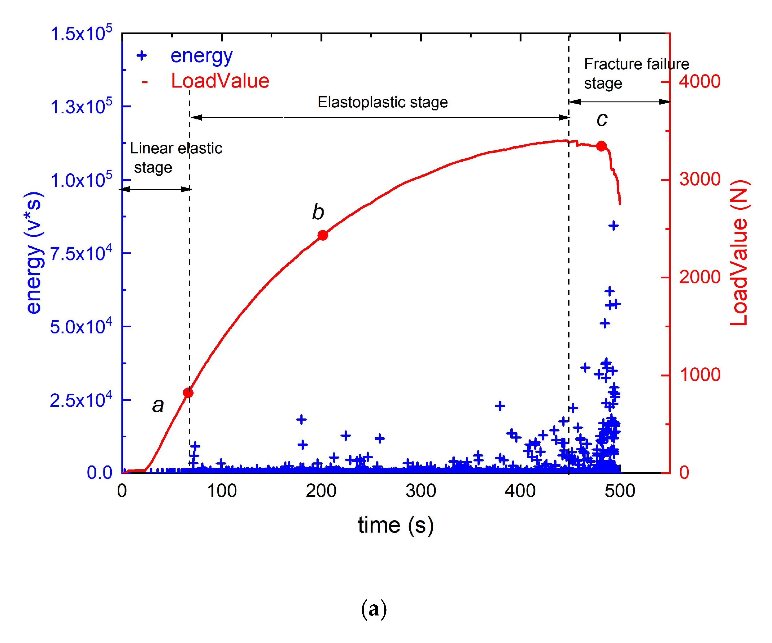
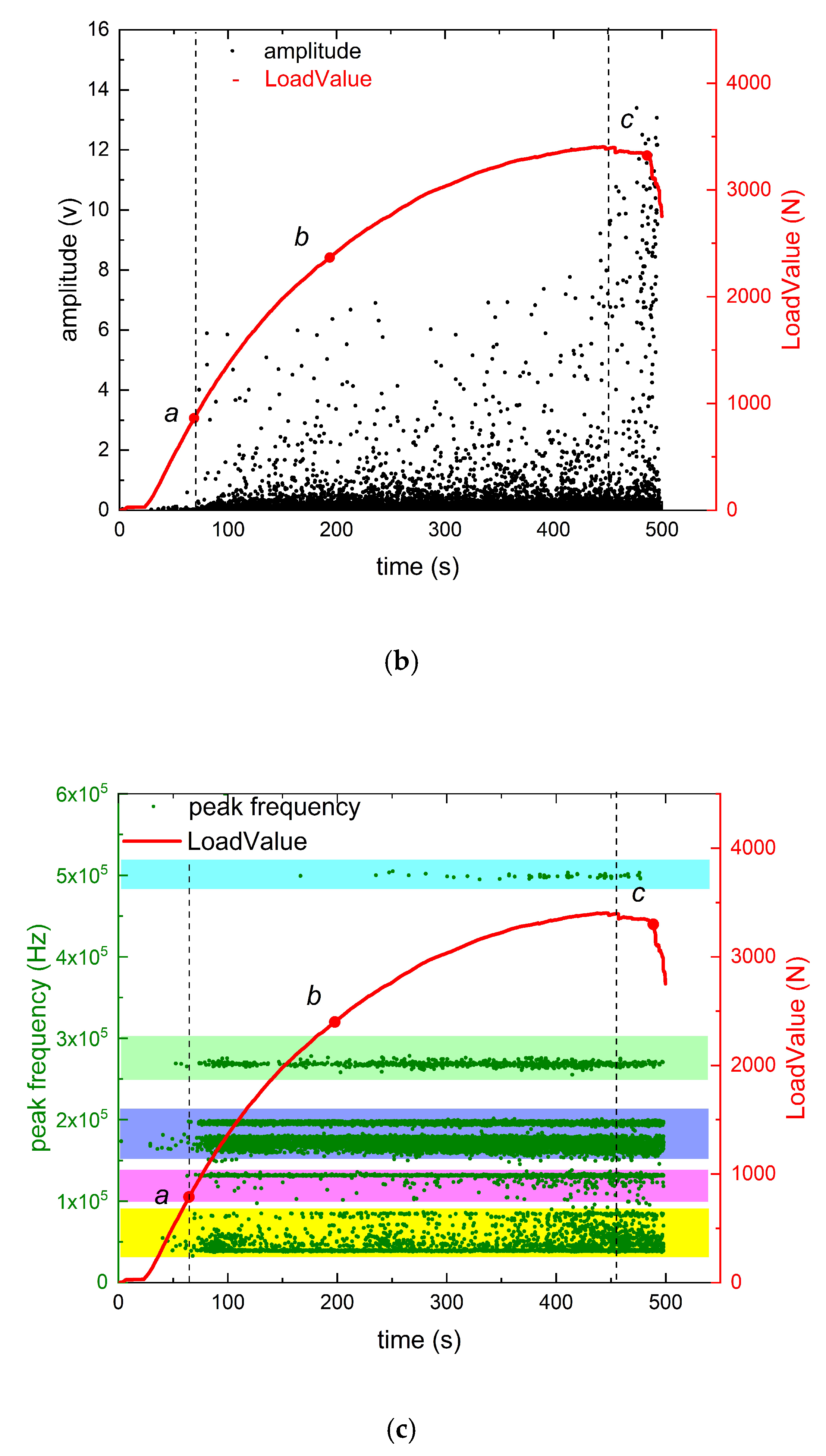
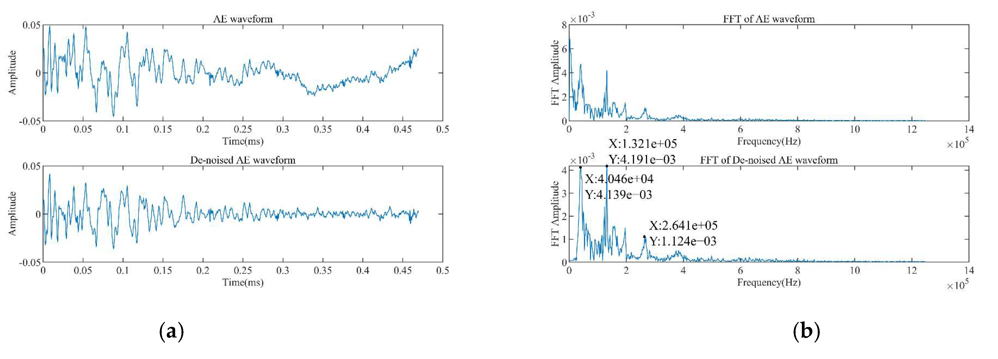
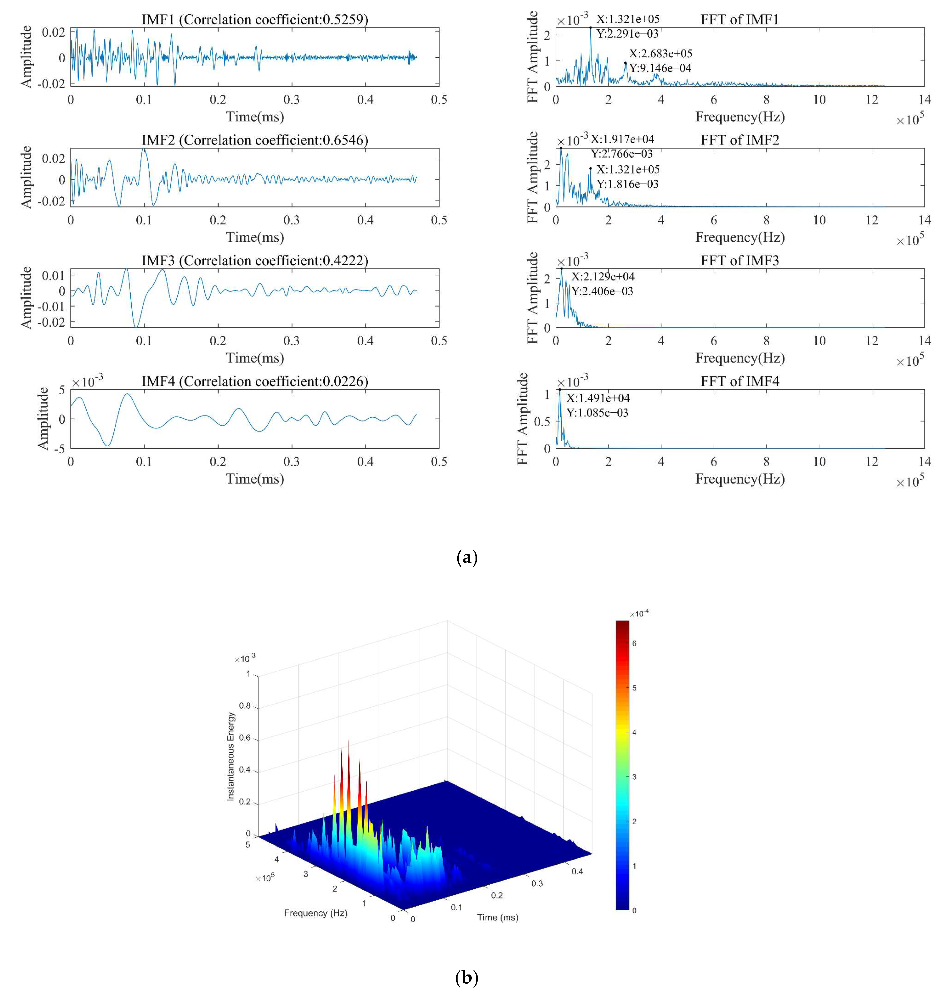
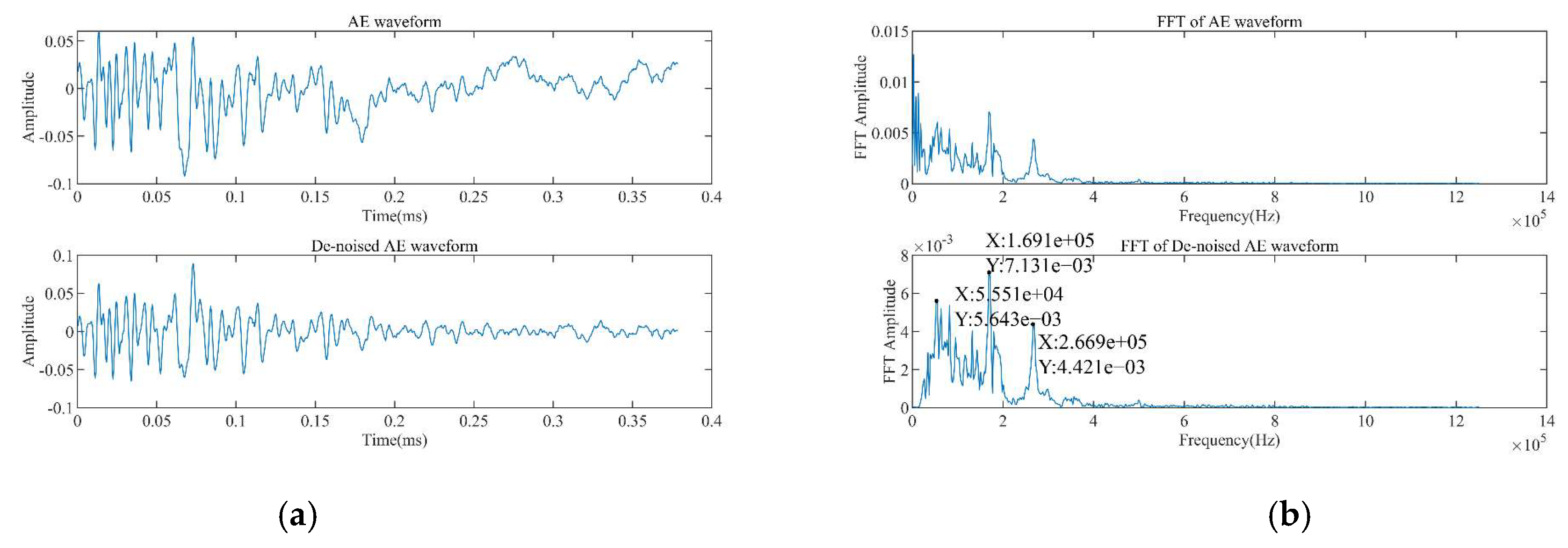
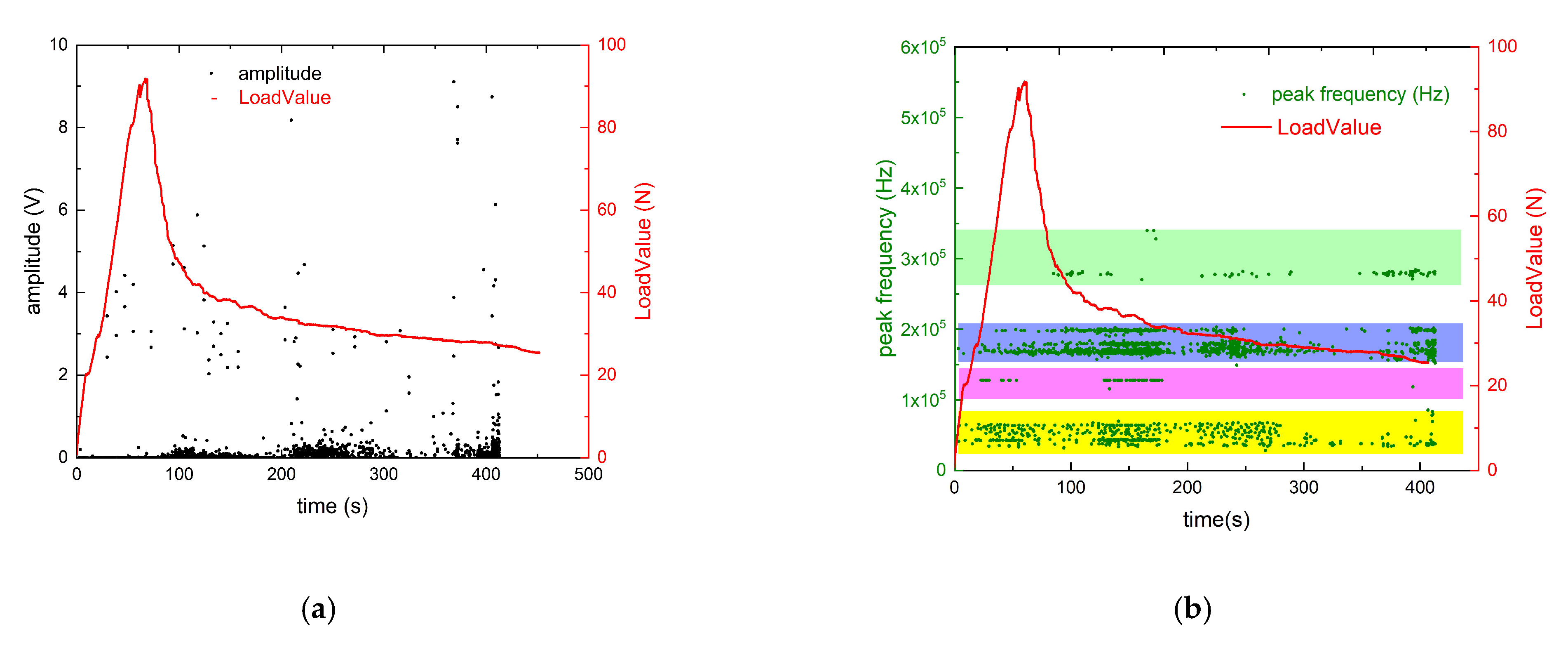
Figure 3 shows the variation of load and AE signal amplitude, energy, and peak frequency of three-point bending specimen S0 with time. It is obvious from Figure 3 that the whole three-point bending test is divided into three stages. In the first stage: (0–75.2 s) linear elastic stage, no obvious AE signal is generated. There is a turning point, a, on the load time curve at 75.2 s. Generally speaking, when the prefabricated transverse crack wood beam is subjected to bending load, the wood crack initiation occurs at the critical point of the linear elastic stage and non-linear stage, and the matrix microcrack starts at low stress level and will not affect the material properties [15]. The initiated crack will propagate along the fiber direction, and the damage mode is the same as that of interlaminar cracking. The AE signal is selected to perform fast Fourier transform at time a (75.2 s). At the same time, considering the influence of environmental noise on the experimental results, the waveform is filtered and denoised. The waveform and fast Fourier transform results of the AE signal after noise reduction are shown in Figure 4. It can be seen from the figure that the FFT power spectrum in this particular case presents multiple peaks, mainly focusing on two peak frequencies: 19 kHz and 132 kHz. The FFT power spectrum can be used as the fingerprint of damage events, so it can be used as a means to distinguish them. Then, the empirical mode decomposition algorithm is used to decompose the AE signal into multiple modal components, and Hilbert–Huang transform (HHT) is carried out on this basis. The IMF1–4 waveforms and 3D joint time-frequency diagram of the AE waveform are shown in Figure 5. The drawing of the 3D joint time-frequency diagram is based on the EMD and HHT of AE signal. In this study, the frequency sampling time-instantaneous energy diagram is applied, which can clearly display the frequency distribution of the AE signal in the time domain. It can be seen from Figure 5 that the AE signal at time a basically includes only two signal components, which may correspond to two specific damage modes.
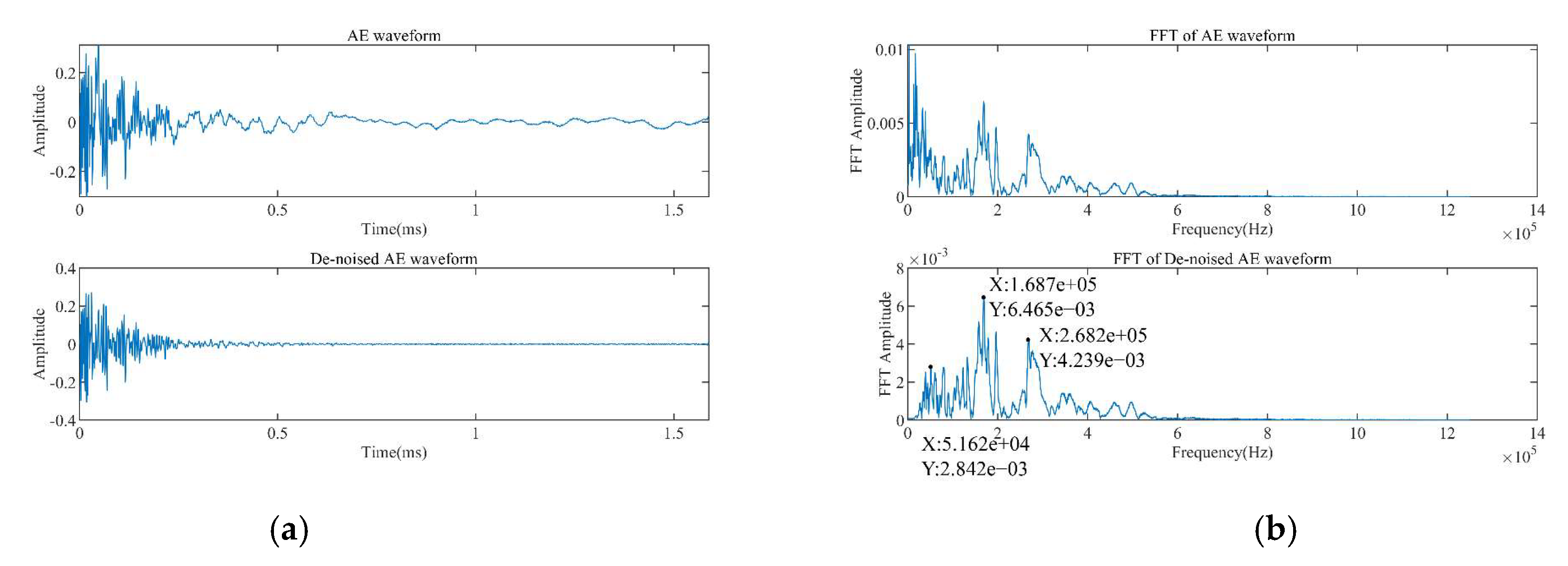
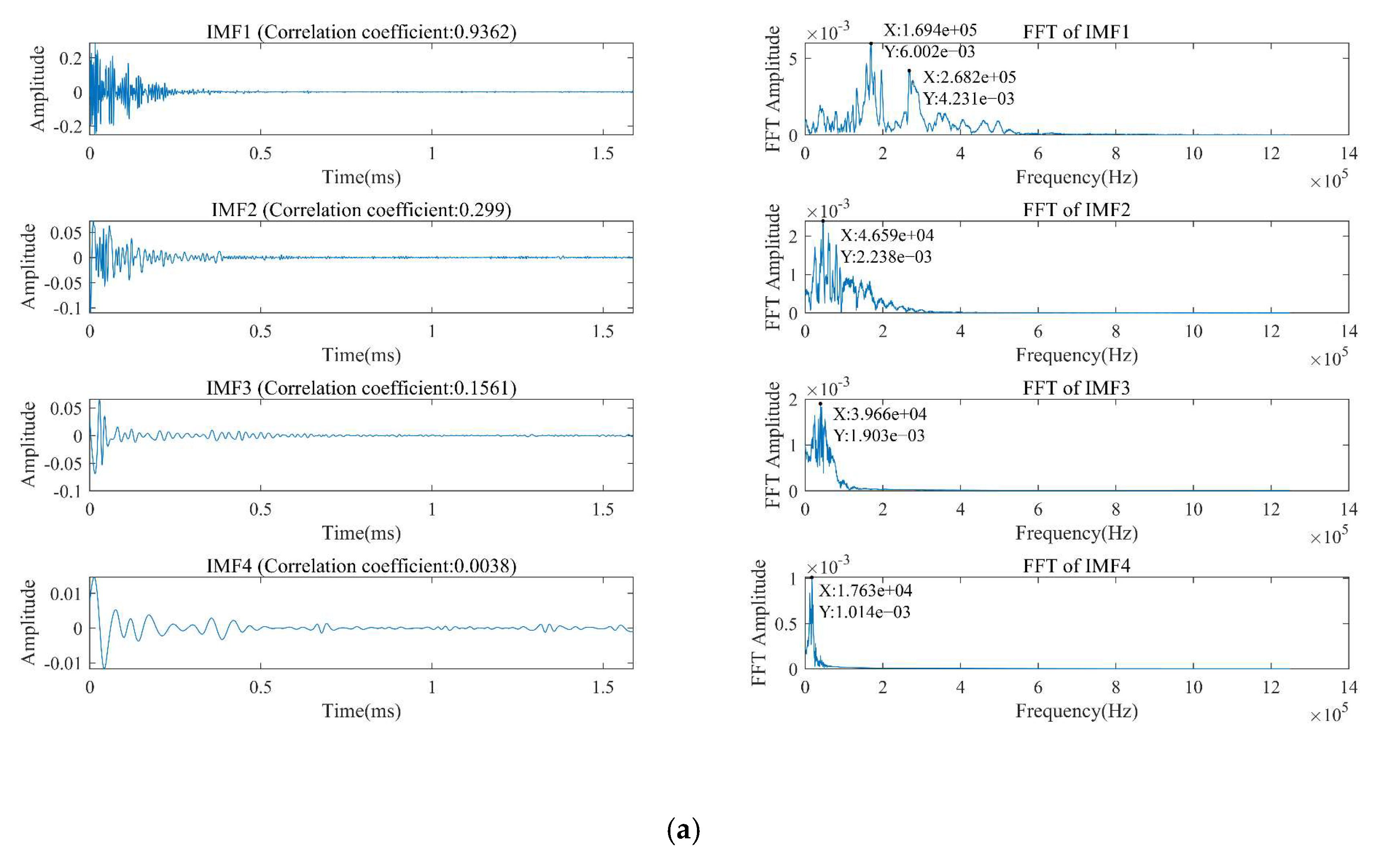
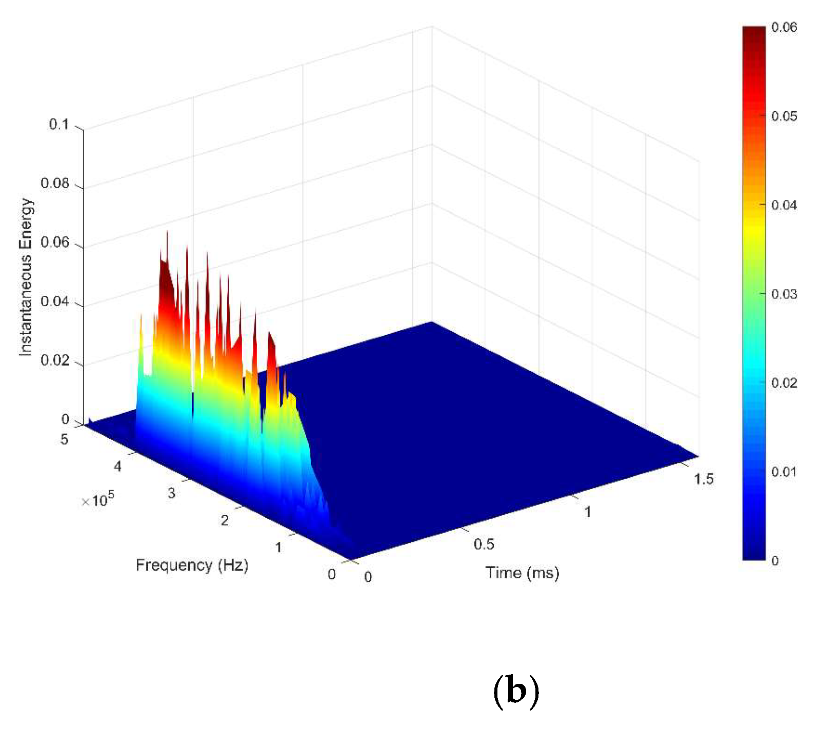
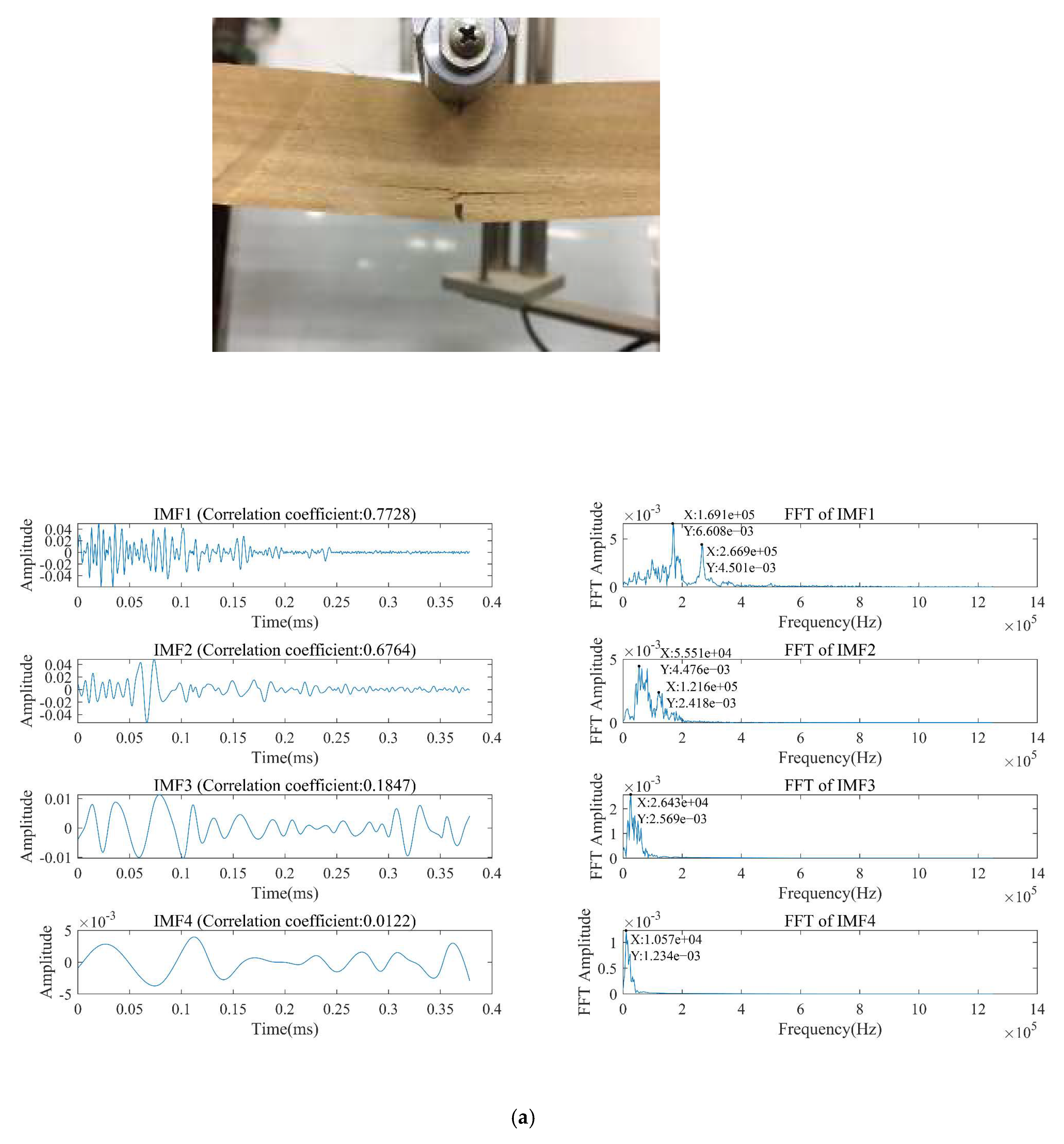
The second stage is the elastic-plastic stage (75.2–454.6 s), and the load time curve is non-linear. A large number of AE signals with low amplitude (1–8 V) and low energy value (0–25,000 V*s) are generated successively. The peak frequency content of most AE signals in the range of 40–300 kHz is shown in Figure 3c. At this stage, the damage inside the wood is further accumulated and degraded, the longitudinal crack perpendicular to the load direction occurs on the surface of the wood beam, and the compression zone is deformed. Figure 6 shows the waveform and frequency domain analysis that results at selected time b (242.64 s). To distinguish the damage modes contained in the AE signal, the AE signal is decomposed into several IMF, and the IMF components waveform is analyzed by fast Fourier transform. The IMF1–4 waveforms and fast Fourier transform of the AE signal are shown in Figure 7a. Since the decomposed IMF component is a steady signal sequence, the peak frequency is selected as the main frequency of the IMF waveform, which is related to a specific damage mode. It can be seen that the dominant frequencies of each IMF waveform from high to low are 160, 46, 39, and 17 kHz, respectively, which may correspond to different damage modes of wood. In addition, it is obvious that the FFT of the internal mode IMF1 has two peaks, 169 and 268 kHz, respectively. The 3D joint time-frequency diagram of the AE waveform is shown in Figure 7b. It can be seen that the AE signal includes signal elements of multiple damage modes, and the main frequency ranges are 320–390 kHz, 140–190 kHz, and 30–70 kHz.
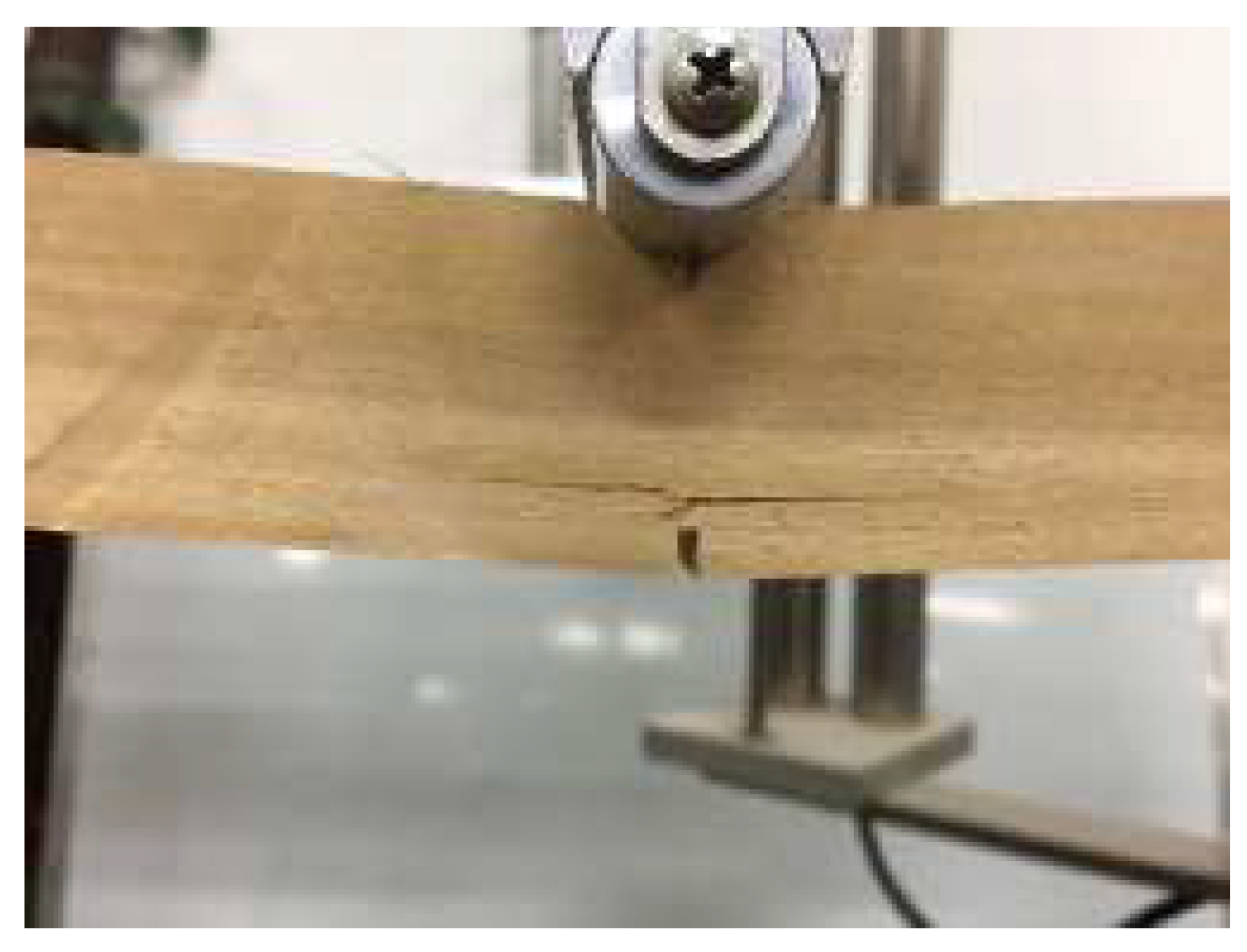
In the third stage (454.6 s–550.2 s), the load suddenly decreases, and there are obvious visible cracks on the surface of the wooden beam. The actual fracture diagram of sample S0 is shown in Figure 8. The amplitude and energy of the AE signal increase suddenly. Several obvious peak frequency ranges are observed, and peak frequency distribution is relatively concentrated in the ranges of 20–80 kHz, 100–130 kHz, 150–200 kHz, 250–290 kHz, and 470–500 kHz. In the last stage of the three-point bending test, with the emergence of a large number of secondary cracks in the tensile area, serious extrusion deformation also occurs in the compression area. The main failure forms of the sample may be cell wall buckling and collapse, longitudinal microcrack damage, interlaminar cracking, fiber fracture, and fiber bundle pullout. Generally speaking, cracking (longitudinal microcrack damage), interlaminar cracking, and fiber bundle fracture pullout provide a means for the final failure of the sample. At this stage, more kinds of damage modes occur than in the second stage in Figure 3c. Point c (493.06 s) AE signal is selected for fast Fourier transform and HHT analysis. The waveform and frequency domain analysis are shown in Figure 9. The IMF1–4 waveforms and fast Fourier transform of the AE signal are shown in Figure 10. It can be seen that the FFT power spectrum in this particular case shows several peaks, and the peak frequencies of AE signals are 169 khz and 268 khz. One possible explanation is that the waveform is superimposed by independent sources related to multiple damage modes, and each source has a frequency in an exclusive range.
3.2. Double Cantilever Beam Test (DCB)
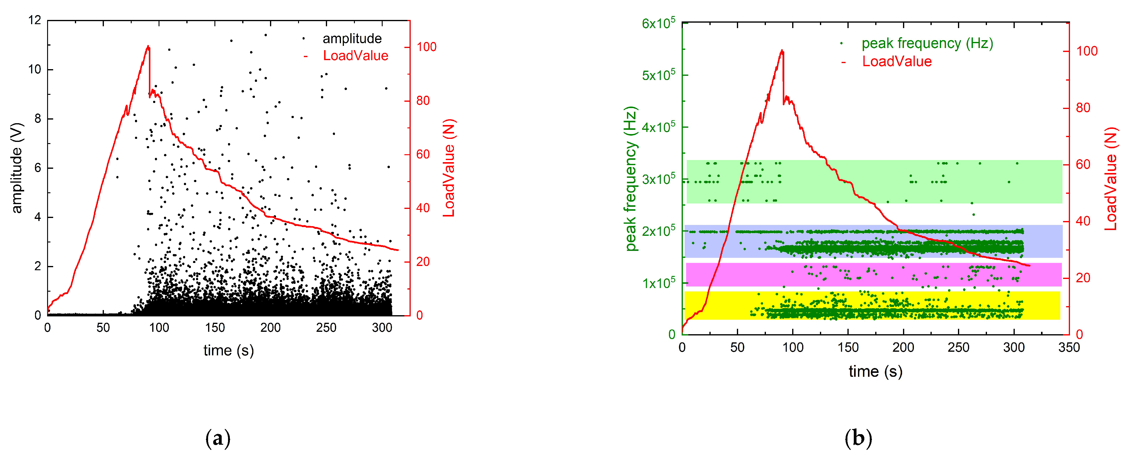
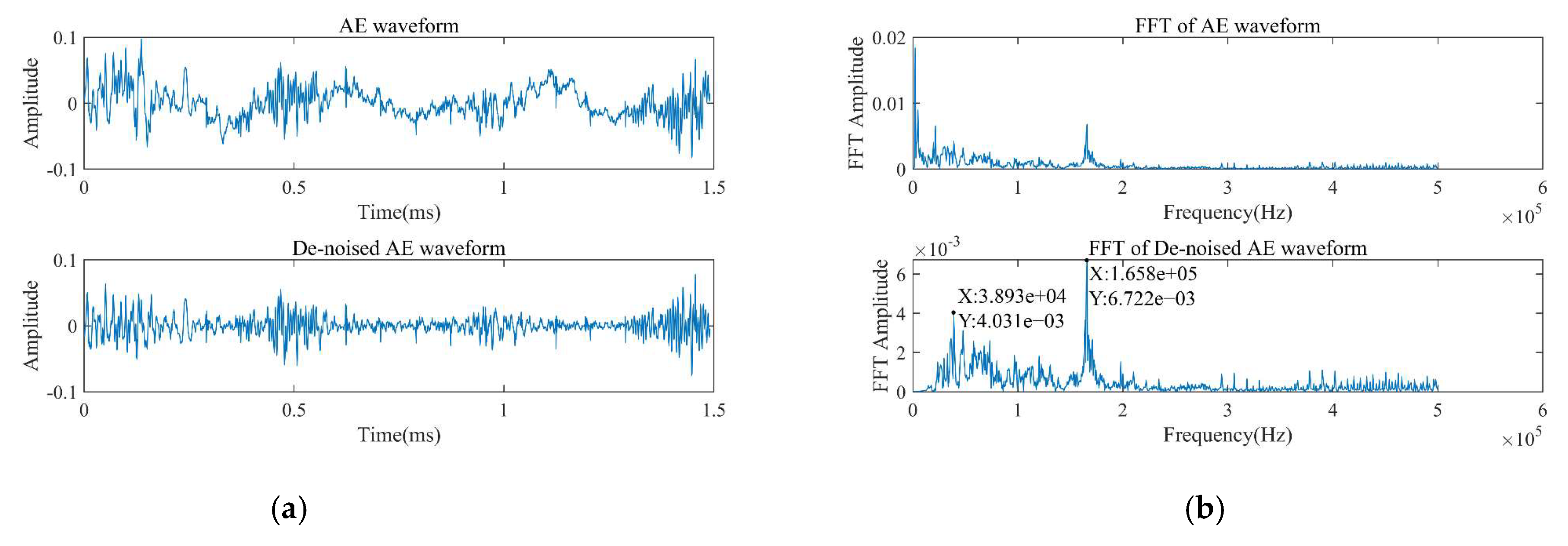
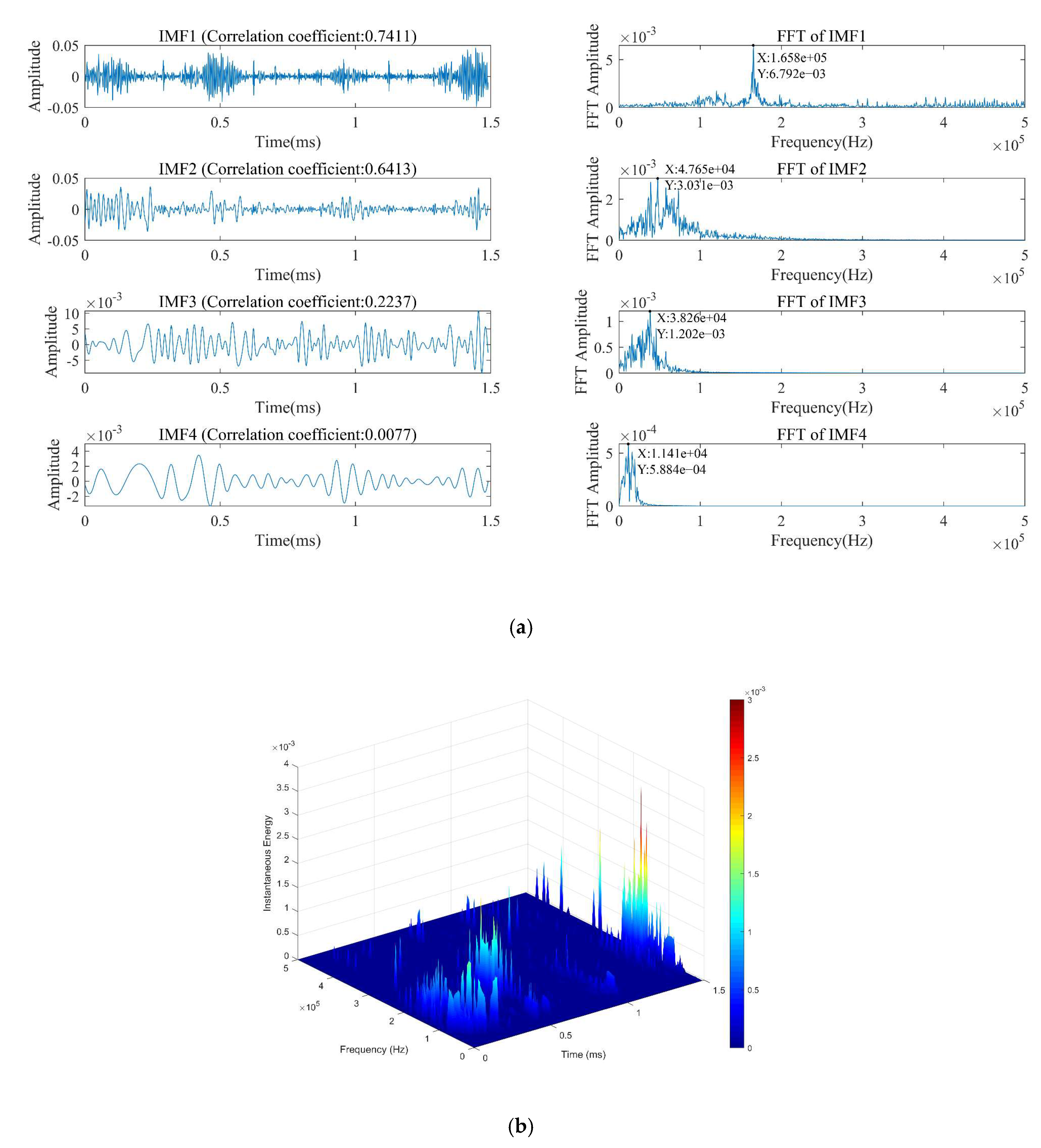
The double cantilever beam test is a typical interlaminar cracking characterization test. The double cantilever beam specimen (DCB) is manufactured in the form of pre-crack. It is obvious from Figure 11 that the loading process of the sample is divided into two stages: the first stage (0–97.89 s) 0. With the increase of load, the wood beam is in linear elastic deformation and produces almost no obvious acoustic signal. In the second stage (97.89–235 s), a large number of high-amplitude acoustic signals are generated, and the fibers in the material are constantly subjected to the tension perpendicular to the fiber direction to produce interlayer cracking. Delamination occurs obviously, resulting in cracking of the fiber interface. At 97.89 s, the load drops sharply, and the wood beam cracks along the grain rapidly. The damage mode is mainly interlayer cracking. The peak frequency is mainly concentrated in two intervals, ranging from 150–210 kHz and 20–80 kHz. The AE signal is selected for fast Fourier transform and HHT filtering in 90.865 s, as shown in Figure 12. It is observed that the fast Fourier transform power spectrum in this specific case presents double peaks, and the main peak frequency is 165.8 kHz. From Figure 13, the AE signal includes two or four signal components. The correlation coefficients of IMF1–4 are 0.7411, 0.6413, 0.2237, and 0.0077. The frequency range of IMF1 is 150–210 kHz and the frequency range of IMF2 is 20–80 kHz. It is a signal with lower amplitude. Therefore, the peak frequency range of 150–210 kHz may be relevant to interlaminar cracking.
3.3. Uniaxial Compression Test
Figure 14 shows the time history diagram of load value and amplitude and peak frequency of AE signal for specimen U1 in the uniaxial compression test. From the results, the whole test was divided into two stages. In the first stage (0–66 s), the AE amplitude is low and the main range of AE peak frequency is 30–80 kHz and 160–200 kHz. From 66 s after the start of the test, the high-amplitude AE signals began to appear.
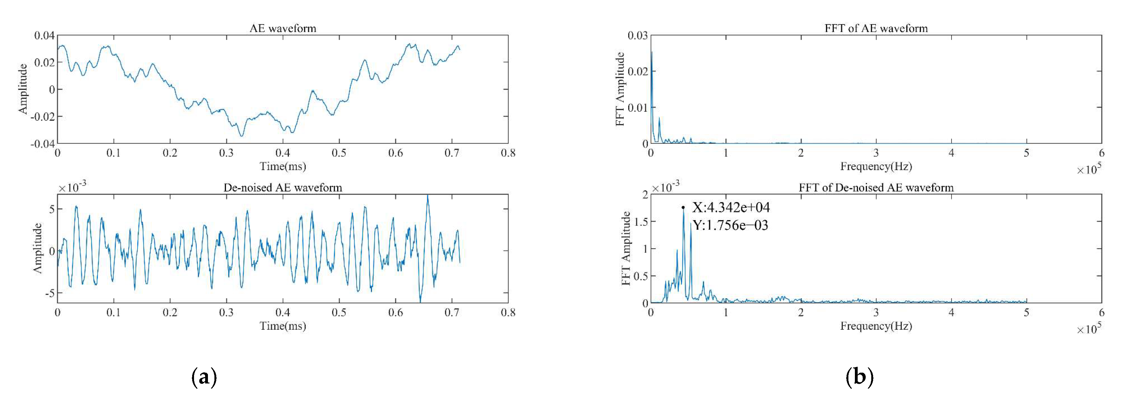
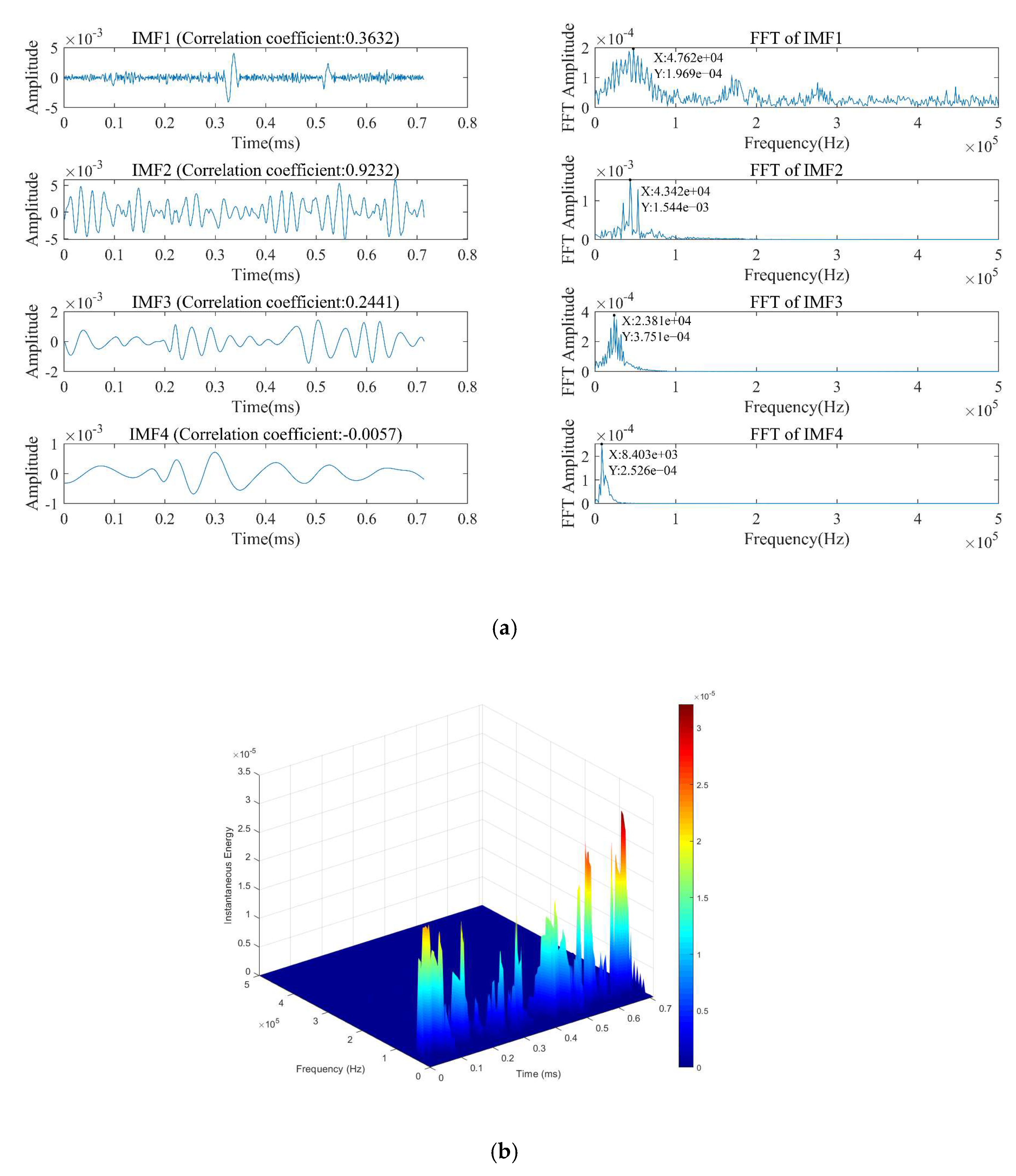
Based on the result of DCB test, the signal in the peak frequency range of 160–200 kHz is related to delamination; therefore, the signal with peak frequency of 30–80 kHz is mainly analyzed. One AE signal was chosen to perform FFT at 93.948 s; the waveform and FFT of the AE signal are shown in Figure 15. According to the observation, the FFT power spectrum of the AE signal has one peak at the time, and its peak frequency is 43.42 kHz. Figure 16 shows the frequency spectrum of the IMF component obtained after EMD decomposition, from which it can be obtained that the peak frequency of IMF1 is 47.62 kHz and the peak frequency of IMF2 is 43.52 kHz. Figure 13 shows the 3D time-frequency joint diagram of the signal, and it can be clearly seen that the instantaneous energy of signals with frequency in the range of 30–80 kHz is large, indicating that the relative intensity of these signal AE events is high. The results of literature [32] show that the main damage mode in the uniaxial compression test is the buckling and collapse of cell wall damage mode, so the signal in this frequency range may be related to the buckling and collapse of cell wall damage mode.
3.4. Fiber Bundle Tensile Test
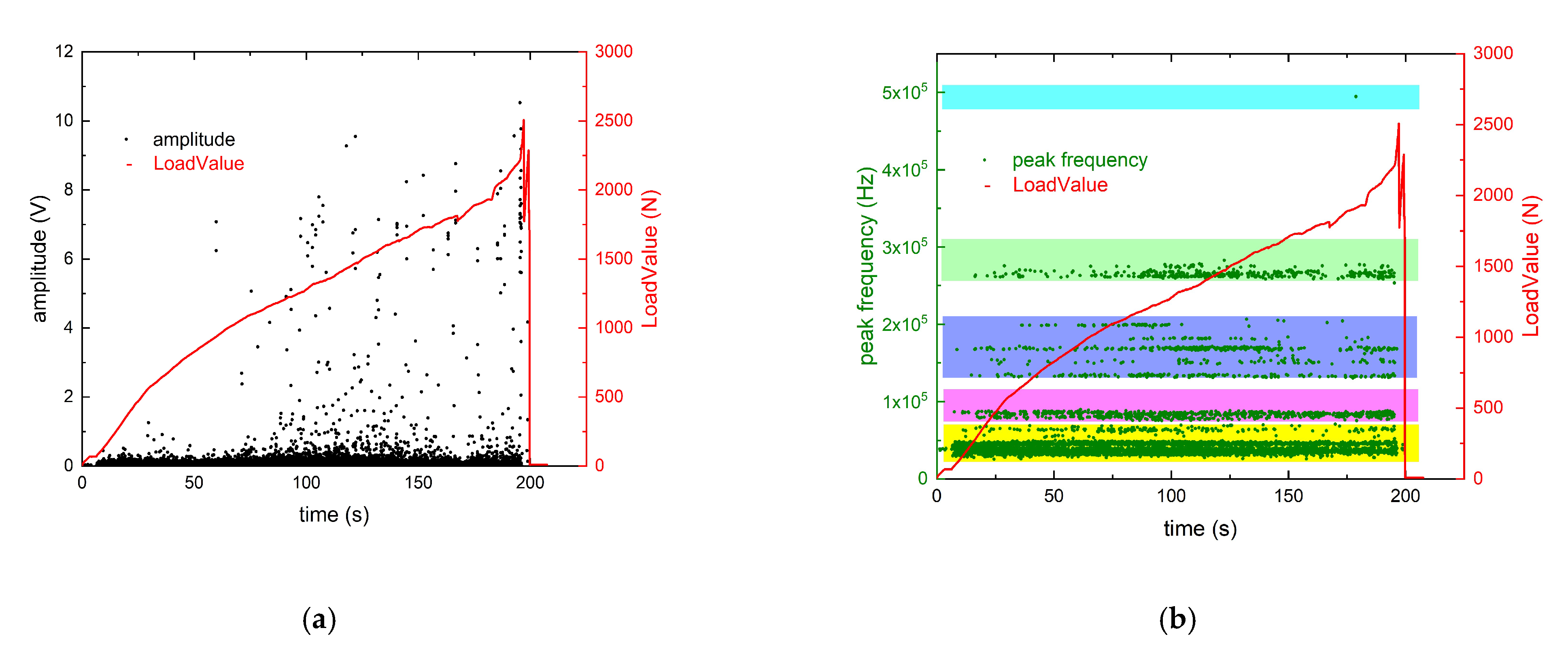
Figure 17 shows the variation of load value and amplitude and peak frequency of the AE signal with time for specimen T1 in the single bundle fiber breakage test. The whole test was divided into two stages from the result. In the first stage (0–80 s), the AE amplitude is low and the main range of AE peak frequency is 30–80 kHz. From 80 s after the test, the high-amplitude AE signals began to appear, and AE signals with peak frequency in the range of 250–270 kHz increased significantly. At 195 s, the test piece began to break, and the test ended at 200 s.
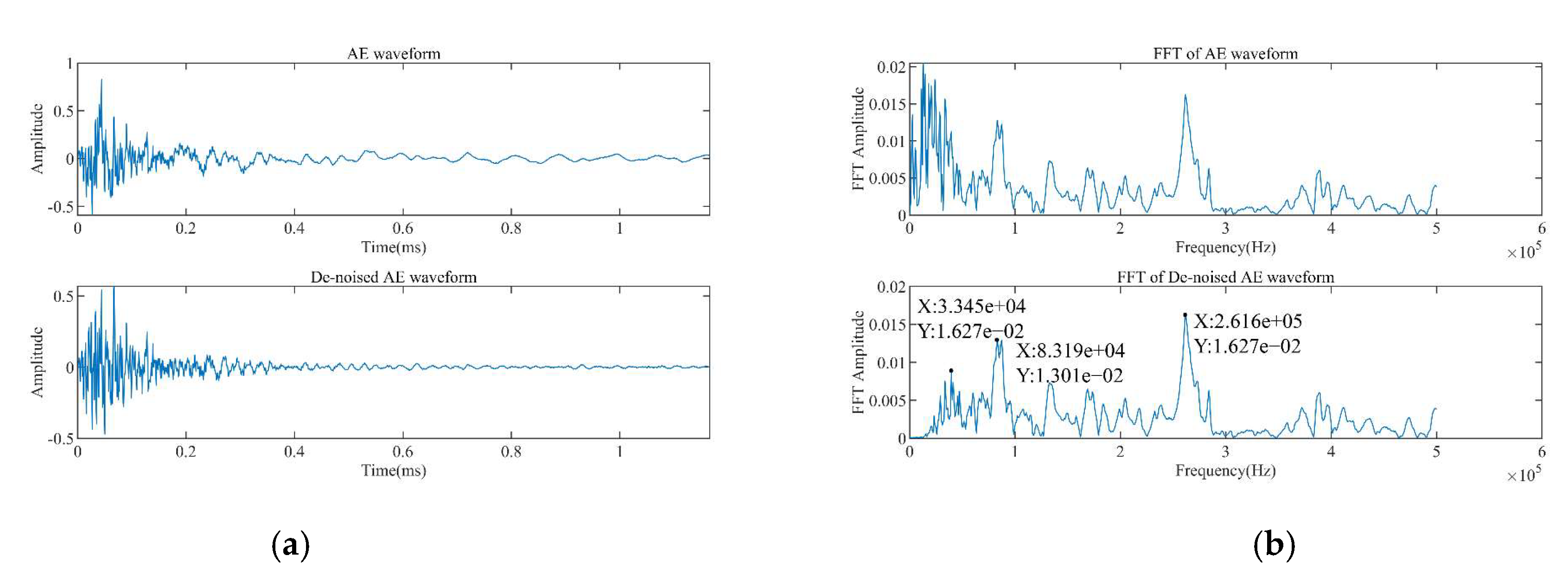
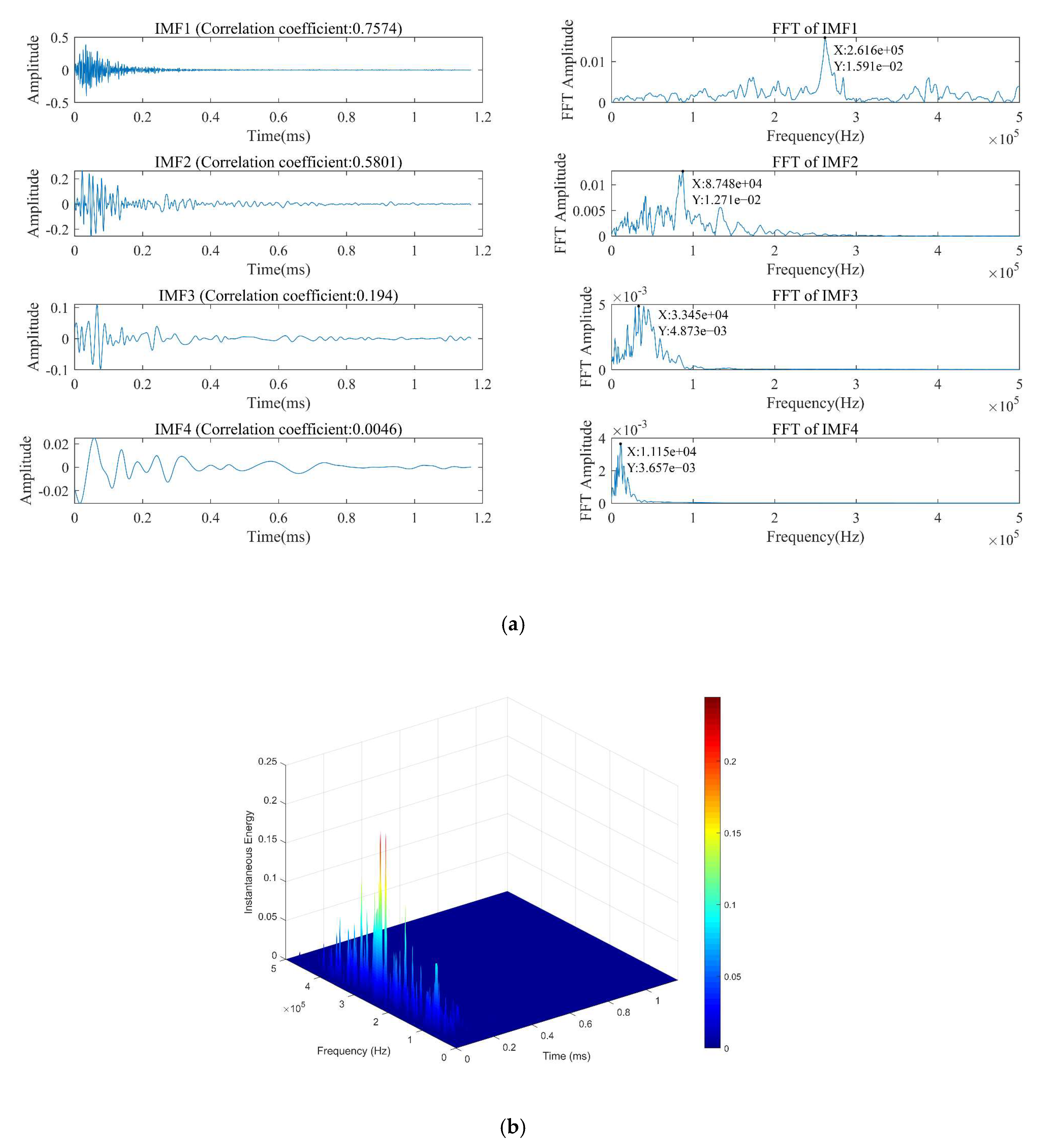
One AE signal was chosen to perform FFT at 194.995 s, because the specimen is pulled off at this time, and the fiber breakage damage mainly occurs. The waveform and FFT of the AE signal are shown in Figure 18. According to the observation, the FFT power spectrum of the AE signal has two peaks currently, and the main frequencies are 87 kHz and 261 kHz, respectively. In order to distinguish the main damage frequency, the signal is decomposed by EMD algorithm. The correlation coefficients between IMF1–4 and the original signal are 0.7574, 0.5801, 0.1940, and 0.0046, respectively. Therefore, the first three components are taken for analysis.
Figure 19a shows the frequency spectrum of the IMF component obtained after EMD decomposition, from which it can be obtained that the peak frequency of IMF1 is 261.16 kHz and the peak frequencies of IMF2 and IMF3 are 87.48 kHz and 33.45 kHz, respectively. Figure 19b shows the 3D time-frequency joint diagram of the signal, and it is obvious that the frequency of the AE signal in the range of 250–270 kHz is the most prominent.
In the second stage (after 80 s), the AE signal with peak frequency in the range of 250–270 kHz increases. Therefore, it can be inferred that the signals with peak frequency in the range of 250–270 kHz may be related to fiber breakage damage mode. It can thus be ascertained from the uniaxial compression experiment that the signals in the range of 30–80 kHz may be related to the matrix debonding damage.
4. Discussion
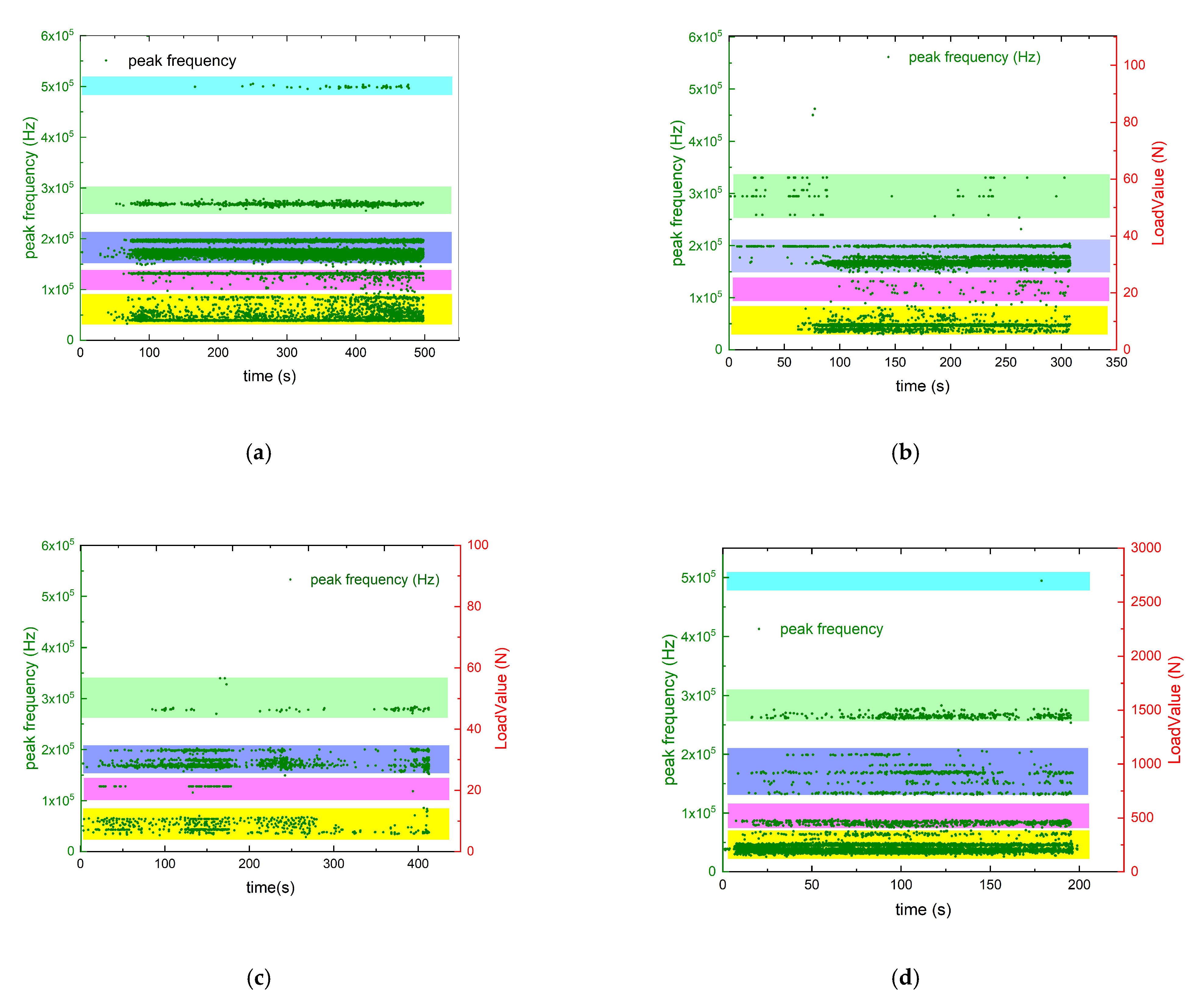
Standard bending, tensile, and compression tests including different main damage modes were carried out on wood samples, and AE events were recorded from these tests. In order to obtain the preferred damage mode, the fiber orientation of each group of samples was different. The main failure mechanisms of wood include cell wall buckling and collapse, interlaminar cracking, fiber fracture, microcrack damage, delamination, and fiber pullout. From the results of AE data of each sample, the amplitude and energy of the AE signal are difficult to be considered as the characteristics to distinguish the damage mode, and they are more suitable to reflect the damage evolution of wood. As shown in Figure 20, the statistical results reveal that the peak frequency content of different tests can be divided into five frequency bands, which may correspond to different damage modes. Five frequency bands are defined: (1) F1: 20–80 kHz; (2) F2: 90–140 kHz; (3) F3: 150–210 kHz; (4) F4: 250–350 kHz; (5) F5: 470–500 kHz.
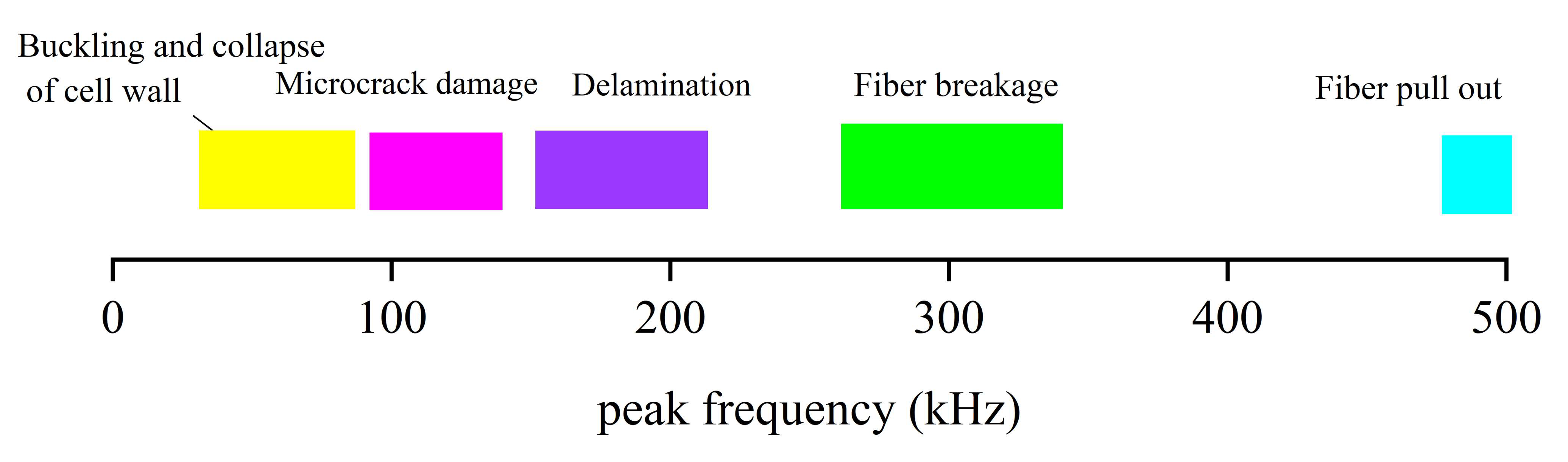
The three-point bending test of the prefabricated transverse crack wood beam in LT direction belongs to the composite fracture mode, and there is more than one damage mode in each stage of the fracture process. It can be seen from Figure 20a that the frequency band F1–F4 appears in the complete process of the three-point bending test, and the frequency band F5 begins to appear in the later stage of the test. In addition, since the main damage mode of the fiber bundle fracture test is fiber fracture, in Figure 20d, it can be seen that the F5 frequency band appears at the end of the fiber bundle fracture test, so the frequency band F5 may be related to the delamination and fiber pullout damage after fiber fracture. The main damage mode of the uniaxial compression test is cell wall buckling and collapse. According to the frequency domain analysis results of uniaxial compression reflected in Figure 15, the frequency domain of the AE signal is unimodal and belongs to frequency band F1. Therefore, frequency band F1 is related to cell wall buckling and collapse damage. It can be seen from Figure 20b that there is no obvious AE signal in the early stage of the DCB test, and the acoustic signal generated after the beginning of interlayer damage is mainly frequency bands F1 and F3. Therefore, it is speculated that the damage mode corresponding to F3 is interlayer cracking, which is accompanied by cell wall buckling and collapse damage in the compression area of wood beam during the test. The AE events of band F2 almost occur in most tests. In the uniaxial compression test, the acoustic signal of medium-frequency band F2 is relatively scarce. Because there must be a tensile zone in other bending and tensile tests except the uniaxial compression test, and the substrate cracking damage will inevitably occur when the stress in the tensile zone reaches the critical value, band F2 may thus correspond to the substrate cracking damage. Fiber fracture damage is one of the main damage modes in the fiber bundle tensile test. According to the literature [32], fiber fracture events usually occur at a higher frequency. The AE event in frequency band F4 in Figure 20d can correspond to fiber fracture damage. It should be added that due to the friction between the fixture and the sample of the fiber bundle tensile test, the frequency range of the AE event coincides with the frequency band F1. Therefore, the AE event in the medium-frequency band S1 in Figure 20d may partly come from the friction noise. Based on the above analysis, the peak frequency range corresponding to each damage mode is summarized as shown in Figure 21.
5. Conclusions
The objective of this study is to identify the damage mode of wood by the combination of bending, tension, compression, and AE technology. Therefore, samples with different fiber directions and loading directions are used to produce various damages in a controllable manner. During the test, specific damage modes may appear in a given specimen. Through the post-processing and analysis of AE signals collected in the test, such as filtering, denoising, and Fourier transform, the AE characteristics related to specific damage modes are obtained. In this study, EMD and HHT transform are used to separate and identify all damage modes in the composite signal. The main conclusions are as follows:
1. AE amplitude and energy can better reflect the damage evolution process of wood, but cannot effectively distinguish the failure mechanism. From the frequency domain analysis results of AE signals, it is found that the law of AE peak frequency corresponding to different failure modes of wood can be clearly distinguished. Therefore, the AE peak frequency is more suitable and can be used as an important parameter to identify and distinguish different failure modes, so as to further identify different damage modes of wood.
2. The AE signal generated in the wood fracture process is often a composite damage signal, which contains more than one damage mode. The AE characteristics corresponding to different damage modes can be separated and extracted by EMD algorithm and FFT transformation. The peak frequency intervals corresponding to different damage modes are: (1) buckling and collapse of cell wall: 20–80 kHz; (2) microcrack damage: 90–140 kHz; (3) delamination: 150–210 kHz; (4) fiber breakage: 250–350 kHz; (5) fiber pullout: 470–500 kHz.
3. The Hilbert spectrum obtained by the HHT transformation of the AE signal can describe the variation law of instantaneous energy with frequency versus time. The frequency distribution on time scale can be clearly displayed on the 3D time-frequency joint graph of the AE signal, and the frequency content of the AE signal with different damage modes can be clearly distinguished.
In conclusion, the peak frequency of AE seems to provide an effective way to characterize the damage mode of wood. However, due to the special fiber structure in wood and the actual working conditions, the load direction is complex. The damage modes contained in AE signals may further increase. HHT transformation provides a promising method for feature extraction of AE signals of different damage modes of wood. Our future work will focus on further understanding the failure mechanism and crack evolution law of wood materials, and realizing the function of real-time in situ monitoring and identification of damage modes through HHT.
Author Contributions
D.Z. and J.Z. (Jian Zhao) conceived this study, J.Z. (Jianzhong Zhang) and J.T. conducted the experiments. J.T. and L.Y. implemented and analyzed the experimental results. J.T. and J.Z. (Jian Zhao) wrote the manuscript. All authors have read and agreed to the published version of the manuscript.
Funding
This research was funded by the Fundamental Research Funds for the Central Universities, Project Number 2021ZY67.
Conflicts of Interest
The authors declare no conflict of interest.
Appendix A. Fundamental Principles of HHT
The main contents of HHT transformation are divided into two parts: (1) empirical mode decomposition (EMD); (2) Hilbert transform. According to the time characteristics of the signal itself, the original signal is decomposed into multiple intrinsic mode functions (IMF). After Hilbert transform processing, the instantaneous frequency and instantaneous amplitude distribution of the component signal can be obtained, and then the time spectrum of the original vibration signal can be obtained.
Appendix A.1. Empirical Mode Decomposition (EMD)
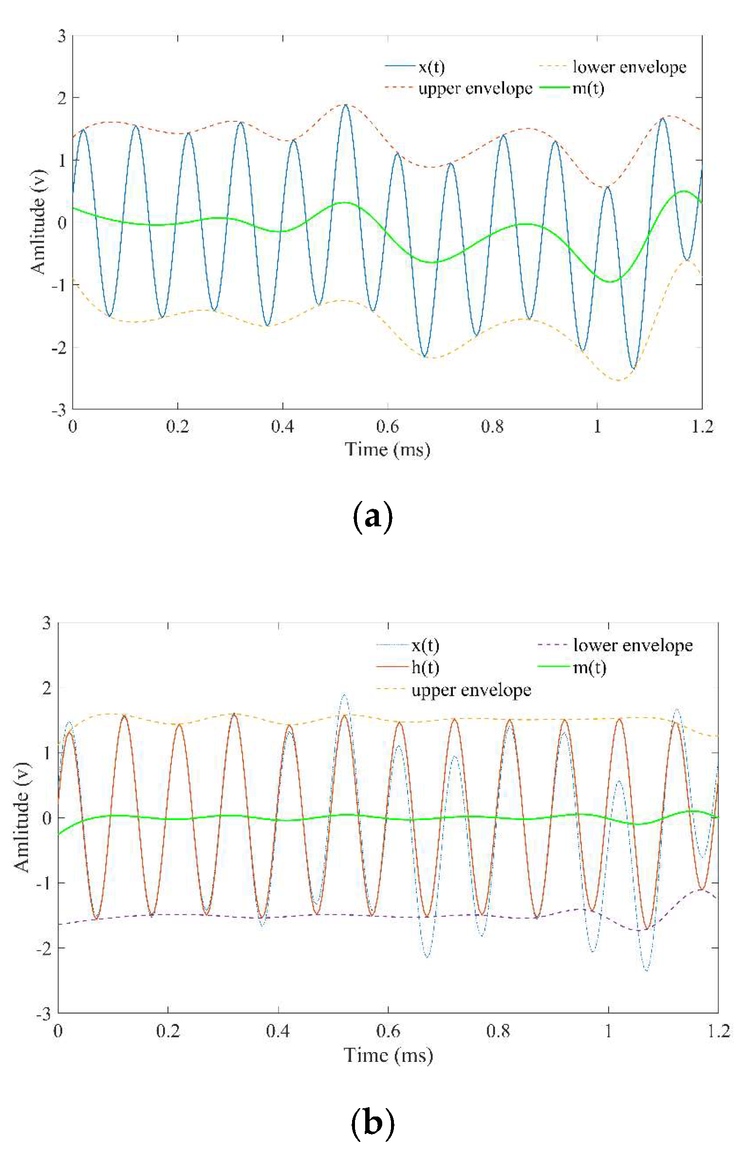
It is assumed that any complex signal is composed of some simple, different, and non-sinusoidal intrinsic mode function components (IMF). Each intrinsic mode function can be linear or non-linear. Two conditions shall be met [12]: a. the sum of extreme points and the number of zero crossings are the same or at most one difference; b. at any point, the mean value of the upper and lower envelope determined by the local maximum point and the local minimum point is zero.
Figure A1.
(a) Original signal x (t) and average envelope m (t) (thick line), upper and lower extremum envelope; (b) signal h_1 (t) in the sifting process.
Figure A1.
(a) Original signal x (t) and average envelope m (t) (thick line), upper and lower extremum envelope; (b) signal h_1 (t) in the sifting process.

① As shown in Figure A1, let the original signal be , first find all the extreme points on . Then the maximum point of is interpolated by cubic spline function curve to fit the upper envelope of the maximum point of the original signal. Then the minimum of is interpolated to fit the lower envelope of the minimum point, and the average envelope is recorded as .
② Let , judge whether the new time series meets the IMF conditions. If it is true, record as the IMF1 component. Otherwise, treat as a new signal and repeat the above process.
③ Remove the IMF component from the original signal as a new original signal, repeat step ② until the limiting conditions are met, and finally decompose the IMF components of each order. Finally, the original signal is decomposed into the sum of each order IMF component and residual component, , i.e.:
Appendix A.2. Hilbert Transform
Firstly, the EMD method is used to decompose the signal into several eigenmode components, and then Hilbert transform is performed on each mode component to obtain the instantaneous frequency with practical physical significance. The calculation of Hilbert transform for each modal component is as follows:
where represents the eigenmode component, i = 1, 2 ... N; represents time; is the time interval.
The analytical signal for each modal component is constructed as follows:
where is the amplitude function; is the phase function; is an imaginary number.
The instantaneous frequency obtained by differential processing of the phase function is:
Then, the Hilbert spectrum of signal x (t) can be expressed as:
where R represents a real number.
The instantaneous energy of Hilbert is obtained by integrating the square of amplitude with frequency. The specific expression is:
References
- Maier, D. Building Materials Made of Wood Waste a Solution to Achieve the Sustainable Development Goals. Materials 2021, 14, 7638. [Google Scholar] [CrossRef] [PubMed]
- Wu, Y.; Shao, Z.P.; Wang, F.; Tian, G.L. AE characteristics and felicity effect of wood fracture perpendicular to the grain. J. Trop. For. Sci. 2014, 26, 522–531. Available online: https://0-www-jstor-org.brum.beds.ac.uk/stable/43150938 (accessed on 12 October 2014).
- Xu, P.; Guan, C.; Zhang, H.; Li, G.; Zhao, D.; Ross, R.J.; Shen, Y. Application of Nondestructive Testing Technologies in Preserving Historic Trees and Ancient Timber Structures in China. Forests 2021, 12, 318. [Google Scholar] [CrossRef]
- Sen, N.; Kundu, T. A new wave front shape-based approach for acoustic source localization in an anisotropic plate without knowing its material properties. Ultrasonics 2018, 87, 20–32. [Google Scholar] [CrossRef] [Green Version]
- Yin, S.X.; Cui, Z.W.; Kundu, T. Acoustic source localization in anisotropic plates with “Z” shaped sensor clusters. Ultrasonics 2018, 84, 34–37. [Google Scholar] [CrossRef]
- Zhao, X.M.; Jiao, L.L.; Zhao, J.; Zhao, D. AE attenuation and source location on the bending failure of the rectangular mortise-tenon joint for wood structures. J. Beijing For. Univ. 2017, 39, 107–111. [Google Scholar]
- Ye, G.Y.; Xu, K.J.; Wu, W.K. Multivariable modeling of valve inner leakage AE signal based on Gaussian process. Mech. Syst. Signal Process. 2020, 140, 106675. [Google Scholar] [CrossRef]
- Liu, C.; Wu, X.; Mao, J.L.; Liu, X.Q. AE signal processing for rolling bearing running state assessment using compressive sensing. Mech. Syst. Signal Process. 2017, 91, 395–406. [Google Scholar] [CrossRef]
- Butterfield, J.D.; Krynkin, A.; Collins, R.P.; Beck, S.B.M. Experimental investigation into vibro-AE signal processing techniques to quantify leak flow rate in plastic water distribution pipes. Appl. Acoust. 2017, 119, 146–155. [Google Scholar] [CrossRef]
- Manterola, J.; Aguirre, M.; Zurbitu, J.; Renart, J.; Turon, A.; Urresti, I. Using AEs (AE) to monitor mode I crack growth in bonded joints. Eng. Fract. Mech. 2020, 224, 106778. [Google Scholar] [CrossRef]
- Wisner, B.; Mazur, K.; Perumal, V.; Baxevanakis, K.P.; An, L.; Feng, G.; Kontsos, A. AE signal processing framework to identify fracture in aluminum alloys. Eng. Fract. Mech. 2019, 210, 367–380. [Google Scholar] [CrossRef] [Green Version]
- Xu, J.; Wang, W.X.; Han, Q.H.; Liu, X. Damage pattern recognition and damage evolution analysis of unidirectional CFRP tendons under tensile loading using AE technology. Compos. Struct. 2020, 238, 111948. [Google Scholar] [CrossRef]
- Kharrat, M.; Placet, V.; Ramasso, E.; Boubakar, M.L. Influence of damage accumulation under fatigue loading on the AE-based helth assessment of omposite materials: Wave distortion and AE-features evolution as a function o damage level. Compos. Part A Appl. Sci. Manuf. 2018, 109, 615–627. [Google Scholar] [CrossRef]
- Bucur, V. The Acoustics of Wood (1995); CRC Press: Boca Raton, FL, USA, 2017. [Google Scholar] [CrossRef]
- Tu, J.; Zhao, D.; Zhao, J.; Zhao, Q. Experimental study on crack initiation and propagation of wood with LT-type crack using digital image correlation (DIC) technique and AE (AE). Wood Sci. Technol. 2021, 55, 1577–1591. [Google Scholar] [CrossRef]
- Clerc, G.; Sause, M.G.; Brunner, A.J.; Niemz, P.; van de Kuilen, J.W.G. Fractography combined with unsupervised pattern recognition of AE signals for a better understanding of crack propagation in adhesively bonded wood. Wood Sci. Technol. 2019, 53, 1235–1253. [Google Scholar] [CrossRef]
- Reiterer, A.; Stanzl-Tschegg, S.E.; Tschegg, E.K. Mode I fracture and AE of softwood and hardwood. Wood Sci. Technol. 2000, 34, 417–430. [Google Scholar] [CrossRef]
- Zhao, Q.; Zhao, D.; Zhao, J. Thermodynamic Approach for the Identification of Instability in the Wood Using AE Technology. Forests 2020, 11, 534. [Google Scholar] [CrossRef]
- Diakhate, M.; Bastidas-Aeteage, E.; Pitti, R.M.; Schoefs, F. Cluster analysis of AE activity within wood material: Towards a real-time monitoring of crack tip propagation. Eng. Fract. Mech. 2017, 180, 254–267. [Google Scholar] [CrossRef]
- Diakhate, M.; Angellier, N.; Pitte, M.R.; Dubois, F. On the crack tip propagation monitoring within wood material: Cluster analysis of AE data compared with numerical modelling. Constr. Build. Mater. 2017, 156, 911–920. [Google Scholar] [CrossRef]
- Diakhate, M.; Bastidas-Arteaga, E.; Pitti, R.M.; Schoefs, F. Probabilistic Improvement of Crack Propagation Monitoring by Using AE; Springer: Berlin/Heidelberg, Germany, 2017; Volume 8, pp. 111–118. [Google Scholar]
- Ni, Q.Q.; Iwamoto, M. Wavelet transform of AE signals in failure of model composites. Eng. Fract. Mech. 2002, 69, 717–728. [Google Scholar] [CrossRef]
- Guel, N.; Hamam, Z.; Godin, N.; Reynaud, P.; Caty, O.; Bouillon, F.; Paillassa, A. Data Merging of AE Sensors with Different Frequency Resolution for the Detection and Identification of Damage in Oxide-Based Ceramic Matrix Composites. Materials 2020, 13, 4691. [Google Scholar] [CrossRef] [PubMed]
- Li, X.; Li, M.; Ju, S. Frequency Domain Identification of AE Events of Wood Fracture and Variable Moisture Content. For. Prod. J. 2020, 70, 107–114. [Google Scholar] [CrossRef]
- Wei, J.; Wang, H.; Lin, B.; Sui, T.; Zhao, F.; Fang, S. AE signal of fiber-reinforced composite grinding: Frequency components and damage pattern recognition. Int. J. Adv. Manuf. Technol. 2019, 103, 1391–1401. [Google Scholar] [CrossRef]
- Arumugam, V.; Sajith, S.; JosephStanley, A. AE characterization of failure modes in GFRP laminates under mode I delamination. Nondestruct. Eval. 2011, 30, 213–219. [Google Scholar] [CrossRef]
- Shen, R.; Qiu, L.; Zhao, E.; Han, X.; Li, H.; Hou, Z.; Zhang, X. Experimental study on frequency and amplitude characteristics of AE during the fracturing process of coal under the action of water. Saf. Sci. 2019, 117, 320–329. [Google Scholar] [CrossRef]
- Zhang, M.; Zhang, Q.; Li, J.; Xu, J.; Zheng, J. Classification of AE signals in wood damage and fracture process based on empirical mode decomposition, discrete wavelet transform methods, and selected features. J. Wood Sci. 2021, 67, 59. [Google Scholar] [CrossRef]
- Huang, N.E.; Shen, Z.; Long, S.R. A New View of Nonlinear Water Waves: The Hilbert Spectrum1. Annu. Rev. Fluid Mech. 1998, 31, 417–457. [Google Scholar] [CrossRef] [Green Version]
- Han, W.; Zhou, J. AE characterization methods of damage modes identification on carbon fiber twill weave laminate. Sci. China Technol. Sci. 2013, 56, 2228–2237. [Google Scholar] [CrossRef]
- Hamdi, S.E.; Le Duff, A.; Simon, L.; Plantier, G.; Sourice, A.; Feuilloy, M. AE pattern recognition approach based on HilbertHuang transform for structural health monitoring in polymer-composite materials. Appl. Acoust. 2013, 74, 746–747. [Google Scholar] [CrossRef]
- Zhong, W.; Zhang, Z.; Chen, X.; Wei, Q.; Chen, G.; Huang, X. Multi-scale numerical analysis on failure behavior of wood under different speed loading conditions. China Meas. Test 2016, 42, 79–84. [Google Scholar]
Figure 1.
Specimen geometry and dimensions. (a) Three-point bending sample; (b) DCB sample; (c) Along-grain tensile test sample (d) Cross-grain uniaxial compression sample.
Figure 1.
Specimen geometry and dimensions. (a) Three-point bending sample; (b) DCB sample; (c) Along-grain tensile test sample (d) Cross-grain uniaxial compression sample.


Figure 2.
Schematic diagram of AE device.

Figure 3.
(a) AE evolution of sample S0: relationship between energy, load, and time; (b) relationship between amplitude, load, and time; (c) peak frequency distribution during loading.
Figure 3.
(a) AE evolution of sample S0: relationship between energy, load, and time; (b) relationship between amplitude, load, and time; (c) peak frequency distribution during loading.


Figure 4.
(a) The AE original waveform and denoised waveform at 75.2 s; (b) frequency spectrum.

Figure 5.
(a) EMD of the AE waveform at 75.2 s and FFT of IMF components; (b) the 3D joint time-frequency diagram of the AE waveform at 75.2 s.
Figure 5.
(a) EMD of the AE waveform at 75.2 s and FFT of IMF components; (b) the 3D joint time-frequency diagram of the AE waveform at 75.2 s.

Figure 6.
(a) The AE original waveform and denoised waveform at 242.64 s; (b) frequency spectrum.

Figure 7.
(a) EMD of the AE original waveform and denoised waveform at 242.64 s and FFT of IMF components; (b) the 3D joint time-frequency diagram of the AE waveform at 242.64 s.
Figure 7.
(a) EMD of the AE original waveform and denoised waveform at 242.64 s and FFT of IMF components; (b) the 3D joint time-frequency diagram of the AE waveform at 242.64 s.


Figure 8.
Fracture diagram of sample S1.

Figure 9.
(a) The AE original waveform and denoised waveform at 493.06 s; (b) frequency spectrum.

Figure 10.
(a) EMD of the AE waveform at 493.06 s and FFT of IMF components; (b) the 3D joint time-frequency diagram of the AE waveform at 493.06 s.
Figure 10.
(a) EMD of the AE waveform at 493.06 s and FFT of IMF components; (b) the 3D joint time-frequency diagram of the AE waveform at 493.06 s.


Figure 11.
(a) The AE time history diagram of uniaxial compression test: amplitude and load value; (b) the AE time history diagram of double cantilever beam test: peak frequency and load value.
Figure 11.
(a) The AE time history diagram of uniaxial compression test: amplitude and load value; (b) the AE time history diagram of double cantilever beam test: peak frequency and load value.

Figure 12.
(a) The AE original waveform and denoised waveform at 90.865 s; (b) frequency spectrum.

Figure 13.
(a) EMD of the AE waveform at 90.865 s and FFT of IMF components; (b) the 3D joint time-frequency diagram of the AE waveform at 90.865 s.
Figure 13.
(a) EMD of the AE waveform at 90.865 s and FFT of IMF components; (b) the 3D joint time-frequency diagram of the AE waveform at 90.865 s.

Figure 14.
(a) The AE time history diagram of uniaxial compression test: amplitude and load value; (b) the AE time history diagram of uniaxial compression test: peak frequency and load value.
Figure 14.
(a) The AE time history diagram of uniaxial compression test: amplitude and load value; (b) the AE time history diagram of uniaxial compression test: peak frequency and load value.

Figure 15.
(a) The AE original waveform and denoised waveform at 93.948 s; (b) frequency spectrum.

Figure 16.
(a) EMD of the AE waveform at 93.948 s and FFT of IMF components; (b) the 3D time-frequency joint diagram of the AE signal at 93.948 s.
Figure 16.
(a) EMD of the AE waveform at 93.948 s and FFT of IMF components; (b) the 3D time-frequency joint diagram of the AE signal at 93.948 s.

Figure 17.
(a) The AE time history diagram of fiber bundle tensile test: amplitude and load value; (b) the AE time history diagram of uniaxial compression test: peak frequency and load value.
Figure 17.
(a) The AE time history diagram of fiber bundle tensile test: amplitude and load value; (b) the AE time history diagram of uniaxial compression test: peak frequency and load value.

Figure 18.
(a) The AE original waveform and denoised waveform at 194.995 s; (b) frequency spectrum.

Figure 19.
(a) The 3D time-frequency joint diagram of the AE signal at 194.995 s; (b) EMD of the AE waveform at 194.995 s and FFT of IMF components.
Figure 19.
(a) The 3D time-frequency joint diagram of the AE signal at 194.995 s; (b) EMD of the AE waveform at 194.995 s and FFT of IMF components.

Figure 20.
Peak frequency distribution for each test. (a) Three-point bending test. (b) Double cantilever beam test. (c) Uniaxial compression test. (d) Fiber bundle tensile test.
Figure 20.
Peak frequency distribution for each test. (a) Three-point bending test. (b) Double cantilever beam test. (c) Uniaxial compression test. (d) Fiber bundle tensile test.

Figure 21.
Peak frequency range corresponding to damage modes.


Table 1.
Dimensions and test data of sample.
| Type | Name | Number of Samples | Fiber Direction |
|---|---|---|---|
| Three-point bending test | S0-S19 | 20 | LT |
| Double cantilever beam test | D0-D19 | 20 | L |
| Uniaxial compression test | U0-U19 | 20 | T |
| Fiber tensile test | T0-T19 | 20 | L |
Publisher’s Note: MDPI stays neutral with regard to jurisdictional claims in published maps and institutional affiliations. |
© 2022 by the authors. Licensee MDPI, Basel, Switzerland. This article is an open access article distributed under the terms and conditions of the Creative Commons Attribution (CC BY) license (https://creativecommons.org/licenses/by/4.0/).
Share and Cite
MDPI and ACS Style
Tu, J.; Yu, L.; Zhao, J.; Zhang, J.; Zhao, D. Damage Modes Recognition of Wood Based on Acoustic Emission Technique and Hilbert–Huang Transform Analysis. Forests 2022, 13, 631. https://0-doi-org.brum.beds.ac.uk/10.3390/f13040631
AMA Style
Tu J, Yu L, Zhao J, Zhang J, Zhao D. Damage Modes Recognition of Wood Based on Acoustic Emission Technique and Hilbert–Huang Transform Analysis. Forests. 2022; 13(4):631. https://0-doi-org.brum.beds.ac.uk/10.3390/f13040631
Chicago/Turabian StyleTu, Juncheng, Lichuan Yu, Jian Zhao, Jianzhong Zhang, and Dong Zhao. 2022. "Damage Modes Recognition of Wood Based on Acoustic Emission Technique and Hilbert–Huang Transform Analysis" Forests 13, no. 4: 631. https://0-doi-org.brum.beds.ac.uk/10.3390/f13040631
Note that from the first issue of 2016, this journal uses article numbers instead of page numbers. See further details here.