
A Scenario-Based Analysis of Forest Product Transportation Using a Hybrid Fuzzy Multi-Criteria Decision-Making Method


Department of Forest Construction and Transportation, Faculty of Forestry, Istanbul University-Cerrahpaşa, Bahcekoy, Sariyer, 34473 Istanbul, Turkey
*
Author to whom correspondence should be addressed.
Forests 2022, 13(5), 730; https://0-doi-org.brum.beds.ac.uk/10.3390/f13050730
Submission received: 28 March 2022
/
Revised: 5 May 2022
/
Accepted: 5 May 2022
/
Published: 7 May 2022
(This article belongs to the Special Issue Operations Research and Optimisation Techniques in Forest Management and Operations)
Abstract
:The aim of this study is to reveal the weight values of the criteria that are effective in selecting the most suitable vehicle types in forest products transportation by using hybrid fuzzy multi-criteria decision-making method. According to different scenarios, the goal is to determine which vehicle alternative is the most suitable in given conditions. In the results obtained from the study, it is determined that the most important main criterion in determining the eligibility of vehicle alternatives in forest products transport is the environmental damage criterion, while the other main criteria are cost and operational performance, in order of importance. In the scope of the study, transportation scenarios including different operational conditions were created and the suitability of vehicle alternatives was evaluated according to the scenarios, taking into account CO2 emission and road surface damage risk criteria. Transportation of coniferous and broadleaved tree species makes a difference in vehicle suitability rankings according to transportation scenarios. In addition, it was observed that the variability in the amount of roundwoods to be transported affects the vehicle suitability rankings. It will be beneficial to consider the total weight of the forest product to be transported and the tree species in the selection vehicle type.
1. Introduction
Harvesting operations represent an important forestry activity and consist of various work phases. These phases consist of tree felling and processing, primary transport usually to the roadside landing site and followed by a secondary transport, i.e., long-distance transport commonly by trucks, railway or in some cases by water bodies. Depending on the transportation distance of the secondary transport, it generally accounts for 30–50% of the total cost compared to the logging [1,2]. Long-distance transportation of wood raw material constitutes an important part of the supply chain [3,4]. There may be many different variables that can affect the long-distance transportation of forest products, including existing road characteristics (road type, road pavement condition, etc.), transportation distance, characteristics of the transported wood raw material (forest product type, length, diameter, etc.), operator’s experience, and seasonal conditions. In addition, the moisture content of the wood raw material, dry matter, solid and unit weight, and truck maximum load weight limitations should be taken into account in order to transport the forest product cheaply and effectively [5]. These operational conditions not only affect the efficiency and cost of the long-distance transportation, but also affect the environmental damage. In addition, these conditions can affect the types of vehicles that can be used in the transportation of forest products. Weintraub et al. [6] stated that the transportation of wood raw materials by truck is the most common method of transportation, either directly to customers or indirectly to warehouse areas, train stations, or ports. Devlin et al. [7] also stated that different types of trucks can be used in the transportation of wood raw material depending on the type of material transported and its operational conditions. In addition, determination of truck configurations and weight contributes to the efficient transportation of forest products [4,8]. There are many different criteria in determining the types of vehicles and weight distribution that can adapt to the current operating conditions. Related to this, it has been noted in various studies that different types of trucks can be used depending on the type of raw material transported and different operational conditions [2,9,10]. According to Sosa et al. [4], this difference is due to the number of axles, axle spacings, tare weights, and the situation related to the engine on the front axle. Lautala et al. [11] stated that proper selection of vehicle dimensions, correct axle ratio, and a desired maximum vehicle speed are necessary to increase fuel consumption performance. When the relevant literature is reviewed, it is seen that the studies carried out generally focus on how certain factors affect the vehicles in the transport of wood raw materials. In the study carried out by Svenson and Fjeld [12], it was stated that the increase in road slope and roughness increased the fuel consumption of trucks. Han and Murphy [13] emphasized that the type of forest product transported affects the transportation speed and transportation cost. In a study conducted by Mousavi and Naghdi [14] to determine the time consumption and productivity of two types of dump trucks and chassis trucks, it was found that chassis trucks are more efficient than dump trucks in terms of productivity. Manzone and Balsari [15] compared tractor–trailer combinations and different types of trucks in woodchip transportation in terms of energy consumption and cost. According to the results obtained, it is stated that the unit costs per km of vehicle types used especially at distances below 20 km are high and are about EUR 5. Manzone and Calvo [16] compared truck and tractor vehicles in their study to examine the effects of seasonal and traffic conditions on efficiency, energy consumption and CO2 emissions in woodchip transportation. As a result of the analysis, it was found that the truck was more effective than the tractor, especially in dry road conditions. Trzciński et al. [17], found that trucks differed significantly in terms of total weights and axle loads in different seasons during long distance transport.
Considering the many different conditions mentioned above, it is a complex issue to determine which vehicle types will be more suitable in appropriate transportation planning. In this context, since many criteria are involved in the selection of the most suitable vehicle type, it is appropriate to use multi-criteria decision-making methods in solving the problem [18,19]. It has been stated that multi-criteria decision-making methods can solve complex problems encountered in business, engineering, and other human activities. Therefore, the decision process should ensure that a model can be established based on uncertain and imprecise information [20]. However, in classical multi-criteria decision methods, it is assumed that the weights and importance levels of the criteria are known precisely. Accordingly, precise data are insufficient to model the problems encountered in reality. Fuzzy multi-criteria decision methods, on the other hand, provide the opportunity to use verbal variables in evaluating criteria and alternatives, as well as providing effective results by digitizing inconclusive data [21].
The aim of this study is to reveal the weight values of the criteria that are effective in selecting the most suitable vehicle types in forest product transportation by using a hybrid fuzzy multi-criteria decision-making method. In addition, according to different transportation scenarios, the study determines the suitability rankings of the vehicle alternatives by using prediction model support. Thus, it attempts to ensure that vehicle alternatives are determined effectively with operational planning in forest products transportation. The methods to be used in the study are the support of an adaptive network-based fuzzy inference system (ANFIS) prediction model with hybrid fuzzy multi-criteria decision-making using the fuzzy analytical hierarchy process (AHP) and technique for order preference by similarity to ideal solution (TOPSIS) method.
2. Materials and Methods
2.1. Study Area
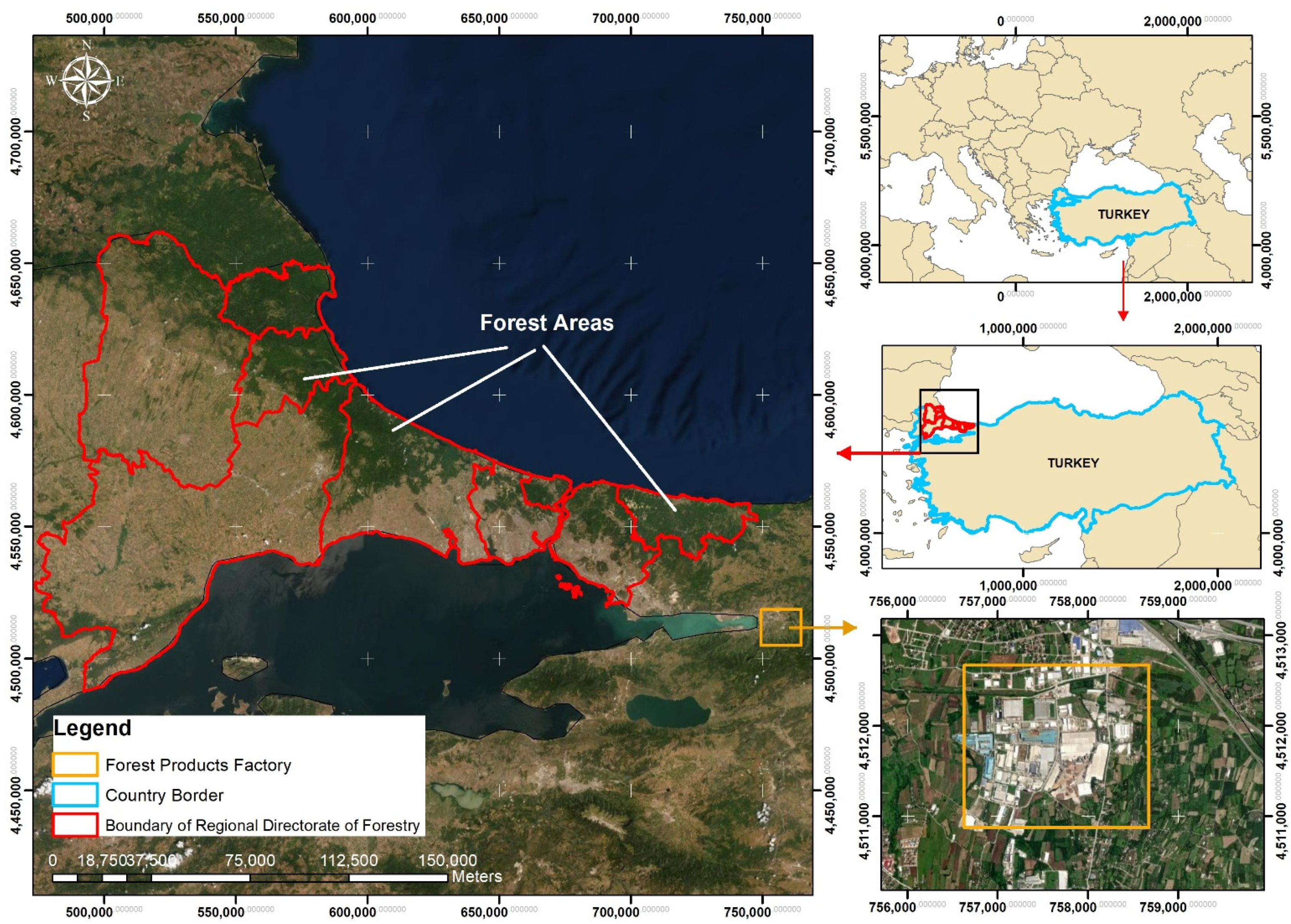
The study area includes the forest areas within the borders of forest management directorates, affiliated with the Istanbul Regional Directorate of Forestry and the forest products factory in Izmit-Kartepe in Turkey. The geographical locations of the forest areas of the Istanbul Regional Directorate of Forestry and the forest products factory are shown in Figure 1. The forest product factory has a daily production capacity of 4.200 m3 daily, producing MDF (medium density fibreload), MDFlam, laminated parquet painted plate, cover panel, lacquer panel, MDF door, door panels, and impregnated paper. In the study area, broadleaved trees are noted to produce more than coniferous trees in terms of timber harvesting amount. The total amount of timber harvested was approximately 1.3 million m3 in 2019 (Table 1).
2.2. Time Consumption Studies
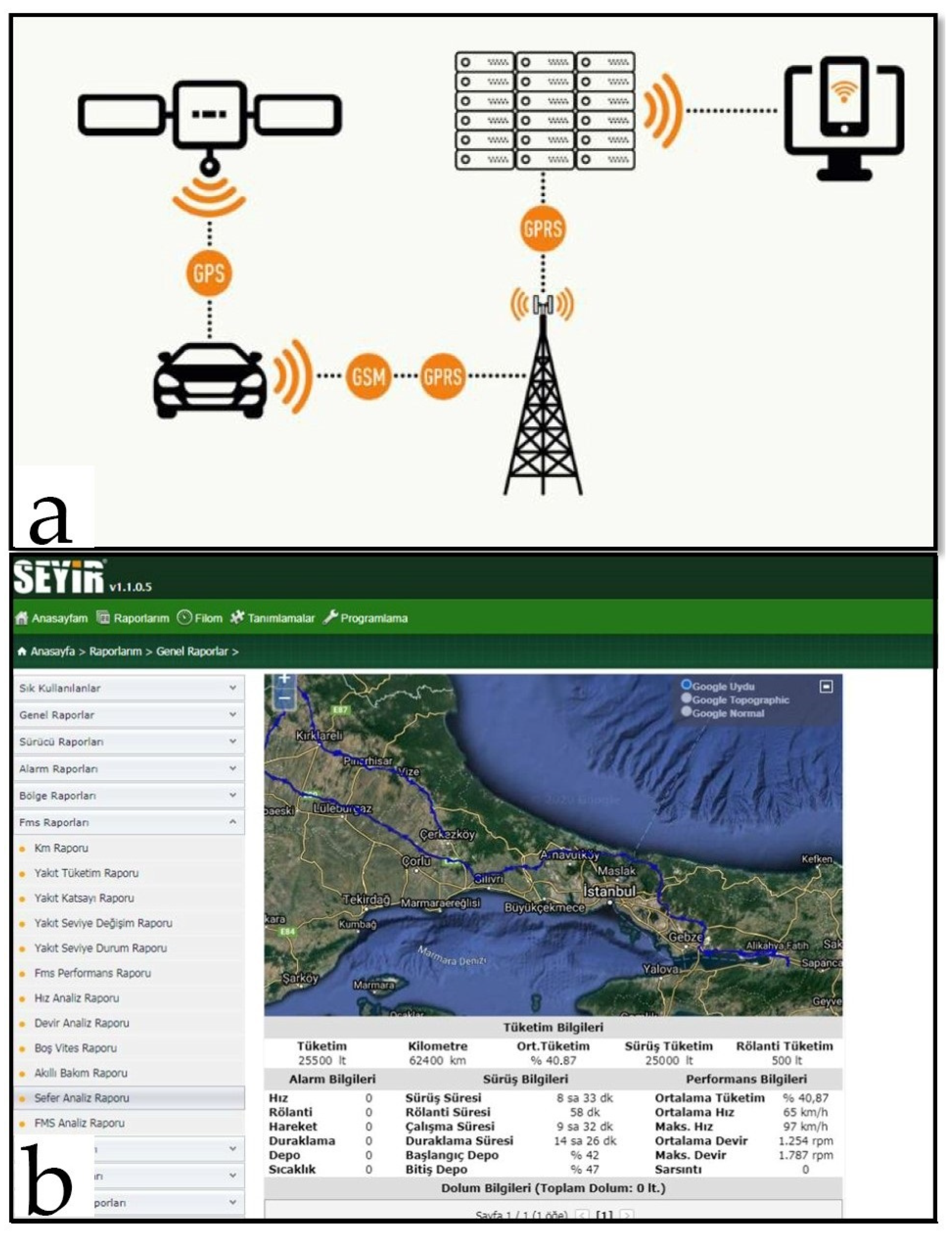
Time consumption studies were carried out to estimate the transportation vehicles’ fuel consumption values that are formed due to different conditions in the transportation of forest products. In the relevant time studies, road alignments are from the forest areas of the forest management directorates affiliated with the Istanbul Regional Directorate of Forestry to the forest products factory in Kartepe, Izmit. There are different road alignments in the study area; on average, 3 percent of each road alignment is forest road (unpaved road), and the remaining parts are asphalt and gravel roads. Sosa et al. [23] stated that classical time consumption studies are time-consuming and expensive, while fleet management systems allow automatic recording of transport activities over the long term, and there is minimal need for the driver to record. A review of relevant literature showed that geographic information system (GIS)-based vehicle tracking systems use different studies in forest products transportation [23,24,25,26,27,28,29]. Due to the disadvantages of the classical time consumption methods mentioned above, in this study, data collection regarding forest product transportation activities were carried out by means of a vehicle tracking system (Figure 2). Relevant vehicle tracking system accuracy is 2.5 m.
Five different vehicles of the five-axle semi-trailer vehicle type (legal permissible maximum load weight of 40 t) were used in the time studies related to forest products transportation. Related time studies include March, April, May, June, July and August of 2019. The transport-related data such as transport distance (km), fuel consumption (l), arrival time (minute), and maximum speed (km/h) were obtained from the vehicle tracking system website [30]. Additionally, when the relevant transport vehicles arrived at the forest products factory, they were weighed by the truck scale, and the tare weight (kg) of the transport vehicles and their total weight (kg) together with the forest product were measured. In addition, the forest product information (roundwood amount, etc.) transported by the transport vehicle and the location information where the forest product came from are also recorded by the truck scale in the forest products factory. Truck scale and forest product information were obtained from the forest products factory. After collecting the data obtained from the vehicle tracking system, the longitudinal gradient values of the road alignments where forest products are transported were calculated. Road longitudinal gradient calculations were performed as mean uphill gradient (%) and mean downhill gradient (%). Global Mapper 20 software was used to calculate the relevant road gradients. Coordinate values for road alignments were obtained from the GPS-based vehicle tracking system, which is included in the vehicles transporting forest products, using Microsoft Office Excel. The total distance of the relevant road alignments varies between 85 km and 571.2 km, with an average of 290.08 km.
In this stage, in order to calculate gradient of road alignments Shuttle Radar Topography Mission (SRTM)-based digital elevation model (DEM) data with 30 m resolution was used. At present, several DEM sources are available for users. Some of those are open source, while some of others are not free. SRTM data, which is used in the study, is one of the most commonly used open source DEM sources [31,32,33]. In addition, Mondal et al. [34] reported that SRTM (30 m) has better accuracy than other open source DEM sources SRTM (90 m), Cartosat (30 m), GTOPO (30 m), and ASTER (30 m). Then, the road alignment was obtained by combining the relevant points along the road route by the GPS in the vehicle tracking system with the “create new line feature selected points” command. In the next step, gradient analyses were made with the help of the “path profile” command. In total, the longitudinal gradients of 276 road alignments in different operational conditions (transportation distance, weight of the transport vehicle, weight of forest products, etc.) were calculated.
2.3. Fuzzy AHP Method
The analytic hierarchy process (AHP) method used in determining the weights of the criteria based on pairwise comparisons of different criteria was first proposed by Saaty [35]. The difference between the fuzzy AHP method and the AHP method is that the comparison rates are given in a range of values in the fuzzy AHP method [36]. Additionally, Zhu et al. [37] stated that the fuzzy AHP method allows the problem to be evaluated more accurately by using intermediate values instead of definite and clear values. When the relevant literature is examined, it is seen that there are different fuzzy AHP methods [38,39,40]. Van Laarhoven and Pedrycz [38] compared fuzzy ratios using triangular fuzzy numbers. Buckley [39] determined the fuzzy priorities of comparison rates by the trapezoidal membership function. In another method, Chang [40] provided a different approach by using the extent analysis method in determining triangular fuzzy numbers for pairwise comparisons. In this study, the Chang [40] extent analysis method was used. The steps for fuzzy AHP according to the extent analysis method proposed by Chang [40] are given below.
Let X = {x1, x2,...,xn} be an object test and U = {u1, u2,...,um} be a goal set. For this reason, m order analysis values are obtained for each object.
where all (j = 1, 2, … , m), whereby all are triangular fuzzy numbers.
Step 1: The fuzzy artificial size value is defined by Equation (1) with respect to the ith object.
To obtain , the fuzzy addition operation of m extent analysis values for a particular matrix is performed by using Equation (2).
Additionally, to obtain [−1, the fuzzy additional operational of (j = 1,2,..,m) values are performed as:
The inverse of the vector in Equation (3) is calculated by using Equation (4)
Step 2: The degree of possibility of M2 = (l2, u2, m2) ≥ (l1, m1, u1) is defined as follows: [Equations (5) and (6)].
where d is the ordinate of the highest intersection point D between .
Step 3: The degree possibility for a convex fuzzy number to be greater than k convex fuzzy numbers Mi (I = 1,2,…k) can be defined by Equation (7).
V (M ≥ M1 ≥ M2, …, Mi) = V [(M ≥ M1) and (M ≥ M2) and, …, and (M ≥ Mi)] = minV (M ≥ Mi)
i = 1, 2, …, k
i = 1, 2, …, k
d′(Ai) = minV(Si ≥ Sk)
Weight vector with k ≠ i for k = 1, 2,…, n is given as Equation (8)
where Ai (i = 1, 2, …, n) Ai are n elements.
W′= (d′(A1), d′(A2), …, d′(An)) T
Step 4: The weight vector normalized by the normalization process is obtained by using Equation (9)
W = (d(A1), d(A2), …, d(An)) T
2.4. TOPSIS Method
The TOPSIS method was proposed by Hwang and Yoon [41]. In the TOPSIS method, the distances to the negative ideal solution and the positive ideal solution are calculated and defined as the alternative decision option that is the furthest from the negative ideal solution and the closest to the positive ideal solution [41,42]. In the related method, a distinction between benefit and cost criteria is made [43]. The TOPSIS method consists of six stages, and the respective application steps are given below [44].
Step 1: Establish a performance matrix.
m is the number of decision points and n is the number of evaluation factors.
Step 2: Normalize the decision-matrix.
The normalized decision matrix is created by Equation (10).
The r normalized matrix is obtained as follows.
i = 1, 2, 3, m; j = 1, 2, 3, …, n
Step 3: Calculate the weighted normalized decision matrix.
By multiplying the elements in each column of the r matrix with the weights of the criteria, the V matrix is obtained.
The V matrix is shown below.
Step 4: Determine the positive ideal and negative ideal solutions.
In this step, the maximum (A*) and minimum (A−) values in each column in the weighted matrix are obtained by using Equations (11) and (12):
While j indicates the benefit function, J′ indicates the cost function.
Step 5: Calculate the separation measures. Using the Euclidean distance approach, the evaluation criteria value for each decision point has deviations from the positive ideal and negative ideal solution set. Separation measures can be obtained by using Equations (13) and (14):
Step 6: Calculate the relative closeness to ideal solution.
The relative closeness is calculated by using Equation (15):
The value obtained here is between 0 ≤≤ 1. Ci = 1 indicates that the relevant decision point is close to the positive ideal solution and Ci = 0 indicates that it is close to the negative ideal solution. The general flowchart to be used in the study is given in Figure 3.
3. Results and Discussion
3.1. Determination of Weights of Criteria by Fuzzy AHP Method
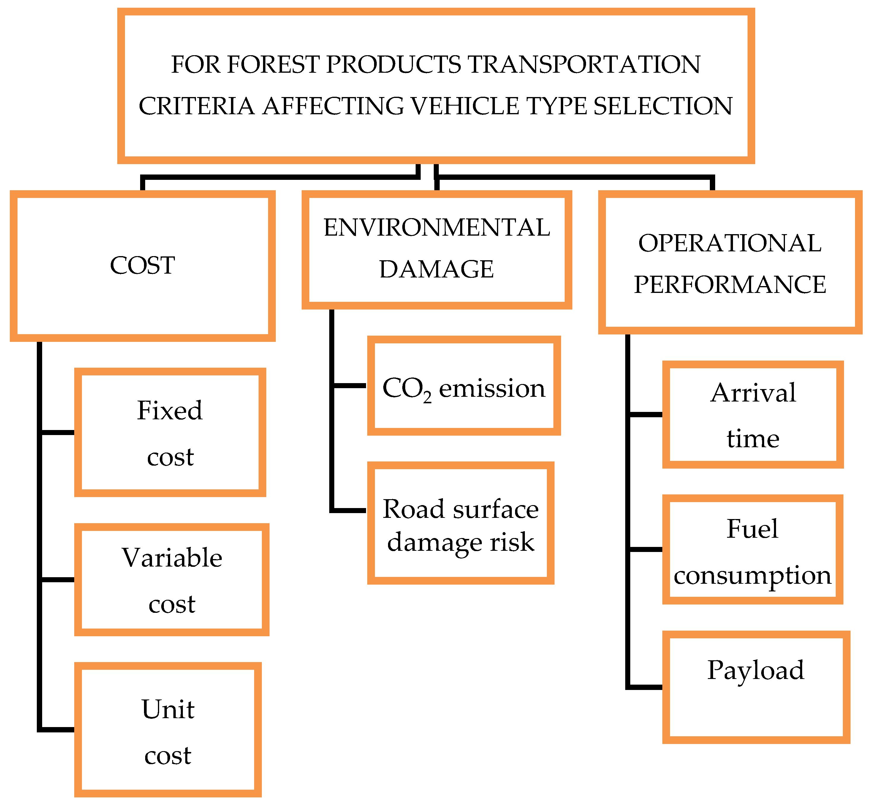
The hierarchical structure regarding the effect of criteria in determining suitable vehicle types is given in Figure 4. Cost, environmental damage, and operational performance are considered the main criteria in the determined hierarchical structure. The sub-criteria for the main cost criterion were determined to be fixed cost (depreciation, interest, insurance, and tax), variable cost (fuel, wheels, repair, and maintenance costs) and unit cost (cost per m3 of forest product transported). The sub-criteria under environmental damage were CO2 emission and risk of road surface damage (ruts, cracks, deformations, potholes, and damage to the road depending on vehicle weight). The sub-criteria under the operational performance, which is another main criterion, are arrival time (load and unload), fuel consumption (load and unload), and payload. In order to determine the weights of the criteria, a Microsoft Office Excel-based questionnaire was prepared. The relevant questionnaire form was shared with the people concerned, and their opinions were collected. In total, the opinions of 33 people (23 experts in academics, 8 in forest engineering, 2 in authorized forest products transport (person involved in logistics)) were gathered. Demographic characteristics of those who responded to the questionnaire are given in Table 2. Relevant scales used to evaluate criteria by expert persons are given in Table 3. Expert opinions are combined using the geometric mean method. After expert opinions were combined, pairwise comparison matrices were created. Calculation of the consistency ratio for the matrix for the comparison of the main criteria is given in Table 4. Before calculating the consistency ratios, the pairwise comparison matrices were defuzzification using Equation (16) [45] and the values obtained are given in Table 5.
Then, the consistency ratio was obtained by using the values of Equations (17) and (18). According to the result obtained (0.019), it can be seen that the consistency ratio of the comparison matrix is less than 0.10. The consistency rates of other pairwise comparison matrices were found to be similar. In the study, a total of four paired comparison matrices were created, one for the main criteria and three for the sub criteria. The matrix created for the main criteria, which is one of the pairwise comparison matrices, is shown in Table 4.
M = (l + 4m + u)/6
The random value index values required in the calculation of the consistency ratio is given in Table 6.
CR = Consistency ratio CI = Consistency index
RI = Random value index n = Matrix dimension λmax = Maximum eigenvalue
According to the results obtained, it was seen that the most important criterion among the main criteria was environmental damage, while the others, in order of importance, were cost and operational performance. When the sub-criteria were evaluated, it was concluded that unit cost was the most important sub-criterion of cost; of environmental damage, the most important was CO2 emission; of operational performance, it was the load capacity. Finally, the weights of the sub-criteria were multiplied by the weights of the main criteria and the general weight values were obtained (Table 7).
3.2. Prediction of Vehicle Fuel Consumption
An adaptive network-based fuzzy inference system (ANFIS) prediction model was created to calculate CO2 emissions depending on fuel consumption in different transportation scenarios. The ANFIS method was first proposed by Jang [46]. In the ANFIS method, fuzzy logic and artificial neural network methods are used together. The ANFIS method can be used in different areas because the superiority of one method overcomes the weakness of the other [47,48]. ANFIS is a method that effectively handles uncertainties encountered in any system [49]. In the fuel consumption prediction model, five inputs and one output variable were created. These variables are given in Table 8 and the description statistics are given in Table 9.
The total number of data used in the fuel consumption prediction model is 276. A randomly selected 70% of the total number of data was used in the study as training data and the remaining 30% as test data. Before analyzing the relevant data, they were transformed into (0–1) intervals by means of the minimum–maximum normalization method given in Equation (19).
x0 = Original value; Xn = Normalized value; xmin = Minimum value; xmax = Maximum value
Then, normalization values were converted to their real values with the help of Equation (20), and the values estimated by the ANFIS method were compared with the real values
In the ANFIS method, the number of iterations (epoch numbers) applied is 50 for the fuel consumption prediction model. A hybrid approach was used as the optimization method. Different membership function types and numbers have been tested for the fuel consumption prediction model. Membership function type and numbers are given in Table 10. The trapezoid membership function with the least test error was used for the fuel prediction model.
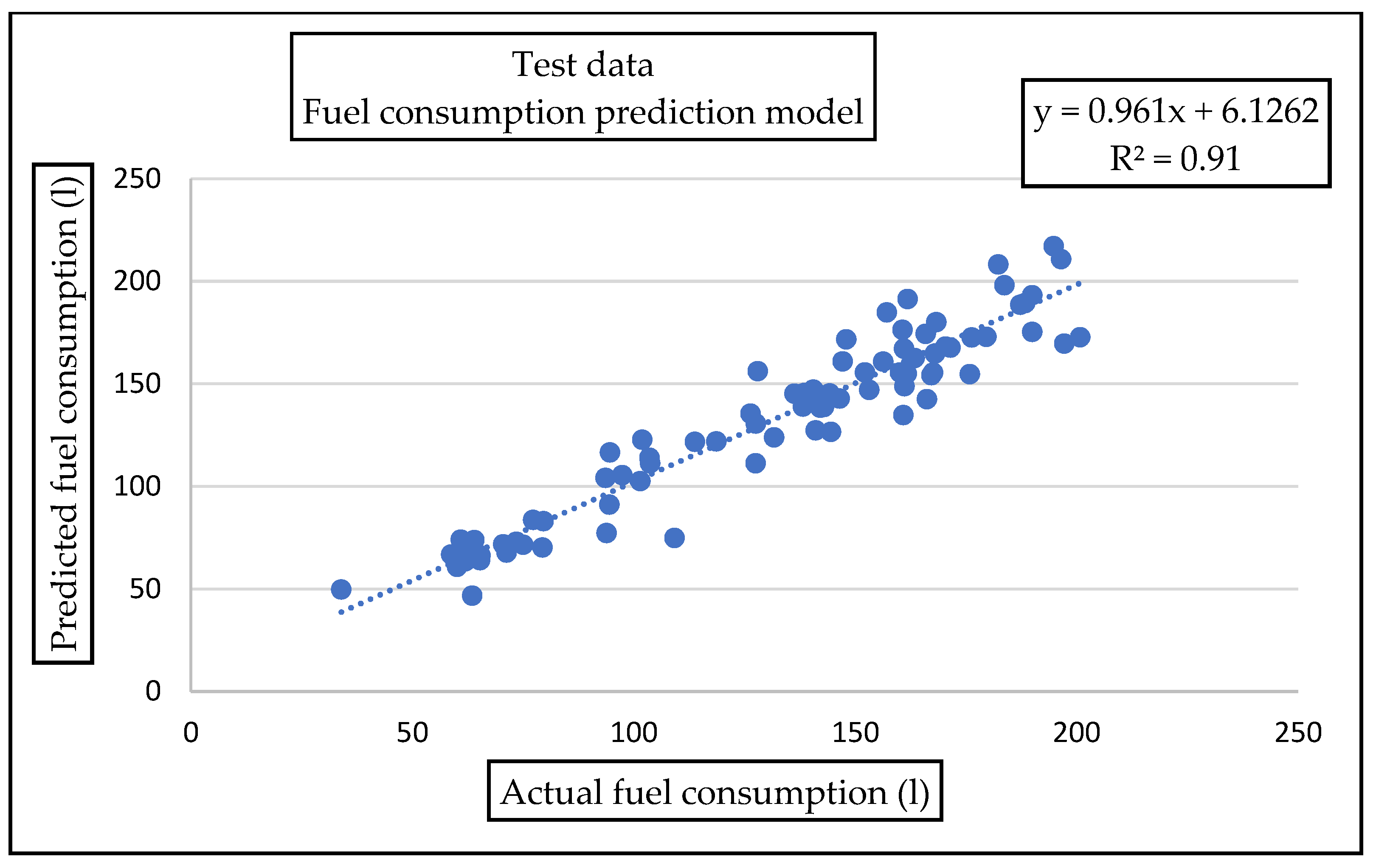
For fuel consumption prediction model, performance indicators used were “mean square error (MSE)”, “root mean squared error (RMSE)”, “mean absolute percentage error (MAPE)” and “coefficient of determination” (R2). The indicator equations are shown in Equations (21)–(24), respectively.
y1: actual output; y2: predicted output
Fuel consumption prediction model performance indicators and values are given in Table 11.
3.3. Creating Forest Product Transportation Scenarios and Determining the Most Suitable Vehicle Types in Terms of Environmental Damage
As a result of the application of the fuzzy AHP method, it was determined that the environmental damage criterion has the highest weight in terms of main criteria weight. For this reason, in the study, the most suitable vehicle types for forest product transportation under different scenarios were determined in terms of environmental damage main criteria. In the forest products transportation scenarios, the amount of forest products to be transported is divided into two groups, coniferous and broadleaved, in terms of tree group. The forest product to be transported is assumed to be logs. In determining the coniferous and broadleaved tree species, the species in the study area and the amount of wood raw material harvested were taken into account (Table 1). Accordingly, in the coniferous tree group, “Pinus nigra L.” (Black pine) and “Pinus brutia Ten.” (Red pine) were selected as tree species, while in the broadleaved tree group, “Quercus robur L./Quercus petraea L.” (Pedunculate oak/Sessile oak) and “Fagus orientalis Lipsky” (Oriental beech) were selected. Then, by using the “oven dry density” value of each tree species, the density values were obtained by using Equation (25).
where R = Density value (g/cm3), and D0 = Oven dry density (g/cm3).
Density values obtained are shown in Table 12. According to the related results, a mean of 457 kg/m3 for coniferous species and 527.5 kg/m3 for broadleaved species was calculated. Considering the moisture rates in coniferous and broadleaved tree species, density values including moisture are given in Table 13 for coniferous and broadleaved tree species. Equation (26) was used to calculate the density weights including moisture. The moisture content was noted as 35% for the coniferous tree group and 87.5% for the broadleaved tree group [50]. According to the results obtained, the broadleaved species were heavier than the coniferous ones on average (Table 12 and Table 13).
Included moisture density value = volume × density value × (1+ percent of moisture content/100)
The transportation scenarios created are given in Table 14 in terms of coniferous and broadleaved species. Forest product volumes of 50 m3, 150 m3, 200 m3, and 250 m3 were determined. Transport distances were defined as 150 km, 200 km, 250 km, and 300 km, and road longitudinal grade is determined as an uphill grade of 4% and a downhill grade of 4%. Maximum vehicle speed was defined as 90 km/h.
Vehicle alternatives were a 2-axle truck, 3-axle truck, 4-axle truck, and 5-axle semi-trailer vehicle, taking into account vehicle brands and vehicles commonly used in forest product transportation in Turkey. Maximum load weight, payload, and tare weight of these vehicles are given as mean values in Table 15 for the 2-axle truck, 3-axle truck, and 4-axle truck, while 5-axle semi-trailer vehicle maximum load weight, payload, and tare weight values are given as mean values in Table 16.
Fuel consumption values of vehicle alternatives were calculated using an ANFIS-based prediction model. CO2 emission values based on fuel consumption values of transport vehicles were calculated based on the TIER I approach proposed by the Intergovernmental Panel on Climate Change (IPCC). The TIER I approach was developed to predict CO2 emission and other greenhouse gas emissions to a certain extent in cases where detailed data on issues such as vehicle parking, operating conditions, fuel consumption, emission factors, and technology level of vehicles are not available. It is a method applied according to the principle of calculating the emission that will arise in proportion to how much fuel is used in a country [51] The TIER I approach to the CO2 emission calculation method is given in Equation (27). Diesel fuel was used in the calculation of CO2 emission.
E = Emission of CO2 (kg); Fuela = Fuel sold (TJ)
EFa = Emission factor (kg/TJ)—carbon content of the fuel multiplied by 44/12
a = Type of fuel
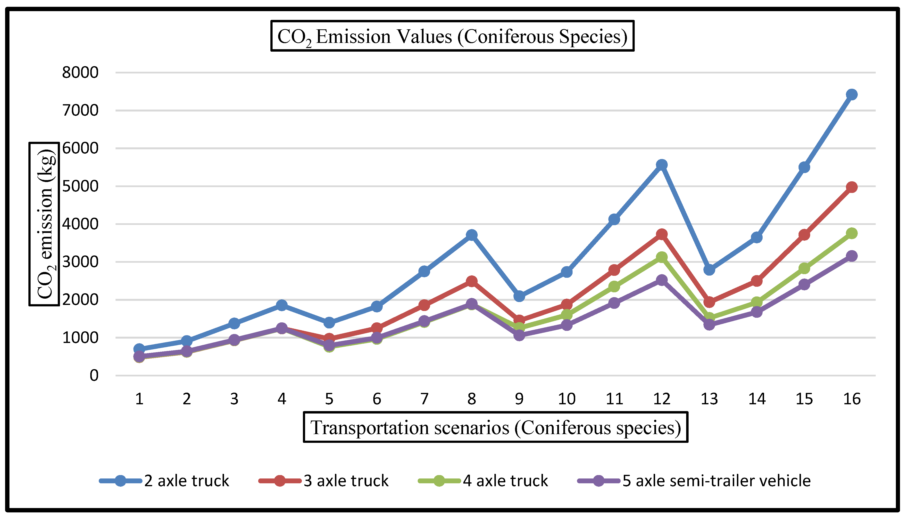
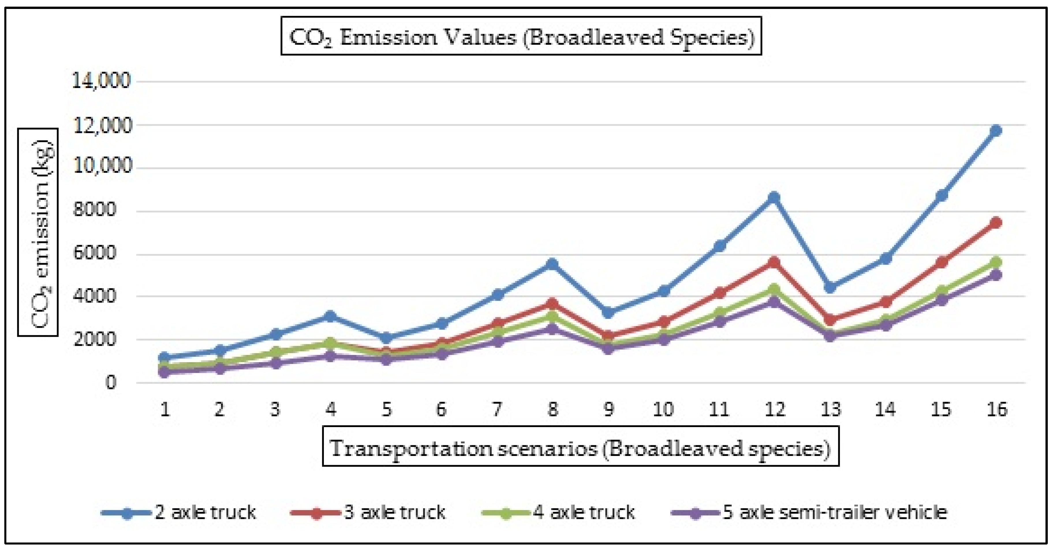
The estimated fuel consumption values for the transportation scenarios created for coniferous species and broadleaved species and the CO2 emission values formed depending on the fuel consumption values are given in Table 17 and Table 18 and in Figure 7 and Figure 8. In the transportation scenarios created for coniferous species, it has been observed that the vehicle type with the highest CO2 emission is the 2-axle truck. When all transportation scenarios are evaluated, the vehicle type with the lowest CO2 emission is generally a 5-axle semi-trailer vehicle. In the first four transport scenarios created for broadleaved species, the CO2 emission of the 5-axle semi-trailer vehicle is generally lower than the other vehicle types, followed by the 3-axle truck and 4-axle truck with similar values, and the highest CO2 emission is from the 2-axle truck. In other transportation scenarios, emissions values in descending order are for 2-axle trucks, 3-axle trucks, 4-axle trucks, and 5-axle semi-trailers.
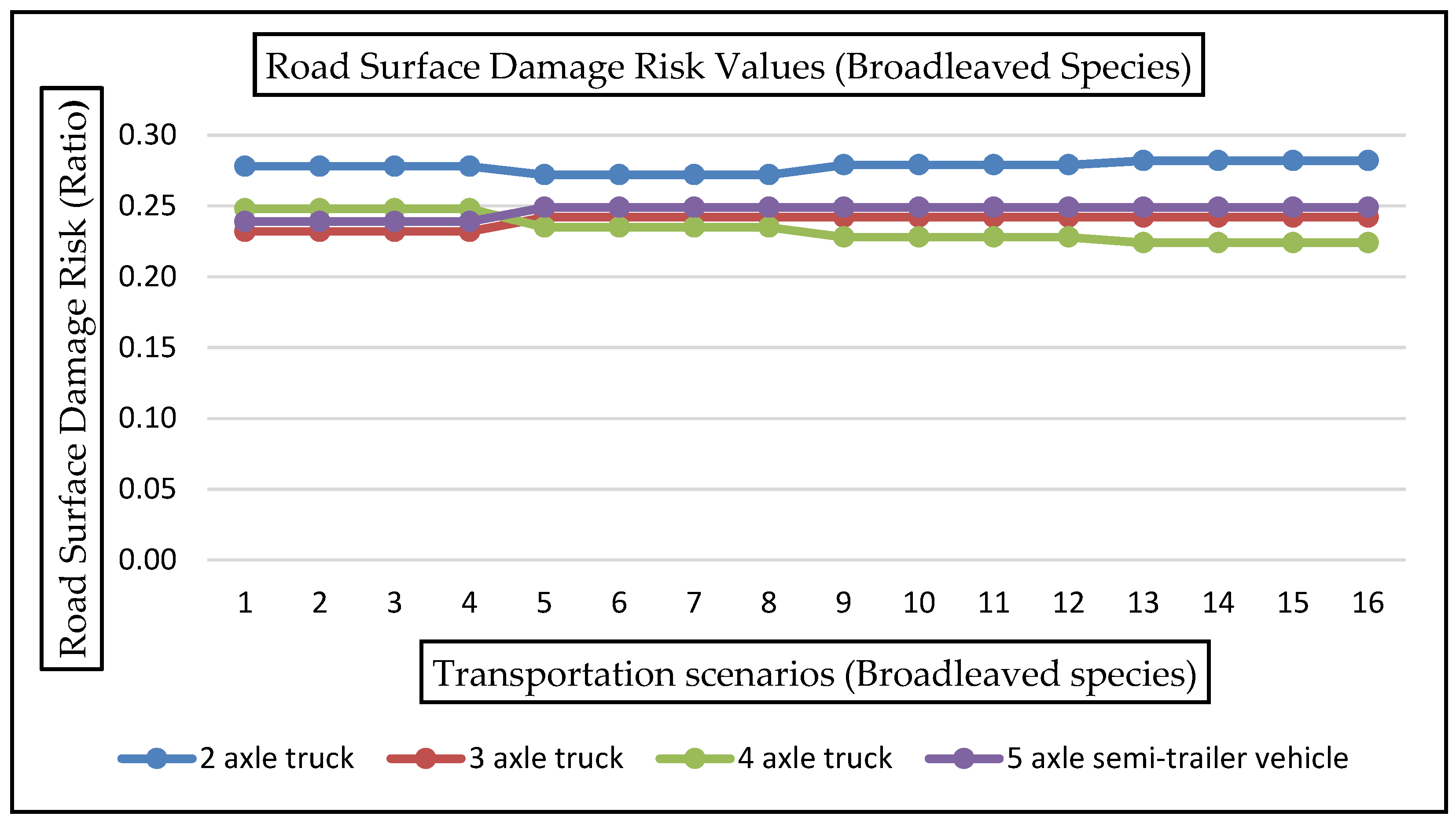
On the other hand, the risk of damage to the road surface (ruts, cracks, deformations, potholes, etc.) depends on the transportation vehicles tare weight and gross weight. Road surface damage risk is obtained as a ratio. For example, in the transportation scenarios created for coniferous tree species, obtaining the road surface damage risk of a 2-axle vehicle for the first transportation scenario is given in Equation (28).
Road surface damage risk values are given in Table 19 and Table 20 and in Figure 9 and Figure 10 for coniferous species and broadleaved species. When the transportation scenarios for road surface damage risks for coniferous species are evaluated, the risk values of vehicle types differ according to the transportation scenario. When the road surface damage risk values are analyzed for broadleaved, the highest risk of damage in all transportation scenarios is the 2-axle truck. When other vehicle types are evaluated, it is determined that the vehicle with the lowest risk of road surface damage in the first four scenarios is a 3-axle truck, whereas in other transportation scenarios it is a 4-axle truck.
3.4. Results for Determining the Most Suitable Vehicle Types in Transportation Scenarios
In order to determine the rank of suitable vehicle alternatives in terms of environmental damage, a hybrid fuzzy multi-criteria decision-making method was used in the transportation scenarios. First, relevant criteria weight values were calculated using the fuzzy AHP method. Next, the rank of suitable vehicle alternatives was determined using the TOPSIS method. In this context, for the TOPSIS method application, relevant criteria were taken into consideration, such as cost.
For example, in terms of coniferous tree species, the vehicle type suitability rankings for the first transport scenario are shown below. First, a standard decision matrix was created for the application of the TOPSIS method; this is given in Table 21. Next, the decision matrix was normalized and weighted using the weight values of the related to sub-criteria for the fuzzy AHP method (Table 21). Then, the positive ideal solution (PIS) and the negative ideal solution (NIS) were found, and the alternatives are listed (Table 21 and Table 22).
Considering the transportation scenarios for coniferous tree species, it is seen that in the scenario created for 50 m3 forest product to be transported, a 3-axle truck is the most suitable vehicle type for all transportation distances, followed by a 4-axle truck, 5-axle semi-trailer vehicle, and 2-axle truck. In the transportation scenario for 100 m3 of forest product to be transported, the most suitable vehicle type is a 4-axle truck at all transport distances, followed by 5-axle semi-trailer vehicle, 3-axle truck, and a 2-axle truck. For all transportation scenarios of 150 m3 and 200 m3, the most suitable vehicle type is a 5-axle semi-trailer vehicle, while other suitable vehicle types are 4-axle trucks, 3-axle trucks, and 2-axle trucks (Table 23).
When the transportation of broadleaved tree species is evaluated in terms of environmental damage, it is seen that the most suitable vehicle type for all transportation distances of the scenario created for 50 m3 of forest product is a 5-axle semi-trailer vehicle, 3-axle truck, 4-axle truck, and 2-axle truck. For 100 m3 of forest product, the ranking of suitable vehicle types at all transport distances is the 5-axle semi-trailer vehicle, 4-axle truck, 3-axle truck, and 2-axle truck. For 150 m3 of forest product, the ranking of suitable vehicle types at 150 km transport distance is the 4-axle truck, 5-axle semi-trailer vehicle, 3-axle truck, and 2-axle truck. In other transportation distances, the order was a 5-axle semi-trailer vehicle, 4-axle truck, 3-axle truck, and 2-axle truck. Finally, when the amount of forest products to be transported was evaluated at 200 m3, it was concluded that the ranking of suitable vehicle types is the 4-axle truck, 5-axle semi-trailer vehicle, 3-axle truck, and 2-axle truck at all transportation distances (Table 24).
In the vehicle type suitability rankings, which take into account the CO2 emission and road surface damage risk, some differences were determined in terms of coniferous and broadleaved tree groups. In terms of coniferous tree species, it was concluded that the most suitable vehicle type for transporting 50 m3 and 100 m3 of forest products is a 3-axle truck and a 4-axle truck, and in other transportation scenarios, the most suitable vehicle type is a 5-axle semi-trailer vehicle. The coniferous species are less dense compared to broadleaved species, so especially in cases where less product is transported, a vehicle with less load capacity compared to a 5-axle semi-trailer vehicle creates a lower total truck weight (gross and tare). As a result, it is possible to achieve less road surface damage and less CO2 emission due to fuel consumption. Sosa et al. [4] reported that there is a strong function between axle load and pavement, and small increases in load increase major pavement damage. In a similar study, Palander [52] compared trucks with a maximum loaded weight of 64 t, 68 t, 76 t and 92 t in terms of environmental and energy efficiency in wood transport, and stated that the energy efficiency of 64 t and 68 t trucks with small loads is better than other vehicles.
In the transportation scenarios regarding the broadleaved tree species, in general, it is seen that the most suitable vehicle type is a 5-axle semi-trailer vehicle. Tymendorf and Trzciński [53] stated that the density and moisture content of wood significantly affect the weight of the load. Sosa et al. [54], on the other hand, stated that the moisture content affects the efficiency of the truck and reduces the total amount of transported product. Murphy et al. [55] stated that the decrease in the amount of water in the wood results in less water per load. In this context, it is thought that this may be due to the increase in the number of vehicles required, as the broadleaved tree group is heavier in volume (density) than the coniferous tree group and contains more moisture. Klvač et al. [56] stated that fuel consumption by trucks increases greenhouse gas emissions that cause environmental pollution. Consistent with these results, Liimatainen et al. [57] and Palender [58] stated that increasing the maximum allowable truck load weights leads to a decrease in CO2 emissions. Busenius et al. [59] stated that if the maximum permissible weight for vehicles were increased from 40 tons to 44 tons, greenhouse gas emissions would decrease by 13%. Kanzian et al. [60] concluded that a decrease in moisture content from 40% to 30% reduces greenhouse gas emissions into the atmosphere.
4. Conclusions
In this study, the suitability of vehicle alternatives in forest product transportation was determined effectively by the weight values of the criteria. In addition, taking into account the weight values of the sub-criteria in the environmental damage main criteria, a scenario-based analysis was carried out, and the vehicle type suitability ranks were revealed in terms of coniferous and broadleaved tree species. According to the results obtained, there is a difference in vehicle type suitability rankings in forest products transportation scenarios in terms of coniferous and broadleaved tree species. Consequently, it is thought that considering the amount of forest products to be transported and the tree species will be beneficial for transportation planning. In relation to this, the tree species in the study area should be evaluated in terms of density values and the amount of moisture content that may vary depending on seasonal conditions, and planning should be performed accordingly. This is important in terms of preventing exceeding the maximum legally allowed vehicle load weights. In addition, considering environmental damage, less CO2 emission and less road surface damage risk will be achieved. The results obtained in future studies by considering different evaluation criteria and using different multi-criteria decision-making methods can be compared with the results of this study. In this study, vehicle type alternatives were determined in terms of those vehicle brands and types commonly used in forest product transportation. For this reason, vehicle alternatives can be diversified by considering the objectives of the forest management directorate, the operational possibilities at hand, the dimensions of the forest products to be transported (forest product diameter–length values, etc.), the existing road conditions, and the timber harvesting methods used. In addition, different transportation scenarios can be created by considering seasonal conditions and different road alignments. In this way, vehicle alternatives in terms of environmental damage risk can be revealed in more detail, and the conformity of vehicle alternatives can be obtained more effectively according to the relevant transportation scenarios to be created.
Author Contributions
Conceptualization, methodology, investigation, A.O.A. and M.D.; data collection and analysis, A.O.A. and M.D.; writing and editing, A.O.A. and M.D. All authors have read and agreed to the published version of the manuscript.
Funding
This research received no external funding.
Data Availability Statement
The data presented in this study are available on request from the corresponding author.
Acknowledgments
This study partly contains some results presented in the thesis of Anil Orhan Akay in Advisory of Murat Demir completed in 2021 at Istanbul University-Cerrahpaşa Institute of Graduate Studies. We would like to thank the expert academicians, forest engineers and forest products transportation authorities for contributing to this study by responding to the questionnaire prepared to assess the relevant criteria.
Conflicts of Interest
The authors declare no conflict of interest.
References
- El Hachemi, N.; Gendreau, M.; Rousseau, L.-M. Solving a Log-Truck Scheduling Problem with Constraint Programming. In Proceedings of the International Conference on Integration of Artificial Intelligence (AI) and Operations Research (OR) Techniques in Constraint Programming, Paris, France, 20–23 May 2008; Springer: Berlin/Heidelberg, Germany; pp. 293–297. [Google Scholar]
- Koirala, A.; Kizha, A.R.; Roth, B. Forest Trucking Industry in Maine: A Review on Challenges and Resolutions. In Proceedings of the 39th Annual Meeting of the Council on Forest Engineering, Vancouver, BC, Canada, 19–21 September 2016. [Google Scholar]
- Nurminen, T.; Heinonen, J. Characteristics and Time Consumption of Timber Trucking in Finland. Silva Fenn. 2007, 41, 471–487. [Google Scholar] [CrossRef] [Green Version]
- Sosa, A.; Klvac, R.; Coates, E.; Kent, T.; Devlin, G. Improving Log Loading Efficiency for Improved Sustainable Transport within the Irish Forest and Biomass Sectors. Sustainability 2015, 7, 3017–3030. [Google Scholar] [CrossRef] [Green Version]
- OECD. Biomass and Agriculture: Sustainability, Markets and Policies; Organisation for Economic Co-operation and Development: Paris, France, 2004. [Google Scholar]
- Weintraub, A.; Romero, C.; Bjørndal, T.; Epstein, R.; Miranda, J. Handbook of Operations Research in Natural Resources; Springer Science & Business Media: Berlin/Heidelberg, Germany, 2007. [Google Scholar]
- Devlin, G.; Sosa, A.; Acuna, M. Solving the Woody Supply Chain for Ireland’s Expanding Biomass Sector: A Case Study. In Biomass Supply Chains for Bioenergy and Biorefining; Elsevier: Amsterdam, The Netherlands, 2016; pp. 333–355. [Google Scholar]
- Hamsley, A.K.; Greene, W.D.; Siry, J.P.; Mendell, B.C. Improving Timber Trucking Performance by Reducing Variability of Log Truck Weights. South. J. Appl. For. 2007, 31, 12–16. [Google Scholar] [CrossRef] [Green Version]
- Mousavi, R. Comparison of Productivity, Cost and Environmental Impacts of Two Harvesting Methods in Northern Iran: Short-Log vs. Long-Log. Ph.D. Thesis, Faculty of Forest Sciences, University of Joensuu, Joensuu, Finland, 2009. [Google Scholar]
- Rönnqvist, M.; D’Amours, S.; Weintraub, A.; Jofre, A.; Gunn, E.; Haight, R.G.; Martell, D.; Murray, A.T.; Romero, C. Operations Research Challenges in Forestry: 33 Open Problems. Ann. Oper. Res. 2015, 232, 11–40. [Google Scholar] [CrossRef]
- Lautala, P.T.; Hilliard, M.R.; Webb, E.; Busch, I.; Hess, J.R.; Roni, M.S.; Hilbert, J.; Handler, R.M.; Bittencourt, R.; Valente, A. Opportunities and Challenges in the Design and Analysis of Biomass Supply Chains. Environ. Manag. 2015, 56, 1397–1415. [Google Scholar] [CrossRef]
- Svenson, G.; Fjeld, D. The Impact of Road Geometry and Surface Roughness on Fuel Consumption of Logging Trucks. Scand. J. For. Res. 2016, 31, 526–536. [Google Scholar] [CrossRef]
- Han, S.-K.; Murphy, G. Predicting Loaded On-Highway Travel Times of Trucks Hauling Woody Raw Material for Improved Forest Biomass Utilization in Oregon. West. J. Appl. For. 2012, 27, 92–99. [Google Scholar] [CrossRef]
- Mousavi, R.; Naghdi, R. Time Consumption and Productivity Analysis of Timber Trucking Using Two Kinds of Trucks in Northern Iran. J. For. Sci. 2013, 59, 211–221. [Google Scholar] [CrossRef] [Green Version]
- Manzone, M.; Balsari, P. The Energy Consumption and Economic Costs of Different Vehicles Used in Transporting Woodchips. Fuel 2015, 139, 511–515. [Google Scholar] [CrossRef]
- Manzone, M.; Calvo, A. Woodchip Transportation: Climatic and Congestion Influence on Productivity, Energy and CO2 Emission of Agricultural and Industrial Convoys. Renew. Energy 2017, 108, 250–259. [Google Scholar] [CrossRef]
- Trzciński, G.; Moskalik, T.; Wojtan, R. Total Weight and Axle Loads of Truck Units in the Transport of Timber Depending on the Timber Cargo. Forests 2018, 9, 164. [Google Scholar] [CrossRef] [Green Version]
- Achillas, C.; Moussiopoulos, N.; Karagiannidis, A.; Banias, G.; Perkoulidis, G. The Use of Multi-Criteria Decision Analysis to Tackle Waste Management Problems: A Literature Review. Waste Manag. Res. 2013, 31, 115–129. [Google Scholar] [CrossRef] [PubMed]
- Akay, A.O.; Demir, M.; Akgul, M. Assessment of Risk Factors in Forest Road Design and Construction Activities with Fuzzy Analytic Hierarchy Process Approach in Turkey. Environ. Monit. Assess. 2018, 190, 1–12. [Google Scholar] [CrossRef] [PubMed]
- Saremi, M.; Mousavi, S.F.; Sanayei, A. TQM Consultant Selection in SMEs with TOPSIS under Fuzzy Environment. Expert Syst. Appl. 2009, 36, 2742–2749. [Google Scholar] [CrossRef]
- Karakasoglu, N. Fuzzy Multi-Criteria Decision Making Methods and Application. Master’s Thesis, Pamukkale University Graduate School of Social Sciences, Denizli, Turkey, 2008. (In Turkish). [Google Scholar]
- GDF General Directorate of Forestry Istanbul Regional Directorate of Forestry Wood Raw Material Harvesting Amounts. Available online: https://www.ogm.gov.tr/ekutuphane/UretimSatisveStokFaaliyetleri/Forms/AllItems.aspx (accessed on 30 October 2020).
- Sosa, A.; McDonnell, K.; Devlin, G. Analysing Performance Characteristics of Biomass Haulage in Ireland for Bioenergy Markets with GPS, GIS and Fuel Diagnostic Tools. Energies 2015, 8, 12004–12019. [Google Scholar] [CrossRef]
- Sikanen, L.; Asikainen, A.; Lehikoinen, M. Transport Control of Forest Fuels by Fleet Manager, Mobile Terminals and GPS. Biomass Bioenergy 2005, 28, 183–191. [Google Scholar] [CrossRef]
- Devlin, G.J.; McDonnell, K.; Ward, S. Timber Haulage Routing in Ireland: An Analysis Using GIS and GPS. J. Transp. Geogr. 2008, 16, 63–72. [Google Scholar] [CrossRef] [Green Version]
- Holzleitner, F.; Kanzian, C.; Stampfer, K. Analyzing Time and Fuel Consumption in Road Transport of Round Wood with an Onboard Fleet Manager. Eur. J. For. Res. 2011, 130, 293–301. [Google Scholar] [CrossRef]
- Conrad, I.; Joseph, L. Would Weight Parity on Interstate Highways Improve Safety and Efficiency of Timber Transportation in the US South? Int. J. For. Eng. 2020, 31, 242–252. [Google Scholar] [CrossRef]
- Conrad, J.L. Evaluating Profitability of Individual Timber Deliveries in the US South. Forests 2021, 12, 437. [Google Scholar] [CrossRef]
- Pandur, Z.; Nevečerel, H.; Šušnjar, M.; Bačić, M.; Lepoglavec, K. Energy Efficiency of Timber Transport by Trucks on Hilly and Mountainous Forest Roads. Forestist 2022, 72, 20–28. [Google Scholar] [CrossRef]
- Seyir Vehicle Tracking and Fleet Management System. Available online: http://web.seyirmobil.com/ (accessed on 10 July 2019).
- Boulton, S.J.; Stokes, M. Which DEM Is Best for Analyzing Fluvial Landscape Development in Mountainous Terrains? Geomorphology 2018, 310, 168–187. [Google Scholar] [CrossRef]
- Esin, A.İ.; Akgul, M.; Akay, A.O.; Yurtseven, H. Comparison of LiDAR-Based Morphometric Analysis of a Drainage Basin with Results Obtained from UAV, TOPO, ASTER and SRTM-Based DEMs. Arab. J. Geosci. 2021, 14, 340. [Google Scholar] [CrossRef]
- Gülci, S.; Akgül, M.; Gülci, N.; Demir, M. Orman Yolu Güzergahlarının Belirlenmesinde Farklı Tekniklerle Üretilmiş Sayısal Arazi Modellerinin Kullanılması Üzerine Bir Araştırma (A Study on Using Digital Terrain Models Produced by Different Techniques in Determining Forest Road Routes). J. Bartin Fac. For. 2021, 23, 654–667. (In Turkish) [Google Scholar] [CrossRef]
- Mondal, A.; Khare, D.; Kundu, S. Uncertainty Analysis of Soil Erosion Modelling Using Different Resolution of Open-Source DEMs. Geocarto Int. 2017, 32, 334–349. [Google Scholar] [CrossRef]
- Saaty, T.L. The Analytic Hierarchy Process Mcgraw Hill, New York. Agric. Econ. Rev. 1980, 70, 324. [Google Scholar]
- Bender, M.J.; Simonovic, S.P. A Fuzzy Compromise Approach to Water Resource Systems Planning under Uncertainty. Fuzzy Sets Syst. 2000, 115, 35–44. [Google Scholar] [CrossRef]
- Zhu, K.-J.; Jing, Y.; Chang, D.-Y. A Discussion on Extent Analysis Method and Applications of Fuzzy AHP. Eur. J. Oper. Res. 1999, 116, 450–456. [Google Scholar] [CrossRef]
- Van Laarhoven, P.J.; Pedrycz, W. A Fuzzy Extension of Saaty’s Priority Theory. Fuzzy Sets Syst. 1983, 11, 229–241. [Google Scholar] [CrossRef]
- Buckley, J.J. Fuzzy Hierarchical Analysis. Fuzzy Sets Syst. 1985, 17, 233–247. [Google Scholar] [CrossRef]
- Chang, D.-Y. Applications of the Extent Analysis Method on Fuzzy AHP. Eur. J. Oper. Res. 1996, 95, 649–655. [Google Scholar] [CrossRef]
- Hwang, C.-L.; Yoon, K. Methods for Multiple Attribute Decision Making. In Multiple Attribute Decision Making; Springer: Berlin/Heidelberg, Germany, 1981; pp. 58–191. [Google Scholar]
- Cheng, S.; Chan, C.W.; Huang, G.H. Using Multiple Criteria Decision Analysis for Supporting Decisions of Solid Waste Management. J. Environ. Sci. Health Part A 2002, 37, 975–990. [Google Scholar] [CrossRef] [PubMed]
- Janic, M. Multicriteria Evaluation of High-Speed Rail, Transrapid Maglev and Air Passenger Transport in Europe. Transp. Plan. Technol. 2003, 26, 491–512. [Google Scholar] [CrossRef]
- Jahanshahloo, G.R.; Lotfi, F.H.; Izadikhah, M. An Algorithmic Method to Extend TOPSIS for Decision-Making Problems with Interval Data. Appl. Math. Comput. 2006, 175, 1375–1384. [Google Scholar] [CrossRef]
- Kwong, C.-K.; Bai, H. Determining the Importance Weights for the Customer Requirements in QFD Using a Fuzzy AHP with an Extent Analysis Approach. IIE Trans. 2003, 35, 619–626. [Google Scholar] [CrossRef]
- Jang, J.-S. ANFIS: Adaptive-Network-Based Fuzzy Inference System. IEEE Trans. Syst. Man Cybern. 1993, 23, 665–685. [Google Scholar] [CrossRef]
- Jang, J.-S.R.; Sun, C.-T.; Mizutani, E. Neuro-Fuzzy and Soft Computing-a Computational Approach to Learning and Machine Intelligence [Book Review]. IEEE Trans. Autom. Control 1997, 42, 1482–1484. [Google Scholar] [CrossRef]
- Kim, J.; Kasabov, N. HyFIS: Adaptive Neuro-Fuzzy Inference Systems and Their Application to Nonlinear Dynamical Systems. Neural Netw. 1999, 12, 1301–1319. [Google Scholar] [CrossRef]
- Saravanan, S.; Kannan, S.; Thangaraj, C. Prediction of India’s Electricity Demand Using Anfis. ICTACT J. Soft Comput. 2015, 5, 985–990. [Google Scholar]
- Bozkurt, A.Y.; Erdin, N. Ağaç Malzeme Teknolojisi (Wood Technology); Istanbul University Press: Istanbul, Turkey, 2011. (In Turkish) [Google Scholar]
- Houghton, J.T.; Meira Filho, L.G.; Lim, B.; Treanton, K.; Mamaty, I.; Bonduki, Y.; Griggs, D.J.; Callender, B.A. (Eds.) IPCC/UNEP/OECD/IEA Revised 1996 IPCC Guidelines for National Greenhouse Gas Inventories Volume III: Reference Manual; Intergovernmental Panel on Climate Change, United Nations Environment Programme, Organization for Economic CoOperation and Development, International Energy Agency: Paris, France, 1997; Chapter 1; pp. 4–44, 62–98. [Google Scholar]
- Palander, T.; Haavikko, H.; Kortelainen, E.; Kärhä, K.; Borz, S.A. Improving Environmental and Energy Efficiency in Wood Transportation for a Carbon-Neutral Forest Industry. Forests 2020, 11, 1194. [Google Scholar] [CrossRef]
- Tymendorf, L.; Trzciński, G. Multi-Factorial Load Analysis of Pine Sawlogs in Transport to Sawmill. Forests 2020, 11, 366. [Google Scholar] [CrossRef] [Green Version]
- Sosa, A.; Acuna, M.; McDonnell, K.; Devlin, G. Controlling Moisture Content and Truck Configurations to Model and Optimise Biomass Supply Chain Logistics in Ireland. Appl. Energy 2015, 137, 338–351. [Google Scholar] [CrossRef] [Green Version]
- Murphy, G.; Kent, T.; Kofman, P.D. Modeling Air Drying of Sitka Spruce (Picea Sitchensis) Biomass in off-Forest Storage Yards in Ireland. For. Prod. J. 2012, 62, 443–449. [Google Scholar] [CrossRef]
- Klvač, R.; Kolařík, J.; Volná, M.; Drápela, K. Fuel Consumption in Timber Haulage. Croat. J. For. Eng. J. Theory Appl. For. Eng. 2013, 34, 229–240. [Google Scholar]
- Liimatainen, H.; Pöllänen, M.; Nykänen, L. Impacts of Increasing Maximum Truck Weight—Case Finland. Eur. Transp. Res. Rev. 2020, 12, 14. [Google Scholar] [CrossRef] [Green Version]
- Palander, T. The Environmental Emission Efficiency of Larger and Heavier Vehicles—A Case Study of Road Transportation in Finnish Forest Industry. J. Clean. Prod. 2017, 155, 57–62. [Google Scholar] [CrossRef]
- Busenius, M.; Engler, B.; Smaltschinski, T.; Opferkuch, M. Consequences of Increasing Payloads on Carbon Emissions–an Example from the Bavaria State Forest Enterprise (BaySF). For. Lett. 2015, 108, 7–14. [Google Scholar]
- Kanzian, C.; Kühmaier, M.; Erber, G. Effects of Moisture Content on Supply Costs and CO2 Emissions for an Optimized Energy Wood Supply Network. Croat. J. For. Eng. J. Theory Appl. For. Eng. 2016, 37, 51–60. [Google Scholar]
Figure 1.
Study area location.

Figure 2.
Vehicle tracking system general view (a) and vehicle tracking system web-based report view (b).
Figure 2.
Vehicle tracking system general view (a) and vehicle tracking system web-based report view (b).

Figure 3.
The flowchart of proposed for hybrid fuzzy multi criteria decision system.

Figure 4.
Hierarchical structure of main criteria and sub-criteria for vehicle type selection.

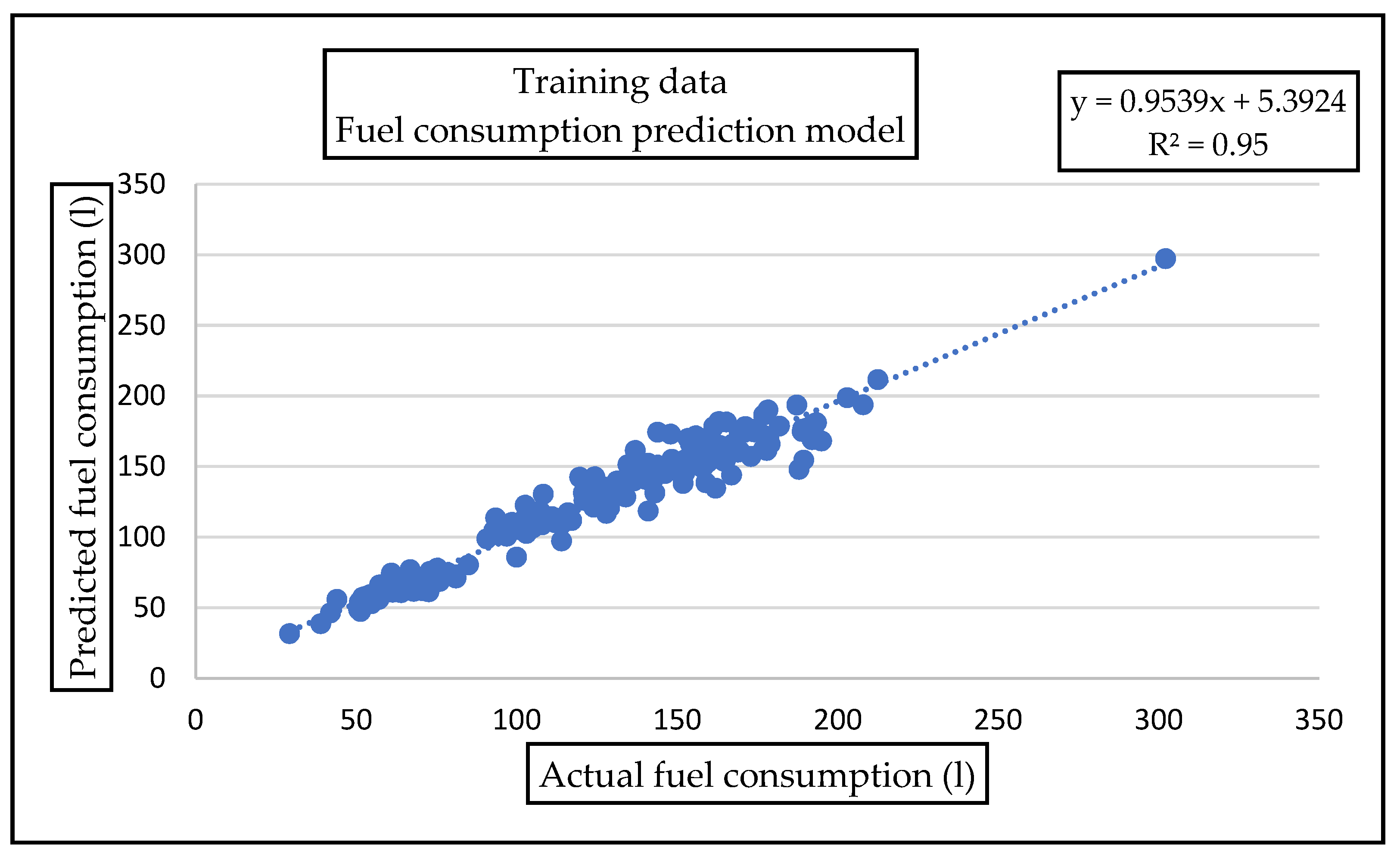
Figure 5.
R2 values of actual and predicted fuel consumption for training data using ANFIS.

Figure 6.
R2 values of actual and predicted fuel consumption for test data using ANFIS.

Figure 7.
CO2 emission values for coniferous species in terms of transportation scenarios.

Figure 8.
CO2 emission values for broadleaved species in terms of transportation scenarios.

Figure 9.
Road surface risk values for coniferous species.

Figure 10.
Road surface risk values for broadleaved species.


Table 1.
Timber harvesting values in study area [22].
Table 1.
Timber harvesting values in study area [22].
| Coniferous Tree Group | Timber Harvesting (m3) | Broadleaved Tree Group | Timber Harvesting (m3) |
|---|---|---|---|
| Cedrussp. (Cedar) | 0 | Quercussp. (Oak) | 578,931 |
| Juniperus(Juniper) | 0 | Carpinussp.(Hornbeam) | 12,600 |
| Pinus brutiaTen. (Red pine) | 30,572 | Fagussp.(Beech) | 318,674 |
| Pinus sylvestrisL. (Scotch pine) | 109 | Populussp.(Poplar) | 10,296 |
| Pinus nigraL. (Black pine) | 81,181 | Alnussp.(Alder) | 1453 |
| Piceasp. (Spruce) | 0 | Other broadleaved | 81,926 |
| Abiessp. (Fir) | 0 | Total (broadleaved) | 1,003,880 |
| Other coniferous | 161,975 | ||
| Total (coniferous) | 273,837 | ||
| General total (m3) (coniferous + broadleaved) | 1,277,717 | ||
Table 2.
Demographic characteristics of the persons participating in the questionnaire.
| Demographic Characteristics | Occupational Status of the Surveyor Evaluators | |||||
|---|---|---|---|---|---|---|
| Expert academicians (22 male; 1 female) | Forest engineer (6 male; 2 female) | Forest products transportation authorized (Persons involved in logistics) (2 male) | ||||
| Age | 20–40 | 11 persons | 30–40 | 2 persons | 30–40 | 2 persons |
| 40–60 | 11 persons | 40–50 | 6 persons | |||
| >60 | 1 person | |||||
| Occupational experience (year) | 3–10 | 6 persons | 0–10 | 2 persons | 10–15 | 2 persons |
| 10–20 | 10 persons | 10–30 | 5 persons | |||
| 20–40 | 7 persons | >30 | 1 person | |||
Table 3.
Linguistic variables.
| Linguistic Variables | Triangular Fuzzy Numbers | Reciprocal Triangular Fuzzy Numbers |
|---|---|---|
| Just equal | 1, 1, 1 | 1, 1, 1 |
| Equally important | 1/2, 1, 3/2 | 2/3, 1, 2 |
| Weakly more important | 1, 3/2, 2 | 1/2, 2/3, 1 |
| Strongly more important | 3/2, 2, 5/2 | 2/5, 1/2, 2/3 |
| Very strongly more important | 2, 5/2, 3 | 1/3, 2/5, 1/2 |
| Absolutely more important | 5/2, 3, 7/2 | 2/7, 1/3, 2/5 |
Table 4.
Pairwise comparison matrix for main criteria (CR= 0.019).
| Main Criteria | Cost | Environmental Damage | Operational Performance | ||||||
|---|---|---|---|---|---|---|---|---|---|
| Cost | 1 | 1 | 1 | 0.74 | 0.96 | 1.25 | 0.83 | 1.07 | 1.33 |
| Environmental damage | 0.8 | 1.04 | 1.35 | 1 | 1 | 1 | 1.05 | 1.32 | 1.64 |
| Operational performance | 0.75 | 0.93 | 1.20 | 0.60 | 0.75 | 0.95 | 1 | 1 | 1 |
Table 5.
Defuzzification pairwise comparison matrix for main criteria.
| Main Criteria | Cost | Environmental Damage | Operational Performance |
|---|---|---|---|
| Cost | 1 | 0.97 | 1.07 |
| Environmental damage | 1.05 | 1 | 1.32 |
| Operational performance | 0.94 | 0.76 | 1 |
Table 6.
Values of random index. [35].
Table 6.
Values of random index. [35].
| Decision Alternatives | 1 | 2 | 3 | 4 | 5 | 6 | 7 | 8 | 9 | 10 |
|---|---|---|---|---|---|---|---|---|---|---|
| Random value index | 0.00 | 0.00 | 0.58 | 0.90 | 1.12 | 1.24 | 1.32 | 1.41 | 1.45 | 1.49 |
Table 7.
Main criteria and sub-criteria weight and global weight values.
| Main Criteria | Weight | Sub-Criteria | Weight | Global Weight |
|---|---|---|---|---|
| Cost | 0.3371 | Fixed cost | 0.1671 | 0.0563 |
| Variable cost | 0.3571 | 0.1203 | ||
| Unit cost | 0.4757 | 0.1603 | ||
| Environmental damage | 0.4004 | CO2 emission | 0.5050 | 0.2022 |
| Road surface damage risk | 0.4950 | 0.1981 | ||
| Operational performance | 0.2624 | Arrival time | 0.2331 | 0.0611 |
| Fuel consumption | 0.3543 | 0.0929 | ||
| Payload | 0.4125 | 0.1082 |
Table 8.
Input and output variables for fuel consumption model.
| Training Data: 193 Test Data: 83 | |
|---|---|
| Input Variables | Output Variable |
| Transportation distance (km) | Fuel consumption (L) |
| Vehicle tare weight (kg) + forest product weight (kg) | |
| Mean road uphill longitudinal gradient (%) | |
| Mean road downhill longitudinal gradient (%) | |
| Maximum vehicle speed (km/h) | |
Table 9.
Input variables description statistics.
| Input Variables | Minimum | Maximum | Mean |
|---|---|---|---|
| Transportation distance (km) | 85 | 571.2 | 290.08 |
| Vehicle tare weight (kg) + forest product weight (kg) | 35,850 | 68,100 | 47,883.04 |
| Mean road uphill longitudinal gradient (%) | 3.58 | 6.98 | 4.81 |
| Mean road downhill longitudinal gradient (%) | 3.47 | 6.92 | 4.71 |
| Maximum vehicle speed (km/h) | 71 | 116 | 95.89 |
Table 10.
The characteristics of the best structure ANFIS.
| Fuel Consumption Prediction Model (2 2 2 2 2) | |||
|---|---|---|---|
| Membership Function Type (mf) | Training Data Error Value (RMSE) | Test Data Error Value (RMSE) | |
| Triangle membership function | trimf | 0.037588 | 0.053792 |
| Trapezoid membership function | trapmf | 0.038039 | 0.048372 |
| Bell shaped membership function | gbellmf | 0.035936 | 0.049264 |
| Gauss membership function (fully symmetrical) | gaussmf | 0.036189 | 0.051989 |
| Gauss membership function | gauss2mf | 0.036281 | 0.050497 |
| Pi membership function | pimf | 0.038436 | 0.055337 |
| Sigmoid membership function (fully symmetrical) | dsigmf | 0.037497 | 0.058358 |
| Sigmoid membership function | psigmf | 0.037497 | 0.058358 |
Table 11.
Statistical parameters of the developed model.
| Fuel Consumption Prediction Model | Training Data | Test Data |
|---|---|---|
| MSE | 105.66 | 174.33 |
| RMSE | 10.27 | 13.20 |
| MAPE | 6.4% | 8.3% |
| R2 | 0.95 | 0.91 |
Table 12.
Density values for tree species.
| Coniferous Tree Species | Oven Dry Density (g/cm3) | Density Value (g/cm3) | Density Value (kg/m3) | Broadleaved Tree Species | Oven Dry Density (g/cm3) | Density Value (g/cm3) | Density Value (kg/m3) |
|---|---|---|---|---|---|---|---|
| Red pine | 0.53 | 0.461 | 461 | Oriental beech | 0.59 | 0.506 | 506 |
| Black pine | 0.52 | 0.453 | 453 | Pedunculate oak /Sessile oak | 0.65 | 0.549 | 549 |
| Mean | 457 | Mean | 527.5 |
Table 13.
Included moisture density values for tree species.
| Tree Group | Density Value (kg/m3) | Included Moisture Density Value (kg/m3) | Tree Group | Density Value (kg/m3) | Included Moisture Density Value (kg/m3) |
|---|---|---|---|---|---|
| Coniferous species (Mean) | 457 | 616.95 | Broadleaved species (Mean) | 527.5 | 986.42 |
Table 14.
Transportation scenarios for coniferous and broadleaved tree species.
| SCENARIO NO (CONIFEROUS SPECIES) | Forest Product Tree Group | Forest Product Amount (m3-kg) | Transportation Distance (km) | Mean Road Uphill-Downhill Longitudinal Grade (%) | Maximum Vehicle Speed (km/h) |
|---|---|---|---|---|---|
| 1 | CONIFEROSUS SPECIES (Moisture included density- 616.95 kg/m3) | 50 m3 (30,847.50 kg) | 150 | 4-4 | 90 |
| 2 | 200 | 4-4 | 90 | ||
| 3 | 250 | 4-4 | 90 | ||
| 4 | 300 | 4-4 | 90 | ||
| 5 | 100 m3 (61,695 kg) | 150 | 4-4 | 90 | |
| 6 | 200 | 4-4 | 90 | ||
| 7 | 250 | 4-4 | 90 | ||
| 8 | 300 | 4-4 | 90 | ||
| 9 | 150 m3 (92,542.50 kg) | 150 | 4-4 | 90 | |
| 10 | 200 | 4-4 | 90 | ||
| 11 | 250 | 4-4 | 90 | ||
| 12 | 300 | 4-4 | 90 | ||
| 13 | 200 m3 (123,390 kg) | 150 | 4-4 | 90 | |
| 14 | 200 | 4-4 | 90 | ||
| 15 | 250 | 4-4 | 90 | ||
| 16 | 300 | 4-4 | 90 | ||
| SCENARIO NO (BROADLEAVED SPECIES) | Forest Product Tree Group | Forest Product Amount (m3-kg) | Transportation Distance (km) | Mean Road Uphill-Downhill Longitudinal Grade (%) | Maximum Vehicle Speed (km/h) |
| 1 | BROADLEAVED SPECIES (Moisture included density- 986.42 kg/m3) | 50 m3 (49,321.25 kg) | 150 | 4-4 | 90 |
| 2 | 200 | 4-4 | 90 | ||
| 3 | 250 | 4-4 | 90 | ||
| 4 | 300 | 4-4 | 90 | ||
| 5 | 100 m3 (98,642.5 kg) | 150 | 4-4 | 90 | |
| 6 | 200 | 4-4 | 90 | ||
| 7 | 250 | 4-4 | 90 | ||
| 8 | 300 | 4-4 | 90 | ||
| 9 | 150 m3 (147,963.75 kg) | 150 | 4-4 | 90 | |
| 10 | 200 | 4-4 | 90 | ||
| 11 | 250 | 4-4 | 90 | ||
| 12 | 300 | 4-4 | 90 | ||
| 13 | 200 m3 (197,285 kg) | 150 | 4-4 | 90 | |
| 14 | 200 | 4-4 | 90 | ||
| 15 | 250 | 4-4 | 90 | ||
| 16 | 300 | 4-4 | 90 |
Table 15.
The 2-axle truck, 3-axle truck and 4-axle truck mean payload and tare weight values.
| 2-Axle Trucks (Maximum Legal Load Weight: 18 ton) | Payload (kg) | Tare Weight (kg) |
|---|---|---|
| BMC truck Tgr 1829 | 11,302 | 6698 |
| FORD truck1842 | 10,380 | 7620 |
| FORD truck1833 Dc | 10,950 | 7050 |
| Mean | 10,877 | 7122.66 |
| 3-axle trucks (Maximum legal load weight: 25 ton) | Payload (kg) | Tare weight (kg) |
| BMC truck Tgr 2532 | 16,850 | 8150 |
| FORD truck 2542 Hr | 15,775 | 9225 |
| FORD truck 2533 Hr | 17,056 | 7944 |
| FORD truck 2642 Hr | 16,870 | 9130 |
| MERCEDES truck 26232 | 16,650 | 8350 |
| Mean | 16,640.2 | 8559.8 |
| 4-axle trucks (Maximum legal load weight: 32 ton) | Payload (kg) | Tare weight (kg) |
| BMC truck Tgr 3232 | 22,445 | 9555 |
| FORD truck 3233S Hr | 22,195 | 9805 |
| MERCEDES truck Actros 3232 L | 22,500 | 9500 |
| MERCEDES truck Actros 3242 L | 21,950 | 10,050 |
| Mean | 22,272.5 | 9727.5 |
Table 16.
The 5-axle semi-trailer vehicle mean payload and tare weight values.
| 2-Axle Trucks | Payload (kg) | Tare Weight (kg) |
|---|---|---|
| BMC truck 1846 4 × 2 | - | 7678 |
| FORD truck FMAX 4 × 2 | - | 7553 |
| FORD truck 1848T 4 × 2 | - | 7666 |
| MERCEDES Actros truck 1842 4 × 2 | - | 7635 |
| MERCEDES Actros truck 1845 LS 4 × 2 | - | 8050 |
| Mean | - | 7716.4 |
| 3-axle trailer | Payload (kg) | Tare weight (kg) |
| Mean 3-axle semi-trailer | 26,433.6 | 5850 |
| Total 5-axle semi-trailer vehicle (Maximum legal load weight: 40 ton) | 26,433.6 | 13,566.4 |
Table 17.
Fuel consumption and CO2 emission values in terms of coniferous species according to transportation scenarios.
Table 17.
Fuel consumption and CO2 emission values in terms of coniferous species according to transportation scenarios.
| SCENARIO NO (CONIFEROUS SPECIES) | VEHICLE ALTERNATIVES | |||||||||||
|---|---|---|---|---|---|---|---|---|---|---|---|---|
| 2-Axle Truck Payload (10,877 kg) | 3-Axle Truck Payload (16,440.2 kg) | 4-Axle Truck Payload (22,272.5 kg) | 5-Axle Semi-Trailer Vehicle Payload (26,433.6 kg) | |||||||||
| Required Vehicle Number (Fleet) | Fuel Consumption (L) | CO2 Emission (kg) | Required Vehicle Number (Fleet) | Fuel Consumption (L) | CO2 Emission (kg) | Required Vehicle Number (fleet) | Fuel Consumption (L) | CO2 Emission (kg) | Required Vehicle Number (Fleet) | Fuel Consumption (L) | CO2 Emission (kg) | |
| (gross+ tare) | (gross + tare) | (gross + tare) | (gross + tare) | |||||||||
| 1 | 3 | 254.92 | 696.54 | 2 | 177.03 | 483.74 | 2 | 179.18 | 489.61 | 2 | 184.59 | 504.38 |
| 2 | 3 | 333.15 | 910.31 | 2 | 228.36 | 623.97 | 2 | 230.25 | 629.15 | 2 | 235.03 | 642.20 |
| 3 | 3 | 502.93 | 1374.22 | 2 | 339.75 | 928.350 | 2 | 341.10 | 932.04 | 2 | 344.51 | 941.36 |
| 4 | 3 | 678.56 | 1854.11 | 2 | 454.98 | 1243.21 | 2 | 455.77 | 1245.37 | 2 | 457.77 | 1250.81 |
| 5 | 6 | 510.50 | 1394.89 | 4 | 354.84 | 969.593 | 3 | 278.01 | 759.659 | 3 | 286.72 | 783.44 |
| 6 | 6 | 666.86 | 1822.15 | 4 | 457.40 | 1249.80 | 3 | 353.54 | 966.036 | 3 | 361.23 | 987.05 |
| 7 | 6 | 1006.27 | 2749.54 | 4 | 679.998 | 1858.03 | 3 | 517.48 | 1413.98 | 3 | 522.97 | 1428.98 |
| 8 | 6 | 1357.36 | 3708.87 | 4 | 910.260 | 2487.20 | 3 | 687.07 | 1877.36 | 3 | 690.28 | 1886.13 |
| 9 | 9 | 766.06 | 2093.20 | 6 | 532.10 | 1453.93 | 5 | 459.71 | 1256.11 | 4 | 388.65 | 1061.95 |
| 10 | 9 | 1000.58 | 2733.99 | 6 | 685.955 | 1874.30 | 5 | 586.01 | 1601.24 | 4 | 487.26 | 1331.40 |
| 11 | 9 | 1509.60 | 4124.86 | 6 | 1019.89 | 2786.75 | 5 | 860.17 | 2350.35 | 4 | 701.30 | 1916.25 |
| 12 | 9 | 2036.16 | 5563.62 | 6 | 1365.32 | 3730.63 | 5 | 1143.77 | 3125.26 | 4 | 922.71 | 2521.24 |
| 13 | 12 | 1021.63 | 2791.51 | 8 | 709.386 | 1938.33 | 6 | 556.47 | 1520.52 | 5 | 490.94 | 1341.44 |
| 14 | 12 | 1334.29 | 3645.83 | 8 | 914.528 | 2498.86 | 6 | 707.48 | 1933.13 | 5 | 613.60 | 1676.62 |
| 15 | 12 | 2012.94 | 5500.18 | 8 | 1359.79 | 3715.52 | 6 | 1035.25 | 2828.73 | 5 | 879.86 | 2404.14 |
| 16 | 12 | 2714.96 | 7418.38 | 8 | 1820.40 | 4974.08 | 6 | 1374.31 | 3755.17 | 5 | 1155.28 | 3156.71 |
Table 18.
Fuel consumption and CO2 emission values in terms of broadleaved species according to transportation scenarios.
Table 18.
Fuel consumption and CO2 emission values in terms of broadleaved species according to transportation scenarios.
| SCENARIO NO (BROADLEAVED SPECIES) | VEHICLE ALTERNATIVES | |||||||||||
|---|---|---|---|---|---|---|---|---|---|---|---|---|
| 2-Axle Truck Payload (10,877 kg) | 3-Axle Truck Payload (16,440.2 kg) | 4-Axle Truck Payload (22,272.5 kg) | 5-Axle Semi-Trailer Vehicle Payload (26,433.6 kg) | |||||||||
| Required Vehicle Number (Fleet) | Fuel Consumption (L) | CO2 Emission (kg) | Required Vehicle Number (Fleet) | Fuel Consumption (L) | CO2 Emission (kg) | Required Vehicle Number (Fleet) | Fuel Consumption (L) | CO2 Emission (kg) | Required Vehicle Number (Fleet) | Fuel Consumption (L) | CO2 Emission (kg) | |
| (gross + tare) | (gross + tare) | (gross + tare) | (gross + tare) | |||||||||
| 1 | 5 | 425.3 | 1162.09 | 3 | 267.78 | 731.69 | 3 | 272.13 | 743.58 | 2 | 196.27 | 536.30 |
| 2 | 5 | 555.63 | 1518.20 | 3 | 344.50 | 941.33 | 3 | 348.34 | 951.83 | 2 | 245.35 | 670.41 |
| 3 | 5 | 838.49 | 2291.10 | 3 | 511.03 | 1396.35 | 3 | 513.77 | 1403.85 | 2 | 351.88 | 961.48 |
| 4 | 5 | 1131.09 | 3090.62 | 3 | 683.30 | 1867.05 | 3 | 684.90 | 1871.44 | 2 | 462.07 | 1262.58 |
| 5 | 9 | 766.69 | 2094.93 | 6 | 535.56 | 1463.38 | 5 | 461.20 | 1260.19 | 4 | 392.65 | 1072.89 |
| 6 | 9 | 1001.14 | 2735.52 | 6 | 689.01 | 1882.66 | 5 | 587.33 | 1604.84 | 4 | 490.80 | 1341.06 |
| 7 | 9 | 1510.00 | 4125.94 | 6 | 1022.07 | 2792.71 | 5 | 861.11 | 2352.92 | 4 | 703.83 | 1923.15 |
| 8 | 9 | 2036.39 | 5564.26 | 6 | 1366.60 | 3734.11 | 5 | 1144.3 | 3126.76 | 4 | 924.19 | 2525.27 |
| 9 | 14 | 1192.01 | 3257.06 | 9 | 803.35 | 2195.08 | 7 | 651.47 | 1780.10 | 6 | 589.13 | 1609.74 |
| 10 | 14 | 1556.77 | 4253.73 | 9 | 1033.51 | 2823.99 | 7 | 827.39 | 2260.76 | 6 | 736.33 | 2011.95 |
| 11 | 14 | 2348.50 | 6417.05 | 9 | 1533.11 | 4189.07 | 7 | 1209.2 | 3304.07 | 6 | 1055.8 | 2884.97 |
| 12 | 14 | 3167.49 | 8654.88 | 9 | 2049.90 | 5601.17 | 7 | 1604.1 | 4383.31 | 6 | 1386.3 | 3788.06 |
| 13 | 19 | 1617.95 | 4420.90 | 12 | 1071.13 | 2926.77 | 9 | 842.00 | 2300.69 | 8 | 785.69 | 2146.84 |
| 14 | 19 | 2112.96 | 5773.47 | 12 | 1378.02 | 3765.32 | 9 | 1067.66 | 2917.29 | 8 | 981.94 | 2683.06 |
| 15 | 19 | 3187.39 | 8709.26 | 12 | 2044.14 | 5585.43 | 9 | 1557.47 | 4255.65 | 8 | 1407.90 | 3846.96 |
| 16 | 19 | 4298.82 | 11,746.10 | 12 | 2733.20 | 7468.23 | 9 | 2064.15 | 5640.10 | 8 | 1848.53 | 5050.94 |
Table 19.
Road surface risk values in terms of coniferous species for vehicle alternatives.
| SCENARIO NO (CONIFEROUS SPECIES) | VEHICLE ALTERNATIVES | |||||||||||
|---|---|---|---|---|---|---|---|---|---|---|---|---|
| 2-Axle Truck Payload (10.877 kg) | 3-Axle Truck Payload (16.440,2 kg) | 4-Axle Truck Payload (22.272,5 kg) | 5-Axle Semi-Trailer Vehicle Payload (26.433,6 kg) | |||||||||
| Required Vehicle Number (Fleet) | Gross+tare Weight (kg) | Road Surface Damage Risk (Ratio) | Required Vehicle Number (Fleet) | Gross+Tare Weight (kg) | Road Surface Damage Risk (Ratio) | Required Vehicle Number (Fleet) | Gross+Tare Weight (kg) | Road Surface Damage Risk (Ratio) | Required Vehicle Number (Fleet) | Gross+Tare Weight (kg) | Road Surface Damage Risk (Ratio) | |
| 1 | 3 | 73,584.14 | 0.250 | 2 | 65,086.7 | 0.221 | 2 | 69,757.5 | 0.237 | 2 | 85,112.3 | 0.289 |
| 2 | 3 | 73,584.14 | 0.250 | 2 | 65,086.7 | 0.221 | 2 | 69,757.5 | 0.237 | 2 | 85,112.3 | 0.289 |
| 3 | 3 | 73,584.14 | 0.250 | 2 | 65,086.7 | 0.221 | 2 | 69,757.5 | 0.237 | 2 | 85,112.3 | 0.289 |
| 4 | 3 | 73,584.14 | 0.250 | 2 | 65,086.7 | 0.221 | 2 | 69,757.5 | 0.237 | 2 | 85,112.3 | 0.289 |
| 5 | 6 | 147,168.62 | 0.272 | 4 | 130,173.4 | 0.240 | 3 | 120,060 | 0.222 | 3 | 143,092.2 | 0.264 |
| 6 | 6 | 147,168.62 | 0.272 | 4 | 130,173.4 | 0.240 | 3 | 120,060 | 0.222 | 3 | 143,092.2 | 0.264 |
| 7 | 6 | 147,168.62 | 0.272 | 4 | 130,173.4 | 0.240 | 3 | 120,060 | 0.222 | 3 | 143,092.2 | 0.264 |
| 8 | 6 | 147,168.62 | 0.272 | 4 | 130,173.4 | 0.240 | 3 | 120,060 | 0.222 | 3 | 143,092.2 | 0.264 |
| 9 | 9 | 220,753.10 | 0.273 | 6 | 195,260.1 | 0.241 | 5 | 189,817.5 | 0.235 | 4 | 201,072,1 | 0.249 |
| 10 | 9 | 220,753.10 | 0.273 | 6 | 195,260.1 | 0.241 | 5 | 189,817.5 | 0.235 | 4 | 201,072,1 | 0.249 |
| 11 | 9 | 220,753.10 | 0.273 | 6 | 195,260.1 | 0.241 | 5 | 189,817.5 | 0.235 | 4 | 201,072,1 | 0.249 |
| 12 | 9 | 220,753.10 | 0.273 | 6 | 195,260.1 | 0.241 | 5 | 189,817.5 | 0.235 | 4 | 201,072,1 | 0.249 |
| 13 | 12 | 294,337.58 | 0.279 | 8 | 260,346.8 | 0.247 | 6 | 240,120 | 0.227 | 5 | 259,052 | 0.245 |
| 14 | 12 | 294,337.58 | 0.279 | 8 | 260,346.8 | 0.247 | 6 | 240,120 | 0.227 | 5 | 259,052 | 0.245 |
| 15 | 12 | 294,337.58 | 0.279 | 8 | 260,346.8 | 0.247 | 6 | 240,120 | 0.227 | 5 | 259,052 | 0.245 |
| 16 | 12 | 294,337.58 | 0.279 | 8 | 260,346.8 | 0.247 | 6 | 240,120 | 0.227 | 5 | 259,052 | 0.245 |
Table 20.
Road surface risk values in terms of broadleaved species for vehicle alternatives.
| SCENARIO NO (BROADLEAVED SPECIES) | VEHICLE ALTERNATIVES | |||||||||||
|---|---|---|---|---|---|---|---|---|---|---|---|---|
| 2-Axle Truck Payload (10,877 kg) | 3-Axle Truck Payload (16,440.2 kg) | 4-Axle Truck Payload (22,272.5 kg) | 5-Axle Semi-Trailer Vehicle Payload (26,433.6 kg) | |||||||||
| Required Vehicle Number (Fleet) | Gross+Tare Weight (kg) | Road Surface Damage Risk (Ratio) | Required Vehicle Number (Fleet) | Gross+Tare Weight (kg) | Road Surface Damage Risk (Ratio) | Required Vehicle Number (Fleet) | Gross+Tare Weight (kg) | Road Surface Damage Risk (Ratio) | Required vehicle number (Fleet) | Gross+Tare Weight (kg) | Road Surface Damage Risk (Ratio) | |
| 1 | 5 | 120,549.21 | 0.278 | 3 | 100,679.4 | 0.232 | 2 | 107,686.25 | 0.248 | 2 | 103,586.05 | 0.239 |
| 2 | 5 | 120,549.21 | 0.278 | 3 | 100,679.4 | 0.232 | 2 | 107,686.25 | 0.248 | 2 | 103,586.05 | 0.239 |
| 3 | 5 | 120,549.21 | 0.278 | 3 | 100,679.4 | 0.232 | 2 | 107,686.25 | 0.248 | 2 | 103,586.05 | 0.239 |
| 4 | 5 | 120,549.21 | 0.278 | 3 | 100,679.4 | 0.232 | 2 | 107,686.25 | 0.248 | 2 | 103,586.05 | 0.239 |
| 5 | 9 | 226,103.94 | 0.272 | 6 | 201,358.8 | 0.242 | 5 | 195,917.5 | 0.235 | 4 | 207,172.1 | 0.249 |
| 6 | 9 | 226,103.94 | 0.272 | 6 | 201,358.8 | 0.242 | 5 | 195,917.5 | 0.235 | 4 | 207,172.1 | 0.249 |
| 7 | 9 | 226,103.94 | 0.272 | 6 | 201,358.8 | 0.242 | 5 | 195,917.5 | 0.235 | 4 | 207,172.1 | 0.249 |
| 8 | 9 | 226,103.94 | 0.272 | 6 | 201,358.8 | 0.242 | 5 | 195,917.5 | 0.235 | 4 | 207,172.1 | 0.249 |
| 9 | 14 | 347,402.65 | 0.279 | 9 | 302,038.2 | 0.242 | 7 | 284,148.75 | 0.228 | 6 | 310,758.15 | 0.249 |
| 10 | 14 | 347,402.65 | 0.279 | 9 | 302,038.2 | 0.242 | 7 | 284,148.75 | 0.228 | 6 | 310,758.15 | 0.249 |
| 11 | 14 | 347,402.65 | 0.279 | 9 | 302,038.2 | 0.242 | 7 | 284,148.75 | 0.228 | 6 | 310,758,15 | 0.249 |
| 12 | 14 | 347,402.65 | 0.279 | 9 | 302,038.2 | 0.242 | 7 | 284,148.75 | 0.228 | 6 | 310,758.15 | 0.249 |
| 13 | 19 | 467,952.20 | 0.282 | 12 | 402,717.6 | 0.242 | 9 | 372,380 | 0.224 | 8 | 414,344.2 | 0.249 |
| 14 | 19 | 467,952.20 | 0.282 | 12 | 402,717.6 | 0.242 | 9 | 372,380 | 0.224 | 8 | 414,344.2 | 0.249 |
| 15 | 19 | 467,952.20 | 0.282 | 12 | 402,717.6 | 0.242 | 9 | 372,380 | 0.224 | 8 | 414,344,2 | 0.249 |
| 16 | 19 | 467,952.20 | 0.282 | 12 | 402,717.6 | 0.242 | 9 | 372,380 | 0.224 | 8 | 414,344.2 | 0.249 |
Table 21.
Input matrix for TOPSIS method, normalized decision matrix, weighted normalized decision matrix and PIS, NIS.
Table 21.
Input matrix for TOPSIS method, normalized decision matrix, weighted normalized decision matrix and PIS, NIS.
| Input Matrix for TOPSIS Method. | ||
|---|---|---|
| Vehicle Alternatives | CO2 Emission (kg) | Road Surface Damage Risk (Ratio) |
| 2-axle truck | 696.54 | 0.25 |
| 3-axle truck | 483.74 | 0.221 |
| 4-axle truck | 489,61 | 0.237 |
| 5-axle semi-trailer | 504.38 | 0.289 |
| Normalized decision matrix | ||
| Vehicle Alternatives | ||
| 2-axle truck | 0.6323 | 0.4989 |
| 3-axle truck | 0.4391 | 0.4410 |
| 4-axle truck | 0.4444 | 0.4730 |
| 5-axle semi-trailer | 0.4579 | 0.5768 |
| Weighted normalized decision matrix | ||
| Vehicle Alternatives | ||
| 2-axle truck | 0.3193 | 0.2469 |
| 3-axle truck | 0.2217 | 0.2183 |
| 4-axle truck | 0.2244 | 0.2341 |
| 5-axle semi-trailer | 0.2312 | 0.2855 |
| PIS and NIS | ||
| PIS | 0.2217 | 0.2183 |
| NIS | 0.3193 | 0.2855 |
Table 22.
Final ranking of the vehicle alternatives.
| Separation Measures | ||||||
|---|---|---|---|---|---|---|
| Vehicle Alternatives | Vehicle Alternatives | Vehicle Alternatives | Ci *** | Rank | ||
| 2-axle truck | 0.1016 | 2-axle truck | 0.0385 | 2-axle truck | 0.2748 | 4 |
| 3-axle truck | 0 | 3-axle truck | 0.1184 | 3-axle truck | 1 | 1 |
| 4-axle truck | 0.0160 | 4-axle truck | 0.1078 | 4-axle truck | 0.8706 | 2 |
| 5-axle semi-trailer | 0.0678 | 5-axle semi-trailer | 0.0880 | 5-axle semi-trailer | 0.5649 | 3 |
* separation measure; ** ; *** Ci: relative closeness.
Table 23.
The ranking of the vehicle alternatives according to the transportation scenarios for coniferous tree species.
Table 23.
The ranking of the vehicle alternatives according to the transportation scenarios for coniferous tree species.
| SCENARIO NO | Forest Product Tree Group | Forest Production Amount (m3)-(kg) | Transportation Distance (km) | Mean Road Longitudinal Uphill -Downhill Grade (%) | Maximum Speed (km/h) | VEHİCLE ALTERNATIVES | |||||||
|---|---|---|---|---|---|---|---|---|---|---|---|---|---|
| 2-Axle Truck | 3-Axle Truck | 4-Axle Truck | 5-Axle Semi-Trailer Vehicle | ||||||||||
| Value | Rank | Value | Rank | Value | Rank | Value | Rank | ||||||
| 1 | CONIFEROUS SPECIES (Moisture included density- 616.95 kg/m3) | 50 m3 (30,847.5 kg) | 150 | 4-4 | 90 | 0.2748 | 4 | 1 | 1 | 0.8706 | 2 | 0.5649 | 3 |
| 2 | 200 | 4-4 | 90 | 0.2674 | 4 | 1 | 1 | 0.8757 | 2 | 0.5849 | 3 | ||
| 3 | 250 | 4-4 | 90 | 0.2596 | 4 | 1 | 1 | 0.8808 | 2 | 0.6049 | 3 | ||
| 4 | 300 | 4-4 | 90 | 0.2557 | 4 | 1 | 1 | 0.8832 | 2 | 0.6143 | 3 | ||
| 5 | 100 m3 (61,695 kg) | 150 | 4-4 | 90 | 0 | 4 | 0.6668 | 3 | 1 | 1 | 0.7847 | 2 | |
| 6 | 200 | 4-4 | 90 | 0 | 4 | 0.6661 | 3 | 1 | 1 | 0.7952 | 2 | ||
| 7 | 250 | 4-4 | 90 | 0 | 4 | 0.6654 | 3 | 1 | 1 | 0.8053 | 2 | ||
| 8 | 300 | 4-4 | 90 | 0 | 4 | 0.6650 | 3 | 1 | 1 | 0.8101 | 2 | ||
| 9 | 150 m3 (92,542.5 kg) | 150 | 4-4 | 90 | 0 | 4 | 0.6288 | 3 | 0.8170 | 2 | 0.9259 | 1 | |
| 10 | 200 | 4-4 | 90 | 0 | 4 | 0.6213 | 3 | 0.8125 | 2 | 0.9293 | 1 | ||
| 11 | 250 | 4-4 | 90 | 0 | 4 | 0.6136 | 3 | 0.8080 | 2 | 0.9329 | 1 | ||
| 12 | 300 | 4-4 | 90 | 0 | 4 | 0.6100 | 3 | 0.8058 | 2 | 0.9346 | 1 | ||
| 13 | 200 m3 (123,390 kg) | 150 | 4-4 | 90 | 0 | 4 | 0.5902 | 3 | 0.8815 | 2 | 0.9135 | 1 | |
| 14 | 200 | 4-4 | 90 | 0 | 4 | 0.5845 | 3 | 0.8746 | 2 | 0.9173 | 1 | ||
| 15 | 250 | 4-4 | 90 | 0 | 4 | 0.5787 | 3 | 0.8675 | 2 | 0.9212 | 1 | ||
| 16 | 300 | 4-4 | 90 | 0 | 4 | 0.5758 | 3 | 0.8641 | 2 | 0.9231 | 1 | ||
Table 24.
The ranking of the vehicle alternatives according to the transportation scenarios for broadleaved tree species.
Table 24.
The ranking of the vehicle alternatives according to the transportation scenarios for broadleaved tree species.
| SCENARIO NO | Forest Product Tree Group | Forest Production Amount (m3)-(kg) | Transportation Distance (km) | Mean road Longitudinal Uphill-Downhill Grade (%) | Maximum Speed (km/h) | VEHICLE ALTERNATIVES | |||||||
|---|---|---|---|---|---|---|---|---|---|---|---|---|---|
| 2-Axle Truck | 3-Axle Truck | 4-Axle Truck | 5-Axle Semi-Trailer Vehicle | ||||||||||
| Value | Rank | Value | Rank | Value | Rank | Value | Rank | ||||||
| 1 | BROADLEAVED SPECIES (Moisture included density- 986.42 kg/m3) | 50 m3 (49,321.25 kg) | 150 | 4-4 | 90 | 0 | 4 | 0.6997 | 2 | 0.6678 | 3 | 0.9657 | 1 |
| 2 | 200 | 4-4 | 90 | 0 | 4 | 0.6917 | 2 | 0.6672 | 3 | 0.9672 | 1 | ||
| 3 | 250 | 4-4 | 90 | 0 | 4 | 0.6835 | 2 | 0.6666 | 3 | 0.9687 | 1 | ||
| 4 | 300 | 4-4 | 90 | 0 | 4 | 0.6796 | 3 | 0.6663 | 2 | 0.9694 | 1 | ||
| 5 | 100 m3 (98,642.5 kg) | 150 | 4-4 | 90 | 0 | 4 | 0.6256 | 3 | 0.8217 | 2 | 0.9250 | 1 | |
| 6 | 200 | 4-4 | 90 | 0 | 4 | 0.6188 | 3 | 0.8155 | 2 | 0.9287 | 1 | ||
| 7 | 250 | 4-4 | 90 | 0 | 4 | 0.6118 | 3 | 0.8092 | 2 | 0.9326 | 1 | ||
| 8 | 300 | 4-4 | 90 | 0 | 4 | 0.6085 | 3 | 0.8062 | 2 | 0.9344 | 1 | ||
| 9 | 150 m3 (147,963.75 kg) | 150 | 4-4 | 90 | 0 | 4 | 0.6502 | 3 | 0.9007 | 1 | 0.8981 | 2 | |
| 10 | 200 | 4-4 | 90 | 0 | 4 | 0.6432 | 3 | 0.8931 | 2 | 0.9028 | 1 | ||
| 11 | 250 | 4-4 | 90 | 0 | 4 | 0.6360 | 3 | 0.8853 | 2 | 0.9076 | 1 | ||
| 12 | 300 | 4-4 | 90 | 0 | 4 | 0.6326 | 3 | 0.8815 | 2 | 0.9099 | 1 | ||
| 13 | 200 m3 (197,285 kg) | 150 | 4-4 | 90 | 0 | 4 | 0.6598 | 3 | 0.9355 | 1 | 0.8843 | 2 | |
| 14 | 200 | 4-4 | 90 | 0 | 4 | 0.6528 | 3 | 0.9274 | 1 | 0.8894 | 2 | ||
| 15 | 250 | 4-4 | 90 | 0 | 4 | 0.6457 | 3 | 0.9192 | 1 | 0.8946 | 2 | ||
| 16 | 300 | 4-4 | 90 | 0 | 4 | 0.6422 | 3 | 0.9152 | 1 | 0.8971 | 2 | ||
Publisher’s Note: MDPI stays neutral with regard to jurisdictional claims in published maps and institutional affiliations. |
© 2022 by the authors. Licensee MDPI, Basel, Switzerland. This article is an open access article distributed under the terms and conditions of the Creative Commons Attribution (CC BY) license (https://creativecommons.org/licenses/by/4.0/).
Share and Cite
MDPI and ACS Style
Akay, A.O.; Demir, M. A Scenario-Based Analysis of Forest Product Transportation Using a Hybrid Fuzzy Multi-Criteria Decision-Making Method. Forests 2022, 13, 730. https://0-doi-org.brum.beds.ac.uk/10.3390/f13050730
AMA Style
Akay AO, Demir M. A Scenario-Based Analysis of Forest Product Transportation Using a Hybrid Fuzzy Multi-Criteria Decision-Making Method. Forests. 2022; 13(5):730. https://0-doi-org.brum.beds.ac.uk/10.3390/f13050730
Chicago/Turabian StyleAkay, Anil Orhan, and Murat Demir. 2022. "A Scenario-Based Analysis of Forest Product Transportation Using a Hybrid Fuzzy Multi-Criteria Decision-Making Method" Forests 13, no. 5: 730. https://0-doi-org.brum.beds.ac.uk/10.3390/f13050730
Note that from the first issue of 2016, this journal uses article numbers instead of page numbers. See further details here.