1. Introduction
Biomass inventories are key to assess policies concerning carbon stocks and sequestration [
1], including forest management proposals to maximize the protection and the dynamics of both the reservoirs and the sinks. Consequently, a robust carbon accounting must be performed [
2].
Due to recurrent fire events in the Iberian Peninsula, it is of special interest to assess the carbon recovery after a fire, normally as a shrub structure. However, the quantification of these shrublands is a costly and time-consuming effort, although some standard methodologies have been proposed for its estimation [
3]. For shrublands, some of the so-called fuel models are used for biomass assessment concerning forest fire prevention [
4], but these models are a mere collection of vegetative features giving wide intervals of biomass values [
5] and they cannot be used for a precise estimation of biomass and carbon.
Shrub biomass of woody plants has also been studied through biophysical values, such as leaf area index (LAI). As an example, for stands of
Pinus halepensis Mill. in Spain, the relationship between LAI and total biomass displays a decreasing trend, highly dependent on with age [
6]. However, the extended period needed to find significant variances makes this method not suitable for a temporal analysis, nor can it be applied at an affordable cost.
Regarding field sampling, biomass assessment, i.e., carbon stocks, can be achieved at large scale by traditional forest inventories, such as the National Forest Inventory (NFI) in Spain [
7], using biomass models. However, the inventoried areas and the gap between plots in the NFI (typically, 1 km) are rather large since both are designed for a global assessment. Moreover, the time between consecutive field works, i.e., actual lag accounting for more than 14 years for most of the Spanish territory, is also another limitation. Thus, there is a lack of accurate information on specific areas of interest. Large areas of shrublands after fire events have been studied with a general classification regardless of the shrubland composition [
8]. Indeed, shrub biomass models are not usually available in the literature. In Spain, for example, where shrublands occupy a notable area, there is little information for biomass estimation at the formation level [
3,
9].
Recently, biomass equations based on vegetation soil cover and height measurements became available for most of the shrub structures in Spain [
10]. These equations provide accurate quantification of biomass for each shrub structure and can give an advantage for biomass assessment if land use is segmented. This allows the application of specific equations to related structures since forest fires promote inhomogeneous vegetation recovery for the whole affected area. Nevertheless, not all the shrub structures are often included, and additional efforts must be made to cover all shrub formations [
10].
From a remote sensing point of view, this ground truth is essential; although the relationship between optical reflectance and biomass is well known, it is not possible to directly assess biomass from remote sensing imagery without linking this information with field data [
11,
12]. This means that, for any study, previous field data for calibration and validation must be sampled as reflectance is ever dependent on these field values.
Notwithstanding the origin of the remote sensing data, from passive or active sensors, several methodologies for data processing have been tested, including multiple regression analysis, k-nearest neighbors (k-NN), and neural networks [
13]. Those parametric regression methods have achieved accuracy values of
R2 from 0.56 to 0.74. In these approaches, a direct relationship (linear, quadratic, multiple) between reflectance and the observed variable is assumed, and multispectral imagery over different kinds of forests is applied [
14]. However, all of these studies were performed over homogeneous mature forests and never over shrublands.
Other empirical methods are based on nonparametric regression functions without explicit assumptions about variable dependences or data distribution. These methods avoid carrying out previous spectral band relationships, transformations, or fitting functions [
15].
Alternatively, empirical methods are limited inside the range of values of the training dataset and, therefore, it is hard to extrapolate the results to other conditions or biomes [
16]. However, some of the nonparametric regression methods have demonstrated their capabilities to be adapted to remote sensing studies. Among them, machine learning nonlinear regression algorithms such as artificial neural networks (ANN), support vector machine (SVM), and Gaussian process regression (GPR) have been efficiently applied for the assessment of biophysical variables from Earth observation data [
17,
18].
GPR is a collection of finite random variables with a multivariate normal distribution [
19]. These processes are related to a collection of indexed random variables that can be defined through a shared density of probability, typically a Gaussian distribution. The application of GPR for shrubland biomass assessment has not been deeply tested until now.
Previously described methods used a wide range of values and field data, and no information about the number of samples needed for good performance can be taken as a reference. Thus, a study concerning nonlinear methods applied to Copernicus imagery from the Sentinel constellation could be of potential interest for biomass assessment.
The overall purpose of this contribution was the biomass assessment of the post-fire recovered area that experienced a wildfire in 2012 in Chequilla (Guadalajara, Spain). Indeed, the main specific objectives were the following: (i) to define a routine using an empirical nonparametric method based on GPR machine learning techniques over Sentinel-2 images; (ii) to evaluate the algorithm accuracy estimating the total biomass of a characteristic post-fire plant association; (iii) to assess the carbon sequestration derived from post-fire vegetation regeneration in the area in the posterior eight years; (iv) to obtain a map of biomass and carbon stock over the study area with a spatial resolution of 10 m using Sentinel-2 imagery.
2. Materials and Methods
2.1. Study Area
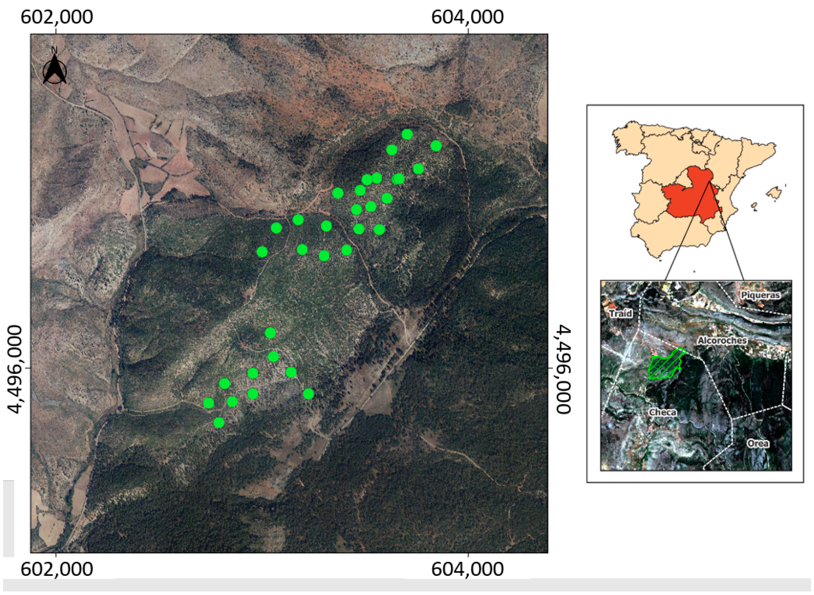
The burnt area affected by the forest fire is located in the surroundings of the Municipalities of Chequilla, Checa, Alcoroches, and Traid, in the province of Guadalajara (Spain).
This area has a typical temperate oceanic climate, Cfb by Köppen, without a dry season and a warm summer, where the average temperature during the coldest month is barely below 0 °C, the annual average temperature is above 22 °C, and up to 7 months average above 10 °C. Chequilla records an average annual temperature of 9.1 °C, as well as total annual rainfall of 703 mm, and it lies at 1,355 m.a.s.l. The soils are mainly schist or slate-based schist with some areas dominated by sandstone and quartzite.
The fire started on 1 August 2012 and finished on 4 August 2012, affecting up to 1151 ha, of which 788 ha was included in the forest category mainly dominated by Pinus sylvestris L. with some individuals of Pinus nigra Arnold. and Quercus pyrenaica Willd. in the understory.
It was a crown fire affecting every green needle of the Pinus sylvestris L. and Pinus nigra Arnold., and all the pines died. After the fire, every pine was cut and harvested, extracted away. Together with the crown fire burning all the pines, fire affected the second story composed of Quercus pyrenaica Willd. Regarding the severity, all the pines and shrubs were burned.
In 2020, the burnt area was naturally regenerated only in 136.52 ha composed of
Quercus pyrenaica Willd. as coppice and shrubs of
Cistus laurifolius L. and
Genista florida L., representing a typical association of degraded forest according to Ruiz de la Torre [
20]. This regenerated area of young oak coppice covering 136.52 ha was the object of our study. The shrub structure after the fire could, in principle, be considered homogeneous in comparison with the neighboring areas that were not burned. However, different development stages of the shrub vegetation were found due to different species composition, from shrub areas simultaneously displaying low and high development to other areas with only short (
Cistus laurifolius L.) or with tall shrubs (
Genista florida L.).
The center of the studied area is located at 604,700, 4,495,300 coordinates referenced to the UTM 30 TWL zone over datum WGS-84, corresponding to 40°36′7″ N, 1°45′45″ E. Next to this area, significant forest structures corresponding to
Pinus sylvestris L. (DGCN, 2006), burned areas, and agrarian and urban settlements can be found (
Figure 1).
2.2. Satellite Imagery
Sentinel-2 imagery was used, taking advantage of its availability, high spatial resolution, and processing level. The image was downloaded in a Level2A reflectance (at the bottom of the atmosphere) [
21], and no further post-processing of the image was performed.
The image acquisition and the field sampling data were contemporaneous (
Table 1). Considering that the annual biomass growth is achieved in the spring and summer months and assuming only a unique total annual rate (as a discrete value, not as a continuous increase), just a single satellite image, the closest image to the summer solstice of 2020 was used to obtain the final biomass map.
2.3. Sampling Method and Evaluation
Concerning sampling methods in shrublands, many methodologies have been suggested. For example, the line intercept method developed by Canfield [
22] is a technique that was employed to estimate cover in the grasslands of southwestern USA. It is the most used and adapted for rangeland inventory and monitoring applications, including the assessment of biomass in burned areas in a shrub–grassland mosaic [
23]. However, due to the aim of the actual research of reducing the sampling cost and maximizing the representativeness of the database, a random inventory was developed.
Circular 15 m radius plots were randomly established along predefined transects ensuring a minimum distance between them of at least 100 m to avoid overlapping of the Sentinel-2 pixels related to the plot.
For each one of the 32 plots sampled, the species composition was checked to ensure that it belongs to the shrub formation composed of Quercus pyrenaica and Cistus laurifolius, and the soil cover and mean height of the structure were measured. The field campaign was performed between 22 June 2012 and 24 June 2012.
To ensure the reliability of the sample selection procedure, the Monte Carlo method was applied [
24]. This method proceeds with a data analysis based on random sampling to generate the values for the probabilistic components. It compares the sampling with simulated databases to evaluate the representativeness of the sampling, regardless of the small number of plots sampled. Moreover, this method combines statistical concepts such as random sampling with the generation of pseudo-random numbers, and it is based on systematic sampling of random variables.
An evaluation of the radiometric value distribution was performed following the Monte Carlo procedure, comparing the NDVI distribution values of inventoried plots against the NDVI distribution against a random surrounding area of 10 × 10 km. As the number of plot pixels and the area of study were completely different, it was not statistically consistent to compare two NDVI histograms. Then, a comparison between the NDVI cumulative frequencies of both distributions was carried out to benchmark the actual frequency to a randomly shifted sampling pattern.
Thanks to this method, (i) a cumulative frequency of the N pixel of NDVI values corresponding to the sampling was computed. Afterward, (ii) the cumulative frequency of NDVI on a randomly shifted sampling design was computed, and then step (ii) is repeated 199 times with 199 different random translation vectors.
This method provided a total population of N = 199 + 1 (actual) cumulative frequency on which a statistical test with a significance level of 0.05 was applied: for a given NDVI level, if the actual plot density function is located between two limits defined by the five highest and five lowest values of the 200 cumulative frequencies, the null hypothesis is not rejected because there are no differences between both samples; otherwise, it is rejected. In the first case, both NDVI distributions are supposed to be equivalent, assuming those NDVI distributions between the area of study and the sampling plots.
2.4. Allometric Equations
An allometric equation for shrub formation composed of
Quercus pyrenaica and
Cistus laurifolius was applied [
25] Equation (1).
where soil cover of the vegetation is taken as a percentage (%), and mean height of the formation is taken in cm.
2.5. Carbon Sequestration Assessment
The total biomass stock recovered after a forest fire is considered as carbon sequestration in a CO
2 equivalent form (CO
2 eq.). First, a carbon fraction of dry biomass of 0.4799 was calculated according to previous studies [
26,
27]. Then, the molecular weight of the CO
2 and the stoichiometric relationship between carbon and CO
2 were considered to achieve the total amount of CO
2 eq. This approach shows a transforming coefficient from biomass to CO
2 eq. of 1.759.
2.6. Data Analysis with Gaussian Process Regression (GPR)
Gaussian process regression (GPR) models are nonparametric kernel-based probabilistic models. While linear regressions estimate the error from the database itself, a GPR generates a response from an interval of variables of the training data and a new vector as input by introducing variables from a Gaussian process.
The main assumption is that a set of random variables at any finite combination of them are distributed along the Gaussian curve, and then any number of observed variables are also distributed as Gaussian. Consequently, a GPR model is a probabilistic method; thus, it is possible to predict the outcome intervals from training models. Moreover, the results do not fit a line of responses but lie over a probability interval [
19].
The covariance function between input and output variables shows the similarity between them. This kernel function and its mean (adjusted to zero for simplicity) define the GPR [
28]. In this study, a kernel function with a separated length scale for each predictor was applied over the data, where an automatic relevance determination (ARD) method was used to order the inputs according to their importance [
29].
GPR is a very suitable method for remote sensing analysis as it is not limited by the large number of parameters needed for the implementation of methods such as neural networks [
30], and its computation requirements are less demanding than those based on pixel-by-pixel inversion methods such as the lookup table (LUT)-based radiative transfer model (RTM) [
15]. However, GPR has not yet been tested on areas requiring a huge effort of inventory to simplify the field data.
GPR computation [
31] was trained with Sentinel-2 spectral bands 2 to 8A (490 to 865 nm), both included, along with SWIR bands 11 (1610 nm) and 12 (2190 nm) as inputs, whereas total biomass represented the output. No additional synthetic band was created because nonparametric methods could extract all the relevant information of the bands without user intervention.
Field data were randomly split into six subsets with well-distributed values of biomass. Moreover, five subsets were used for algorithm training in each iteration, and one subset was utilized for the result validation. This procedure was performed six times in total so that each subset was used once as a validation group during the statistical analysis. The obtained estimations and corresponding errors resulted from the average of the six iterations. The aim of the iterations was the generation of every possible combination between training and validating subsets to make the validation more robust by using all the subsets for this purpose. The performance was evaluated with the absolute root-mean-square error (RMSE) and the coefficient of determination (R2) as overall indicators of accuracy.
To understand the fit between observed and predicted values, a major axis regression (MAR) line corresponding to the well-adjusted slope was included [
32]. Although it has been demonstrated that, for adult forest structures, it is necessary to split the reflectance values according to their features [
33], the post-fire regenerated shrub structures were tested as a single class.
3. Results
3.1. Inventory and Database
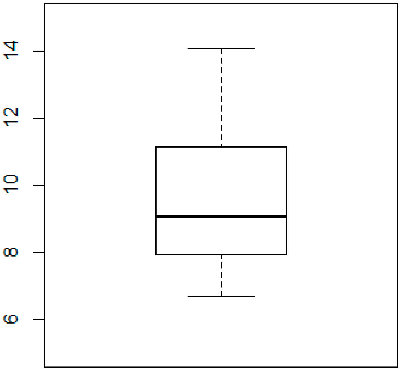
After the random application of the sampling method, great variability of biomass including stories and weight was observed (
Figure 2 and
Table 2) when characterizing a post-fire shrub structure with just a limited number of plots (32 sampled plots). CO
2 eq. was calculated for the database (
Table 2).
All 32 plots ranged between 50% and 95% fractional cover with 25 plots with at least 70% fractional cover. The height of Quercus pyrenaica Willd. ranged between 0.6 and 1.9 m. The plot area with a radius of 15 m was shared with Cistus laurifolius L. and Genista florida L., but typically with a lower height than that of Quercus pyrenaica Willd.
For the shrub biomass sampling, the mean (9.488 Mg·ha
−1) was slightly higher than the median value (9.06 Mg·ha
−1). The difference between the median and the third quartile (11.127 Mg·ha
−1) was higher than that between the median and the first quartile (7.947 Mg·ha
−1). As a result, the database displayed a slightly positive skewed distribution but was close to a normal one. The range of 6.7 to 14.040 Mg·ha
−1 was not especially wide for a shrub structure of the same age. In addition, remarkable differences could not be found via a visual inspection. However, even with a minor asymmetry in the distribution of the biomass, these values and ranges were also reported by other authors [
12]; consequently, the sampling could be accepted as adequate for this study.
3.2. Field Sampling Evaluation
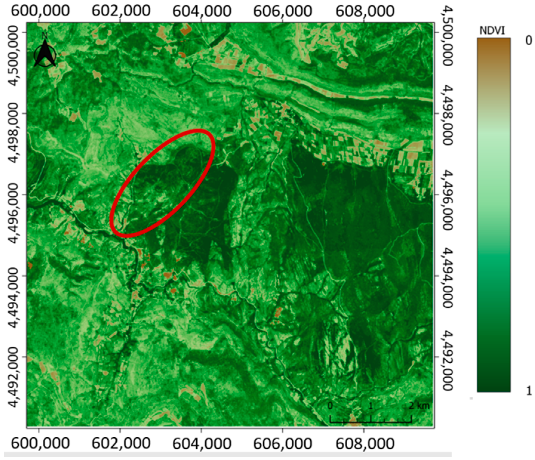
Once biomass values were well distributed, an evaluation of the radiometric value distribution was performed by comparing the NDVI distribution values of inventoried plots against the NDVI distribution over the whole scene employing the Monte Carlo procedure (
Figure 3). For a methodological demonstration, a global area of 10 × 10 km was selected, including the burned area. Nevertheless, this burned area represented only around 5% of the total territory included in the study area and a wide surrounding area that was not burned.
The Monte Carlo procedure was performed to avoid any extreme value or outlier in the sampled plots. Its application could also confirm that the included reflectance values did not promote any bias, and that no imagery processing issues were present in the database.
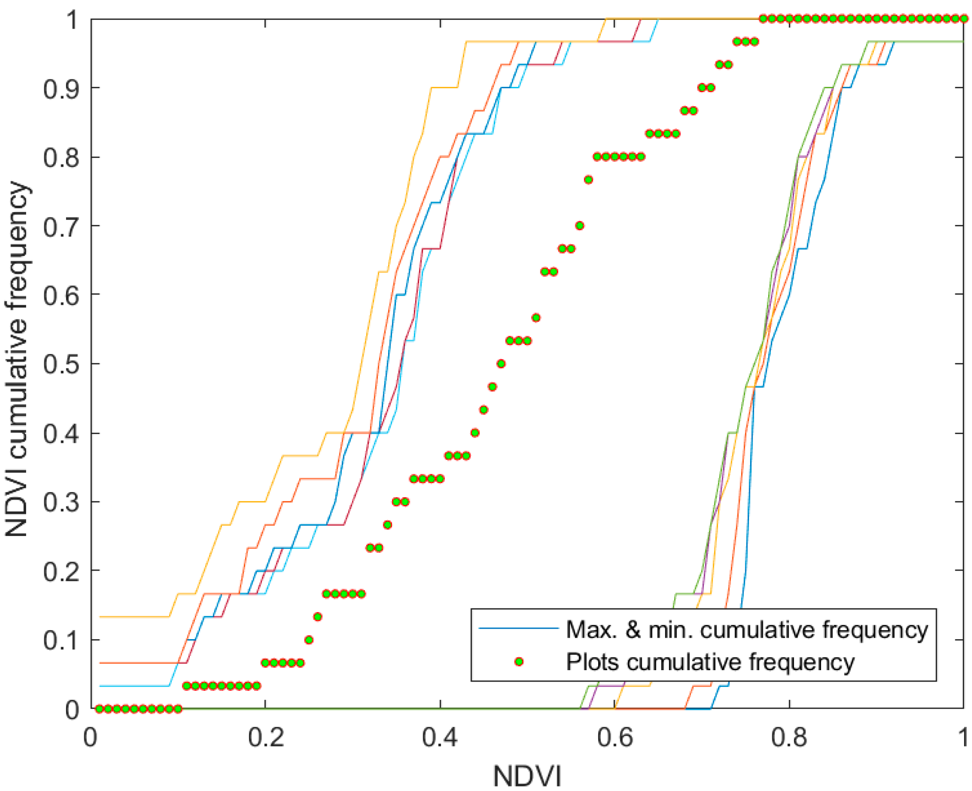
Figure 4 displays that plotted values (green dots) were rather representative of the other pixels in the whole area, and that any bias was forced. After iterating groups of random pixels against sampled pixels, it can be noted that the NDVI value distribution for the field sampling agreed with the values of the study area. Moreover, real and simulated distributions were equivalent, as shown in
Figure 4, with the NDVI values of the plots ranging between 0.44 and 0.80. It was assumed that lower values were not related to the forest due to the high soil cover fraction values of the plots (0.5 to 0.95).
This wide area of 10 × 10 km clearly shows that NDVI values were very similar for both burnt and recovered areas, as well as other non-disturbed forest parts.
3.3. Biomass and Carbon Assessment
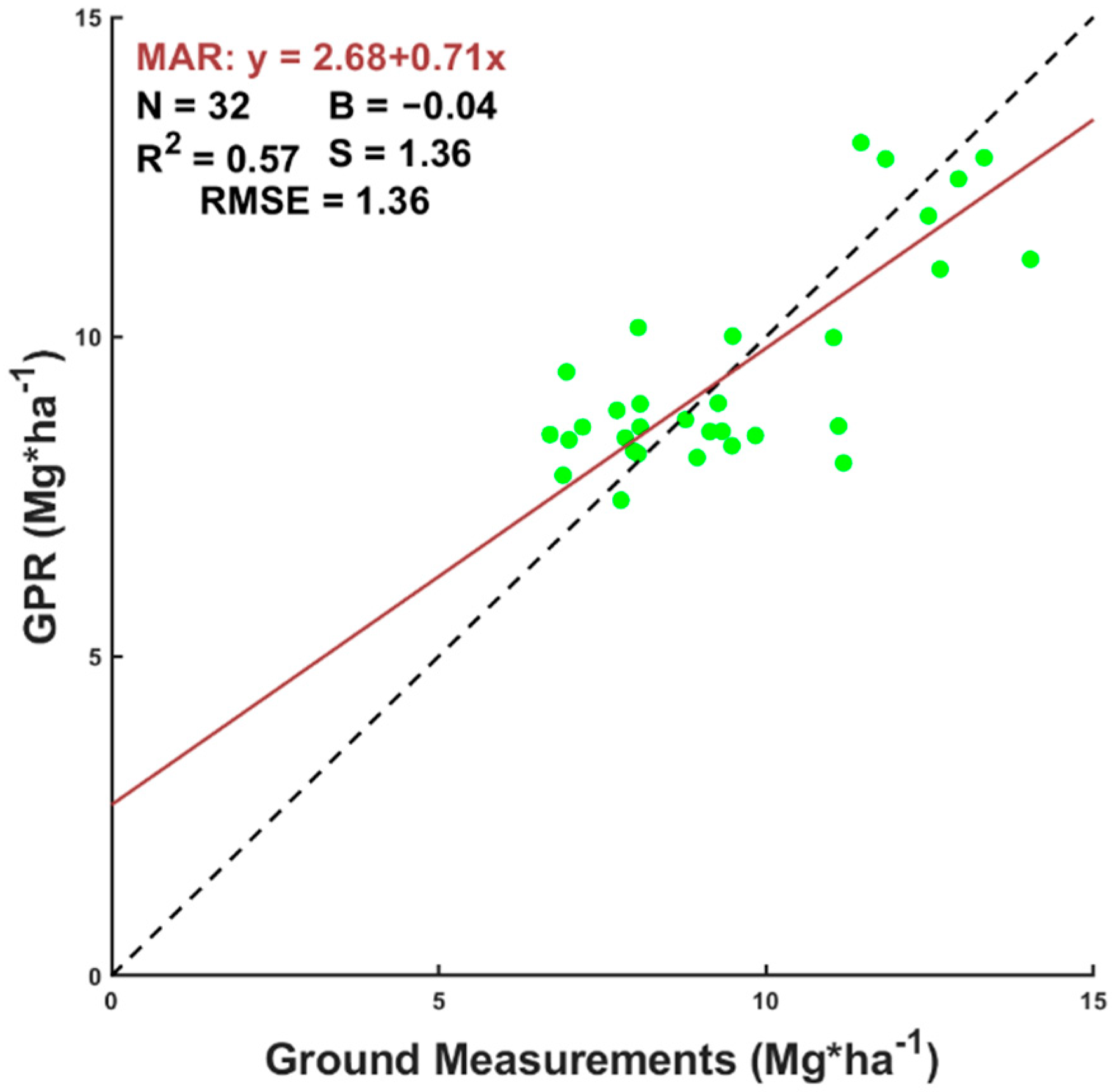
Figure 5 shows the scatterplot between the best-fitted model obtained by GPR and biomass ground data for the oak coppice forest of
Q. pyrenaica Willd. with other shrub species. Using all these points for training a GPR with Sentinel-2 data, the
R2 between those estimated values against field data could account for up to 57% of the variability of the forest.
The error, evaluated as root-mean-square error (RMSE), accounted for 1.36 Mg·ha−1 in the gathered biomass range of 6.7 and 14.040 Mg·ha−1, representing a relative error between 9.75% and 20.4% in the biomass assessment. In some cases, biomass was underestimated, whereas, in others, it was overestimated.
The linear MAR fit between predictions and ground values revealed fitted slopes (0.71) and a small offset where the y-intercept was roughly 2.7 Mg·ha
−1, a value that shows a barely uncovered terrain (
Table 3). All these results indicate that the combined use of random field and low-intensity sampling together with a minimum segmentation of the database, which was ensured by equivalent real and simulated distributions, could provide satisfactory results for forest management purposes and carbon accountability by using probabilistic models applied to remote sensing imagery of Sentinel-2.
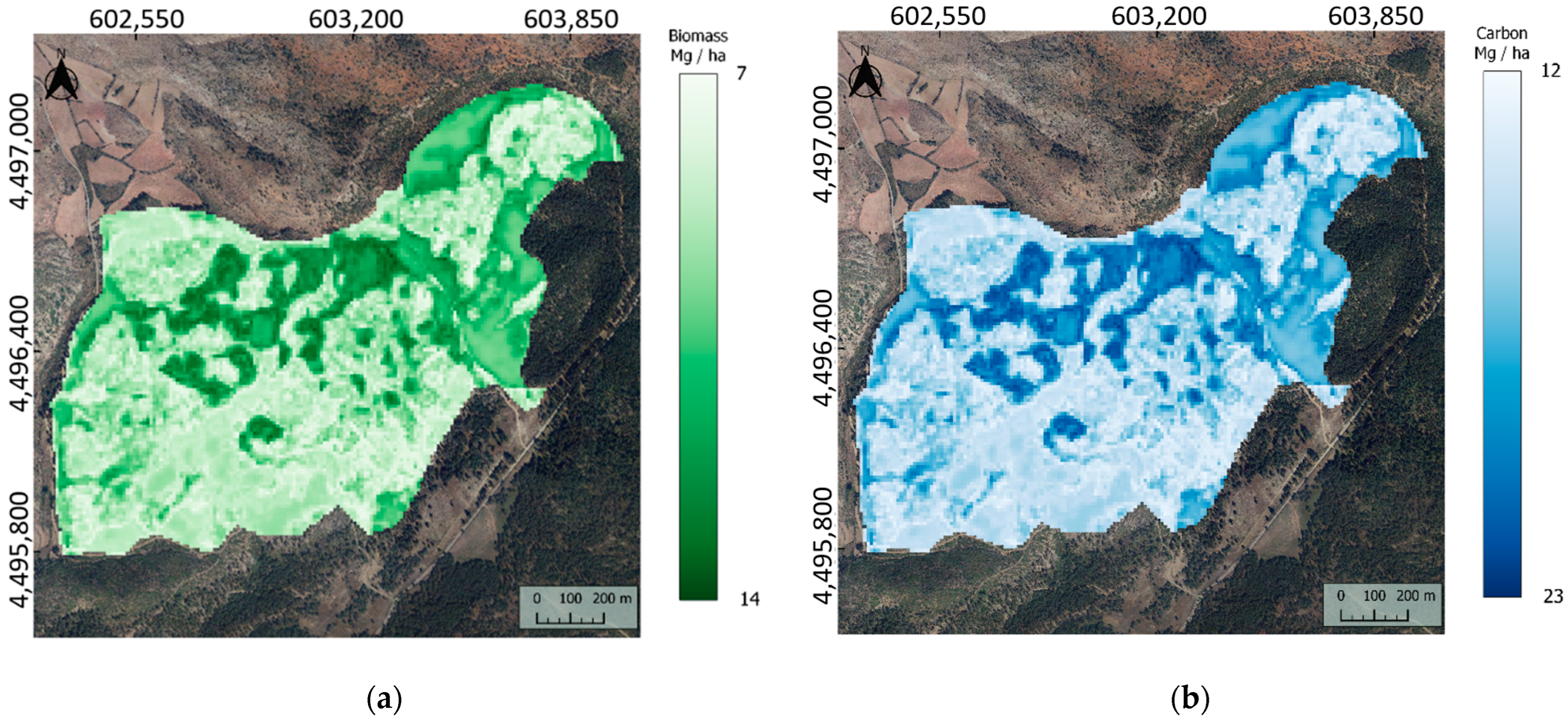
Next, the general algorithm obtained from the GPR was applied over the corresponding area to determine the total biomass in the post-fire regenerated area (
Figure 6a). Additionally, the relationship between the biomass and the CO
2 eq. was considered to estimate the total sequestrated carbon in the next 8 years after the wildfire (
Figure 6b).
In the area of 136.52 ha, a total sequestered carbon of 2307.37 Mg of CO2 eq. was estimated for the young oak coppice during the natural recovery period, corresponding to an average carbon sequestration of 2.112 Mg CO2 eq·ha−1·year−1.
3.4. Application of GPR over Non-Burned Areas
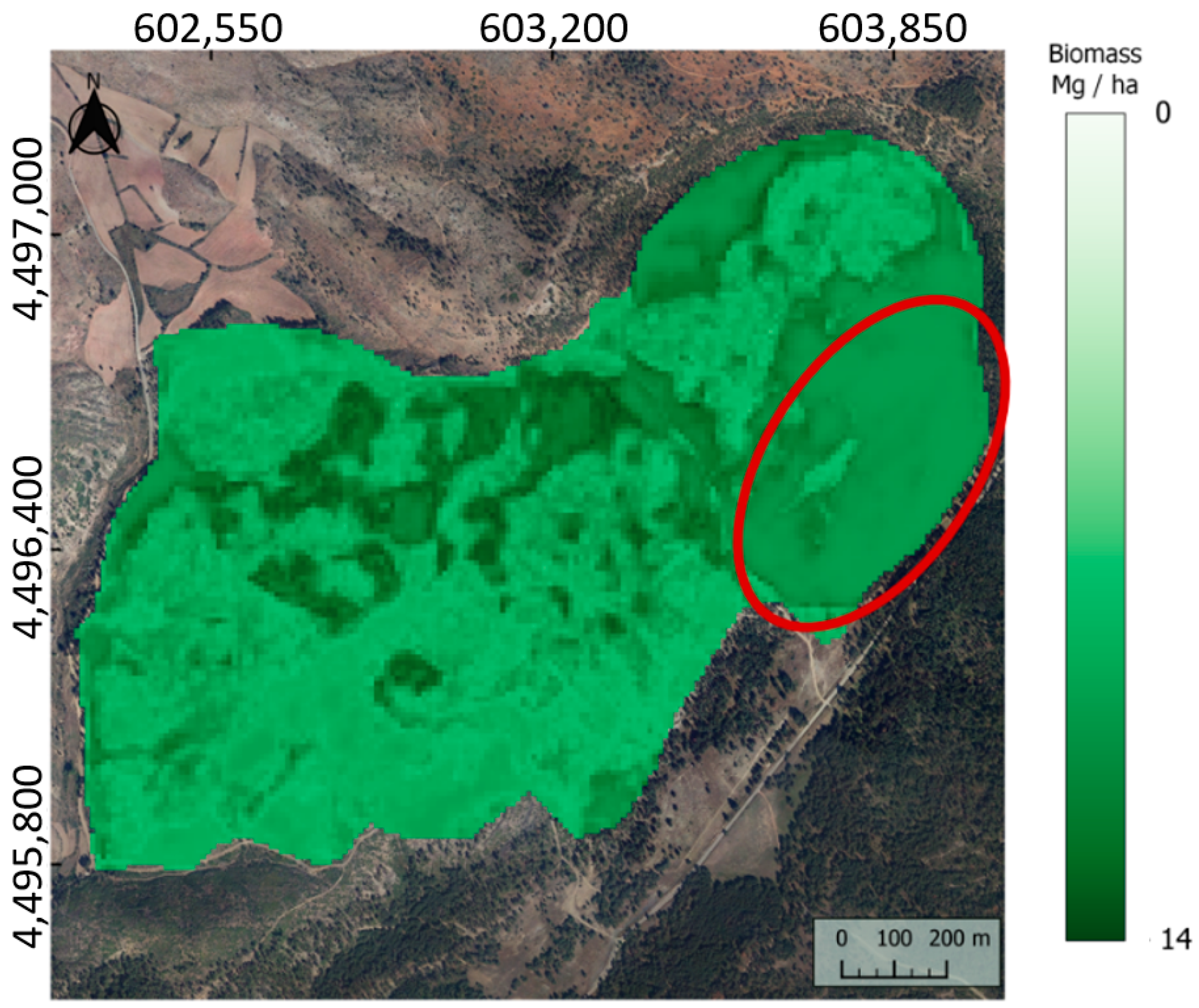
Although the GPR was trained for a specific forest structure, its application over another type of forest was also tested. After the application of the GPR methodology over the young oak coppice, an experiment was performed by applying the same routine over 14.8 ha of non-burned areas (
Figure 7). In particular, the affected area remained as a mature forest dominated by
Pinus sylvestris L.
GPR gave underrated values of biomass for a homogeneous mature forest of Pinus sylvestris L. When a specific algorithm for young oak coppice was applied over another forest structure, it was not able to distinguish the species, the structure, or the biomass differences.
4. Discussion
In this work, we proposed an operative and simple methodology for assessing biomass sequestration in post-fire regenerated shrublands.
This routine applied the nonparametric empirical method of Gaussian process regression over Sentinel-2 surface reflectance and forest inventory data obtained after fieldwork. In this way, carbon stock given as sequestrated CO2 eq. could be directly calculated as a function of the total biomass data.
This method was demonstrated to be reliable and cost-effective in temperate oak coppice forests with shrubs. Other methodologies have been purposed for accurate forest inventories, by traditional [
7] or even LiDAR means [
34,
35]. However, our approach requires a very low number of forest inventories. Specifically, for an area of 136 ha, only a sampling plot every 4 ha of regenerated coppice was enough to achieve an
R2 of 0.57.
Moreover, this regression method needs no explicit selection of spectral bands, avoiding an their hoc selection as GPR can extract the relevant information of each band. For this purpose, the spectral resolution of the MSI sensor of Sentinel-2 was adequate.
The biomass in this study ranged between 6 and 14 Mg·ha−1, and the RMSE obtained was low, showing a high level of determination found. Indeed, almost 60% of the variability of the forest could be explained using this method.
The error magnitude was low enough to classify each pixel within each class of fuel model [
4,
5] and improve the spatial segmentation because the representation of the results was accurate at Sentinel-2 pixels with a 10 × 10 m resolution.
This methodology provided precise information of biomass and carbon content in young oak coppice in agreement with previous studies, which can be used as a major improvement of the accuracy for the assessment of carbon sequestration [
36].
Once carbon sequestration was estimated for the whole area of study and assuming a linear annual growth of young oak coppice until a dominant height of 5 m [
37], an average carbon sequestration of 2.112 Mg·ha
−1·year
−1 for this shrub structure was obtained, in agreement with previous carbon quantification studies [
11].
Affordable methodologies have been proposed for shrubland biomass assessment at large scales, taking advantage of remote sensing technologies [
8]. In this study, remote sensing was validated to detect differences in a small area of shrub post-fire structure that could be in principle considered homogeneous, providing accurate information about its evolution and carbon sequestration capacity.
After a fire occurrence, different development stages of the shrub vegetation can be found: areas with low shrub development, others with high shrub development, and areas with only short shrubs or only high size shrubs. Regardless of the stage and structure, remote sensing and field data were used to estimate biomass in shrub areas in Portugal [
8] and California [
38], to identify changes in aboveground biomass after fire in the Amazon [
39], and to evaluate vegetation recovery after fire in Siberia [
40]. In this line, the methods can be considered suitable for the proposed objectives of the manuscript as it accurately estimated the carbon stock in small coppice areas.
In a random area of 10 × 10 km surrounding the study area, it was shown that the distribution of NDVI values was equivalent for both recovered and unaffected forest areas. Thus, for a precision analysis of the post-fire evolution, a segmentation needs to be performed to not commit over- or underestimation of the biomass.
Consequently, the application of trained GPR for a specific forest structure over other forest types must be avoided, as it will create confusion in the assessment of any biophysical variable since reflectance values were quite similar for both vegetation groups, and only a clear segmentation of the target areas could resolve this issue.
Although some spectral methods for land use and classification after a forest fire have been proposed for a segmentation of the areas [
3], the use of ground-truth maps is recommended to apply algorithms over the same forest structures. According to [
11,
12], segmentation of the classes is necessary to avoid errors in the biomass assessment, as reflectance values are not valid to split structures in tiny areas.
For an accurate biomass assessment, land segmentation is required because, if any error of land classification is made, GPR will under- or overestimate the results, as shown in an experiment over 14.8 ha of Pinus sylvestris L.


 ,
, 


