
Ecosystem Carbon Stocks and Their Annual Sequestration Rate in Mature Forest Stands on the Mineral Soils of Estonia

1
Institute of Agricultural and Environmental Sciences, Estonian University of Life Sciences, Kreutzwaldi 5, 51006 Tartu, Estonia
2
Institute of Forestry and Engineering, Estonian University of Life Sciences, Kreutzwaldi 5, 51006 Tartu, Estonia
*
Author to whom correspondence should be addressed.
Forests 2022, 13(5), 784; https://0-doi-org.brum.beds.ac.uk/10.3390/f13050784
Submission received: 19 April 2022
/
Revised: 13 May 2022
/
Accepted: 16 May 2022
/
Published: 18 May 2022
(This article belongs to the Special Issue Soil Organic Matter and Nutrient Cycling in Forests)
Abstract
:Mature forest ecosystems are the most considerable reservoir of organic carbon (OC) among terrestrial ecosystems. The effect of soil type on aboveground OC stocks and their annual increases (AI) of overstorey tree, understorey tree and ground vegetation layers in Estonian forest phytocoenoses with mature stands on mineral soils were studied. The study enfolds nine mineral soil groups, which are characterized by their phytocoenoses composition, soil cover properties and tree stands’ taxation data. An assemblage of soil and plant cover or plant–soil system is the main focus point in explaining causal and quantitative sides of ecosystems functioning. Surface densities of OC stocks in aboveground phytomass of forests varied significantly in the range of 52–100 Mg OC ha−1. High AI or productivity (4.8–5.5 Mg OC ha−1 year−1) is a characteristic of forest ecosystems formed on leached, eluviated and pseudopodzolic soils. Forest ecosystem ground vegetation, which is an important ecological indicator, fulfils vacant ecological niches with herbs and/or mosses (up to 0.50 Mg OC ha−1). The variation of ecosystem OC stocks and their AI by soil type should be taken into account in regional OC stocks and its annual increase estimations.
1. Introduction
Forest ecosystems (as assemblages of phytocoenoses with functioning soil covers) are the most important sink and reservoir of organic carbon (OC) among terrestrial ecosystems [1,2,3]. Significant OC stocks of temperate and boreal forests are located in aboveground overstorey tree phytomass, whereas the storage of OC in superficial soil layers (mostly in humipedon) may be independent of soil type and it can be both lower or higher than that of the aboveground OC storage [1,3,4]. Soil cover composition and functioning are the main drivers of ecosystem net productivity [5]. Forest ecosystems on mineral soils have a relatively higher capacity to allocate and store OC as an aboveground pool, while in contrast, OC in organic soils is stored mainly in soil cover and to a lesser extent in phytomass [2,6,7]. The local variation of mineral soil properties can be very different, which influences substantially the accumulation of OC in phytomass and its annual production.
Soil cover, being the most important component of terrestrial ecosystems [2], is in relatively diverse hemi-boreal conditions. When managing and assessing soil covers, their properties and quality diversities should be taken into account [3,7]. Dependent of soil forming conditions, soils of various genetic type may be presented, each with different moisture conditions, skeletal fraction fine earth texture, organic matter sequestration (or capture, removal accumulation) into the soil and other [8]. Soil cover properties depend not only on the OC sequestration capacity in the soil, but also on the turnover rate between soils and plants [5,9]. Since ancient times, land use of various regions was arranged in perfect harmony with the soil type properties of an area [10]. As a result of this, the existing soil covers have been divided into arable, forest and grasslands, among which different kinds of rangelands may be presented. To the last group belong soils which are unsuitable for any kind of agricultural management, as well as areas taken under buildings, routes and other in the process of soil sealing.
Dependent on soil types presented in soil covers, variegated site (growing) conditions for plant covers and living organism association networks assembled with them exist [5,11]. Soil covers are functioning in assemblage with plant covers as a main energy source for soil cover [12]. The feedback of plant cover influences mainly the humus cover (or epipedon) layer of the whole soil cover [13,14]. In light of this, it seems appropriate to use the term ‘’plant–soil system’’ [10,15]. An assemblage of soil and plant covers is the principal focus point in explaining the causal and quantitative sides of ecosystem functioning [11]. The fabric and functioning plant–soil system (as a prevailing part of the ecosystem) depends on both soil type and mode of land use [16,17]. The same soil type may be independent from the land use form, differing from each other by their fabric humus covers (pro-humus forms) [13]. Despite land use changes, the main properties of subsoils do not change to a substantial extent, despite profound alterations that happened in humus covers [18,19].
The capacity of different forest soil types to accumulate OC in plant cover is expedient to describe in steady-state conditions, i.e., in mature forests [3,4]. The OC stocks and the production of plant cover in mature forest express maximum storage, and therefore, could be a good proxy to test the capacity of CO2 uptake potential between different soil types [20,21]. Previous studies have focused on the site type classification [3] to assess the capacity of mature forest in OC fixation, but site type ordination generalized several soil types [22] and the actual soil variation was not taken into account with such approach.
We studied OC turnover in a plant–soil system in mature coniferous and mixed coniferous–deciduous forest ecosystems formed on mineral forest soils in Estonia. Established on different mineral forest soil research sites (total of 193), they enfold approximately 63% of all mineral forest soils dominated here.
The main aims of the present study are as follows: to characterize the OC sequestration capacity of mature coniferous and mixed coniferous–deciduous forest stands with assembled ground vegetation and understorey tree layers; to characterize quantitatively annual increases (AI) of OC in main aboveground constituents of studied forest phytocoenoses; to characterize soil covers (or sola) from physical, chemical and biological aspects, giving special accent to soil organic matter of the studied forest ecosystems; to analyze forest phytocoenoses aboveground constituents and different soil cover layer structures.
We hypothesize that the total amounts of phytomass and their annual increases in mature aged forest ecosystems depend on the remarkable extent of the ecosystems’ soil cover texture and their species composition.
2. Materials and Methods
2.1. Research Sites
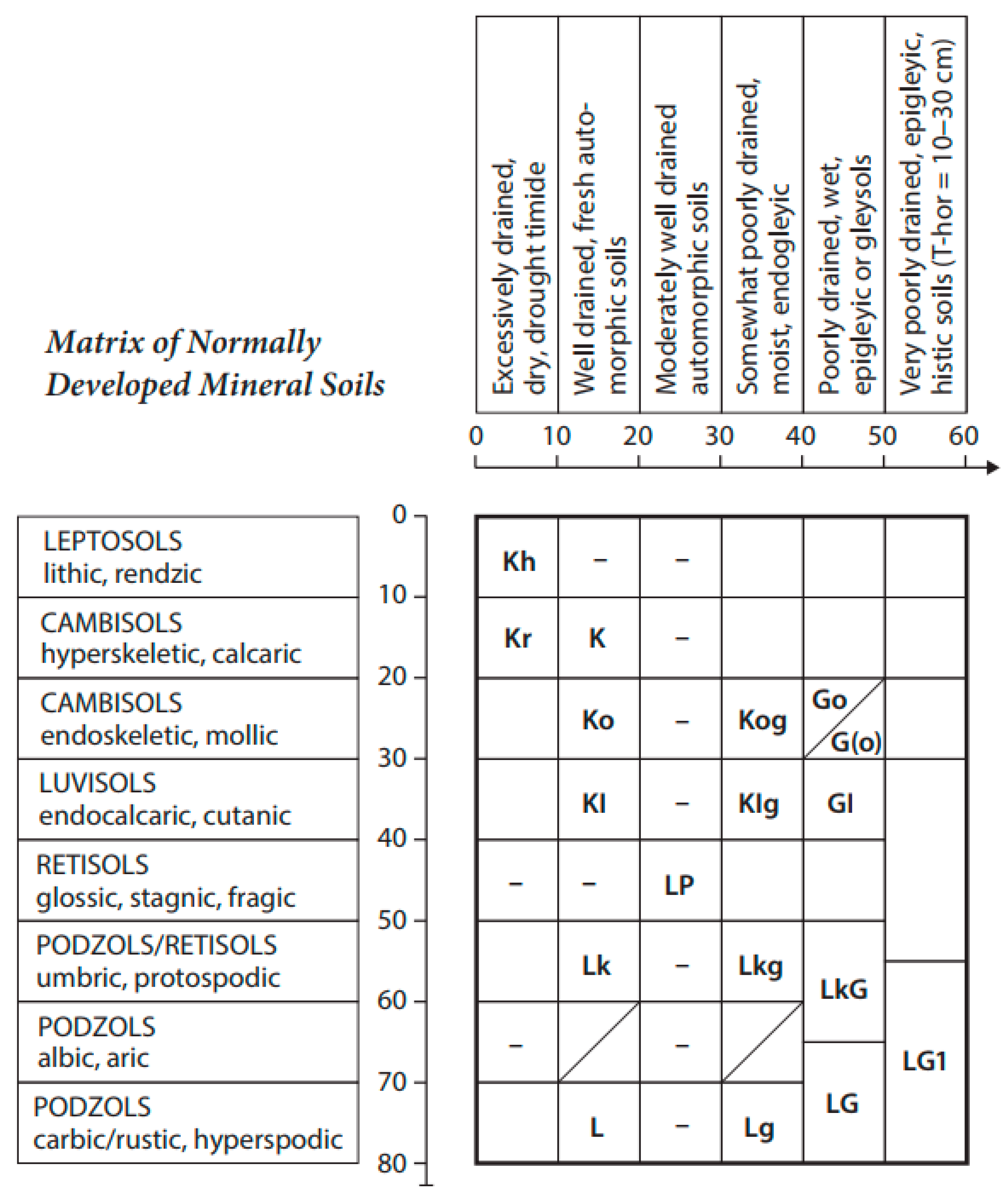
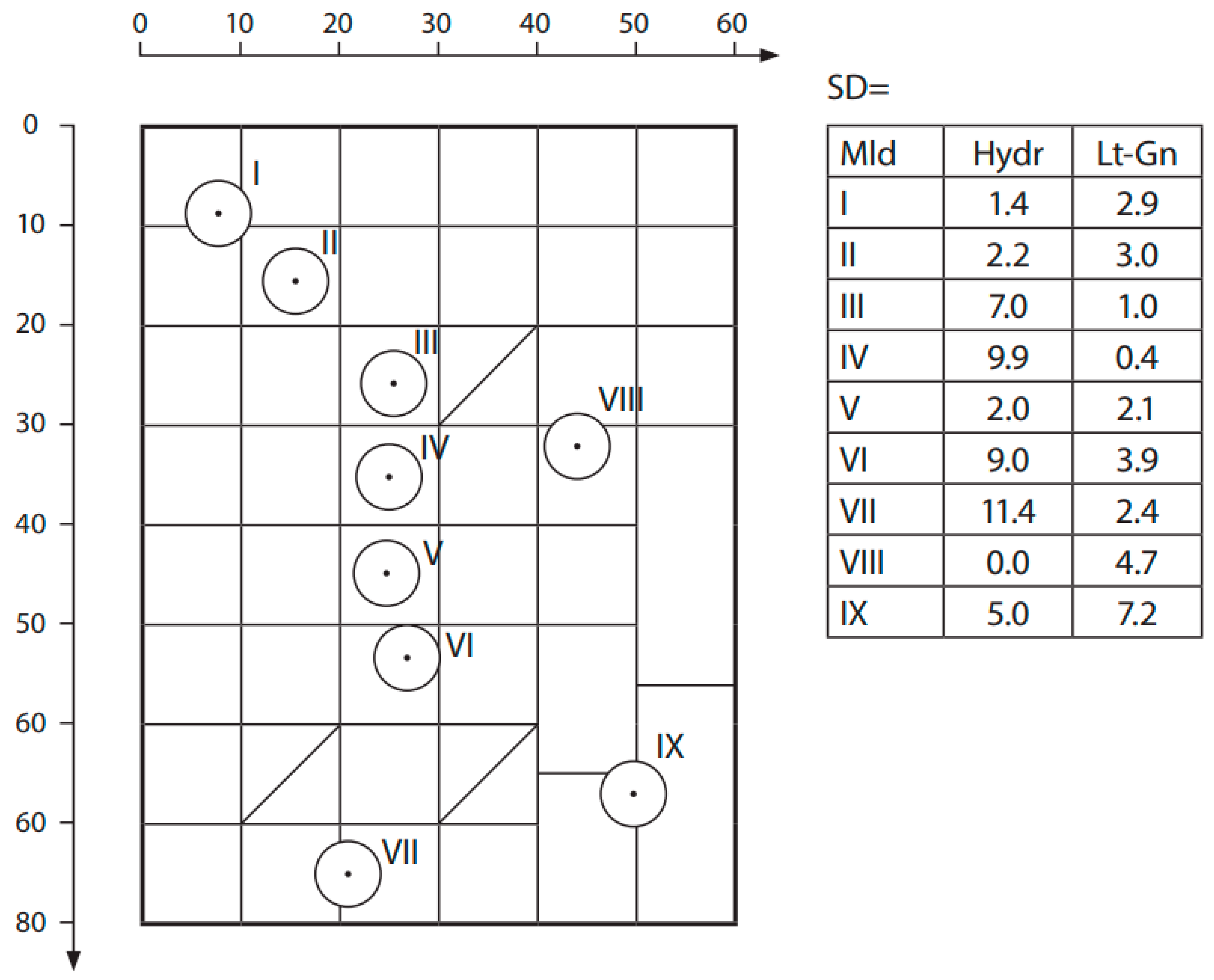
The main part of the quantitative data for the present work originates from the database “Pedon” formed between 1967−1995 and updated 1999−2002 at the Chair of Soil Science of the Estonian University of Life Sciences. The current study analyzed 193 forest research sites or forest ecosystems. Pedo-ecological information’s complex of ecosystems (phytomass areal density and AI of the main phytocoenosis compartments, stands taxation data, constituent structure of aboveground phytomass and data on soil cover or solum properties) was divided into nine soil groups. These groups enfold one (two groups) or two or more soil species. The pedo-ecological locations or taxonomical distances for each of these nine soil groups are given in Figure 1. Soil group (I–IX) codes and names are given after Estonian soil classifications [23], whereas their concordance with World Reference Bases for soil resources (WRB) [24] is seen in outlines on the scalars of the Estonian soil matrix table (Figure 1).
The dry weight of phytomass and the annual increase of different phytocoenosis compartments were determined according to the International Biological Programme (IBP) methods [25,26,27]. The overstorey tree stem phytomass was determined (from 76 research sites) with model trees, whereas their AI was determined by taking increment cores with increment borer. The phytomass and AI of tree branches and foliage were determined by model branches by taking every tenth branch for spruce and every fifth branch for pine and birch.. In the course of model branch analyses, the fractions of first and second order branches, last year`s sprouts and their needles or leaves were separated. In the case of pine and spruce, the needled branches (aged 2–7 years) were separated additionally. The average AI of all branch fractions was determined based on the fraction age. The phytomass of dominated understorey tree and shrub layer plant species was determined by using allometric models composed of the base of a tree diameter at 10 cm from the soil surface and their areal densities. The average AI of separated fractions of understorey layers was determined on the basis of each fraction age. The determination of ground vegetation phytomass was done by using sampling plots. In the case of herbs, the size of the sample plots was 0.5 × 1.0 m (0.5 m2), but in the case of mosses and forest floor, it was 0.25 × 0.40 m (0.1 m2). The AI of the herb layer was calculated as the sum of its different plant species` maximal phytomasses. For the determination of the moss layer AI, the fractionation of the presented layer dominating moss species models was analyzed.
2.2. Additional Explanations of the Used Terms
- -
- In the actual work, only mineral soil mature forest ecosystems’ productivity indices (as an assemblage of phytocoenosis and soil cover) are treated.
- -
- Phytocoenosis is the main component of the aboveground part of the ecosystem enfolding overstorey tree, understorey tree, shrub, herb and moss layers.
- -
- Plant–soil system is the association of plant and soil covers and the focal point in the functioning of the ecosystem.
- -
- Phytomass, known as plant biomass, is used here for a more exact separating of the plant origin biomass from microbial, animal, etc., biomasses.
- -
- Organic carbon, as a term, is acceptable to use for both plants’ and soils’ carbon of an ecosystem as this excludes soil carbon with mineral origin.
- -
- Soil cover or solum, is formed mainly by soil forming processes proceeded in the superficial layer of a landscape and consists of a humus cover (including forest floors) and subsoil.Soil species is the main taxon of Estonian soil classification identified by soil-forming processes.
- -
- Physical clay, separated by the Katchinsky system, is the assemblage of mineral soil particles with a diameter <0.01 mm [28].
2.3. Characterization of Soil Covers
Soil is a prerequisite in the forming of phytocoenoses and among tree stands. We support the statement that soil cover properties are determined by the composition and productivity levels of phytocoenoses. Therefore, it is expedient to start treating the ecosystem’s properties from the soil cover, which is the dominant compartment of terrestrial ecosystem aside from its phytocoenosis.
The Estonian mineral forest’s soil cover thickness is dominantly in limits of 28−93 cm (Table 1). Good physical conditions for high productivity are observed at soil covers in which the fine earth mass exceeds 10,000 and physical clay 2000 Mg per hectare. The specific surface index is the highest (>105 400 ha ha−1) in soil covers which contain clay and great amounts of organic matter.
Skeletal calcareous soils are saturated by basic cations (>90%); however, a low saturation stage (<50%) is a characteristic of Podzols. The main factors which determine the soil cover`s cation exchange capacity are contents of basic cations and soil organic matter. The hydrolytic and exchangeable acidities are uniformly higher in podzolized and saturated moisture soils.
Soil organic matter amounts are remarkably high (180−250 Mg ha−1) in calcareous and wet soil covers (Table 1). The summarized C:N ratio is the largest (>20) in Podzol soil covers. An essential factor in the formation of this are the high amount of soil organic matter in their forest floor.
2.4. Evaluation Status of Tree Stands
The stand-taxation data of research sites given by soil groups are essential for the characterization of forest states and also for the indirect estimation of carbon amounts (Table 2). The average stand ages range between 78−99, with the sole exception of group IV, which has an average age of 64 years. According to the Estonian stand age classification of coniferous forests, the prevalent amount of stands belongs to mature forest classes due to their age, i.e., the clear-cut age for coniferous tree species (Scots pine and Norway spruce) in managed forests is between 60–120 years [29]. Due to the stocking level of tree stands, the studied sites are practically similar, varying from 0.6 to 0.8 from the standard stand density (1.0). The reliable differences between stand volumes, which are characterized quantitatively by basal area at breast height and stock of stem, are statistically tested and are, by their characteristic tendencies, similar. On podzolized, more acidic soils, Scots pine stands are dominating, but in the case of calcareous soils, the prevailing role belongs to the Norway spruce stands. The used practical forest management stand quality classes vary from III to I, whereas the average quality class is II, 6. A good indicator for the characterization of forest stands is their location on the soil matrix (Figure 2). The positioning of soils on the matrix by their moisture conditions and litho-genetic scalars is essential for the determination of both site and humus cover types.
2.5. Methodological Principles of Data Elaborating
All pedo-ecological analyses of quantitative data on OC in different aboveground compartments of forest phytocoenoses were calculated using coefficient 0.50 after a preliminary determination of phytomasses and their AI [19]. Therefore, the contents of carbon were not determined directly from different compartments of phytocoenosis but were (re)calculated it using a unique coefficient despite the existing differences between herbaceous (carbon content approximately 45%) and lignified (50%) phytomasses. The use of a unique coefficient (0.50) is justified by the fact that the lignified parts are dominating compared to other phytocoenosis compartments, as well as by the absence of systematized OC content for most compartments of forest phytocoenoses. Using a unique coefficient enables easier recalculation of preliminary data to more exact data.
Statistical analysis of data on phytomass densities and their AI, as well of data on stand taxation, quantitative characteristics of soil cover and structure of phytocoenosis components was performed by an one-way ANOVA and a Fisher test using the STATISTICA 13.2 software. To ensure that the parametric assumptions were met, the Shapiro-Wilk test for normality of residuals was conducted; residuals were visually inspected for homogeneity of variance. The level of statistical significance for all tests was set to p < 0.05.
3. Results
3.1. Organic Carbon Surface Densities in Different Compartments of Phytocoenoses and Soil Covers
Based on soil cover (treated by soil groups) properties, the surface densities of aboveground OC stocks in forest phytocoenoses in mature coniferous and mixed coniferous–decidious stands varied from 52 to 100 Mg OC ha−1 (shown in Table 3). The highest stocks of phytomass OC were observed on different kinds of calcareous (excluding skeletal dry) soils (59–92 Mg OC ha−1) and the lowest were observed on acid soils (52–59 Mg OC ha−1). The carbon amounts in tree stems are accumulating in a similar way, being in the limits of 44–75 and 47–50 Mg ha−1, respectively. The stand foliage OC ranged between 1.4–6.1 Mg OC ha−1 and the branches ranged between 3.5–15.6 Mg OC ha−1. Well-developed herb and understorey tree layers have been formed on calcareous soils (0.3–0.4 and 0.6–1.9 Mg OC ha−1, respectively); however, moss and shrub layers on acid soils were 0.7–2.2 and 0.2–0.6 Mg OC ha−1, respectively.
3.2. AI of OC Stocks in Different Compartments of Forest Phytocoenoses
AI of OC (Mg OC ha−1 year−1) in the aboveground part of mature forest phytocoenoses on different soil types varied from 2.2 to 5.5 Mg OC ha−1 (shown in Table 4). The highest productivity of phytocoenoses (4.8–5.5 Mg OC ha−1 year−1) was observed on leached, eluviated and pseudopodzolic soils with different moisture conditions. The AI of all other soil groups is under 3.3 Mg OC ha−1 or between 2.2 and 3.3 Mg OC ha−1. Similar differences are observed in the AI of OC sequestrated into stand stems (1.2–1.9 and 0.7–0.9 Mg OC ha−1 year−1, respectively) and foliage (1.0–1.6 and 0.5–0.7 Mg OC ha−1 year−1) of the aboveground part of overstorey tree layers.
Compared to the tree layer’s annual OC increment, different patterns are observed in the ground vegetation. Here, we see a compensation capacity (as ecological regularity) of the ground vegetation, by which the vacant ecological niches have been fulfilled, depending on topsoil properties, with herbs (up to 0.43 Mg OC ha−1 year−1) or mosses (up to 0.46 Mg OC ha−1 year−1). Only in Podzols, the AI of the shrub layer has significant importance (0.10–1.14 Mg OC ha−1 year−1). In mature forests, the understorey tree layer has a small annual OC accumulation capacity (0.04–0.28 Mg ha−1 year−1).
3.3. Allocation of Phytomass and AI in Forest Phytocoenoses
The aboveground phytomass densities of I and II soil quality class mature forests show that the main share of OC (96–99%) is located in the phytomass of the overstorey tree layer (shown in Table 5). With lower soil quality classes, the share of forest tree layers is lower (89–94%), whereas in most cases, the lower percentage is compensated by a higher share of mosses (4.1–5.4%). Although herbs and understorey tree layers have important indicative value, their share in the total forest phytomass is relatively small (<0.05–0.8% and 0.3–2.6%, respectively).
In the case of AI, the share of ground vegetation and understorey tree layers is higher, but the share of overstorey tree layers is lower compared to the phytomass superficial densities. Based on pedo-ecological conditions, the AI of herbs forms 0.8–14.7%, mosses form 2.0–27.6% and the understorey tree layer forms 1.2–6.0%, but the overstorey tree layer is 62–90% of the total AI. The share of foliage from the total phytomass ranged between 5.4–9.7% and its AI between 40–54%, being relatively stable among the studied soil groups. If the share of stand stem phytomass forms 70–81% of the total aboveground phytomass, then their role in the AI of the total phytocoenosis is relatively modest at 22–33%. The share of AI from aboveground phytocoenosis phytomass or OC amounts varied between 4.4 and 6.7%.
The OC ratios in the soil cover and in the aboveground part of phytocoenosis show that in most cases the amounts of OC in the soil cover exceed the quantities in the phytocoenosis by 1.2–2.2 times. The highest role of the forest floor’s OC in the functioning of forest ecosystems is characteristic to Podzols.
4. Discussion
4.1. Classifications of Different Forest Compartments as Valuable Tools in Sustainable Forest Management
In forest management practice, the proved tools are local classifications of forest site types [22], soils [23] and humus covers [13]. These classifications are valuable not only in pedo-ecological characterization forest growing conditions of an area, but also in the revision (mapping) soil cover properties and in the elaboration strategy for forest management [30,31]. The comparable study of these three tools has been shown that, although classification units and their determined indice borders to not coincide completely (far of 100 percent), each of them is necessary in the characterization of different aspects of forest growing conditions [13].
In this work, the amounts of OC in different compartments of ecosystems formed on III and IV soil groups are in good agreement with the same determined in Hepatica site type [3]. Good coincide between soil species and site types exists, as well as in relation with other mineral soil species. For example, the characteristics of Pseudopodzolic soils (group V) are similar with the ones in Oxalis site types, as well as Peaty Podzols are similar to Vaccinium ulginosum site types.
4.2. Pedo-Ecological Regularities in Allocation with OC in Phytocoenosis Phytomass and Its Annual Increment
We can confirm our main hypothesis mature coniferous forest stands’ OC stocks (Table 3) and their AI (Table 4) depend to a great extent on soil cover properties. Oppositely, a study of mature spruce forests in a hemiboreal region did not find variation in the soil conditions of ecosystem`s OC stocks [4]. The total OC stocks are in good agreement with stand-taxation data (Table 2). Forest stand species composition and soil cover types are determined not only by accumulated tree layer OC amounts and their AI, but also by the OC amounts and AI of ground vegetation (herbs, mosses, shrubs) and understorey tree layers. Thanks to these ecological regularities, it was possible to use ground vegetation as a valuable indicator in the characterization of sites’ forest growing conditions.
The role of ground vegetation constituents of phytocoenoses depends mainly on the presence of non-occupied ecological niches under the canopies of tree layers. It is evident that both stand composition and ground vegetation are differed substantially as compared to calcareous and acid mineral soil covers [3,13]. The increased role of the forest floor on acid soils from fresh to wet moisture conditions refers to the stagnation of biological turnover, which is proved by the thick forest floor on mineral soil layers (shown in Table 3). If on calcareous loamy soil, the dominating role belongs to the herb layer and the understorey tree layer, then on acid sandy soil, the moss and shrubs layers are dominating by their OC amounts. The structure of the OC densities and their sequestration capacities in AI, given by soil types and layers of phytocoenoses in Table 5, reflect well the existed similarities and differences between the studied different origin forest ecosystems.
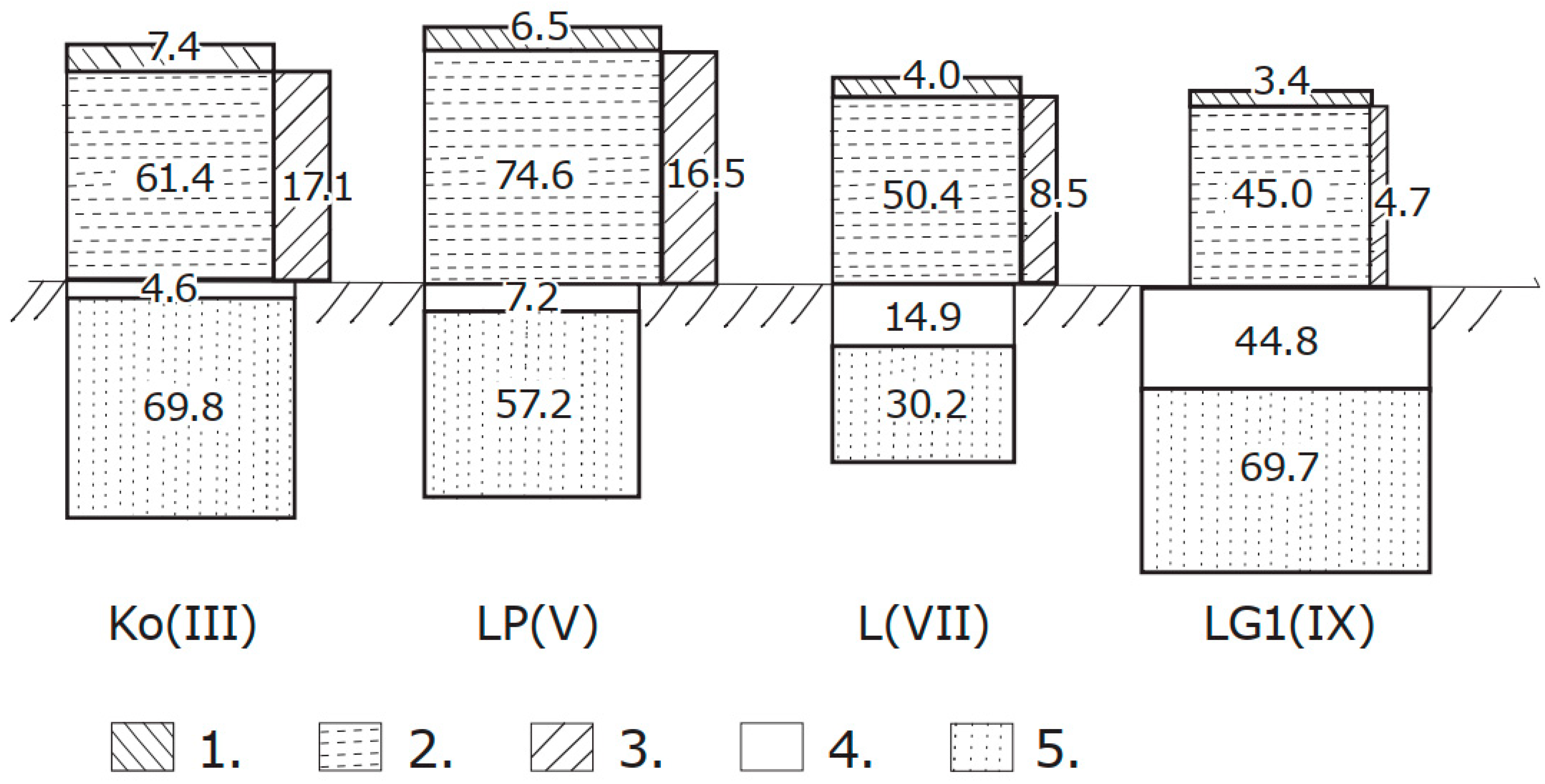
The graphical comparison of OC sequestration capacities of ecosystems’ phytocoenosis constituents (stems, branches and foliage) and the different layers of soil cover (forest floor and mineral part of soil cover) of four soil species (Ko, LP, L and LG1) is presented in Figure 3. In ecosystems formed in fresh moisture conditions, there are greater amounts of OC located in the phytocoenosis; on wet soils, greater amounts of OC accumulate in the soil cover. In general, the aboveground is the main storage for hemiboreal mature forests [4]
The annual OC increase in aboveground compartments of phytocoenoses and their constituents’ structures differ substantially by soil types (Figure 4). The AI of OC reached between 1.7 (LG1) and 5.2 (Ko) Mg OC ha−1. The forming of a 10−1 Mg or 102 kg overstorey tree stem phytomass or consisting of its OC on leached soil is accompanied by the formation of a stand’s foliage, branches and ground vegetation of 1.31, 1.12 and 0.81 units, respectively. The generalized similar ratio (stems: foliage: branches: ground vegetation) for Pseudopodzolic soils is 1.0:1.1:0.9:0.4, but for typical and peaty Podzols, the ratio is 1.0:0.8:0.7:0.7 and 1.0:0.6:0.5:1.3, respectively. Therefore, the accumulation of one Mg of OC in aboveground stems accompanied by the accumulation of OC as a by-product (or in needed for normal growth parts) varies from 2.2 (L) to 3.2 (Ko) Mg. From the other aspect, the annual OC accumulation in tree stems forms from the total aboveground phytocoenosis OC AI by the soil species Ko, LP, L and LG1 and it is 24%, 30%, 26% and 34%, respectively.
4.3. General Lines of Carbon Balance in Forest Ecosystems and Its Structural Compartments
In order to understand the CO2 accumulation/emission balance at the current time in forest ecosystems, both (1) the forming of AI from atmospheric CO2 and its accumulation in the form of OC in phytocoenosis and (2) the emission of CO2 from the ecosystem in the course of autotrophic and heterotrophic respiration need to be studied. In the present work, only the first part of the annual OC balance, i.e., AI is described. Itis possible to estimate the fixed amounts of atmospheric CO2 in the phytocoenosis using AI. The autotrophic respiration of ecosystems depends not only on the newly synthesized OC amounts but also on the standing phytocoenosis’ phytomass and the eco-physiologic state of the plant–soil system [32,33,34]. Ecosystem respiration was not studied in the present study. The heterotrophic respiration is in firm correlation with the amounts of formed annual forest litter and the death of a certain amount of stand trees within one year [35]. Of course, heterotrophic respiration depends to a great extent on the biological activity of soil organisms or destructors of soil organic matter [20].
The general assumption describes that in mature forests, which are in steady state ecosystems, the total annual emission of CO2 is generally equal to its sequestration (as OC) in an ecosystem [33]. In the case of studied forest ecosystems, the annual CO2 binding into the phytomass and its emission should be in the range from 5–6 (on less fertile soils) to 11–13 Mg CO2 ha−1 year−1 (on more fertile soils). Therefore, the intensity of ecological functioning of forests can differ more than two-fold depending on soil type. Sequestrated for a long time in tree stems, annual CO2 amounts are dependent on soil type, ranging from 1.4 to 4.5 Mg CO2 ha−1. Therefore, the timber production intensity may differ more than three-fold depending on the ecosystem’s soil cover and phytocoenosis composition. It should be mentioned that part of the CO2 assimilated in phytocoenosis is taken from the air layer located under the forest canopy, which is remarkably richer in CO2 content as compared to the air above the forest canopy [1,5]. Therefore, it refers to the recycling of carbon inside of forest ecosystems.
In a steady state ecosystem`s, its soil covers’ OC balance (input/output in Mg ha−1 year−1) is approximately equal. As a rule, the amounts of OC that have reached from the AI of phytocoenosis into the soil are always to a certain extent lower than their maximum, because parts of them have been mineralized without being separated from plants [35]. Amounts of CO2 that have accumulated into the soil cover vary in studied soils from 104 to 350 Mg CO2 ha−1. Thus, the greatest amounts are characteristic of wet and peaty soils, reaching 266–350 Mg CO2 per hectare. However, the CO2 amounts in fresh and moist soils, ranging in limits of 104–222 Mg CO2 ha−1, depend first and foremost on soil calcareousness [19,32]. Besides soil cover, certain amounts of OC are also located in the parent material, i.e., in the soil layer from the soil cover`s lower border to a depth of 1 m, but these OC amounts do not participate in the ecosystem’s active turnover.
4.4. OC Amounts in Belowground Phytomass and Their Annual Increase
The belowground phytomasses (stumps, large and fine roots, excluding the very fine ones), shown in Table 6, were estimated by linear models and calculated separately for spruce (n = 27, r = 0.89), pine (n = 33, r = 0.79 and birch (n = 24, r = 0.78) on the basis of previously published scientific literature data [19]. The belowground part of overstorey tree layer phytomass and the OC amounts within it were calculated after the amounts in aboveground woody parts (overstorey tree layer stems and branches). With these indirectly estimated OC amounts in tree layers and ground vegetation with underwood, it is possible to ascertain that in belowground forest phytocoenosis phytomass and its AI have been accumulated to 8.64 ± 1.82 and 0.54 ± 0.22 Mg OC ha−1, respectively. These calculations reveal that the total densities of OC in the whole phytocoenosis are by soil groups and in the range between 58 and 110 Mg OC ha−1 and its AI is between 2.4–6.2 Mg OC ha−1 year−1. Therefore, the mean share of OC in belowground phytomass and in its AI forms is 10.7 and 12.0%, respectively, of their amounts in the total phytocoenosis. The highest amounts of above- and belowground OC sum (>88 Mg OC ha−1) have been accumulated into phytocoenoses growing on pseudopodzolic, leached and eluviated soils and their gleyed versions. The lowest accumulation of OC (<67 Mg OC ha−1) is characteristic to Histic and Gleyed Podzols, and to dry skeletic rendzinas. Approximately the same kind of regularity is a characteristic of the AI of forests growing on the same soil types. On more fertile (leached, eluvic and pseudopodzolic) soils with their gleyed and gley versions formed phytocoenoses, the AI of OC per one hectare exceeds 6.2 Mg, but on podzolized sandy soils, the OC annual increment is under 3.0 Mg ha−1 year−1.
It is interesting to mention that despite the different pedo-ecological conditions, the OC sequestration rates have generally similar magnitude. According to Kumar et al. [36], the storage of OC in the 0–30 cm soil layer of the Himalayas Uttarakhand forest soils varies depending on altitude from 63 ± 5.9 (altitude a.s.l < 1000 m) to 105 ± 9.1 (>2000 m) Mg OC ha−1. However, the forest phytomass OC densities formed on these soils are dependent on forest species, ranging from 68 ± 11.5 (Pinus roxburghii) to 128 ± 11.5 (Abies pindrow) Mg OC ha−1.
According to Ostonen et al. [37], the critical phytomass of absorptive roots per stand basal area for transition of the foraging strategy is approximately 20 kg of absorptive roots per m2, despite the difference in absolute root nitrogen values. Based on these data, it may be concluded that the superficial density of fine roots in most studied ecosystems ranges from 0.51 to 0.62 Mg ha−1, which is approximately 0.26–0.31 Mg OC ha−1. It reveals that their share is greater in nitrogen-poor soils as compared to better growing conditions. This situation is also reflected by the C:N ratios, shown in Table 3. As a result of intensive cycling fine roots (2–3-fold during vegetation period), their share in AI is remarkably substantial.
Finally, the determined and developed on Estonian mineral soils forest ecosystems’ AI and its structure agree with the data presented by Jarvis et al. [38] on the characterization of the productivity of the boreal belt’s forest ecosystems. In addition to this, we would like to emphasize that in the AI levels of forest ecosystems, substantial differences dependent on soil type exist. Therefore, in research on forest ecosystems’ productivity (or AI), the soil types should be taken into account.
5. Conclusions
The highest total OC densities (>79 Mg OC ha−1) and annual increases (>4.8 Mg OC ha−1 year−1) of aboveground forest phytocoenoses were observed in pseudopodzolic soils (soil group V), formed from calcareous parent material on weak acid soils (groups III, IV and VIII) with a loamy texture, fresh to wet moisture conditions and a thin forest floor. The lowest total OC densities (<59 Mg OC ha−1) and annual increases (<2.8 Mg OC ha−1 year−1) of aboveground forest phytocoenoses were observed on strong acid sandy soils (groups VII and IX) with moist to wet moisture conditions and a thick forest floor. Depending on soil forest growing (site) conditions, the accumulated into mature coniferous forests’ tree stems OC stocks and aboveground annual increases range from 37 to 76 Mg OC ha−1 and from 0.7 to 1.9 Mg OC ha−1 year−1, respectively, whereas these amounts form from 70 to 81% and from 22 to 33% of their quantities in the whole phytocoenosis, respectively. On the basis of scientific literature, the data generalized by us allows us to conclude that the accumulated underground part of the phytocoenosis OC forms an average of 10.7% of its aboveground total amounts and 12.0% of its aboveground total AI. The OC surface densities varied on a great scale among the mineral soils; therefore, soil types should be taken into account for more precise reporting of forest ecosystem OC stocks.
Author Contributions
Conceptualization, R.K.; methodology, R.K.; statistical analysis, K.K.; writing—original draft preparation, R.K.; writing—review and editing, R.K., K.K., T.T. and R.L. All authors have read and agreed to the published version of the manuscript.
Funding
This research was funded by Estonian Research Council Grants No 4991, PSG730 and the programme Mobilitas Pluss (MOBTP168); by the European Regional Development Fund; by the European Commission’s Horizon 2020 programme under grant agreement no. 101000406 (project ONEforest); by target-financed projects of Estonian University of Life Sciences 0170116AGML98 and SF0172613AGML03.
Institutional Review Board Statement
Not applicable.
Informed Consent Statement
Not applicable.
Data Availability Statement
Data are available upon request from the corresponding author.
Acknowledgments
Many thanks to the colleagues from Soil Science of EULS and to Alar Astover.
Conflicts of Interest
The authors declare no conflict of interest.
References
- Ilvesniemi, H.; Forsius, M.; Finér, L.; Holmberg, M.; Kareinen, T.; Lepistö, A.; Piirainen, S.; Pumpanen, J.; Rankinen, K.; Starr, M.; et al. Carbon and nitrogen storages and fluxes in Finnish forest eco-systems. In Understanding the Global Systems; Käyhkö, J., Talve, L., Eds.; The Finnish Perspective: Turku, Finland, 2002; pp. 69–82. [Google Scholar]
- Pan, Y.; Birdsey, R.A.; Fang, J.; Houghton, R.; Kauppi, P.E.; Kurz, W.A.; Phillips, O.L.; Shvidenko, A.; Lewis, S.L.; Canadell, J.G.; et al. A large and persistent carbon sink in the world’s forests. Science 2011, 333, 988–993. [Google Scholar] [CrossRef] [PubMed] [Green Version]
- Lutter, R.; Kõlli, R.; Tullus, A.; Tullus, H. Ecosystem carbon stocks of Estonian premature and mature managed forests: Effects of site conditions and overstorey tree species. Eur. J. For. Res. 2019, 138, 125–142. [Google Scholar] [CrossRef]
- Ķēniņa, L.; Elferts, D.; Bāders, E.; Jansons, Ā. Carbon Pools in a Hemiboreal Over-Mature Norway Spruce Stands. Forests 2018, 9, 435. [Google Scholar] [CrossRef] [Green Version]
- Kleja, D.B.; Svensson, M.; Majdi, H.; Jansson, P.-E.; Langvall, O.; Bergkvist, B.; Johansson, M.-B.; Weslien, P.; Truusb, L.; Lindroth, A.; et al. Pools and fluxes of carbon in three Norway spruce ecosystems along a climatic gradient in Sweden. Biogeochemistry 2008, 89, 7–25. [Google Scholar] [CrossRef]
- Uri, V.; Varik, M.; Aosaar, J.; Kanal, A.; Kukumägi, M.; Lõhmus, K. Biomass production and carbon sequestration in a fertile silver birch (Betula pendula Roth) forest chronosequence. For. Ecol. Manag. 2012, 267, 117–126. [Google Scholar] [CrossRef]
- Grüneberg, E.; Ziche, D.; Wellbrock, N. Organic carbon stocks and sequestration rates of forest soils of Germany. Glob. Chang. Biol. 2014, 20, 2644–2662. [Google Scholar] [CrossRef]
- Wiesmeier, M.; Urbanski, L.; Hobley, E.; Lang, B.; von Lützow, M.; Marin-Spiotta, E.; van Wesemael, B.; Rabot, E.; Ließ, M.; Garcia Franco, N.; et al. Soil organic carbon storage as a key function of soils—A review of drivers and indicators at various scales. Geoderma 2019, 333, 149–162. [Google Scholar] [CrossRef]
- Giberti, G.S.; Wellstein, C.; Giovannelli, A.; Bielak, K.; Uhl, E.; Aguirre-Ráquira, W.; Giammarchi, F.; Tonon, G. Annual Carbon Sequestration Patterns in Trees: A Case Study from Scots Pine Monospecific Stands and Mixed Stands with Sessile Oak in Central Poland. Forests 2022, 13, 582. [Google Scholar] [CrossRef]
- Köster, T.; Kõlli, R. Interrelationships between soil cover and plant cover depending on land use. Est. J. Earth Sci. 2013, 62, 93–112. [Google Scholar]
- Högberg, P.; Wellbrock, N.; Högberg, M.N.; Mikaelsson, H.; Stendahl, J. Large differences in plant nitrogen supply in German and Swedish forests—Implications for management. For. Ecol. Manag. 2021, 482, 118899. [Google Scholar] [CrossRef]
- Bronick, C.J.; Lal, R. Soil structure and management: A review. Geoderma 2005, 124, 3–22. [Google Scholar] [CrossRef]
- Kõlli, R.; Köster, T. Interrelationships of humus cover (pro humus form) with soil cover and plant cover: Humus form as transitional space between soil and plant. Appl. Soil Ecol. 2018, 123, 451–454. [Google Scholar] [CrossRef]
- Morais, T.G.; Teixeira, R.F.; Domingos, T. Detailed global modelling of soil organic carbon in cropland, grassland and forest soils. PLoS ONE 2019, 14, e0222604. [Google Scholar] [CrossRef] [Green Version]
- Reintam, L. Taim-muld süsteem on elu alus [Plant-soil system is fundamentaal for life]. In Muld Ökosüsteemis, Seire ja Kaitse; Reintam, L., Ed.; ETA Looduskaitse Komisjon: Tartu, Estonia, 2004; pp. 11–23. [Google Scholar]
- Guo, L.B.; Gifford, R.M. Soil carbon stocks and land use change: A meta-analysis. Glob. Chang. Biol. 2002, 8, 345–360. [Google Scholar] [CrossRef]
- Hansson, K.; Olsson, B.A.; Olsson, M.; Johansson, U.; Kleja, D.B. Differences in soil properties in adjacent stands of Scots pine, Norway spruce and silver birch in SW Sweden. For. Ecol. Manag. 2011, 262, 522–530. [Google Scholar] [CrossRef]
- Zanella, A.; Jabiol, B.; Ponge, J.-F.; Sartori, G.; DeWaal, R.; Van Delft, B.; Graefe, U.; Cools, N.; Katzensteiner, K.; Hager, H.; et al. A European morpho-functional classification of humus forms. Geoderma 2011, 164, 138–145. [Google Scholar] [CrossRef] [Green Version]
- Kõlli, R.; Tamm, I. Humus cover and its fabric depending on pedo-ecological conditions and land-use: An Estonian ap-proach to classification of humus forms. Estonian J. Ecol. 2013, 62, 6–23. [Google Scholar] [CrossRef] [Green Version]
- Karlberg, L.; Gustafsson, D.; Jansson, P.-E. Modeling Carbon Turnover in Five Terrestrial Ecosystems in the Boreal Zone Using Multiple Criteria of Acceptance. Ambio 2006, 35, 448–458. [Google Scholar] [CrossRef]
- Stefańska-Krzaczek, E.; Szymura, T.H. Species diversity of forest floor vegetation in age gradient of managed scots pine stands. Balt. For. 2015, 21, 233–243. [Google Scholar]
- Lõhmus, E. Eesti Metsakasvukohatüübid (Estonian Forest Site Types); Eesti Loodusfoto: Tartu, Estonia, 2004. (In Estonian) [Google Scholar]
- Astover, A.; Reintam, E.; Leedu, E.; Kõlli, R. Muldade Väliuurimine [Survey of Soils]; Eesti Loodusfoto: Tartu, Estonia, 2013. (In Estonian) [Google Scholar]
- IUSS Working Group WRB. World Reference Base for Soil Resources 2014, Update 2015. International Soil Classification System for Naming Soils and Creating Legends for Soil Maps; World Soil Resources Reports No. 106; FAO: Rome, Italy, 2015. [Google Scholar]
- Whittaker, R.H. Branch dimensions and estimation of branch production. Ecology 1965, 46, 365–370. [Google Scholar] [CrossRef]
- Newbold, P.I. Methods for estimating net primary of forests. In IBP Handbook Nr 2; Willmer Brothers Limited Birkenhead: Birkenhead, UK, 1967; p. 29. [Google Scholar]
- Rodin, L.E.; Remezov, N.P.; Bazilevich, N.I. Metodicheskie Ukazanija k Izutšeniju Dinamiki i Biologitšeskovo Krugovorota Fitotsenozah; Leningrad, Russia, 1968; p. 143. (In Russian) [Google Scholar]
- Kachinsky, N. Fizica Pochvy [Soil Physics]; University Press: Moscow, Russia, 1965; Volume I. (In Russian) [Google Scholar]
- Kiviste, A. Eesti riigimetsa puistute kõrguse, diameetri ja tagavara vanuseridade diferentsmudel 1984–1993. aasta metsakorralduse andmeil. Trans. Est. Agric. Univ. 1997, 189, 63–75, (In Estonian with English Summary). [Google Scholar]
- Clarke, N.; Gundersen, P.; Jönsson-Belyazid, U.; Kjønaas, O.J.; Persson, T.; Sigurdsson, B.D.; Stupak, I.; Vesterdal, L. Influence of different tree-harvesting intensities on forest soil carbon stocks in boreal and northern temperate forest ecosystems. For. Ecol. Manag. 2015, 351, 9–19. [Google Scholar] [CrossRef]
- Cremer, M.; Kern, N.V.; Prietzel, J. Soil organic carbon and nitrogen stocks under pure and mixed stands of European beech, Douglas fir and Norway spruce. For. Ecol. Manag. 2016, 367, 30–40. [Google Scholar] [CrossRef]
- Kõlli, R. Ökosüsteemide fütoproduktiivsuse pedoökoloogiline analüüs. I. Metsad. Agraarteadus. 1991, 2, 39–60, (In Estonian with English Summary). [Google Scholar]
- Uri, V.; Kukumägi, M.; Aosaar, J.; Varik, M.; Becker, H.; Aun, K.; Lõhmus, K.; Soosaar, K.; Astover, A.; Uri, M.; et al. The dynamics of the carbon storage and fluxes in Scots pine (Pinus sylvestris) chronosequence. Sci. Total Environ. 2022, 817, 152973. [Google Scholar] [CrossRef]
- Aitsam, V.; Sims, A.; Tolm, T.; Nikopensius, M.; Karu, H.; Raudsaar, M.; Valgepea, M.; Timmusk, T.; Pärt, E. Statistiline Mets: 20 aastat Statistilist Metsainventeerimist Eestis; Keskonnaagentuur: Tallinn, Estonia, 2019. (In Estonian) [Google Scholar]
- Bazilevich, N.I.; Titljanova, A.A. Biotic Turnover on Five Continents: Element Exchange Processes in Terrestrial Natural Ecosystems; Publishing House SB RAS: Novosibirsk, Russia, 2008. (In Russian) [Google Scholar]
- Kumar, A.; Kumar, M.; Pandey, R.; ZhiGuo, Y.; Cabral-Pinto, M. Forest soil nutrient stocks along altitudinal range of Uttarakhand Himalayas: An aid to Nature Based Climate Solutions. Catena 2021, 207, 105667. [Google Scholar] [CrossRef]
- Ostonen, I.; Truu, M.; Helmisaari, H.-S.; Lukac, M.; Borken, W.; Vanguelova, E.; Godbold, D.; Lõhmus, K.; Zang, U.; Tedersoo, L.; et al. Adaptive root foraging strategies along a boreal–temperate forest gradient. New Phytol. 2017, 215, 977–991. [Google Scholar] [CrossRef] [Green Version]
- Jarvis, P.G.; Saugier, B.; Schulze, E.-D. Productivity of Boreal Forests. In Terrestrial Global Productivity; Roy, J., Saugier, B., Mooney, H.A., Eds.; Academic Press: San Diego, CA, USA; San Francisco, CA, USA; New York, NY, USA; Boston, MA, USA; London, UK; Sydney, Australia; Tokio, Japan, 2001; pp. 211–244. [Google Scholar]
Figure 1.
Estonian postlithogenic mineral soils and their correlation with WRB taxa. Soil codes and soil species names (in brackets are the soil names given by WRB): Kh—Limestone rendzinas (Rendzic Leptosols); Kr—Pebble-rich rendzinas (Calcari-Skeletic Regosols); K—Pebble rendzinas (Calcaric Cambisols); Ko—Leached or typical brown soils (Mollic Cambisols); Kog—Gleyed typical brown soils (Gleyic Cambisols); KI—Eluviated (brown) soils (Cutanic Luvisols); KIg—Gleyed eluvial soils (Gleyic Luvisols); LP—Pseudopodzolic soils (Glossic Retisols); Lk—Sod-podzolic soils (Umbric Podzols); Lkg—Gleyed sod-podzolic soils (Gleyic Umbric Podzols); L—Typical Podzols (Haplic Podzols); Lg—Gleyed Podzols (Gleyic Haplic Podzols); Go—Leached gley-soils (Mollic Gleysols); G(o)—Saturated gley-soils (Calcic Gleysols); GI—Eluviated gley-soils (Dystric Gleysols); LkG—Sod-podzolic gley-soils (Umbric Gleysols); LG—Gley-Podzols (Epigleyic Podzols); LG1—Peaty Podzols (Fibrihistic Podzols).

Figure 2.
Location of studied soil groups on a mineral soils’ matrix table. The O indicates the positions of the soil groups on the matrix table; on right side are the standard deviations of soil group mean positions by moisture (Hydr) and litho-genetic (Lt-Gn) scalars.
Figure 2.
Location of studied soil groups on a mineral soils’ matrix table. The O indicates the positions of the soil groups on the matrix table; on right side are the standard deviations of soil group mean positions by moisture (Hydr) and litho-genetic (Lt-Gn) scalars.

Figure 3.
Graphical comparison of organic carbon sequestration capacities of four different types of forest ecosystems, in Mg OC ha−1. The studied ecosystems are Ko(III), LP(V), L(VII) and LG1(IX), respectively, with soil code and soil group number (in brackets); compartments of ecosystems 1—foliage of tree layer, 2—stems of tree layer, 3—branches of tree layer, 4—forest floor and 5—soil organic matter in mineral soil layers.

Figure 4.
Annual organic carbon increases of aboveground compartments of phytocoenoses, in 0.1 Mg OC ha−1 year−1. Studied phytocoenoses–Ko(III), LP(V), L(VII) and LG1(IX), respectively, soil code and group number (in brackets); compartments of phytocoenosis 1—foliage of tree layer, 2—branches of tree layer, 3—stems of tree layer, and 4—ground vegetation.


Table 1.
Properties of research areas (n = 147) of soil cover or solum.
| Characteristic | Code | Unit | Code (1) and Group Number of Soil | ||||||||
|---|---|---|---|---|---|---|---|---|---|---|---|
| Kh Kr | K | Ko Kog | KI KIg | LP | Lk Lkg | L Lg | Go GI | LkG LG LG1 | |||
| I | II | III | IV | V | VI | VII | VIII | IX | |||
| Thickness | h | cm | 27.7 a | 55.6 bc | 46.8 b | 70.0 c–e | 92.8 f | 74.8 e | 64.8 cd | 64.6 c–e | 75.5 de |
| Fine earth | FE | 102 Mg ha−1 | 25.9 a | 68.2 bc | 59.2 b | 103.3 de | 143.7 f | 115.9 e | 92.8 cd | 87.0 b–d | 95.7 cd |
| Clay | CL | 10 Mg ha−1 | 66 a | 151 ab | 192 bc | 300 de | 349 e | 257 cd | 66 a | 265 b–e | 87 a |
| Specific surface area | SSA | Index 105 | 295 ab | 353 a–d | 348 bc | 471 d | 465 d | 379 b–d | 120 e | 460 cd | 230 a |
| Exchangeable acidity | EA | kmol ha−1 | 0.1 a | 0.2 a | 0.2 a | 7.6 a | 116 c | 71.8 b | 55.2 b | 4.5 a | 145 d |
| Hydrolytic acidity | HA | kmol ha−1 | 51 a | 122 ab | 114 a | 289 a–c | 543 c | 439 bc | 276 ab | 273 a–c | 762 e |
| Basic cations | BC | kmol ha−1 | 629 a–c | 1796 f | 1317 de | 1326 d–f | 1133 cd | 686 b | 300 a | 1894 f | 422 ab |
| Cation exchange capacity | CEC | kmol ha−1 | 680 ab | 1918 de | 1431 cd | 1615 de | 1676 de | 1124 bc | 576 a | 2170 e | 1246 cd |
| % of saturation | BS | % | 92.5 f | 93.0 ef | 90.0 ef | 80.6 de | 61.8 c | 58.4 c | 45.5 b | 76.1 d | 35.1 a |
| Soil organic matter | SOM | Mg ha−1 | 181 c | 194 cd | 134 ab | 165 bc | 111 a | 120 a | 78 e | 248 d | 202 c |
| Total nitrogen | NT | Mg ha−1 | 5.1 bc | 5.6 bc | 5.3 c | 6.5 c | 4.5 b | 4.9 b | 2.0 a | 10.8 d | 5.1 bc |
| SOC/NT | C/N | Index | 19.5 bc | 16.7 ab | 15.2 ab | 16.1 ab | 16.0 ab | 14.2 a | 24.1 d | 14.6 ab | 23.2 cd |
(1) For soil name, see Figure 1; Different lowercase letters within rows indicate a significant (p < 0.05) difference between soil groups.
Table 2.
Results of research areas’ stand taxation (inventory) (n = 193).
| Characteristic | Abbreviation | Unit | Code (1) and Group Number of Soil | ||||||||
|---|---|---|---|---|---|---|---|---|---|---|---|
| Kh Kr | K | Ko Kog | KI KIg | LP | Lk Lkg | L Lg | Go GI | LkG LG LG1 | |||
| I | II | III | IV | V | VI | VII | VIII | IX | |||
| Age | A | year | 98.9 b | 97.2 b | 89.7 b | 63.8 a | 79.5 ab | 80.1 ab | 78.4 ab | 80.9 ab | 84.9 b |
| Basal area (2) | BAbh | m2 ha−1 | 20.8 a | 20.3 a | 26.4 b | 27.3 bc | 30.8 c | 27.7 b | 27.1 b | 25.6 ab | 26.0 b |
| Stocking level | Stc lv | cf | 0.60 a | 0.58 a | 0.76 bc | 0.76 bc | 0.84 c | 0.78 bc | 0.78 bc | 0.73 a–c | 0.75 b |
| Stock of stem | Stc st | m3 ha−1 | 204 a | 225 ab | 291 bc | 312 bc | 390 d | 330 c | 271 b | 293 bc | 260 ab |
| % of spruce | Sp | % | 74.3 c | 44.8 bc | 71.1 c | 62.0 c | 65.2 c | 43.4 b | 5.9 a | 25.6 ab | 15.4 a |
| % of pine | Pn | % | 23.9 a–c | 33.7 bc | 9.8 ab | 0.6 a | 15.3 a–c | 28.4 c | 87.1 d | 11.1 a–c | 75.8 d |
| % of birch | Br | % | 1.1 a | 12.2 a-d | 10.1 ab | 26.0 cd | 17.8 b–d | 17.1 bc | 5.0 c | 32.0 d | 8.2 ab |
| Quality class | Q cl | class | IV,8 | II,4 | II,9 | I,6 | I,4 | I,3 | II,6 | I,1 | II,1 |
| Position of soil group on matrix’s hydro-scalar | 8.1 a | 16.3 ab | 18.0 b | 26.2 c | 25.2 c | 29.0 c | 20.7 b | 45.0 d | 51.0 d | ||
| Position of soil group on matrix’s litho-genetic scalar | 9.9 a | 14.8 b | 24.9 c | 35.2 e | 45.0 f | 53.7 g | 74.9 h | 30.8 d | 67.4 i | ||
(1) For soil name, see Figure 1; (2) Basal area at breast height; Different lowercase letters within rows indicate a significant (p < 0.05) difference between soil groups.
Table 3.
Areal densities of organic carbon (10−1 Mg OC ha−1) in aboveground phytomass (PM) and soil cover of different forest ecosystems’ types.
Table 3.
Areal densities of organic carbon (10−1 Mg OC ha−1) in aboveground phytomass (PM) and soil cover of different forest ecosystems’ types.
| Constituents (1) | Code (2) and Group Number of Soils | |||||||||
|---|---|---|---|---|---|---|---|---|---|---|
| Kh Kr | K | Ko Kog | KI KIg | LP | Lk Lkg | L Lg | Go GI | LkG LG LG1 | ||
| Name | Code | I | II | III | IV | V | VI | VII | VIII | IX |
| Herbs | Hrb | 2.63 bc | 3.92 e | 2.97 de | 3.41 de | 1.74 b | 1.98 bc | 0.54 a | 3.19 de | 0.28 a |
| Mosses | Mss | 6.76 a | 5.16 a | 6.62 a | 4.85 a | 5.72 a | 7.18 a | 18.64 b | 3.87 a | 21.62 c |
| Shrubs | Shr | 0.18 ab | 0.33 ab | 0.27 a | 0.06 a | 0.96 ab | 1.59 b | 3.67 c | 0.28 ab | 6.32 d |
| Ground vegetation | Grv | 9.6 a | 9.4 a | 9.9 a | 8.3 a | 8.4 a | 10.8 b | 22.8 b | 7.3 a | 28.2 c |
| Understorey trees | Unw | 7.4 a–c | 6.0 ab | 12.7 c | 18.6 d | 6.6 b | 4.8 ab | 3.1 a | 8.0 bc | 5.7 ab |
| Foliage of trees | Tre gr | 42.5 c | 33.6 bc | 60.6 d | 56.4 d | 57.8 d | n.d. (3) | 21.2 ab | 45.8 cd | 13.8 a |
| Branches of trees | Tre br | 99 b | 93 b | 150 c | 139 c | 156 c | n.d. | 68 b | 163 c | 35 a |
| Stems of trees | Tre st | 371 a | 442 ab | 596 bc | 566 bc | 762 d | n.d. | 475 d | 752 cd | 500 ab |
| Phytocoenosis | Phc tot | 529 a | 586 ab | 834 c | 789 bc | 1001 d | n.d. | 593 a | 917 cd | 518 a |
| -its green parts (4) | Phc gr | 51 a | 43 a | 72 c | 66 bc | 65 bc | n.d. | 38 a | 52 ab | 35 a |
| -its woody parts (5) | Phc wd | 107 b | 99 ab | 164 c | 158 c | 165 c | n.d. | 80 ab | 166 c | 58 a |
| OC in soil cover | SOC | 944 cd | 931 b–d | 765 bc | 954 cd | 644 b | 681 b | 445 a | 1503 e | 1139 d |
| From it in forest floor | SOC | 73 ab | 79 ab | 47 a | 48 a | 72 a | 110 ab | 158 b | 98 ab | 385 c |
(1) The total count of research areas (RA) for the determination PM of Grv and Unw was 193; for various tree layer parts and total phytocoenoses, it was 76. (2) For soil names, see Figure 1; (3) n.d.—not determined; (4) Foliage of trees together with green parts of understorey layers; (5) Woody parts without tree stems; The different lowercase letters within the rows indicate a significant (p < 0.05) difference between soil groups.
Table 4.
Annual increases (AI) of organic carbon (10−1Mg OC ha−1 year−1) in different aboveground constituents of forest phytocoenoses.
Table 4.
Annual increases (AI) of organic carbon (10−1Mg OC ha−1 year−1) in different aboveground constituents of forest phytocoenoses.
| Constituents (1) | Code (2) and Group Number of Soils | |||||||||
|---|---|---|---|---|---|---|---|---|---|---|
| Kh Kr | K | Ko Kog | KI KIg | LP | Lk Lkg | L Lg | Go GI | LkG LG LG1 | ||
| Name | Code | I | II | III | IV | V | VI | VII | VIII | IX |
| Herbs | Hrb | 2.89 cd | 4.31 e | 3.27 de | 3.75 de | 1.91 b | 2.18 bc | 0.59 a | 3.51 de | 0.30 a |
| Mosses | Mss | 1.65 a | 1.22 a | 1.76 a | 1.37 a | 1.43 a | 1.79 a | 4.60 b | 0.96 a | 4.56 b |
| Shrubs | Shr | 0.04 a | 0.10 ab | 0.07 a | 0.00 a | 0.31 a | 0.73 bc | 1.06 cd | 0.00 a | 1.44 d |
| Ground vegetation | Grv | 4.58 | 5.63 | 5.10 | 5.12 | 3.65 | 4.70 | 6.25 | 4.47 | 6.30 |
| Understorey trees | Unw | 1.03 ab | 1.37 a–c | 2.43 cd | 2.77 d | 1.46 b | 0.75 ab | 0.39 a | 0.64 ab | 0.49 a |
| Foliage of trees | Tre gr | 9.8 b | 8.9 ab | 15.6 c | 15.1 c | 15.7 c | n.d. (3) | 7.1 ab | 16.1 c | 4.7 a |
| Branches of trees | Tre br | 8.1 a | 7.1 a | 13.3 c | 12.6 c | 13.1 c | n.d. | 5.7 ab | 14.5 c | 3.3 b |
| Stems of trees | Tre st | 6.8 a | 6.9 a | 12.2 b | 17.0 cd | 14.5 bc | n.d. | 9.3 a | 19.2 d | 7.0 a |
| Phytocoenosis | Phc tot | 33.2 b | 29.6 ab | 48.3 c | 52.0 c | 47.8 c | n.d. | 27.8 ab | 54.8 c | 22.4 a |
| -its green parts (4) | Phc gr | 14.6 a | 14.9 ab | 21.5 c | 20.9 c | 19.7 c | n.d. | 12.3 a | 20.7 bc | 11.4 a |
| -its woody parts (5) | Phc wd | 8.6 b | 7.8 b | 15.1 c | 14.1 c | 13.9 c | n.d. | 6.1 ab | 14.9 c | 4.0 a |
(1) Total count of research areas (RA) for the determination of AI of Grv and Unw was 193, but for various tree layer parts and total phytocoenoses, it was 76; (2) For soil name, see Figure 1; (3) n.d.—not determined; (4) Foliage of trees together with green parts of understorey layers; (5) Woody parts without tree stems; Different lowercase letters within rows indicate a significant (p < 0.05) difference between soil groups.
Table 5.
The percentage of different constituents of phytocoenoses (Phc) in the total aboveground phytomass and in its annual increases (n = 76).
Table 5.
The percentage of different constituents of phytocoenoses (Phc) in the total aboveground phytomass and in its annual increases (n = 76).
| Characteristics | Constituents (1) | Code (2) and Group Number of Soils | |||||||
|---|---|---|---|---|---|---|---|---|---|
| Kh Kr | K | Ko Kog | KI KIg | LP | L Lg | Go GI | LkG LG LG1 | ||
| I | II | III | IV | V | VII | VIII | IX | ||
| Constituent % from Phc PMt | Hrb | 0.49 c | 0.81 d | 0.36 c | 0.40 c | 0.16 ab | 0.06 a | 0.31 bc | 0.04 a |
| Mss | 1.24 a | 0.84 a | 0.89 a | 0.71 a | 0.54 a | 4.15 b | 0.43 a | 5.42 c | |
| Unw | 1.53 ab | 1.54 ab | 1.64 ab | 2.65 b | 0.78 a | 0.75 a | 0.32 a | 1.89 ab | |
| Tre | 96.7 c | 96.6 bc | 96.7 c | 96.4 bc | 98.4 c | 94.4 b | 99.0 c | 89.7 a | |
| Consituent % from Phc AIt | Hrb | 7.92 d | 14.69 e | 6.33 d | 6.20 d | 3.10 bc | 1.11 a | 5.72 cd | 0.86 ab |
| Mss | 4.81 a | 4.06 a | 3.88 a | 2.71 a | 2.97 a | 15.96 b | 2.03 a | 27.60 c | |
| Unw | 3.29 a–d | 5.32 b–d | 5.20 cd | 6.03 d | 3.34 a–c | 1.35 a | 1.15 ab | 2.85 a-d | |
| Tre | 76.8 b | 75.6 b | 84.5 bc | 85.1 bc | 89.9 c | 78.4 b | 91.2 c | 61.6 a | |
| % green parts | in Phc PMt | 9.66 d | 7.84 b–d | 8.69 cd | 8.48 cd | 6.63 ab | 6.72 ab | 5.40 a | 7.73 bc |
| in Phc AIt | 45.2 a–c | 51.1 cd | 44.5 ab | 40.4 ab | 40.8 a | 45.3 b | 40.4 ab | 53.6 d | |
| % stand stems | in Phc PMt | 70.0 a | 74.6 ab | 71.5 a | 71.4 a | 76.6 bc | 79.6 c | 77.5 bc | 80.7 c |
| in Phc AIt | 21.8 a | 22.8 ab | 25.6 a–c | 31.8 cd | 30.8 d | 33.2 d | 31.3 b–d | 29.5 b–d | |
| % AI from Phc PMt | AIt/PMt | 6.39 bc | 5.32 ab | 5.83 bc | 6.70 c | 4.91 a | 4.88 a | 5.65 a–c | 4.42 c |
| % forest floor OC from total soil cover OC | 7.7 | 8.5 | 6.1 | 5.0 | 11.2 | 35.5 | 6.5 | 33.8 | |
| Ratio: Soil cover OC/Pch OC | 1.8 | 1.6 | 0.9 | 1.2 | 0.6 | 0.7 | 1.6 | 2.2 | |
Table 6.
Estimations of organic carbon in belowground phytomass (Mg ha−1) and in its AI (Mg ha−1 year−1) for studied soil groups [19].
Table 6.
Estimations of organic carbon in belowground phytomass (Mg ha−1) and in its AI (Mg ha−1 year−1) for studied soil groups [19].
| Soil Group | OC Density, 10−1 Mg ha−1 | AI, 10−1 Mg ha−1 year−1 | |||||||
|---|---|---|---|---|---|---|---|---|---|
| Code | No | Bgr (1) Gv + Uw | Bgr (2) Tr Woody | Bgr (3) PM | Phc (4) PM Sum | Bgr Gv + Uw | Bgr Tr woody | Bgr AI | Phc AI Sum |
| Kh Kr | I | 6.7 | 71.0 | 77.8 | 607 | 3.1 | 2.2 | 5.3 | 38.6 |
| K | II | 9.2 | 75.6 | 84.8 | 671 | 4.6 | 2.0 | 6.6 | 36.2 |
| Ko Kog | III | 8.2 | 105.1 | 113.3 | 947 | 3.7 | 3.6 | 7.3 | 55.6 |
| KI KIg | IV | 9.6 | 84.5 | 94.2 | 883 | 4.2 | 3.5 | 7.7 | 59.7 |
| LP | V | 5.2 | 92.0 | 97.2 | 1098 | 2.3 | 2.8 | 5.1 | 52.9 |
| Lk Lkg | VI | 5.5 | n.d. (5) | n.d. | n.d. | 2.6 | n.d. | n.d. | n.d. |
| L Lg | VII | 2.6 | 59.8 | 62.4 | 655 | 0.9 | 1.7 | 2.5 | 30.3 |
| Go GI | VIII | 8.0 | 91.5 | 99.5 | 1016 | 3.6 | 3.4 | 7.0 | 61.8 |
| LkG LG LG1 | IX | 3.0 | 58.8 | 61.8 | 580 | 0.6 | 1.1 | 1.7 | 24.1 |
| Mean | 6.5 | 79.8 | 86.4 | 807 | 2.8 | 2.5 | 5.4 | 44.9 | |
| STdev | 2.6 | 16.4 | 18.2 | 203 | 1.4 | 0.9 | 2.2 | 14.4 | |
(1) Belowground parts of ground vegetation and understorey trees; (2) Belowground woody parts of tree layers; (3) Total belowground phytomass; (4) Total phytomass of phytocoenosis; (5) n.d.—not determined.
Publisher’s Note: MDPI stays neutral with regard to jurisdictional claims in published maps and institutional affiliations. |
© 2022 by the authors. Licensee MDPI, Basel, Switzerland. This article is an open access article distributed under the terms and conditions of the Creative Commons Attribution (CC BY) license (https://creativecommons.org/licenses/by/4.0/).
Share and Cite
MDPI and ACS Style
Kõlli, R.; Kauer, K.; Tõnutare, T.; Lutter, R. Ecosystem Carbon Stocks and Their Annual Sequestration Rate in Mature Forest Stands on the Mineral Soils of Estonia. Forests 2022, 13, 784. https://0-doi-org.brum.beds.ac.uk/10.3390/f13050784
AMA Style
Kõlli R, Kauer K, Tõnutare T, Lutter R. Ecosystem Carbon Stocks and Their Annual Sequestration Rate in Mature Forest Stands on the Mineral Soils of Estonia. Forests. 2022; 13(5):784. https://0-doi-org.brum.beds.ac.uk/10.3390/f13050784
Chicago/Turabian StyleKõlli, Raimo, Karin Kauer, Tõnu Tõnutare, and Reimo Lutter. 2022. "Ecosystem Carbon Stocks and Their Annual Sequestration Rate in Mature Forest Stands on the Mineral Soils of Estonia" Forests 13, no. 5: 784. https://0-doi-org.brum.beds.ac.uk/10.3390/f13050784
Note that from the first issue of 2016, this journal uses article numbers instead of page numbers. See further details here.