Comparison of Variable Selection Methods among Dominant Tree Species in Different Regions on Forest Stock Volume Estimation

Abstract

The forest stock volume (FSV) is one of the crucial indicators to reflect the quality of forest resources. Variable selection methods are usually used for FSV estimated models. However, few studies have explored which variable selection methods can make the selected data set have better explanatory and robustness for the same dominant tree species in different regions after the feature variables were filtered by the feature selection methods. In this study, we chose six dominant tree species from Lin’an District, Anji County, and a part of Longquan City. The tree species include broad-leaved, coniferous, Masson pine, Chinese fir, coniferous and broad-leaved mixed forest, and all tree species which include the above five groups of tree species. The last two tree species were represented by mixed and all, respectively. Then, the satellite images, terrain factors, and forest inventory data were selected by six variable selection methods (least absolute shrinkage and selection operator (LASSO), recursive feature elimination (RFE), stepwise regression (Step-Reg), permutation importance (PI), mean decrease impurity (MDI), and SelectFromModel based on LightGBM (SFM)), according to different dominant tree types in different regions. The selected variables were formed into a new dataset divided by different dominant trees. Besides, extreme gradient boosting (XGBoost) was used, combined with variable selection methods to estimate the FSV. The performed results are as follows: In the feature selection of coniferous, RFE performed better both in the average and in the separate regions. In the feature selection of Chinese fir and all, PI performed better both in the average and in the separate regions. In the feature selection of Masson pine, MDI performed better both in the average and in the separate regions. In the feature selection of mixed, MDI performed better in the average while RFE performed better in the separate regions comprehensively. The results showed that not only in separate regions, but the average result two factors, RFE, MDI, and PI all performed well to select variables to estimate the FSV. Furthermore, we selected the top five high feature-importance factors of different tree types, and the results showed that tree age and canopy density were both of great importance to the estimation of FSV. Besides, in the exhibited results of feature selection methods, compared with no variable selection, the research also found that variable selection can improve the performance of the model. Additionally, from the results of different tree types in different regions, we also found that small-scale and diversity of dominant tree types may lead to the instability and unreliability of experimental results. The study provides some insight into the application the optimal variable selection methods of the same dominant tree type in different regions. This study will help the development of variable selection methods to estimate FSV.

1. Introduction

Forests are a vital ecosystem on the earth which play an important role in the global carbon cycle and provide habitats for a wide diversity of wild fauna and flora [1]. The forest stock volume (FSV, m³/mu, 1 mu = 0.06667 ha), which is defined as the sum of the stem volumes of all living trees per unit area [2], is one of the key indicators for forest resource assessment. Due to various types of human activities leading to changes in carbon stocks, FSV data need to be updated regularly [3]. Traditionally, financial and logistical constraints may lead to low quality of field measurements of the FSV [4]. With the development of remote sensing technology, currently an effective rapid estimation method has been performed to estimate the forest FSV, which combined remote sensing images and plot data.

Remote sensing data has been widely used in various studies. Lindberg et al. [5] compared estimation of forest variables from regression models based on measures derived from Airborne Laser Scanning (ALS) data in small (0.5 m) raster cells, based on variables derived from the 3D point cloud. Earlier in 2001, Tomppo et al. [6] proposed a multisource and multiresolution method, which combined Landsat TM data and IRS-1C WiFS data, together with field plot data from the National Forest Inventories (NFIs), to estimate a large area of growing stock. A study conducted by Gonzlez-Alonso et al. [7] found a highly dependent relationship between satellite data and ground information from forest surveys. In their research, Razi Ahmed et al. [8] thought that the ability of LiDAR remote sensing technology to cover large areas is a very useful tool for large-scale biomass estimation. Zhang et al. [9] used TM images, combined with topographic factors and forest characteristics factors, to predict the total forest accumulation in the Three Gorges Reservoir Region, and the overall prediction accuracy reached 89.58%. Besides, multispectral remote sensing images, combined with many other factors, are widely used as feature variables for forest accumulation prediction.

In the FSV, growing stock volume (GSV), or biomass estimation field, some studies have examined assessments through using remote sensing and regression model. Matteo Mura et al. [10] found that Sentinel-2A imagery performed well by utilizing eight k-nearest neighbors (kNN) methods to estimate the GSV of forest. In the study of Pang et al. [11], the accuracy of Sentinel-2A satellite image combined with kNN in three scales of forestry bureau, forest farm, and subclass reached 97.0%, 93.2%, and 83.6%, respectively. By using the stepwise regression-based multiple linear regression models, in the research of Li et al. [12], they found it achieved better than using Boruta-based multiple linear regression models. Four different machine-learning algorithms were used to build regression models by Li et al. [13] for aboveground biomass (AGB) estimation, and they found that the most powerful coefficients with the estimated AGB were the height and coverage variables of photogrammetric point cloud, texture mean value, and the visible differential vegetation index of the digital orthophoto mosaic. Li et al. [14] used Sentinel-2A imagery data, forest inventory data, and digital elevation model (DEM) data of the study area, and combined the Stacking model with LASSO in their study on the FSV estimation of Linhai City and Chun’an County, and the minimum MAPE of the FSV estimation reached 20.24%. To estimate the forest GSV in Georgia, Obata et al. [15] presented a random forest regression (RFR) model with 30 m spatial resolution, and they indicated that the ecophisiological variations in each forest performed better by the variables derive from Landsat time series.

In the FSV, GSV, or biomass estimation models, except for remote sensing spectrum, there are a variety of feature factors that can be used as candidate variables for FSV or ground biomass estimation [16,17,18,19]. The variables include vegetation indices, image texture characteristics, terrain factors and forest inventory data, etc. Using a large number of feature variables can increase the likelihood of improving the prediction model accuracy. However, it may increase computational load, data noise, or interference [20]. Besides, high-dimensional images often result in information redundancy and “dimension disasters” [21]. At this time, variable selection is a good method to improve efficiency and prediction accuracy. Variable selection methods are commonly used for prediction models [22] based on high-dimensional data. For example, Yu et al. [19] compared the performance among ten variable selection approaches based on linear regression model to estimate subtropical forest biomass. They found that the Bayesian criteria (BIC) method was the best result in comprehensive evaluation. Additionally, lots of researchers combinate variable selection approaches with machine learning algorithms to evaluate forest biomass and then select the better performance results from various models. Based on Landsat OLI data, Luo et al. [18] imputed the aboveground biomass of forest by using three variable selection methods and three machine learning algorithms. They put forward that combining RFE and CatBoost modeling to estimate the AGB is the best combination method. Li et al. [23] proposed an adaptive feature variable combination optimization (AFCO) program to estimate the GSV of coniferous plantations. They selected feature variables from three datasets (GF-2, Sentinel-2, and the integrated data) following the AFCO and four other variable selection methods, which combined with KNN or RFR to estimate the GSV. The result showed that the GSV estimation obtained by the AFCO method was more accurate, as the RMSErs were 30.0%, 23.7%, 17.7%, and 17.5% lower than four other feature selection methods, respectively. The above examples show the importance of variable selection method in predicting forest resources information. However, in different regions, owing to different terrain factors, weather, or other reasons, the factors strongly related to dominant tree types, which represent the largest proportion of tree species in the mixed forests, might change a lot. Few studies have explored which variable selection methods can make the selected data set have better explanatory and robustness for the same dominant tree species in different regions after the feature variables were filtered by the feature selection methods.

The data used in China’s forest field survey is mainly based on forest inventory data. During the FSV estimation, data of permanent plots (the basic units of NFI, set up by systematic sampling methods at the intersection of kilometer networks referring to the topographic maps with 1:50,000 map scale, usually with an area of 0.0667 ha) are frequently chosen to validate the prediction of FSV [24,25]. However, the number of subclasses (the basic unit of inventory for forest management planning and design, divided by the terrain boundaries, including ridge line, valleys, roads, etc., or forest ownership boundaries) is much larger than the number of permanent plots in China. To reduce the cost of investigating, the estimation of FSV based on subplots is more valuable than methods based on permanent forest plots.

In this paper, six variable selection methods were opted to combine with XGBoost, which is a regression model, to estimate the FSVs of six dominant tree species divided by three different areas in Zhejiang Province of China. The purposes of this study are as follows:

• Identifying which feature selection approaches have better performance on the same type of tree species in different regions.
• Exploring whether feature selection method is more effective in estimating the FSV than without feature selection method. Additionally, from the estimated results, exploring which features were crucial to the FSV estimation.
• Exploring whether the small-scale and diversity of forest types will lead to the bad performance and exploring whether the amount is big enough that the above phenomenon would disappear.

2. Study Area

The experimental study areas were selected from three places in Zhejiang Province, include Anji County, Lin’an District, and a part of Longquan City (Figure 1). Each region has a multitude of dominant tree types. In order to explore different tree species in different regions as far as possible, we chose six species, which would be introduced in the next section.

Anji County is a Municipal County (1885.71 km², 30°23′–30°53′ N, 119°14′–119°53′ E) of Huzhou City, Zhejiang Province. It belongs to the north subtropical monsoon climate zone. The main vegetation types in the territory include subtropical coniferous forest, evergreen broad-leaved forest, subtropical coniferous and broad-leaved mixed forest, and subtropical bamboo forest. Anji has a forest area of 138,227.72 hm², most of which are distributed in hills [26].

Lin’an District (3134.78 km², 29°56′–30°23′ N, 118°51′–119°52′ E) is located in the west of Hangzhou, Zhejiang Province and at the foot of southern Tianmu Mountain. It is about 100 km long from east to west and 50 km wide from north to south, with a total area of 312,600 hm². The forest vegetation in Lin’an District belongs to the subtropical evergreen broad-leaved forest distribution area. The vegetation types and flora of the whole region are complex, which can be divided into evergreen broad-leaved forest, coniferous broad-leaved mixed forest, coniferous forest, and so on.

Longquan City (3059 km², 27°42′–28°20′ N, 118°42′–119°25′ E) is located in the southwest of Zhejiang Province. It is 70.25 km wide from east to west and 70.80 km long from north to south, with a total area of 3059 km². The forest area reached 257,200 hm² and the volume reached 19.12 million m³ [16]. We chose an area in the southern Longquan City, and we used Longquan City or Longquan area to represent this area in the following text.

3. Data

The research data include forest inventory data, digital elevation model, and Sentinel-2A satellite data.

3.1. Forest Inventory Data

The research data come from the forest resource inventory data in Longquan City in 2016, Lin’an District in 2019 and Anji County in 2018, with subclass as the unit (

Table 1. Groups divided by the area and the dominant tree species and the number of subplots.

Area	Dominant Tree Species	Number of Subplot	Proportion (%)
	Broad-leaved	3027	36.88
	Coniferous	443	5.40
Anji County	Chinese Fir	1716	20.91
	Masson Pine	1808	22.03
	Mixed	1213	14.78
	All	8207	100
	Broad-leaved	13,785	34.32
	Coniferous	4439	11.05
Lin’an District	Chinese Fir	8846	22.03
	Masson Pine	7463	18.58
	Mixed	5630	14.02
	All	40,163	100
	Broad-leaved	101	1.75
	Coniferous	1656	28.63
A part of Longquan City	Chinese Fir	3086	53.34
	Masson Pine	154	2.66
	Mixed	788	13.62
	All	5785	100

). The dominant tree species, which mean the largest proportion tree species in all the mixed forests, were divided into broad-leaved, coniferous, Chinese fir, Masson pine, coniferous and broad-leaved mixed forest, and all tree species, which include the above five groups of tree species. The tested six groups of dominant tree species are expressed by broad-leaved, coniferous, Chinese fir, Masson pine, mixed, and all, respectively.

3.2. Characteristic Variable Extraction Based on Image Data

In this study, DEM (ASTER GDEM), with a spatial resolution of 30 m in Lin’an District, Longquan City, and Anji County, were obtained from the geographic data space Bureau, and elevation, slope, and aspect were extracted from the aster GDEM data as topographic factors.

The satellite imageries used in the study were downloaded from ESA (https://scihub.copernicus.eu/, accessed on 6 November 2021). The Sentinel-2A imageries, which have no clouds, were of good quality in the study area selected. Longquan City, Lin’an District, and Anji City images were acquired on 28 March 2016, 13 February 2019, and 1 October 2018, respectively. The imageries were from L1-level product, which is an atmospheric apparent reflectance product after orthorectification and sub-cell geometric precise correction [27], thus, only atmospheric correction was required. In this study, we used SNAP to resample the bands at the resolution between 20 m and 60 m to the resolution of 10 m through using the nearest neighbor method, then converted Envi standard format for clipping in Envi.

Eleven bands were extracted from the Sentinel-2A satellite imageries and 14 commonly used vegetation indices [14,28,29,30,31] were calculated. For forest variable prediction in the boreal forest, Astola et al. [28] found that the best predictive Sentinel-2 image band was the band5. In addition, according to related studies [29,30], the correlation between reflectance at 705 nm and chlorophyll content is better than that at 740 and 783 nm. Therefore, the band at 705 nm band5 is selected in this paper as the red-edge band in the calculation of vegetation index.

The paper used the gray level co-occurrence matrix method put forward by Haralick et al. [32], then used PCA to extract the first principal component. Besides, we chose eight GLCM texture features, which encompass Mean (ME), Variance (VA), Homogeneity (HO), Contrast (CO), Dissimilarity (DI), Entropy (EN), Second Moment (SM), and Correlation (CC), whose window sizes were 5 × 5.

3.3. Data Integration

In this article, the feature variables included 11 multispectral bands, 14 vegetation indices calculated based on bands, DEM, texture features, and forest inventory data, as shown in

Table 2. Summary of predictor variables, including Sentinel-2A spectral variables, vegetation indices, texture measures, and forest factors.

Variable Type	Characteristic Variable	Variable Number	Description
Spectral variable	Band2, Band3, Band4, Band5, Band6, Band7, Band8, Band8a, Band9, Band11, Band12	11	Sentinel-2A bands
Vegetation indices	NDVI EVI SR DVI SAVI CIgreen NDWI NDVIre SRre MTCI MCARI NDI45 MSRre CIre	14	(B8 − B4)/(B8 + B4) 2.5 × (B8 − B4)/(B8 + 6 × B4 − 7.5 × B2 + 1) B8/B4 B8 − B4 (B8 − B4)/(B8 + B4 + 0.5) × 1.5 B8/B3 − 1 (B3 − B5)/(B3 + B5) (B8 − B5)/(B8 + B5) B8/B5 (B8 − B5)/(B5 − B4) [(B5 − B4) − 0.2 × (B5 − B3)] × (B5 − B4) (B5 − B4)/(B5 + B4) (B8/B5 − 1)/$\sqrt{\frac{B8}{B5}+1}$ (B8/B5) − 1
Texture measures	Elevation, Slope, Aspect	3
Forest factors	Canopy density, Soil thickness, Tree age, Thickness of soil humus, Vegetation Coverage, Dominant Species	5

Note: BX represent BandX of Sentinel-2A.

below. Among them, the dominant tree species, which is a variable of forest inventory data, only have this feature for all tree species.

3.4. Data Preprocessing

(1)

Delete the missing value of the data set and eliminate the small class data with stock volume of 0.

(2)

Data normalization:

Due to the different value ranges among most attributes in the training set and test set of intrusion detection [33], and in order to make the data processing and model learning process more convenient and efficient, the training data was normalized and preprocessed so that the load value of the training data is between 0 and 1. The data normalization equation adopted in this paper is:

$$x_{norm}=\frac{x-x_{min}}{x_{max}-x_{min}}$$

(1)

4. Methods

4.1. Study Scheme Design

In this study, we adopted the strategy of cross validation. The overall purpose of cross validation is to select a model then use the complete data set to refit the selected model, so as to accurately evaluate the prediction error [34]. The commonly used methods of cross validation are LOOCV and K-fold cross-validation (K-fold CV). K-fold CV is to divide the data set into K subsets, then take one of the K subsets as the verification data set and the other K-1 data sets as the training set, calculate the K models, and take their average prediction accuracy as the final accuracy value. To compare the performance among different variable selection methods, Yu et al. [19] employed 50 times 10-fold cross validation in the linear regression model to estimate aboveground biomass. Huang et al. [16] combined stepwise regression and XGboost to estimate the FSV, and also used ten-fold cross validation in the training model. LOOCV mainly refers to the assumption that n is the number of samples in the training set, only one training sample is retained as the test set every time, and all the remaining samples are used as the training set training model. The prediction result of this method is more accurate, but its operation cost and time consumption are large. The test set in the model was used to test the accuracy of the training algorithm [35], and its performance showed the generalization ability of the network.

In this study, 10-fold cross validation method was employed in the train sets to optimize the model. We firstly selected the FSV of two of three regions as train set, one as test set. Then, the FSV train sets classified by six dominant tree species, as well as three regions, were randomly divided into ten sets, nine of which are used as train sets and one as test set. This process is repeated ten times to prevent the phenomenon of “over-fitting”. Then, the test set was used to evaluate the model.

For the three regions of the study, we took subclass as unit, and each area was divided according to six dominant tree types. We took two regions as the training set and the remaining one as the test set. In other words, three groups of experiments were required for the verification of each variable selection methods:

(1)

Training set: Lin’an District, Longquan City; Test set: Anji County

(2)

Training set: Lin’an District, Anji County; Test set: Longquan City

(3)

Training set: Longquan City, Anji County; Test set: Lin’an District.

Finally, we classified the results of the three test sets according to the dominant tree types and obtained the average value of their estimation results. Through the average value, we could observe the accuracy of the variable selection methods in selecting different dominant tree variables in different regions.

4.2. Formatting of Mathematical Components

As a data preprocessing process, variable selection plays an important role in data mining and machine learning. It could be considered that feature analysis is a process of designing feature collection for machine learning applications [36]. Through variable selection, the complexity of the problem can be reduced, and the prediction accuracy, robustness, and interpretability of the learning algorithm can be improved [37].

4.2.1. Least Absolute Shrinkage and Selection Operator Method

LASSO was proposed by Robert Tibshirani [37]. The main idea of LASSO is to use L1- regularization to generate sparse regression solution, that is, when constructing linear regression model, add penalty term to make the sum of regression coefficients less than a certain threshold, minimize the sum of squares of residuals, and compress the regression coefficients of some characteristic variables to 0, so as to achieve the purpose of dimensional reduction by deleting these variables. The larger the λ, the stronger the compression effect on the estimated parameters, and the fewer variables can be selected. The smaller the λ, the less the model variables, and the smaller the penalty in the model. The study used a 3-fold cross-validation. The equation of LASSO is generally expressed as follows:

$${\widehat{\beta }}^{LASSO}=\underset{\beta }{\mathrm{argmin}}\left\{\frac{1}{2}{{\displaystyle \sum }}_{i=1}^N{\left(y_i-{\beta }_0-{{\displaystyle \sum }}_{j=1}^p{x}_{ij}{\beta }_j\right)}^2+\lambda {{\displaystyle \sum }}_{j=1}^p\left|{\beta }_j\right|\right\},\lambda \in \left[0,\infty \right)$$

(2)

4.2.2. Recursive Feature Elimination

RFE is a packaging method for finding the optimal feature subset proposed by Guyon et al. [38] based on SVM. It is a model-based backward search method. The feature set at the beginning of the algorithm is all variables. In each subsequent iteration, the modeling is carried out according to the current feature set. After the modeling was completed, the feature with the lowest score was deleted according to the score of each feature, and the algorithm continues to iterate according to the above process until the feature subset is empty. This study adopts a 10-fold cross-validation method of RFE.

4.2.3. Stepwise Regression

Stepwise regression (Step-Reg) is also a packaging method in feature selection. It established the linear relationship between FSV and original variable set through multiple linear regression method. Step-Reg is the process of selecting a stepwise way for F-test [39] and gradually eliminating irrelevant factors. Only important variables are included in the final regression equation to ensure that the final set of explanatory variables is optimal.

We used SPSS for Step-Reg analysis. Generally, probability (p) has three values, 0.001, 0.01, and 0.05. It is considered statistically significant if it is 0.01 < p ≤ 0.05, and 0.001 ≤ p ≤ 0.01 is highly statistically significant. The evaluation factors of p ≤ 0.05 in this study were retained.

4.2.4. Permutation Importance

Breiman [40] thought that after each tree in the random forest was constructed, the importance of the features could be measured by randomly replacing the $m_{th}$ features. Let $X$ be the original eigenvalue matrix, $X^{\pi ,m}$ be a new matrix obtained by randomly replacing the $m_{th}$ column of the $X$ matrix, and $L\left(y_i,f\left(x_i\right)\right)$ be expressed as the loss function obtained by $f\left(x_i\right)$ to predict $y_i$, then the characteristic importance of $m_{th}$ can be expressed as follows:

$$V{I}_m^{\pi }={\displaystyle \sum }_{i=1}^{N}L\left(y_i,f\left(x_i^{\pi ,m}\right)\right)-L\left(y_i,f\left(x_i\right)\right)$$

(3)

In this paper, we used PI to represent Permutation Importance.

4.2.5. Mean Decrease Impurity

Random forest provides an algorithm of mean decrease impurity for feature selection. Mean decrease impurity determines the importance of the feature by calculating the reduction degree of the feature to the average value of node impure of all regression decision trees in the random forest. It uses Gini index to measure node impurity. The more Gini index decreases, the more node impurity decreases, so this feature is more important. Gini index is calculated as follows:

$$G{I}_m={\displaystyle \sum }_{k=1}^{\left|K\right|}{\displaystyle \sum }_{k^{\prime }\ne k}{p}_{mk}{p}_{m{k}^{\prime }}=1-{\displaystyle \sum }_{k=1}^{\left|K\right|}{p}_{mk}^2$$

(4)

where K indicates that there are K categories in the sample, $p_{mk}$ represents the proportion of category k in node m. In this paper, we used MDI to represent Mean Decrease Impurity.

4.2.6. SelectFromModel Based on LightGBM

The tree growth process is also a heuristic search process for feature subsets. The trained model can be directly used to output the importance of features. After LightGBM regression tree trains, the feature importance attribute can list the contribution of each feature of the establishment of the tree. In this experiment, the SelectFromModel method was used to select the features, and the threshold parameters are set first. For the features below the threshold, it is considered that the feature is not important. The threshold set in this experiment is the Mean. In this paper, we used SFM to represent SelectFromModel methods based on LightGBM.

4.3. XGBoost

XGBoost is a machine learning system based on lifting tree, which was put forward by Chen et al. [41] on the basis of a great deal of previous research work on gradient lifting algorithm [42]. XGBoost has the advantages of high speed, good effect, being able to handle large-scale data, and supporting multiple languages [17]. XGBoost is a CART regression tree model, which gradually adds trees to the model. Every time a CRAT is added, the overall effect will be improved. Its prediction model can be expressed as:

$${\widehat{y}}_i={\displaystyle \sum }_{k=1}^K{f}_k\left(x_i\right),f_kϵF$$

(5)

where K is the total number of trees, $f_k$ represents the $k_{th}$ tree of space F, ${\widehat{y}}_i$ represents sample $x_i$ prediction results. $x_i$ is the $i_{th}$ data input; F is the set of all possible cart trees. The objective function of XGBoost is expressed as:

$$\begin{gathered} {\delta }_{obj}={\displaystyle \sum }_{i}l\left({\widehat{y}}_i,y_i\right)+{\displaystyle \sum }_k\mathsf{\Omega }\left(f_k\right) \\ \mathsf{\Omega }\left(f_k\right)=\gamma T+\frac{1}{2}\mathsf{\lambda }\parallel \mathrm{w}{\parallel }^2 \end{gathered}$$

(6)

${\displaystyle \sum }_{i}l\left({\widehat{y}}_i,y_i\right)$ is used to measure the difference between the predicted score and the real score; ${\displaystyle \sum }_k\mathsf{\Omega }\left(f_k\right)$ is the regularization term, which is used to measure the complexity of the model. It can be L1-Regularization, L2-Regularization, etc. In Equation (6) T is the number of leaf nodes and the score of leaf node; the purpose of γ is to control the number of leaf nodes, and ensure that the score of leaf nodes is not too large.

4.4. Model Performance Metrics

In this study, the comprehensive evaluation method was used to evaluate the performance of the FSV estimation model. The main evaluation indexes include determination coefficient (R²), root mean square error (RMSE), and relative root mean square error (RMSEr). Finally, the evaluation indexes of various models are calculated by using the estimated and existing FSV values. Generally speaking, the larger the R², the better the fitting effect of the model, and the smaller the RMSE and RMSEr, the higher the estimation accuracy.

$$R^2=\frac{{{\displaystyle \sum }}_{i=1}^N{\left(\widehat{y_i}-\overline{y}\right)}^2}{{{\displaystyle \sum }}_{i=1}^N{\left(y_i-\overline{y}\right)}^2}$$

(7)

$$\mathrm{RMSE}=\sqrt{\frac{1}{N}{\displaystyle \sum }_{i=1}^N{\left(y_i-{\widehat{y}}_i\right)}^2}$$

(8)

$$\mathrm{RMSEr}=\frac{RMSE}{\overline{y}}\times 100\%$$

(9)

5. Results

5.1. Selection of Key Variables

In this study, we used six feature selection methods, LASSO, RFE, Step-Reg, PI, MDI, and SFM, and selected variables according to six different types of dominant tree species. The variable number in

Table 3. Summary of selected variables divided by variable selection methods and dominant tree types.

Dominant Tree Species	Method	Variable Number	Selected Variables
	LASSO	8	Tree Age, Canopy density, Soil Thickness, Vegetation Coverage, Thickness of Soil Humus, Band_6, SRre, CIre
	RFE	24	Elevation, Slope, Aspect, Soil Thickness, Vegetation Coverage, Tree Age, Canopy density, Band_2, Band_4, Band_5, Band_9, Band_11, Band_12, EVI, NDWI, MCARI, NDI45, MSRre, CIre, MTCI, VA, HO, SM, CC
Broad-leaved	Step-Reg	25	Elevation, Slope, Tree Age, Canopy density, Vegetation Coverage, Soil Thickness, Thickness of Soil Humus, Band_2, Band_3, Band_6, Band_8, Band_8a, Band_9, Band_11, Band_12, CIre, NDI45, NDWI, MSRre, SAVI, MCARI, MTCI, CO, CC, ME
	PI	25	Elevation, Slope, Aspect, Tree Age, Canopy density, Vegetation Coverage, Soil Thickness, Thickness of Soil Humus, Band_2, Band_3, Band_5, Band_6, Band_12, MTCI, NDWI, EVI, CIre, SRre, NDVIre, CIgreen, NDI45, MCARI, CO, SM, ME
	MDI	25	Elevation, Slope, Aspect, Tree Age, Canopy density, Vegetation Coverage, Soil Thickness, Band_2, Band_3, Band_4, Band_5, Band_6, Band_12, Band_11, MTCI, NDVI, EVI, CIgreen, NDI45, MCARI, CIre, CO, SM, HO, VA
	SFM	22	Elevation, Slope, Aspect, Soil Thickness, Tree Age, Vegetation Coverage, Band_2, Band_9, Band_11, Band_12, EVI, CIgreen, NDWI, MCARI, NDI45, MTCI, VA, HO, CO, EN, SM, CC
	LASSO	7	Elevation, Tree Age, Canopy density, Soil Thickness, Thickness of Soil Humus, Band_5, SR
	RFE	16	Elevation, Slope, Soil Thickness, Vegetation Coverage, Tree Age, Canopy density, Band_2, Band_5, Band_6, NDVI, EVI, NDWI, NDI45, MTCI, VA, CC
Coniferous	Step-Reg	37	Elevation, Slope, Aspect, Soil Thickness, Thickness of Soil Humus, Vegetation Coverage, Tree Age, Canopy density, Band_2, Band_3, Band_4, Band_5, Band_6, Band_7, Band_8, Band_8a, Band_9, Band_11, Band_12, NDVI, EVI, SR, CIgreen, NDWI, NDVIre, MCARI, NDI45, CIre, MTCI, ME, VA, HO, CO, DI, EN, SM, CC
	PI	25	Elevation, Slope, Soil Thickness, Thickness of Soil Humus, Vegetation Coverage, Tree Age, Canopy density, Band_2, Band_3, Band_4, Band_5, Band_6, Band_8, Band_9, Band_11, Band_12, EVI, NDWI, NDI45, MTCI, CIre, MSRre, MCARI, CIgreen, CC
	MDI	25	Elevation, Slope, Aspect, Soil Thickness, Vegetation Coverage, Tree Age, Canopy density, Band_2, Band_11, Band_4, Band_5, Band_6, Band_12, EVI, NDWI, NDI45, MTCI, CIgreen, MCARI, CC, VA, SM, CO, HO, EN
	SFM	23	Elevation, Slope, Aspect, Soil Thickness, Tree Age, Canopy density, Band_2, Band_6, Band_9, Band_11, Band_12, EVI, CIgreen, NDWI, NDI45, MTCI, VA, HO, CO, DI, EN, SM, CC
	LASSO	8	Elevation, Vegetation Coverage, Tree Age, Canopy density, Thickness of Soil Humus, Band_5, NDVI, NDI45
	RFE	36	Elevation, Slope, Aspect, Soil Thickness, Thickness of Soil Humus, Vegetation Coverage, Tree Age, Canopy density, Band_2, Band_3, Band_4, Band_5, Band_6, Band_9, Band_11, Band_12, NDVI, EVI, DVI, CIgreen, NDWI, SRre, MCARI, NDI45, MSRre, CIre, MTCI, SAVI, ME, VA, HO, CO, DI, EN, SM, CC
Chinese Fir	Step-Reg	27	Slope, Thickness of Soil Humus, Vegetation Coverage, Tree Age, Canopy density, Band_3, Band_4, Band_5, Band_6, Band_8a, Band_9, Band_11, Band_12, SR, NDWI, MSRre, Cire, MCARI, NDI45, MTCI, SAVI, ME, VA, HO, DI, SM, CC
	PI	25	Elevation, Slope, Soil Thickness, Thickness of Soil Humus, Vegetation Coverage, Tree Age, Canopy density, Band_2, Band_3, Band_4, Band_5, Band_6, Band_8, Band_8a, Band_9, Band_11, Band_12, NDWI, EVI, MTCI, MCARI, DVI, SRre, CC, ME
	MDI	25	Elevation, Slope, Aspect, Soil Thickness, Thickness of Soil Humus, Vegetation Coverage, Tree Age, Canopy density, Band_2, Band_3, Band_4, Band_5, Band_6, Band_9, Band_11, Band_12, NDWI, EVI, MTCI, CIgreen, NDI45, MCARI, CC, VA, SM
	SFM	20	Elevation, Slope, Aspect, Vegetation Coverage, Tree Age, Vegetation Coverage, Band_6, Band_9, Band_11, Band_12, EVI, NDWI, MCARI, MTCI, VA, HO, CO, EN, SM, CC
	LASSO	11	Slope, Soil Thickness, Thickness of Soil Humus, Vegetation Coverage, Tree Age, Canopy density, Band_6, NDVI, NDI45, SAVI, EN
	RFE	14	Elevation, Slope, Soil Thickness, Vegetation Coverage, Tree Age, Canopy density, Band_2, Band_5, Band_6, NDWI, NDI45, MTCI, SM, CC
Masson Pine	Step-Reg	37	Elevation, Slope, Aspect, Soil Thickness, Thickness of Soil Humus, Vegetation Coverage, Tree Age, Canopy density, Band_2, Band_3, Band_4, Band_5, Band_6, Band_7, Band_8, Band_8a, Band_9, Band_11, Band_12, NDVI, EVI, SR, CIgreen, NDWI, NDVIre, SRre, MCARI, NDI45, MTCI, ME, VA, HO, CO, DI, EN, SM, CC
	PI	25	Elevation, Slope, Vegetation Coverage, Tree Age, Canopy density, Soil Thickness, Thickness of Soil Humus, Band_2, Band_3, Band_4, Band_5, Band_6, Band_9, NDWI, MTCI, EVI, NDI45, CIgreen, MCARI, NDVIre, SM, EN, VA, HO, DI
	MDI	25	Elevation, Slope, Aspect, Vegetation Coverage, Tree Age, Canopy density, Thickness of Soil Humus, Soil Thickness, Band_2, Band_3, Band_9, Band_5, Band_6, Band_11, NDWI, NDI45, EVI, MTCI, CIgreen, CO, SM, VA, EN, HO, CC
	SFM	19	Elevation, Slope, Aspect, Tree Age, Band_2, Band_9, Band_11, Band_12, EVI, NDWI, MCARI, NDI45, MTCI, VA, HO, CO, EN, SM, CC
	LASSO	5	Elevation, Tree Age, Canopy density, Thickness of Soil Humus, Band_11
	RFE	20	Elevation, Slope, Aspect, Soil Thickness, Vegetation Coverage, Tree Age, Canopy density, Band_2, Band_5, Band_6, Band_12, EVI, NDWI, NDVIre, NDI45, MTCI, VA, CO, SM, CC
Mixed	Step-Reg	39	Elevation, Slope, Aspect, Soil Thickness, Thickness of Soil Humus, Vegetation Coverage, Tree Age, Canopy density, Band_2, Band_3, Band_4, Band_5, Band_6, Band_7, Band_8, Band_8a, Band_9, Band_11, Band_12, NDVI, EVI, SR, CIgreen, NDWI, NDVIre, MCARI, NDI45, MSRre, CIre, MTCI, SAVI, ME.VA, HO, CO, DI, EN, SM, CC
	PI	25	Elevation, Slope, Aspect, Soil Thickness, Vegetation Coverage, Tree Age, Canopy density, Band_2, Band_3, Band_11, Band_5, Band_6, Band_8, EVI, MTCI, NDI45, DVI, NDWI, CIgreen, CIre, MSRre, CC, CO, SM, ME
	MDI	25	Elevation, Slope, Aspect, Soil Thickness, Vegetation Coverage, Tree Age, Canopy density, Band_2, Band_3, Band_11, Band_5, Band_6, Band_9, Band_12, EVI, NDWI, NDI45, MTCI, MCARI, CC, VA, CO, SM, EN, HO
	SFM	18	Elevation, Slope, Aspect, Tree Age, Band_6, Band_9, Band_11, Band_12, EVI, NDWI, NDI45, MTCI, VA, HO, CO, EN, SM, CC
	LASSO	6	Soil Thickness, Vegetation Coverage, Tree Age, Canopy density, Dominant Species, Band_11
	RFE	32	Elevation, Slope, Aspect, Soil Thickness, Thickness of Soil Humus, Vegetation Coverage, Dominant Species, Tree Age, Canopy density, Band_2, Band_3, Band_4, Band_5, Band_6, Band_9, Band_11, Band_12, EVI, DVI, CIgreen, NDWI, SRre, MCARI, NDI45, MTCI, SAVI, VA, HO, CO, EN, SM, CC
All	Step-Reg	38	Elevation, Slope, Aspect, Soil Thickness, Thickness of Soil Humus, Vegetation Coverage, Dominant Species, Tree Age, Canopy density, Band_2, Band_3, Band_4, Band_5, Band_6, Band_7, Band_8a, Band_9, Band_11, Band_12, NDVI, EVI, SR, DVI, CIgreen, NDWI, NDVIre, SRre, MCARI, NDI45, MTCI, ME, VA, HO, CO, DI, EN, SM, CC
	PI	25	Elevation, Slope, Aspect, Soil Thickness, Thickness of Soil Humus, Vegetation Coverage, Dominant Species, Tree Age, Canopy density, Band_2, Band_3, Band_4, Band_5, Band_6, MTCI, CIgreen, NDWI, EVI, NDI45, CC, SM, ME, HO, VA, EN
	MDI	25	Elevation, Slope, Aspect, Soil Thickness, Thickness of Soil Humus, Vegetation Coverage, Dominant Species, Tree Age, Canopy density, Band_2, Band_11, Band_4, Band_5, Band_6, Band_12, NDWI, CIgreen, MTCI, EVI, NDI45, CC, VA, SM, CO, EN
	SFM	17	Elevation, Slope, Aspect, Soil Thickness, Vegetation Coverage, Dominant Species, Tree Age, Canopy density, Band_11, Band_12, EVI, NDWI, NDI45, MTCI, VA, SM, CC

indicates the number of features selected by the corresponding feature selection method.

Table 4. Five most important variables divided by variable selection methods and dominant tree types.

Dominant Tree Species	Variable Selection Method	No. 1	No. 2	No. 3	No. 4	No. 5
	LASSO	TreeAge	CanopyDensity	CIre	SRre	Band_6
	RFE	TreeAge	CanopyDensity	MSRre	CIre	NDI45
Broad-leaved	Step-Reg PI MDI SFM None	TreeAge TreeAge TreeAge TreeAge TreeAge	CanopyDensity CanopyDensity CanopyDensity CanopyDensity CanopyDensity	MSRre CIre CIre NDI45 MSRre	CIre SRre CIgreen NDWI CIre	SAVI NDVIre NDVI Band_2 SRre
Coniferous	LASSO RFE Step-Reg PI MDI SFM None	CanopyDensity EVI EVI EVI EVI EVI EVI	SR Varience Varience MTCI Varience Varience Varience	Band_5 MTCI Contrast Band_2 Contrast Contrast Contrast	TreeAge Band_2 MTCI Band_6 MTCI MTCI MTCI	SoilDepth Band_6 Band_2 Band_3 Band_2 Band_2 Band_2
Chinese Fir	LASSO RFE Step-Reg PI MDI SFM None	CanopyDensity CanopyDensity CanopyDensity CanopyDensity CanopyDensity CanopyDensity CanopyDensity	TreeAge TreeAge TreeAge TreeAge TreeAge TreeAge TreeAge	Band_5 Band_6 Band_6 Band_6 Band_6 Band_6 Band_6	NDI45 Band_2 Band_5 Band_2 Band_2 Elevation Band_2	NDVI Band_5 Band_3 Band_5 Band_5 NDWI Band_5
Masson Pine	LASSO RFE Step-Reg PI MDI SFM None	NDVI Band_2 Band_2 Band_2 Band_2 Band_2 Band_2	SAVI NDI45 EVI EVI EVI EVI EVI	NDI45 Band_6 NDVI NDVIre NDI45 NDI45 NDVI	Band_6 CanopyDensity NDVIre NDI45 Band_6 NDWI SAVI	CanopyDensity NDWI NDI45 Band_6 CIgreen MTCI NDVIre
Mixed	LASSO RFE Step-Reg PI MDI SFM None	TreeAge EVI EVI EVI EVI EVI EVI	CanopyDensity TreeAge TreeAge TreeAge TreeAge TreeAge TreeAge	Band_11 CanopyDensity CanopyDensity CanopyDensity CanopyDensity CanopyDensity CanopyDensity	Elevation Band_6 Band_6 Band_6 Band_6 Band_6 Band_6	SoilHumus Band_2 Band_2 Band_2 Band_2 Band_2 Band_2
All	LASSO RFE Step-Reg PI MDI SFM None	TreeAge TreeAge TreeAge TreeAge TreeAge TreeAge TreeAge	CanopyDensity CanopyDensity CanopyDensity CanopyDensity CanopyDensity CanopyDensity CanopyDensity	Band_11 Band_6 Band_6 Band_6 Band_6 Band_6 Band_3	DomiSpecies Band_2 Band_2 Band_2 Band_2 Band_2 Band_3	VegeCover Band_3 Band_3 Band_3 CIgreen CIgreen Band_3

exhibits the top five most important features of the feature-importance among different dominant tree types obtained by using different feature selection methods, which were combined with XGBoost. In this study, the models of all dominant trees species with high feature importance include different spectral variables, vegetation indices, texture features, topographic factors, and forest inventory factors. Although the specific selected variables were different, they include all types of features. This result also showed that the variables of multiple categories affect the estimation of forest stock volume, rather than the variables of a single category.

Through observing the features, whose feature-importance were higher, selected by different variable selection methods for different tree species, we found that with the exception of Masson pine, the tree age and canopy density, which are two features that come from the forest inventory factors, show high feature-importance among all variables. This result is close to what Luo et al. found in their research [18], which showed the complexity and diversity of forest canopy structure.

5.2. Model Performance

In XGBoost, we used GridSearchCV package, which is in Python’s scikit-learn to adjust and evaluate the parameters, so as to obtain the optimal parameters for the FSV estimations. The value range of each parameter is shown in

Table 5. Tuned hyperparameters and the range of hyperparameters.

Tuned Hyperparameters	Range of Hyperparameters
n_estimators	[40, 50, 60, 80, 100]
max_depth	[2, 5, 6, 8, 10]
learning_rate	[0.06, 0.08, 0.12, 0.15, 0.2]

.

The research object of this study is a variety of dominant tree types in different regions. The FSV is retrieved by feature selection algorithm combined with XGBoost, and the regional universality of feature selection algorithm was explored through the estimated results. The test results are shown in

Table 6. FSV estimation accuracy assessments on validation dataset by combining different variable selection methods with XGBoost for different tree types in Lin’an District.

Dominant Tree Species	Variable Selection Method	R2	RMSE(m3/mu)	RMSEr (%)	df1	df2	Significance
	LASSO	0.7173	1.1028	33.95	13,784	1	0.000
	RFE	0.7170	1.1029	33.95	13,784	1	0.000
Broad-leaved	Step-Reg PI MDI SFM None	0.6917 0.7183 0.7165 0.6044 0.7247	1.1528 1.1009 1.1046 1.3067 1.0880	35.49 33.89 34.01 40.23 33.50	13,784 13,784 13,784 13,784 13,784	1 1 1 1 1	0.025 0.000 0.000 0.034 0.000
Coniferous	LASSO RFE Step-Reg PI MDI SFM None	0.7025 0.7135 0.7137 0.7154 0.7093 0.7046 0.7126	1.6105 1.5795 1.5792 1.5744 1.5913 1.6047 1.5821	22.33 21.91 21.90 21.83 22.07 22.25 21.94	4438 4438 4438 4438 4438 4438 4438	1 1 1 1 1 1 1	0.000 0.000 0.000 0.000 0.000 0.001 0.000
Chinese Fir	LASSO RFE Step-Reg PI MDI SFM None	0.7558 0.7633 0.7434 0.7661 0.7648 0.7500 0.7646	1.1048 1.0877 1.1329 1.0813 1.0843 1.1183 1.0848	14.44 14.22 14.81 14.13 14.17 14.62 14.18	8845 8845 8845 8845 8845 8845 8845	1 1 1 1 1 1 1	0.000 0.000 0.000 0.000 0.000 0.000 0.000
Masson Pine	LASSO RFE Step-Reg PI MDI SFM None	0.7065 0.7094 0.7189 0.7248 0.7155 0.2727 0.7193	1.6984 1.6895 1.6615 1.6440 1.6713 2.6802 1.6608	26.07 25.93 25.50 25.23 25.65 41.14 25.49	7462 7462 7462 7462 7462 7462 7462	1 1 1 1 1 1 1	0.000 0.000 0.000 0.000 0.000 0.000 0.000
Mixed	LASSO RFE Step-Reg PI MDI SFM None	0.6630 0.6610 0.6621 0.6638 0.6838 0.5250 0.6623	1.3690 1.3567 1.3529 1.3469 1.3112 1.6098 1.3531	24.62 24.40 24.33 24.23 23.58 28.95 24.34	5629 5629 5629 5629 5629 5629 5629	1 1 1 1 1 1 1	0.000 0.006 0.016 0.000 0.000 0.000 0.027
All	LASSO RFE Step-Reg PI MDI SFM None	0.8247 0.8380 0.8373 0.8384 0.8367 0.8358 0.8376	1.3544 1.3024 1.3051 1.3005 1.3704 1.3110 1.3041	22.05 21.21 21.25 21.17 21.29 21.34 21.23	40,162 40,162 40,162 40,162 40,162 40,162 40,162	1 1 1 1 1 1 1	0.000 0.000 0.000 0.000 0.000 0.000 0.000

,

Table A1. FSV estimation accuracy assessments on validation dataset by combining different variable selection methods with XGBoost for different tree types in Longquan City.

Dominant Tree Species	Variable Selection Method	R2	RMSE(m3/mu)	RMSEr (%)	df1	df2	Significance
Broad-leaved	LASSO RFE Step-Reg PI MDI SFM None	−0.3266 −0.8364 −0.6511 −0.5768 −0.7815 −0.5134 −0.7012	3.2272 3.7513 3.5471 3.5055 3.7188 3.4666 3.6516	80.51 93.58 88.49 87.45 92.77 86.48 91.10	100 100 100 100 100 100 100	1 1 1 1 1 1 1	0.000 0.000 0.002 0.001 0.004 0.000 0.000
Coniferous	LASSO RFE Step-Reg PI MDI SFM None	0.6829 0.6846 0.6806 0.6800 0.6883 0.6708 0.6823	1.9913 1.9827 1.9974 1.9982 1.9742 2.0238 1.9924	28.82 28.69 28.91 28.92 28.57 29.29 28.83	1655 1655 1655 1655 1655 1655 1655	1 1 1 1 1 1 1	0.002 0.000 0.000 0.000 0.000 0.000 0.000
Chinese Fir	LASSO RFE Step-Reg PI MDI SFM None	0.8042 0.8097 0.7956 0.8099 0.8049 0.7859 0.8112	2.0684 2.0397 2.1139 2.0376 2.0660 2.1631 2.0314	37.49 36.97 38.32 36.93 37.45 39.21 36.82	3085 3085 3085 3085 3085 3085 3085	1 1 1 1 1 1 1	0.000 0.000 0.000 0.000 0.000 0.000 0.000
Masson Pine	LASSO RFE Step-Reg PI MDI SFM None	0.6439 0.6667 0.6741 0.6196 0.6756 0.5206 0.6695	2.4748 2.3867 2.3775 2.5525 2.3845 2.8857 2.4073	27.14 26.17 26.07 27.99 26.14 31.64 26.39	153 153 153 153 153 153 153	1 1 1 1 1 1 1	0.000 0.000 0.000 0.000 0.000 0.000 0.000
Mixed	LASSO RFE Step-Reg PI MDI SFM None	0.5149 0.5079 0.5074 0.5041 0.5014 0.4148 0.4955	2.2943 2.3156 2.3143 2.3258 2.3289 2.5223 2.3389	49.40 49.86 49.83 50.08 50.14 54.31 50.36	787 787 787 787 787 787 787	1 1 1 1 1 1 1	0.000 0.000 0.000 0.000 0.000 0.000 0.000
All	LASSO RFE Step-Reg PI MDI SFM None	0.7373 0.7570 0.7572 0.7627 0.7611 0.7491 0.7560	2.1490 2.0660 2.0657 2.0420 2.0494 2.1003 2.0707	37.70 36.24 36.94 35.82 35.95 36.84 36.33	5784 5784 5784 5784 5784 5784 5784	1 1 1 1 1 1 1	0.000 0.000 0.000 0.000 0.000 0.000 0.000

and

Table A2. FSV estimation accuracy assessments on validation dataset by combining different variable selection methods with XGBoost for different tree types in Anji County.

Dominant Tree Species	Variable Selection Method	R2	RMSE(m3/mu)	RMSEr (%)	df1	df2	Significance
Broad-leaved	LASSO RFE Step-Reg PI MDI SFM None	0.5626 0.5549 0.5648 0.5746 0.5688 0.5502 0.5723	0.9498 0.9559 0.9438 0.9342 0.9433 0.9620 0.9486	22.32 22.47 22.18 21.96 22.17 22.61 22.06	3026 3026 3026 3026 3026 3026 3026	1 1 1 1 1 1 1	0.000 0.000 0.000 0.003 0.002 0.000 0.000
Coniferous	LASSO RFE Step-Reg PI MDI SFM None	0.4053 0.4775 0.4129 0.4552 0.4399 0.4564 0.4021	1.8075 1.6920 1.8029 1.7304 1.7559 1.7335 1.8155	25.72 24.07 25.65 24.62 24.98 24.66 25.83	442 442 442 442 442 442 442	1 1 1 1 1 1 1	0.000 0.000 0.000 0.000 0.000 0.000 0.000
Chinese Fir	LASSO RFE Step-Reg PI MDI SFM None	0.6308 0.6408 0.6354 0.6543 0.6470 0.6253 0.6344	2.1655 2.1329 2.1491 2.0940 2.1109 2.1769 2.1518	39.51 38.92 39.21 38.21 38.51 39.72 39.26	1715 1715 1715 1715 1715 1715 1715	1 1 1 1 1 1 1	0.000 0.000 0.000 0.000 0.000 0.000 0.000
Masson Pine	LASSO RFE Step-Reg PI MDI SFM None	0.7099 0.7291 0.7144 0.7168 0.7190 0.5569 0.7174	1.5287 1.4780 1.5191 1.5116 1.5070 1.8923 1.5107	15.69 15.17 15.59 15.51 15.47 19.42 15.50	1807 1807 1807 1807 1807 1807 1807	1 1 1 1 1 1 1	0.000 0.000 0.000 0.000 0.000 0.000 0.000
Mixed	LASSO RFE Step-Reg PI MDI SFM None	0.5380 0.6063 0.5941 0.5990 0.6006 0.4186 0.6045	1.5646 1.4521 1.4726 1.4630 1.4601 1.7450 1.4540	31.78 29.49 29.91 29.71 29.65 35.44 29.53	1212 1212 1212 1212 1212 1212 1212	1 1 1 1 1 1 1	0.002 0.000 0.000 0.000 0.000 0.000 0.000
All	LASSO RFE Step-Reg PI MDI SFM None	0.7884 0.7966 0.7903 0.7938 0.7925 0.7935 0.7958	1.5239 1.4936 1.5164 1.5037 1.5083 1.5050 1.4966	25.64 25.13 25.51 25.30 25.37 25.32 25.18	8206 8206 8206 8206 8206 8206 8206	1 1 1 1 1 1 1	0.000 0.000 0.000 0.000 0.000 0.000 0.000

, in which df1 and df2 represent the degree of freedom, and significance represents the significance level about the regression.

Table A1 shows the FSV estimated accuracy assessments on validation dataset by combining different variable selection methods with XGBoost for different dominant tree types in Longquan City, while Table A2 shows the FSV estimated accuracy assessments on validation dataset by combining different variable selection methods with XGBoost for different dominant tree types in Anji County. From the results, all the significances are less than 0.5, which indicated that the regression models are all effective to estimate the FSV. It could be seen from the results that the estimated results of different feature selection algorithms are close in most models. The Masson pine and mixed tree modeled with SFM performed quite poorly in three areas. We indicated that the features of some dominant tree types selected by the feature selection algorithm of SFM have poor performance. Moreover, even for the same dominant tree type, when the test areas are different, the feature selection algorithm with the optimal estimated result is also different.

After the statistics of the first three feature selection methods with good performance in estimating FSV results, what we have found as follows: (1) In Lin’an, PI ranked first two in all dominant tree species. (2) In Anji, RFE ranked first in coniferous, Masson pine, mixed, and all trees, and ranked third in Chinese fir. Besides, PI ranked first in broad-leaved and Chinese fir and ranked third in other dominant tree species, except for mixed.

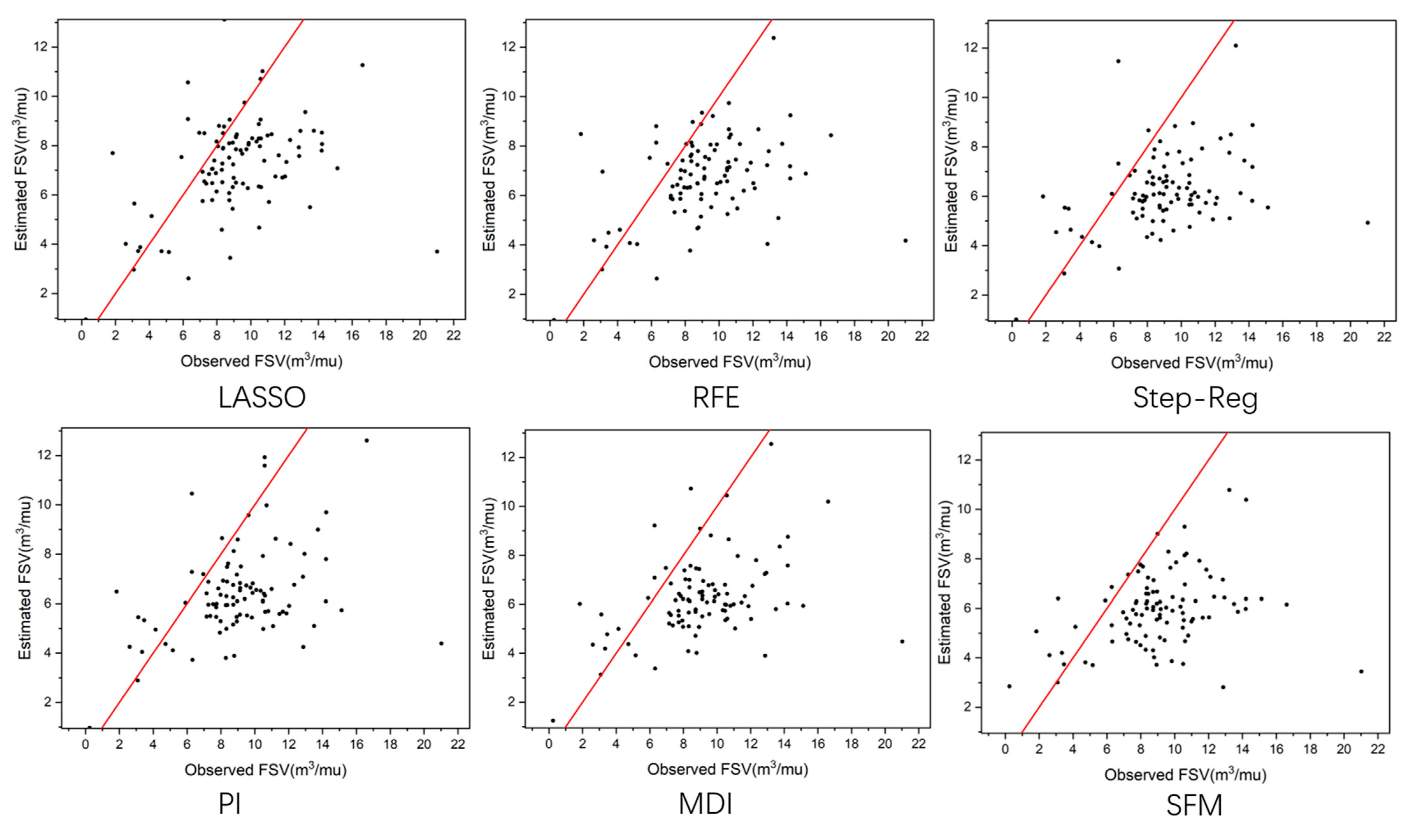
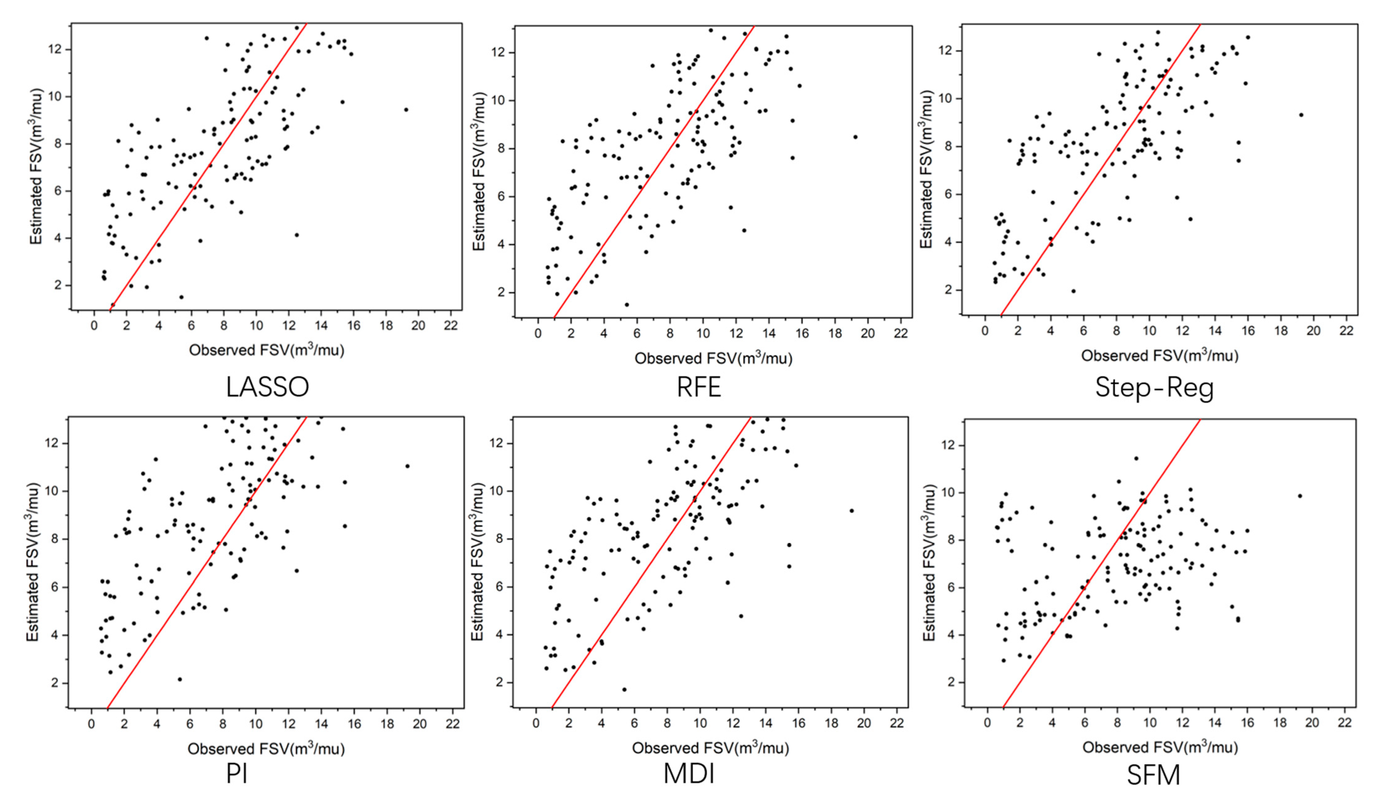
Additionally, Table A1 exhibited that R² of broad-leaved in Longquan area was negative. Figure A1 delineates the scatter plot graph of the estimated and observed FSV of the broad-leaved in Longquan City. In Figure A1, we noticed the phenomenon showed that the fitted result of broad-leaved in this area is poor. Table 1 showed that the sample amount of broad-leaved in Longquan City is only 101, and the total amount of broad-leaved is 16,913, accounting for less than 0.6%. However, the sample amount of Masson pine in Longquan City is only 154, and the total amount of Masson pine is 9425, accounting for only 1.6%. Figure A2 shows the scatter plot graph of the estimated and observed FSV of the Masson pine in Longquan City. Both of their performances were worse than the same dominant tree species in the other two regions. At the same time, from Table A1 and Figure A1, it was found that whether all the feature variables were selected or part of the feature variables selected after feature selection, the FSV of broad-leaved in Longquan result was poor. Therefore, it was speculated that the poor estimated results might be due to the uneven distribution of broad-leaved in Longquan area, or the sample data of broad-leaved in Longquan area having too much noisy data. In a word, the small scale and minimal diversity of dominant tree species may lead to unstable and unreliable experimental results, which is the same idea held by Zhou et al. [24].

In order to observe the robustness and explanation of the selected features to different tree species and verify the regional universality of different feature selection methods we averaged the results of the test area of the same tree species, and obtained the results as shown in

Table 7. FSV estimation accuracy assessments on validation dataset on average among three areas.

Dominant Tree Species	Variable Selection Method	R2	RMSE(m3/mu)
	LASSO	0.3178	1.7599
	RFE	0.1477	1.9380
Broad-leaved	Step-Reg PI MDI SFM None	0.1512 0.2387 0.1679 0.2137 0.1986	1.1881 1.8469 1.9222 1.9118 1.8961
Coniferous	LASSO RFE Step-Reg PI MDI SFM None	0.5969 0.6252 0.6024 0.6169 0.6125 0.6106 0.5990	1.8031 1.7514 1.7932 1.7677 1.7738 1.7873 1.7967
Chinese Fir	LASSO RFE Step-Reg PI MDI SFM None	0.7303 0.7379 0.7248 0.7434 0.7389 0.7204 0.7367	1.7796 1.7534 1.7986 1.7376 1.7537 1.8194 1.7560
Masson Pine	LASSO RFE Step-Reg PI MDI SFM None	0.6868 0.7017 0.7025 0.6871 0.7034 0.4501 0.7021	1.9006 1.8514 1.8527 1.9027 1.8543 2.4861 1.8596
Mixed	LASSO RFE Step-Reg PI MDI SFM None	0.5720 0.5917 0.5879 0.5890 0.5953 0.4528 0.5874	1.7426 1.7081 1.7133 1.7119 1.9590 1.9590 1.7153
All	LASSO RFE Step-Reg PI MDI SFM None	0.7835 0.7972 0.7949 0.7983 0.7968 0.7928 0.7925	1.6758 1.6207 1.6291 1.6154 1.6427 1.6388 1.6238

.

According to the results of Table 6, Table 7, Table A1 and Table A2, except for broad-leaved owing to the bad-fitting in Longquan, we compared the top three best performance of the results. Through compared variable selection methods of the average results with those of the results of tree species of the separate three regions comprehensively, what we could find was as follows. In the feature selection of coniferous, RFE performed better both in the average and in the separate regions. In the feature selection of Chinese fir and all, PI performed better both in the average and in the separate regions. In the feature selection of Masson pine, MDI performed better both in the average and in the separate regions. However, in the feature selection of mixed, MDI performed better in the average while RFE performed better in the separate regions comprehensively. From the results of the mixed species, we found that in Longquan and Anji the results between MDI and RFE were considerably close, while in Lin’an the results in MDI were a lot better than RFE, which is the reason why MDI is the best result in the average result.

6. Discussion

The purpose of this study was to use satellite imagery data, terrain data, and forest inventory data as feature variables to estimate the FSV of six dominant tree species in different regions by using different variable selection methods, and to explore the better performance of variable selection methods according to the predicted results. FSV is an important variable in forest management reports at the provincial and national levels. Using Sentinel-2A imageries to process and establish models to estimate FSV maps is particularly important in southern China. One of the reasons for this is that forestry inventory in southern China is an important part of China’s forestry [43]. In addition, feature selection methods can lead to the reduction of high-dimensional data, minimize the data storage space, and improve the interpretability of the model. Consequently, it was used to improve the performance of the prediction model. In order to explore which variable selection approach has better performance on the same type of dominant tree species in different regions, six feature selection algorithms, LASSO, RFE, Step-Reg, PI, MDI, and SFM, were selected and combined with XGBoost.

Based on forest inventory data, Sentinel-2A spectral bands, terrain factors, vegetation indices, and texture features extracted by Sentinel-2A imageries, this study explored the performance about the FSV in different regions through using six feature selection algorithms combined with XGBoost. The results exhibited that the variable selection methods can select the best-performing features, which would change according to different dominant tree types or the same dominant tree type in different regions. From Table 6, Table A1 and Table A2, we found that the variables selected by SFM performed unstably. Moreover, from the average results of the three regions, we found that the feature selection algorithm was better than those that had no use of feature selection. It showed that using partial feature selection can reduce capacity of data storage space, make models more explanatory, and make the predicted results more accurate. In other words, variable selection is conducive to improving the performance of FSV estimation, and this conclusion is consistent with the conclusion Li et al. obtained [43].

From the FSV estimated results of three regions, all tree species estimation performed better than the classified tree estimated error. This result was consistent with [44] forest growth simulation, which used kNN to estimate the FSV based on Landsat TM imagery and forest field survey data at the stand level. The results of this study showed that the FSV estimation errors of different tree species are significantly higher than the overall estimation errors. At the same time, when exploring the more important features of each dominant tree type’s dataset, the importance of tree age and canopy density is very important for the prediction of FSV of multiple dominant tree types, and the multiple features in forest inventory data are important for the accurate prediction of FSV.

In the study, the amount of broad-leaved in Longquan is small, and the final estimated results were poor, while the predicted results of broad-leaved in other two areas are better. Besides, from Table 1, we found that in broad-leaved, the dominant tree in three regions could be drawn that Longquan< Anji< Lin’an. In Masson pine, it could be drawn that Longquan< Anji <Lin’an. In coniferous, it could be drawn that Anji < Longquan < Lin’an. In the best performance of these dominant tree species, we found that in broad-leaved, it could be drawn that Longquan < Anji < Lin’an. In Masson pine, however, it could be drawn that Longquan < Lin’an < Anji. In coniferous, it could be drawn that Anji < Lin’an < Longquan. Although broad-leaved and Masson pine in Longquan only account for 0.60% and 1.63% of all the broad-leaved and Masson pine in three regions, respectively, Masson pine’s fitting results have reached the qualified correlation index (R² > 0.6), while R² in broad-leaved were all negative. From Figure A1 and Figure A2, it is obvious that the fitting results of Masson pine are much better than broad-leaved, which showed that the small amount is not the only reason for bad fitting. On the contrary, we noticed that Masson pine in Anji and Lin’an, respectively, account for 19.18% and 79.18% in all Masson pine, while Chinese fir in Lin’an and Longquan account for 64.82% and 22.61%, respectively. From both of the results, we found that if the samples occupy enough in the whole dominant tree species, the results were not affected by the amount of the samples. We draw a conclusion that the small-scale and diversity of tree species may lead to the instability and unreliability of experimental results, which is the same as Zhou et al. [24] considered.

From Table 6, Table A1 and Table A2, we found that whether it was classified by tree species or by regions, MDI, PI and RFE performed well. From Table 7, the top three performance of the variable selections of the average results showed that MDI, PI, and RFE also have good performance. Whether in the average or in the separate regions, their final estimated results were terribly close. Luo et al. [18] used three variable selection methods and three machine learning algorithms to estimate the AGB and found that the combination of RFE for variable selection and CatBoost as the regression approach got the best accuracy, which showed that RFE is an effective method to optimize the variables. In the meanwhile, not only RFE, but MDI and PI, were recommended for variable selection to estimate the FSV.

With further research, the estimated effect may be further improved. This study is still applied to some forest inventory data, most of which still needs to be collected artificially in the field. Future studies may consider using radar or satellite imagery to study forest accumulation estimation through in-depth learning and fusion of satellite imagery in isolation from these artificial factors.

7. Conclusions

In this study, six dominant tree species were selected in Lin’an District, Anji County, and Longquan City. The FSV of tree species in each area was estimated by using different variable selection methods combined with XGBoost. The regional suitability of different feature selection methods in each tree species was studied through average results, and three conclusions were drawn from data analysis. The following conclusion can be drawn:

(1)

MDI, PI, and RFE were recommended to select variables in dominant tree species from different regions.

(2)

Feature selection methods that simultaneously select the optimal features will change according to different tree types, and they are crucial to improve the accuracy of forest stock volume estimation. Moreover, tree age and canopy density were of great importance to the estimation of the FSV.

(3)

The small size and diversity of dominant tree types might cause the experiment results to be unstable and unreliable. Furthermore, if the number of tree samples is big enough, the above bad-fitting condition would not easily depend on the number.

References

- Mohammadi, J.; Shataee Joibary, S.; Yaghmaee, F.; Mahiny, A.S. Modelling forest stand volume and tree density using Landsat ETM+ data. Int. J. Remote Sens. 2010, 31, 2959–2975. [Google Scholar] [CrossRef]
- FAO (Food and Agriculture Organization of the United Nations). Global Forest Resources Assessment Update 2005: Terms and Definitions. 2004. Available online: https://www.fao.org/3/ae156e/AE156E00.htm (accessed on 20 October 2021).
- Næsset, E.; Gobakken, T.; Bollandsås, O.M.; Gregoire, T.G.; Nelson, R.; Ståhl, G. Comparison of precision of biomass estimates in regional field sample surveys and airborne LiDAR-assisted surveys in Hedmark County, Norway. Remote Sens. Environ. 2013, 130, 108–120. [Google Scholar] [CrossRef] [Green Version]
- Santoro, M.; Cartus, O.; Fransson, J.E.; Shvidenko, A.; McCallum, I.; Hall, R.J.; Beaudoin, A.; Beer, C.; Schmullius, C. Estimates of forest growing stock volume for sweden, central siberia, and québec using envisat advanced synthetic aperture radar backscatter data. Remote Sens. 2013, 5, 4503–4532. [Google Scholar] [CrossRef] [Green Version]
- Lindberg, E.; Hollaus, M. Comparison of methods for estimation of stem volume, stem number and basal area from airborne laser scanning data in a hemi-boreal forest. Remote Sens. 2012, 4, 1004–1023. [Google Scholar] [CrossRef] [Green Version]
- Tomppo, E.; Nilsson, M.; Rosengren, M.; Aalto, P.; Kennedy, P. Simultaneous use of Landsat-TM and IRS-1C WiFS data in estimating large area tree stem volume and aboveground biomass. Remote Sens. Environ. 2002, 82, 156–171. [Google Scholar] [CrossRef]
- Merino-de-Miguel, S.; González-Alonso, F.; García-Gigorro, S.; Roldán-Zamarrón, A.; Cuevas, J.M. Forest biomass estimation through NDVI composites. The role of remotely sensed data to assess Spanish forests as carbon sinks. Int. J. Remote Sens. 2006, 27, 5409–5415. [Google Scholar]
- Ahmed, R.; Siqueira, P.; Hensley, S. A study of forest biomass estimates from LiDAR in the northern temperate forests of New England. Remote Sens. Environ. 2013, 130, 121–135. [Google Scholar] [CrossRef]
- Chao, Z.; Dao-li, P.; Yun-yan, T.; Yong-feng, D.; Chang-gui, Z. Predicting forest volume in Three Gorges Reservoir Region using TM images and partial least squares regression. J. Beijing For. Univ. 2013, 35, 11–17. [Google Scholar]
- Mura, M.; Bottalico, F.; Giannetti, F.; Bertani, R.; Giannini, R.; Mancini, M.; Orlandini, S.; Travaglini, D.; Chirici, G. Exploiting the capabilities of the Sentinel-2 multi spectral instrument for predicting growing stock volume in forest ecosystems. Int. J. Appl. Earth Obs. Geoinf. 2018, 66, 126–134. [Google Scholar] [CrossRef]
- Pang, X.; Liu, H.; Nian, X. Estimating Forest Volume Using Sentinel—2A Satellite Remote Sensing Image. J. Northeast For. Univ. 2021, 49, 72–77. [Google Scholar] [CrossRef]
- Li, L.; Zhou, X.; Chen, L.; Chen, L.; Zhang, Y.; Liu, Y. Estimating urban vegetation biomass from Sentinel-2A image data. Forests 2020, 11, 125. [Google Scholar] [CrossRef] [Green Version]
- Li, D.; Gu, X.; Pang, Y.; Chen, B.; Liu, L. Estimation of forest aboveground biomass and leaf area index based on digital aerial photograph data in Northeast China. Forests 2018, 9, 275. [Google Scholar] [CrossRef] [Green Version]
- Li, K.; Wu, D.; Fang, L. Forest Volume Stock with Sentinel—2 Remote Sensing Image. J. Northeast For. Univ. 2021, 49, 59–66. [Google Scholar]
- Obata, S.; Cieszewski, C.J.; Lowe, R.C.; Bettinger, P. Random Forest Regression Model for Estimation of the Growing Stock Volumes in Georgia, USA, Using Dense Landsat Time Series and FIA Dataset. Remote Sens. 2021, 13, 218. [Google Scholar] [CrossRef]
- Huang, Y.L.; Wu, D.S.; Fang, L.M. Forest stock volume estimation based on XGboost method of stepwise regression. J. Cent. South Univ. For. Technol. 2020, 40, 72–80. [Google Scholar]
- Li, S.B.; Lin, H.; Wang, G.M.; Cheng, T.L. Estimation of forest volume based on GF-1. J. Cent. South Univ. For. Technol. 2019, 39, 70–75. [Google Scholar]
- Luo, M.; Wang, Y.; Xie, Y.; Zhou, L.; Qiao, J.; Qiu, S.; Sun, Y. Combination of feature selection and catboost for prediction: The first application to the estimation of aboveground biomass. Forests 2021, 12, 216. [Google Scholar] [CrossRef]
- Yu, X.; Ge, H.; Lu, D.; Zhang, M.; Lai, Z.; Yao, R. Comparative study on variable selection approaches in establishment of remote sensing model for forest biomass estimation. Remote Sens. 2019, 11, 1437. [Google Scholar] [CrossRef] [Green Version]
- Lu, D.; Chen, Q.; Wang, G. A survey of remote sensing-based aboveground biomass estimation methods in forest ecosystems. Int. J. Digit. Earth 2016, 9, 63–105. [Google Scholar] [CrossRef]
- Lieth, H. Patterns of Primary Production in the Biosphere; Dowden, Hutchinson & Ross: Strouds-burg, PA, USA, 1978. [Google Scholar]
- Georganos, S.; Grippa, T.; Vanhuysse, S.; Lennert, M.; Shimoni, M.; Kalogirou, S.; Wolff, E. Less is more: Optimizing classification performance through feature selection in a very-high-resolution remote sensing object-based urban application. GIScience Remote Sens. 2018, 55, 221–242. [Google Scholar] [CrossRef]
- Li, X.; Lin, H.; Long, J. Mapping the growing stem volume of the coniferous plantations in North China using multispectral data from integrated GF-2 and Sentinel-2 images and an optimized Feature variable selection method. Remote Sens. 2021, 13, 2740. [Google Scholar] [CrossRef]
- Zhou, R.; Wu, D.; Fang, L.; Xu, A.; Lou, X. A Levenberg–Marquardt backpropagation neural network for predicting forest growing stock based on the least-squares equation fitting parameters. Forests 2018, 9, 757. [Google Scholar] [CrossRef] [Green Version]
- McRoberts, R.E.; Gobakken, T.; Næsset, E. Post-stratified estimation of forest area and growing stock volume using lidar-based stratifications. Remote Sens. Environ. 2012, 125, 157–166. [Google Scholar] [CrossRef]
- Zhao, G.Q.; Zhao, H.; Feng, S.C. Carbon storage characteristics of forest vegetation in Anji county of Zhejiang province. J. Northwest For. Univ. 2017, 32, 82–85. [Google Scholar]
- He, Y.; Huang, C.; Li, H.; Liu, Q.S.; Liu, G.H.; Zhou, Z.C.; Zhang, C.C. Land-cover classification of random forest based on Sentinel- 2A image feature optimization. Resour. Sci. 2019, 41, 992–1001. [Google Scholar] [CrossRef]
- Astola, H.; Häme, T.; Sirro, L. Comparison of Sentinel-2 and Landsat 8 imagery for forest variable prediction in boreal region. Remote Sens. Environ. 2019, 223, 257–273. [Google Scholar] [CrossRef]
- Gao, L.L. Inversion of the Apple Tree Canopy Chlorophyll Contents in Hilly Region Based on Remote Sensing Data. MA Thesis, Shandong Agricultural University, Taian, China, 2017. [Google Scholar]
- Zhang, W.C.; Liu, H.B.; Wu, W. Classification of land use in low mountain and hilly area based on random forest and Sentinel-2 satellite data: A case study of Lishi Town, Jiangjin, Chongqing. Resour. Environ. Yangtze Basin 2019, 28, 1334–1343. [Google Scholar]
- Hu, Y.; Xu, X.; Wu, F. Estimating forest stock volume in Hunan Province, China, by integrating in situ plot data, Sentinel-2 images, and linear and machine learning regression models. Remote Sens. 2020, 12, 186. [Google Scholar] [CrossRef] [Green Version]
- Haralick, R.M.; Shanmugam, K.; Dinstein, I.H. Textural features for image classification. IEEE Trans. Syst. Man Cybern. 1973, 6, 610–621. [Google Scholar] [CrossRef] [Green Version]
- Singh, D.; Singh, B. Investigating the impact of data normalization on classification performance. Appl. Soft Comput. 2020, 97, 105524. [Google Scholar] [CrossRef]
- Shao, J. Linear model selection by cross-validation. J. Am. Stat. Assoc. 1993, 88, 486–494. [Google Scholar] [CrossRef]
- Liu, B. Automatic Coloring Method for National Costume Sketches. MA Thesis, Yunnan Normal University, Kunming, China, 2020. [Google Scholar] [CrossRef]
- Li, L.; Wu, Y.; Ye, M. Survey on feature engineering of image holistic scene understanding based on probabilistic graphical model. Appl. Res. Comput. 2015, 32, 3542–3550. [Google Scholar]
- Zhiqin, L.; Jianqiang, D.; Bin, N. Summary of feature selection methods. Comput. Eng. Appl. 2019, 55, 10–19. [Google Scholar]
- Guyon, I.; Weston, J.; Barnhill, S. Gene selection for cancer classification using support vector machines. Mach. Learn. 2002, 46, 389–422. [Google Scholar] [CrossRef]
- Lomax, R.G. Statistical concepts: A Second Course for Education and the Behavioral Sciences; Lawrence Erlbaum Associates Publishers: Mahwah, NJ, USA, 2001. [Google Scholar]
- Breiman, L. Random forests. Mach. Learn. 2001, 45, 5–32. [Google Scholar] [CrossRef] [Green Version]
- Chen, T.; Guestrin, C. Xgboost: A scalable tree boosting system. In Proceedings of the 22nd ACM SIGKDD International Conference on Knowledge Discovery and Data Mining, San Francisco, CA, USA, 13–17 August 2016; pp. 785–794. [Google Scholar]
- Zhanshan, L.; Zhaogeng, L. Feature selection algorithm based on XGBoost. J. Commun. 2019, 40, 101. [Google Scholar]
- Li, Y.; Li, C.; Li, M. Influence of variable selection and forest type on forest aboveground biomass estimation using machine learning algorithms. Forests 2019, 10, 1073. [Google Scholar] [CrossRef] [Green Version]
- Mäkelä, H.; Pekkarinen, A. Estimation of forest stand volumes by Landsat TM imagery and stand-level field-inventory data. For. Ecol. Manag. 2004, 196, 245–255. [Google Scholar] [CrossRef]
Figure 1.
Zhejiang province in East China and the study area, shown in a natural color composite image from Sentinel-2A.