
A Tool for Long-Term Forest Stand Projections of Swedish Forests

Department of Forestry and Wood Technology, Linnaeus University, 351 06 Växjö, Sweden
*
Author to whom correspondence should be addressed.
Forests 2022, 13(6), 816; https://0-doi-org.brum.beds.ac.uk/10.3390/f13060816
Submission received: 29 March 2022
/
Revised: 17 May 2022
/
Accepted: 20 May 2022
/
Published: 24 May 2022
(This article belongs to the Section Forest Ecology and Management)
Abstract
:The analysis of forest management strategies at landscape and regional levels forms a vital part of finding viable directions that will satisfy the many services expected of forests. This article describes the structure and content of a stand simulator, GAYA, which has been adapted to Swedish conditions. The main advantage of the GAYA implementation compared to other resources is that it generates a large number of management programmes within a limited time frame. This is valuable in cases where the management programmes appear as activities in linear programming (LP) problems. Two methods that are engaged in the projections, a climate change response function and a soil carbon model, are designed to complement other methods, offering transparency and computational effectiveness. GAYA is benchmarked against projections from the Heureka system for a large set of National Forest Inventory (NFI) plots. The long-term increment for the entire NFI set is smaller for GAYA compared with Heureka, which can be attributed to different approaches for modelling the establishment of new forests. The carbon pool belonging to living trees shows the same trend when correlated to standing volume. The soil carbon pool of GAYA increases with increased standing volume, while Heureka maintains the same amount over the 100-year projection period.
1. Introduction
Forests are expected to fulfil a range of services that elicit competing interests. The Intergovernmental Panel on Climate Change (IPCC) point to the critical role of forests in climate mitigation [1], the EU ‘Fit for 55’ package of proposals [2] puts a strong emphasis on biodiversity, while the work on National Forestry Programmes [3] brings in other aspects that relate to the role of forests in the national economy. The need for effective analysis tools in the domain of forestry for revealing trade-offs and for help in negotiating effective strategies has probably never been more important.
Long-term analyses of forest management that goes beyond the stand level need models that can project the plausible development of the multitude of elements that make up the forest, whether it is a small forest holding, a landscape, the forest of a whole country, or an even larger region. The forest element could be a stand, a sample plot, a pixel or whatever is managed as one object for silvicultural interventions (henceforth, reference will be made to the term ‘stand’ in a general context). The dominating approach for large-scale and long-term forest management analysis is to have a separate growth and yield simulator that feeds data into the problem solver where the management problem is expressed [4]. That gives freedom as to what data, techniques, and models are used in the simulator. There are exceptions—for instance, where Markov models are embedded in the forest-level management problem [5,6,7,8].
There are many growth and yield models; however, not all of them qualify as stand simulators for the purposes mentioned above. In particular, a stand simulator needs the flexibility to represent different forests, not only a particular piece of land, and to simulate the range of forest management methods that are relevant for the solution of different management problems. In short, a stand simulator that serves as part of a system for analysis should have the capacity to cover a reasonable problem domain. Among the more established systems that encompass stand simulators are AFFOREST-sDSS, DSD, EFIMOD, EMDS, ETÇAP, FORESTAR, Heureka, Kupolis, LANDIS, MELA, Monsu, Monte, ProgettoBosco, SADfLOR, Sibyla, SILVA, and Woodstock [9]. Almost all are based on empirical growth relationships, although process-based or hybrid models, such as FORMIT-M [10], SILVA [11], and 3PG [12], are currently gaining some interest. One reason for this is the possibility of their better simulating responses to climate change compared to empirical models.
A distinction can be made between stand simulators that serve forest management problems that could be called ‘strategy evaluation’ and those that could be called ‘strategy development’. The former would have a management strategy prescribed, and the task is to evaluate the performance against a set of criteria. This means working sequentially through the planning periods, applying the strategy at each stage, as with EFIMOD [13], Heureka/RegWise [14], Kupolis [15], Sibyla [16], and SILVA [17]. Strategy development would instead entail providing a range of options for each stand and combining them in an optimal way against the criteria to find the management strategy. In contrast to the strategy evaluation problem, the strategy development problem requires that the stand simulator has the capacity to generate an adequate number of management programmes to represent all of the relevant options that could theoretically form an optimal strategy.
Among the more established systems for strategy development, problem formulation often takes the form of a linear programming (LP) problem, with a structure first defined by Johnson and Scheurman [18]. A management programme, in this context, is a given sequence of forest management actions at stand level. The management programmes from the stand simulator form (part of) the columns of the LP model. MELA [19], Monsu [20], SADfLOR [21], and Heureka/PlanWise [14] are examples of systems that follow this approach for forest-level problems; FASOM [22], NorFor [23], and SweFor [24] are among inter-temporal optimization forest sector models with the same structure. The difference between forest-level systems and sector models is more one of scale than of kind; the role of the stand simulator is the same, i.e., to provide an adequate number of management programmes.
Swedish forestry has experienced at least two generations of forest decision support systems, the first represented by FMPP [25] and Hugin [26], and the second by Heureka/PlanWise and Heureka/RegWise [14]. FMPP and Heureka/PlanWise are more directed at dealing with forest-level problems, whereas Hugin and Heureka/RegWise are designed for national and regional analyses based on National Forest Inventory (NFI) sample plots [27]. Heureka/PlanWise and Heureka/RegWise share the same set of growth and yield functions. Heureka is the de facto industry standard for long-term forest management analyses in Sweden. It is used by all major forest companies and many medium-sized forest owners and is the source of an extensive number of scientific publications [28]. However, as a tool for management program generation, Heureka/PlanWise has limitations. Those that can be more serious in an experimental or research setting are that, firstly, of all the permissible management programs, only a few are generated (and for some applications too few); secondly, the criterion for selecting management programs is net present value (which may not be your main target); and finally, many controls lack documentation, which means you tend to be content with default settings whether that is in line with your study objectives or not.
GAYA is a dedicated tool for computing management programs for inclusion in LP problems. It was originally developed at SLU [29] and given a more thorough description at the Norwegian institute for forest research (NISK) [30]. Various scientific publications relate to its applications, e.g., in Sweden [31], Norway [32], Iran [33], Latvia, and Ukraine (one of the authors of the current paper acted as consultant on the two latter examples). The various applications are made possible while GAYA is a shell under which the user can input growth end yield functions and other relationships for producing management programmes. The aim of this article is, firstly, to present the structure of the projection system. Its simplicity and computational efficiency could be of general interest. Secondly, a comprehensive description of an up-to-date implementation of GAYA for Swedish conditions is presented. This includes a simple model for climate change impact on growth related to IPCC scenarios and an abbreviated method for carbon accounting; both should contribute to the capacity to generate many management programmes while still being in control of the user.
The next two sections describe the content of the GAYA implementation, including the climate change model and the carbon accounting method. Then, there is a benchmark of the GAYA implementation against the Heureka system. The article concludes with a discussion of the benchmark study and an analysis of what niche among forest simulators GAYA implementation could fill.
2. Materials and Methods
GAYA is designed to yield a large set of management programs to feed into an analysis tool, normally an LP solver. A management programme either runs from the start of the planning period to its end, consistent with the definition of programmes for a Model I, or until final harvest, consistent with a Model II [18]. To understand how projections are made, first, there is an outline of the overall structure and flow control. Then, we give a detailed description of how growth projections are made, a simplified method for climate change growth effects, and a procedure for computing the size of forest carbon pools.
2.1. Structure and Control
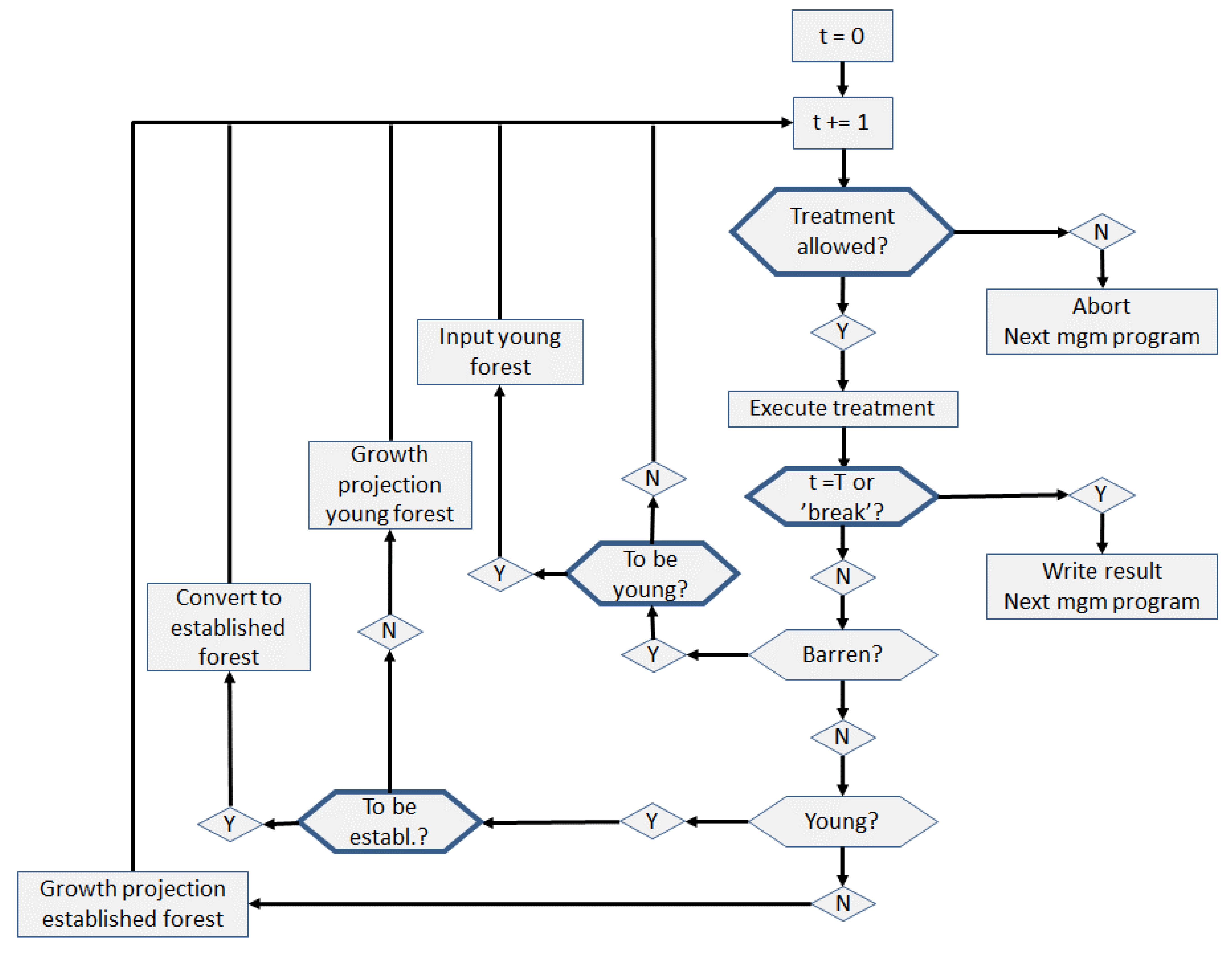
Figure 1 describes the procedure for making one management program for a stand with a planning horizon of T periods divided into 5-year periods. The projection ends if either the end of the planning horizon has been reached, a ‘break’ treatment is simulated, or if the suggested treatment is not allowed and the computation is aborted. The projection for period t starts by simulating the treatment followed by an update of the state after treatment. The growth of the stand is then projected and the projection for period t + 1 begins. As of now, GAYA is only able to handle area production models, i.e., it relies on stand averages and does not include diameter distributions or other such structural data.
A stand can be in one of three states: barren, young, or established. The update of the state of the forest depends on whether the ground is barren (there are no trees), if it is young forest (the stand does contain trees but no basal area), or if it is established (there are trees with basal area). The workflow for projecting the stand one period is as follows:
- The stand is in a defined state in period t. Whether a particular kind of treatment is allowed or not is defined by the user in terms of stand conditions. Thus, the treatment rules for the kind of treatment that is prescribed for period t is checked against the state of the stand. If allowed, the next step is to execute the treatment and update stand conditions after treatment; otherwise, the programme is aborted.
- After simulation of the treatment and update, the next check is to determine if the end of the planning period is reached (t = T) or if the treatment is defined as a ‘break’ treatment, e.g., final felling. If management programmes are aimed at an LP application, the ending condition depends on whether it is a Model I or Model II application, respectively.
- In the case of barren land, the projection is simply an update of time since it became barren. If certain user-defined conditions are met, a given composition of young forest is imported, and the state of the stand is transferred to young forest. Thus, regeneration is not an available treatment in GAYA; the regeneration phase of the stand development process is implicit in the imported young stand.
- The young stand has a number of trees that develop in, for instance, number and height, depending on what growth functions are implemented. Once certain user-defined conditions are met, the stand is converted to established forest, i.e., it is assigned a basal area. Other stand variables may also be updated.
- The established forest stand is projected with respect to all stand variables that are relevant in the particular case.
GAYA as a shell for stand management program generation leaves much of the control to the user. The following is supplied by the user:
- Definitions of treatments and rules for when they are allowed, and assignment of the ‘break’ treatment, if any.
- The young forest states that should be imported, and the rules for when a particular young forest should be used to convert barren land to young forest.
- The rules for when a young forest should be converted to established forest.
- Growth and yield functions in sub-routines for barren, young, and established forest, respectively.
- One sub-routine for simulating treatments (removal of trees, cost and assortments calculation).
- Two sub-routines for communicating with external data: one for reading the stand register and young forest definitions, and one for writing the result of a management programme.
The rules for controlling treatments, and when to convert barren land to young forest and young forest to established forest, are given with a Boolean expression based on stand conditions. They reside in an ordinary text file together with other specifications to control the workflow.
The following forms of silvicultural treatments are available:
Undisturbed growth: The stand is left as is.
Pre-commercial thinning: A number of stems are removed; either the number of stems to be removed or the number of stems after pre-commercial thinning are specified. The removal can be geared towards specific species. The treatment is only eligible for young forest.
Thinning: A number of stems are removed with a relative diameter. The treatment can be specified in different ways, for instance by combining thinning strength on basal area with number of stems to remove, or by basal area after thinning and number of stems after thinning. The treatment is only eligible for established forest.
Fertilization: Fertilization is specified in terms of type of fertilizer and amount. The treatment is only eligible for established forest.
Thinning in combination with fertilization: The combined treatment is specified for thinning and fertilization, respectively, as described above.
Final felling: All trees are removed and the stand is turned into barren land. The treatment is only eligible for established forest.
There are different methods available for generating the sequence of treatments that constitute the management programme. The only method that has been used so far in research projects is complete enumeration, i.e., all conceivable combinations of treatments that are eligible are reported. The totality of potential management programmes is for most applications considerable. Thus, the specification of treatment rules becomes crucial in order to limit the number of programmes and only maintain those that potentially could enter the solution. The generation of management programmes is computationally enhanced by working backwards in a tree-like structure, with the root in period one and branching off in each period.
2.2. Swedish Growth Projection Implementation
2.2.1. Barren Land
This phase covers the instance where the stand has no stems at all or few stems of low height, i.e., less than 100 ha−1 and with average height less than 1.3 m. It is either the initial state or occurs after a simulated final felling. It is assumed that the stand is regenerated and that 5 years are added for each period. Once the stand reaches a dominant height of 1.3 m according to Hägglund [34,35,36], the stand is assigned stems and age for different species for the young forest corresponding to region and vegetation type of the stand. Currently, there is a register of 48 young forest descriptions differentiated on three regions (north, middle, and south Sweden) and 16 different forest vegetation types within each region. They originate from an analysis of 1923 NFI plots from the years 2016–2018 in the height range of 1.3 to 3 metres.
2.2.2. Young Forest
Young forest is represented by stands with stems and the age of different species but with no basal area. Age is updated with five years and the number of stems adjusted by pre-commercial thinning if applied. Each species is assigned a volume according to [37]. Once the height of the dominant species reaches 8.5 m, according to Hägglund [34,35,36], all species are assigned basal areas with form factors from Table 1 and thus transferred to the established forest.
2.2.3. Established Forest
The growth of established forest is the most critical part of a projection in the sense that it is during this phase that most of the ecosystem services are provided. This is also where there is a greater number of different models to consider in order to arrive at a new state of the stand after treatment. The Swedish tradition in production research, established at least half a century ago, is to assess the basal area growth, and possibly also height increment, followed by a static calculation of volume. This is also how the earlier systems, Hugin and FMPP, and also the Heureka system, organize growth projection. The following steps are followed to make a five-year projection:
- Basal area growth is predicted with Elfving’s single tree model [38,39], except for lodgepole pine, which uses the area production model of the Hugin system [26]. The tree population is represented by the stand mean tree. Since Elfving’s model [38] is a single tree model, this could lead to an overestimation of growth. This will be further investigated in Section 3.2.
- The basal area growth is multiplied with a breeding factor and a climate effect factor. The breeding factor applies for stands for which the initial state is barren land or are finally felled during the projection period. The current practical breeding effect is set to 10%, which increases by 0.375% per year (the theoretical effect of 0.5% is reduced by 75% due to pollen external to the orchard) [40]. The climate effect function is presented in Section 2.3.
- Natural mortality is computed for each species as a removal of a relative share of basal area. The calculations depend on whether the basal area is above or below a limit defined by Söderberg [41]. Functions according to Söderberg [41] are used for basal areas larger than a limit, and functions according to Bengtsson [42] for basal areas smaller than the limit. The same proportion of the number of trees is removed, i.e., the relative diameter of natural mortality is assumed to be one.
- The basal area and number of trees passing over the 5 cm limit, i.e., ingrowth, are computed following Wikberg [43].
- If fertilization takes place, the basal area growth is multiplied with a fertilization effect according to Pettersson [44], with one value for the current period and another value for the following period. The effect is reduced by 50% for species other than Scots pine and Norway spruce.
- The new state—after adjustment for growth (including breeding and climate effects), natural mortality, ingrowth, and fertilization—is used to compute the volume of each species. Functions by Agestam [45] are applied, except for oak and beech, where functions by Hagberg and Matérn [46] are applied. An alternative to [45] is the single tree models by Brandel [47]. Both [45,47] were tried with a set of established NFI plots from year 2018. Ref [45] comes close to the current growth rate of 5.2 m3ob ha−1 y−1 reported by Nilsson et al. [27], whereas [47] approaches 6.6 m3ob ha−1 y−1. A reason for the overstatement of [47] could be that it is a single tree model, while [45] is based on stand average data.
2.3. Climate Change Growth Effects
The transient dynamic regional climate scenarios used in this study were obtained from the regional RCA3 climate model—using global driving variables from the general circulation model ECHAM4/OPYC3—by the Swedish Meteorological and Hydrological Institute [48]. Two scenarios were used in the simulations, based on two emission scenarios, B2 and A2, in which [CO2] = 572 and 726 ppm in the year 2085, respectively [49]. The global mean warming during this century is 3.6 °C for the A2 scenario and 2.5 °C for the B2 scenario. The relative increase in precipitation is higher in northern Sweden, while in south-eastern Sweden there is a slight decrease in annual humidity. There is a relative decrease in precipitation for both scenarios during the summer months (June–August), especially for the A2 scenario, where the decrease is >20% at the end of this century compared with present climate.
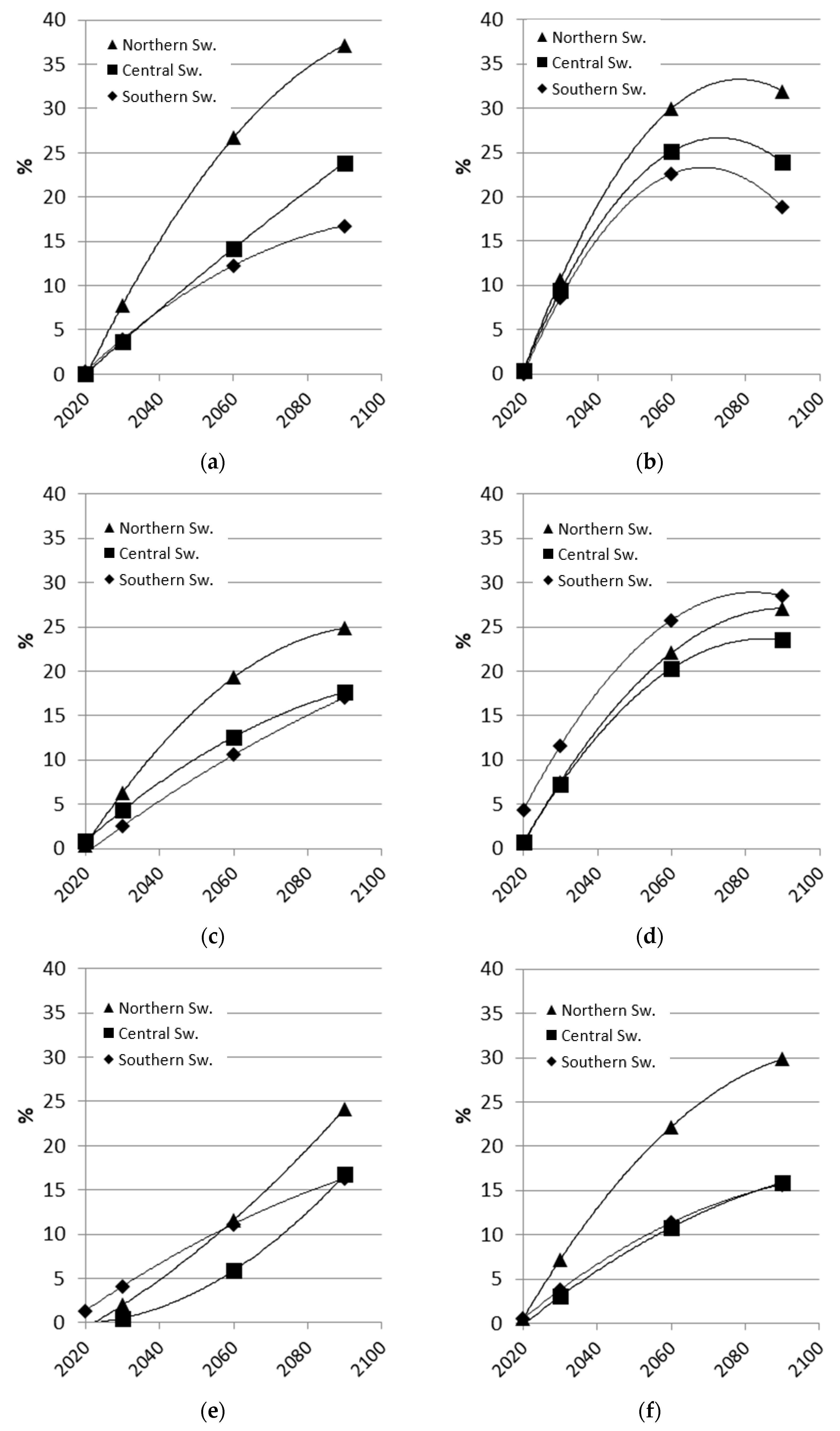
The model simulations are performed with the process-based model BIOMASS for the period 2015–2100 with climate data calculated using B2 and A2 scenarios as a basis [50]. Production changes have been estimated for spruce, pine, and deciduous species. Output data from the model include net primary production (NPP), which can be seen as a measure of how growth can change. It is in good agreement with previous estimates [50]. This estimate does not include the potential positive effect of increased nutrient turnover in the soil, nor any possible loss of production as a result of increased damages. To differentiate production development over Sweden, data is divided between southern (<59′ N), central (59−63′ N), and northern (>63′ N) Sweden. The output from BIOMASS is generalized with regression for the period 2015–2100 (Table 2; Figure 2) with function
where R is the relative change of production and y is the year between 2020–2100 (2020, 2025…).
2.4. Biomass Stocks and Decay
The climate mitigation net effect of forest strategies depends both on changes of stocks in the forest as well as substitution effects and stock changes related to harvested wood products. Many studies indicate that the former tends to have a larger impact than the latter. Thus, the forest stocks of different fractions and their decay are of prime importance for arriving at a qualified assessment of the climate regulatory service of a forest strategy.
The carbon accounting model presented here is not an integral part of GAYA as such. However, the classifications and the data needs of the carbon model have direct implications for the data that is delivered from the management programmes. The intention of carbon accounting in connection with the use of GAYA is not to replicate the rather detailed decay models found elsewhere, for example the Q model [51] and Yasso [52]. Instead, the aim is to make an approximate assessment on aggregate data, i.e., on the level of the forest. The reason for this is partly to make swift calculations of carbon stocks and flows, partly to make them transparent, given the large uncertainties associated with forest carbon pools and flows, and hopefully, less prone to error. Implementation is based on data for the productive forest in Sweden, but the procedure itself should have a broader scope.
On the top level, forest carbon is either part of living matter or part of dead matter. Carbon associated with dead matter can be differentiated whether on organic or mineral soils. Due to the particulars of organic soils and their limited extent (1.7 million ha of productive forest out of some 23 million ha in Sweden), there is no attempt here to model their dynamics. C is converted to CO2 equivalents with factor 44/12, and it is assumed that half of a unit of dry matter (DM) is carbon.
2.4.1. Living Biomass
2.4.2. Carbon in Mineral Soil
The collective of different stocks of carbon related to dead organic matter goes here under the label soil carbon. The recruitment of soil carbon comes from left residues of harvested trees (above as well as below ground), tree mortality, and litter fall. In addition, there is an initial stock of carbon. For assessing the development of stocks one issue is to differentiate on decay rate. Thus, the soil carbon balance depends on, for each decay class, the initial stock, the recruitment, and the decay rate. The account begins with recruitment and thereafter the assessment of initial stock and decay rate.
Soil carbon is divided into decay classes: litter, fine material, and coarse material. This follows roughly, if not exactly, the Q model of soil carbon dynamics [51]. Biomass is estimated with functions developed by [53] (see Table 3).
Coarse material recruitment: This component consists of the stem with diameter larger than 5 cm, and stump and roots with diameter larger than 5 cm. The net recruitment to the stock of coarse material consists of stump and roots of harvested trees, less stump and roots extracted on harvesting sites, and stump, roots, and stems subject to natural mortality.
The coarse material subject to natural mortality is assumed to be the same fraction of biomass as the fraction of natural mortality of trees measured as m3ob (see Section 2.2.3). The top fraction of stem biomass is estimated with functions by Ollas [54], with top diameter set to 5 cm.
Fine material recruitment: This component consists of the tops of trees, branches, needles, and fine roots. It is computed by deducting from total biomass the coarse material as defined above. The recruitment to the stock of fine material comes, as for coarse material, from trees subject to natural mortality and harvested trees less extraction from harvesting sites. The potential amount of fine material to be extracted is computed for harvested trees by deducting stem biomass—except top—from total biomass above stump (fine roots are never extracted).
Litter recruitment: Litter is one of the main contributors to soil carbon, also one of the more evasive as to its accurate quantification. Model #5 by Starr et al. [55] for Scots pine and model #2b by Saarsalmi et al. [56] for Norway spruce are used here to compute yearly total litter fall. Deciduous tree litter fall is assessed with the Scots pine function. A contribution of understory vegetation of 1 tDM ha−1 y−1 according to Eriksson et al. [57] is added to total litter fall for all species. The method yields a range of values that agrees reasonably well with the average values of 2.3, 2.8, and 2.2 tDM ha−1 y−1 of litter fall for pine, spruce, and deciduous trees, respectively, for transpiration value 500 mm according to Eriksson [58] in Berg and Meentemeyer [59] (Figure 5). The assessment of litter fall is more conservative than, e.g., the estimate by [57] of an average of 5.0 tDM ha−1 y−1 over a rotation with standard management.
Initial stock and decay rate: The calculation of the net carbon balance for soil carbon is very sensitive to the decay rates attributed to the soil carbon components, and in particular the part of soil carbon that is fed with coarse material. The principle followed here is to assume that the forest is in steady state with respect to soil carbon. Thus, with knowledge of (i) the current recruitment as described above, (ii) the current total soil carbon pool, and (iii) its distribution on decay classes, the decay rate for decay class c follows from
where Sc, Rc, and dc are, respectively, steady state, recruitment, and decay rate. The assessment for Sweden of the average current forest carbon pool of 133 tC ha−1 [60], subtracting 56 tC ha−1—the average living biomass computed according to [53]—yields a value for item (ii) of the current soil carbon pool of 77 tC ha−1 (this is in between the 70 tC ha−1 average value modelled by Ortiz et al. [61] and the 84 tC ha−1 of [60]). The distribution of the current pool of soil carbon, item (iii), is set to proportions 0.68, 0.21, and 0.11 on coarse, fine, and litter, respectively, following Hyvönen and Ågren [62]. This yields decay rates of 0.0059, 0.0580, and 0.1129 y−1, for coarse, fine, and litter, respectively, for the recruitment under what represent current management in terms of natural mortality, harvests, and extraction. The decay rates cannot be compared directly with decay rates from the Q model since the latter vary with time from creation. However, with parameters for the most common values for species, part of Sweden, and soil moisture the first year Q model decay rates, become 0.0115, 0.0470, and 0.1140 y−1, respectively.
3. Results
To assess the reliability of GAYA’s growth projections the best implementation currently available for Swedish forests, i.e., the Huereka system, is used as a benchmark (Version 2.18.0). Larger deviations due to, for instance, the change from single tree data and single tree models to stand average data used in combination with single tree models could indicate that there are flaws that make results unreliable. There is always the risk that there might be errors in Heureka as well, but a comparison could show whether GAYA is or is not a reasonable substitute for Heureka in instances where GAYA has comparative advantages.
3.1. One Period Growth Comparison
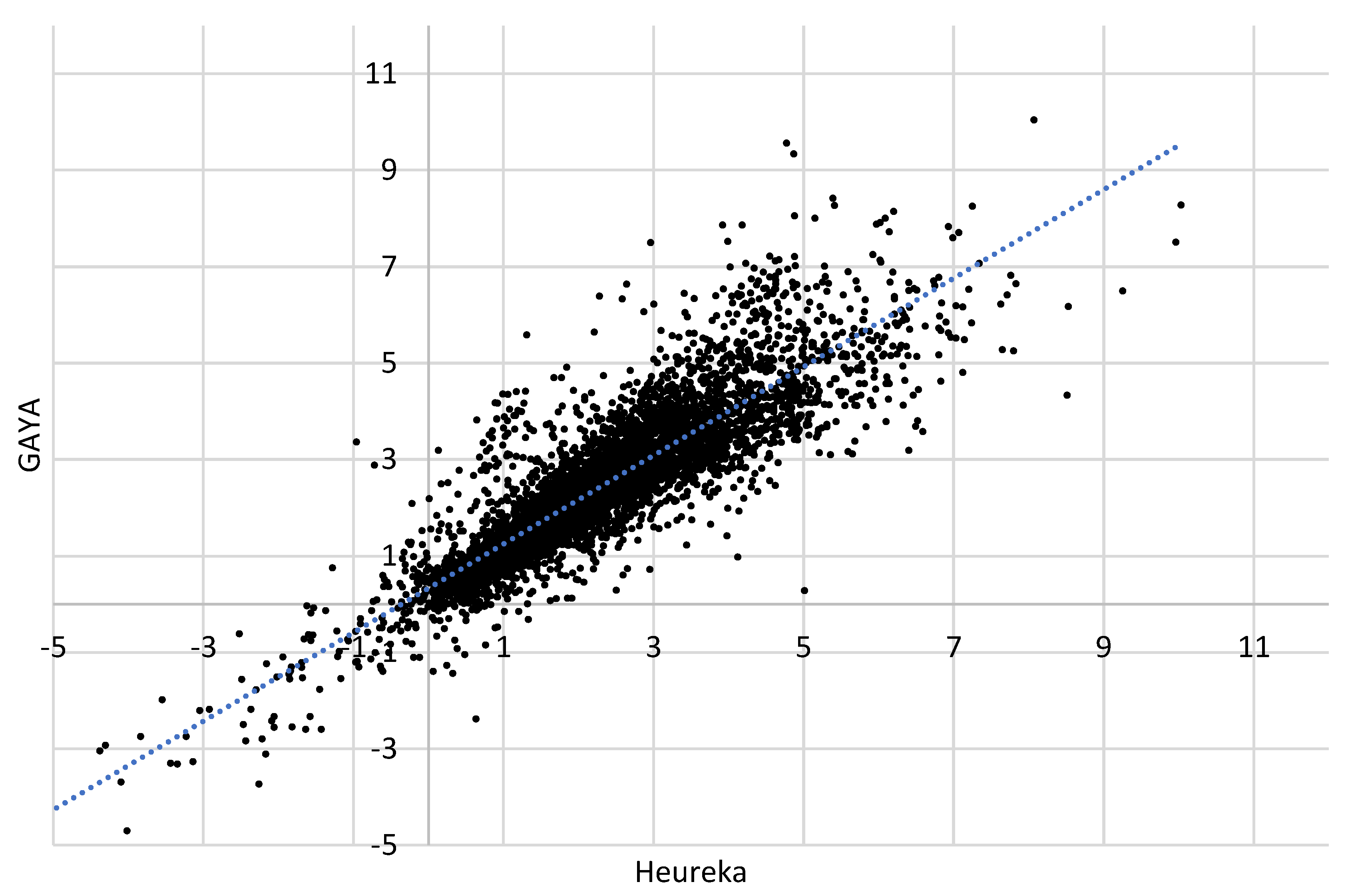
This comparison concerns 6294 NFI plots from the years 2016–2018 on productive forest land with basal area greater than 10 m2, height greater than 10 m, and less than 5000 stems ha−1 to limit the comparison to established forest. No breeding or climate change effects are included in order to compare the outcome of the most basic dynamic element of the systems, i.e., the basal area growth model, together with ingrowth and natural mortality. The Heureka system uses the calipered stem data on the NFI plots, whereas GAYA uses the corresponding average plot data.
The basal area growth is on the same level for both systems (2.13 and 2.29 m2 for 5 years with GAYA and Heureka, respectively) and with mean absolute error (MAE) of 0.49 m2 y−1, about 17% (Figure 3). The variation between Heureka and GAYA could have something to do with Heureka using stem data and GAYA plot averages; however, different assumptions of whether a plot is recently thinned or not could also be a source of the deviation.
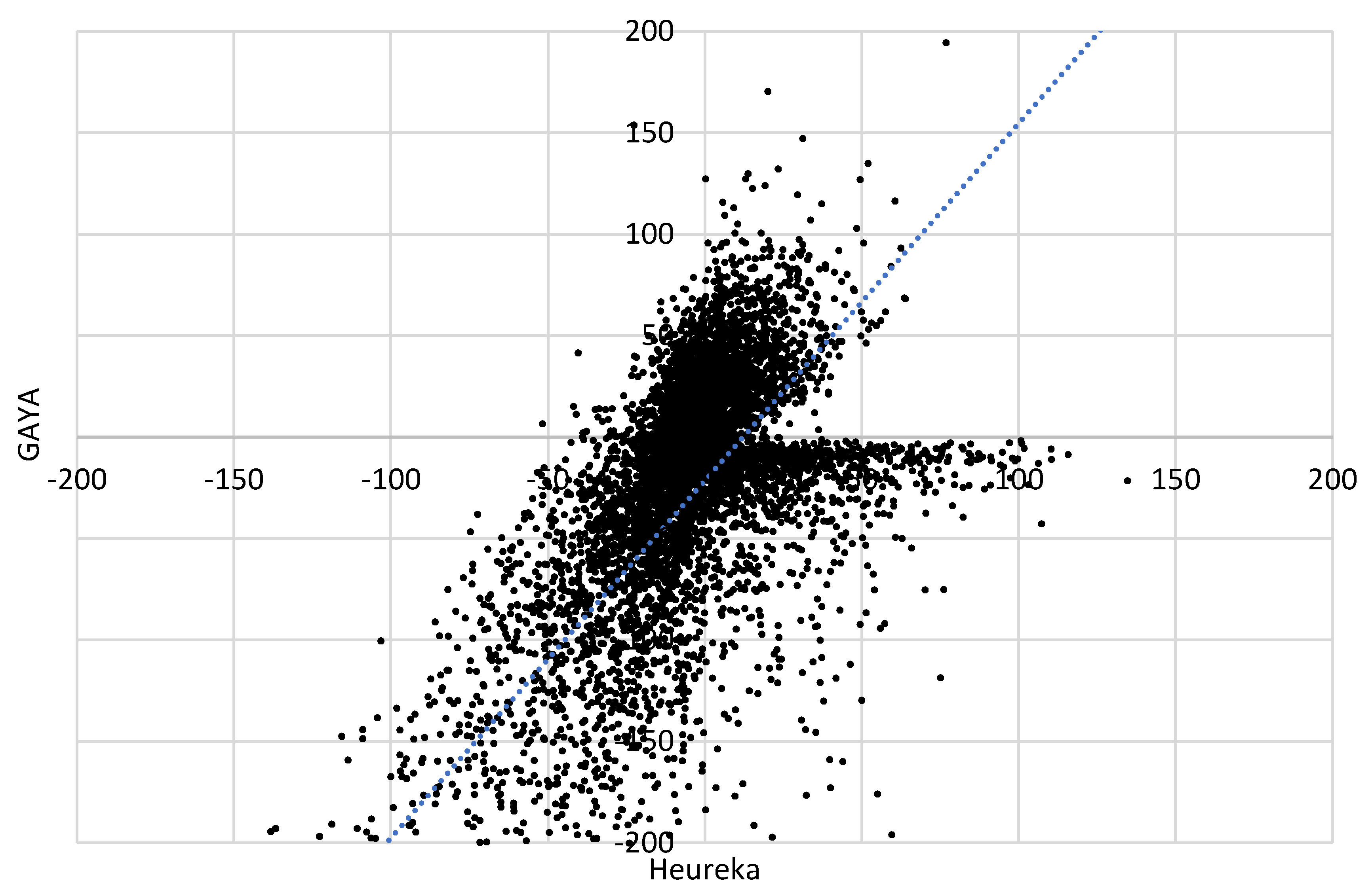
Another source of the deviation between GAYA and Heureka is ingrowth and mortality calculation. Comparison of the development of stems for the same period indicates that this might indeed be the case (Figure 4). It shows that there is a tendency for Heureka to have larger changes of stems than GAYA, i.e., ingrowth as well as mortality is greater. The average change of stems for GAYA is −6 stems and for Heureka it is −33 stems. Part of the difference could be attributed to those plots where GAYA has an increase of about 25 to 100 stems ha−1 and Heureka has no increase, creating a kind of gap in the diagram for which there is no obvious explanation.
3.2. Multi-Period Growth Comparison
A solution with a revised version of the forest sector model SweFor [24] that is supplied with forest management programmes from GAYA is compared with a solution by Heureka for a 100-year projection period. To make the solutions comparable, both models maximize net present value with a discount rate of 3%, and the total thinning volume and the volume from final harvests for each period of the SweFor solution are required to be the same in the Heureka solution. Both systems use 12,506 NFI plots from year 2017 and 2018 to describe the initial state of the Swedish forest. The management programs of Heureka are calculated with default values. Both solutions include the effect of tree breeding, whereas climate change is zeroed due to different implementations giving rise to different solutions.
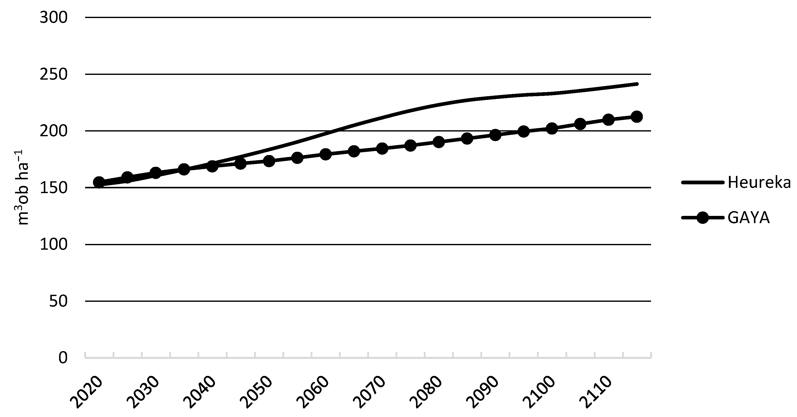
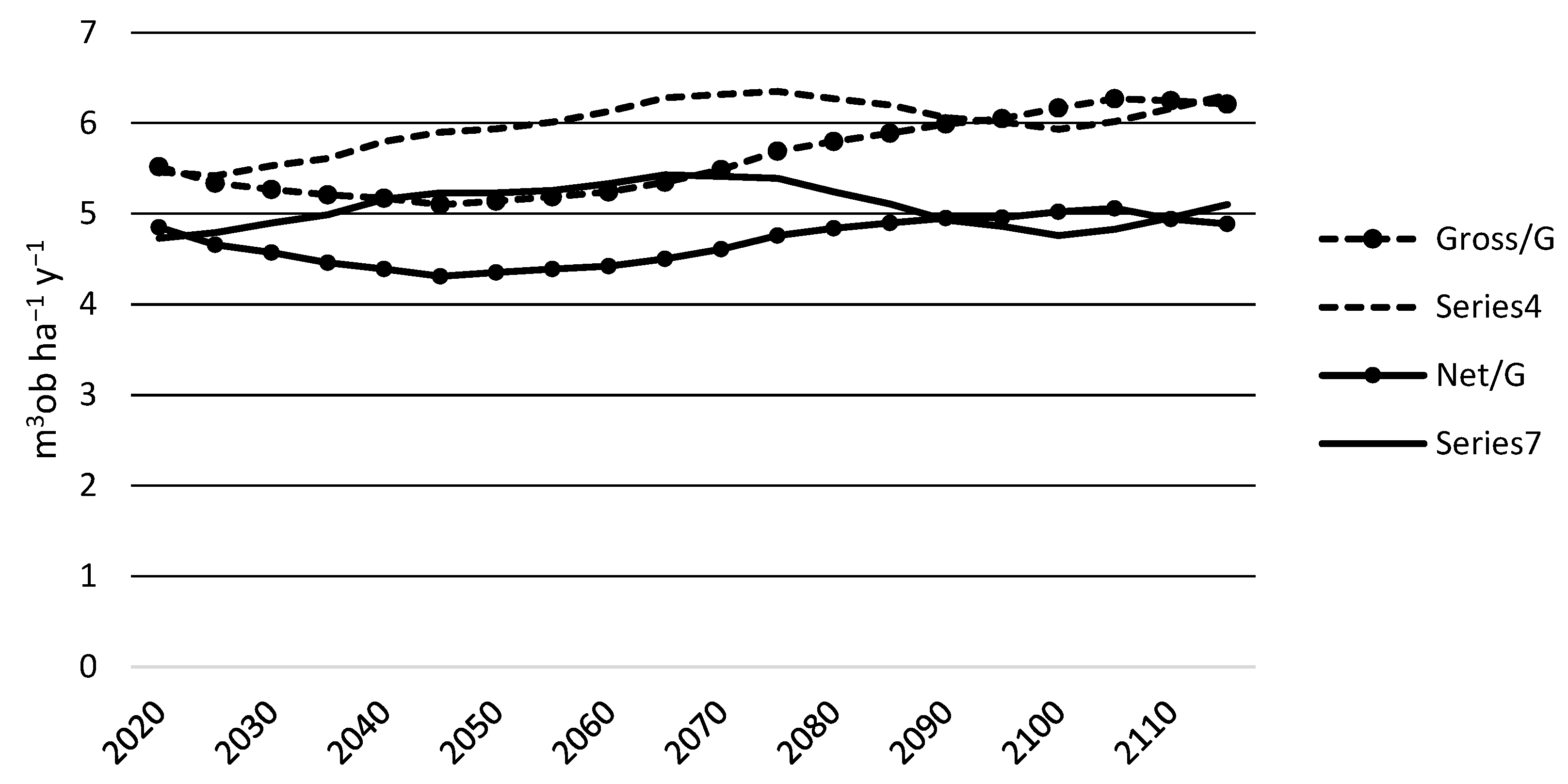
The stocking level is almost the same until 2045 (Figure 5). From that point it increases more rapidly for Heureka than for GAYA. It is reflected in the growth rate (Figure 6). From 2040, the Heureka increment takes a step up, whereas GAYA continues on almost the same level. Mortality is very stable over the projection period and is slightly lower for Heureka than for GAYA, on average 0.70 m3ob ha−1 y−1 for Heureka compared with 0.77 for GAYA. Comparing the first period gross increment with NFI data—5.2 m3ob ha−1 y−1—Heureka and GAYA are slightly above, 5.5 m3ob ha−1 y−1.
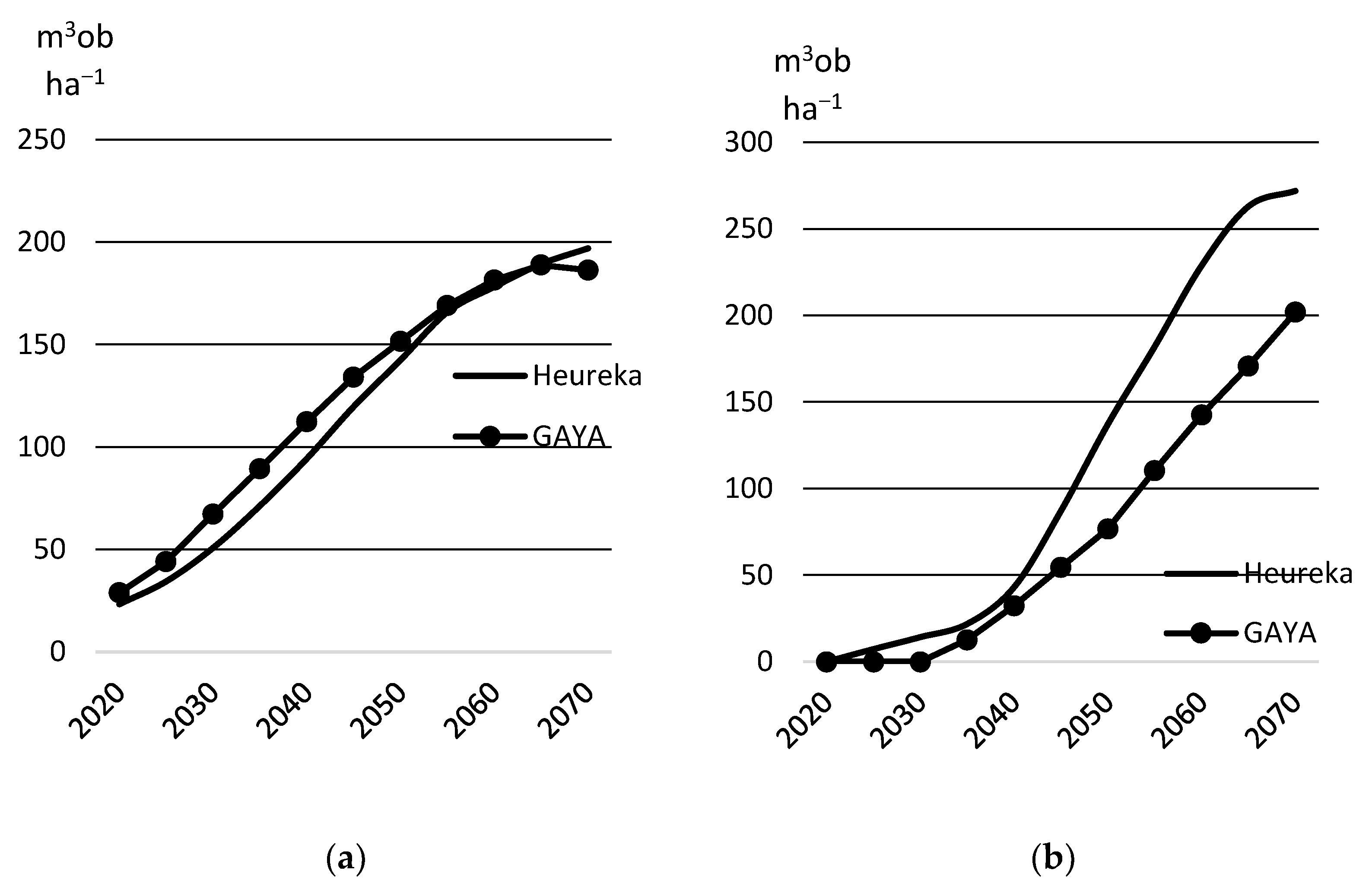
The reason for the increased growth rate from 2040 onwards should not be connected with the prediction of growth for established forest (see Figure 3). It is thus either residing with forest that is young or forest that is, or becomes, barren. The average stocking level for plots for which the initial state is classified as young—4.9 million ha with Heureka and 5.6 million ha with GAYA—is indicating a slightly better growth for GAYA than Heureka for the first 50 years (Figure 7a). The difference in growth rate is associated with forest that is regenerated on barren land. Figure 7b describes the development of forest that is clear cut in period one—816,000 ha with Heureka and 1,370,000 ha with GAYA. The average increase in volume during the 6th period after clear cut is with Heureka more than double of that to GAYA, 10.0 compared to 4.4 m3ob ha−1 y−1. The average volume in period 7, i.e., after 30 years after clear cut, is 137 m3ob ha−1 with Heureka and 77 with GAYA. The average volume for NFI material covering years 2014–2018 is 100 m3ob ha−1 for plots with volume weighted age between 25 and 35 years. This could indicate that growth of forest established on barren land is too low with GAYA.
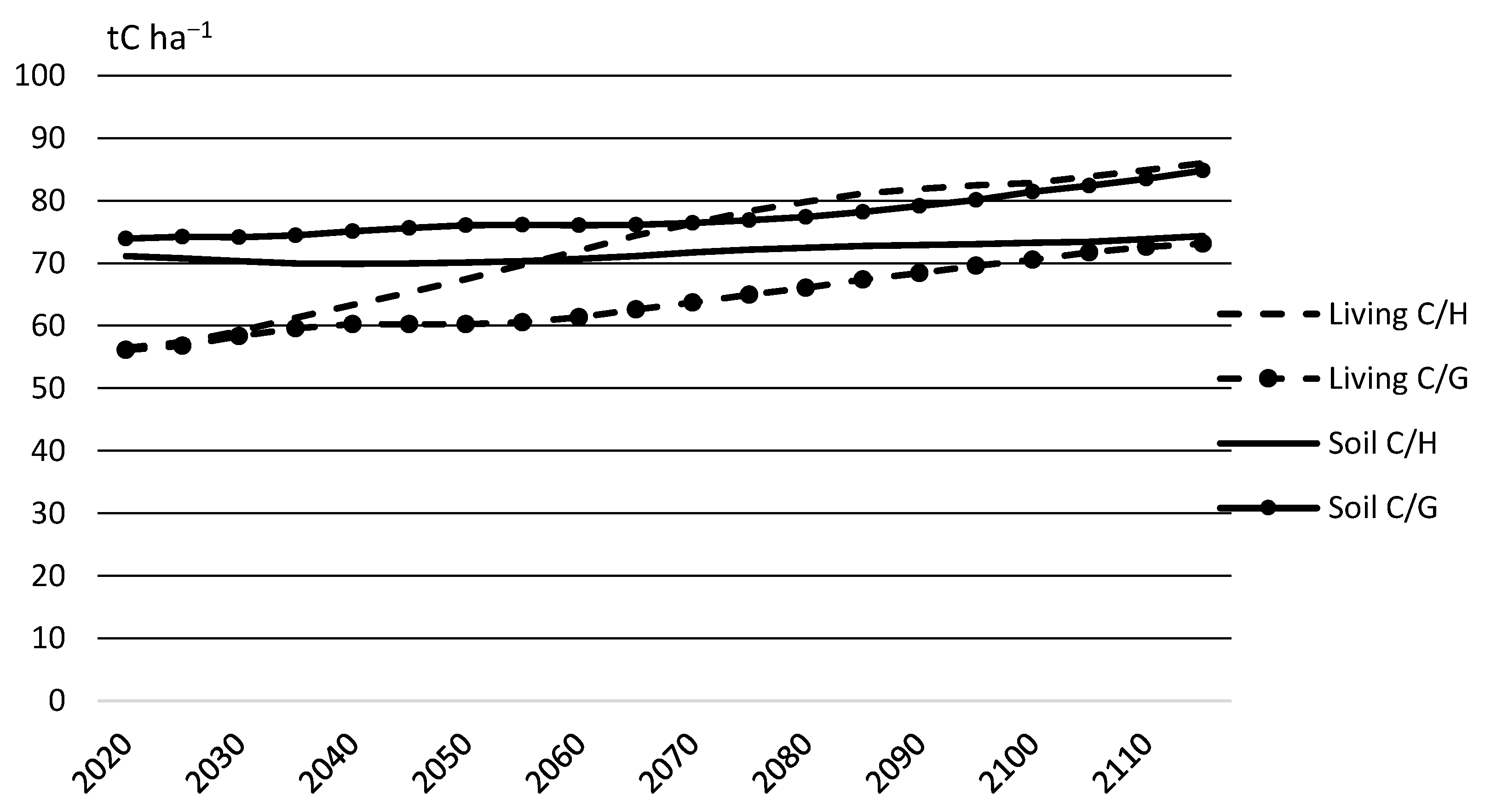
The investigation of carbon pools only includes mineral soils for reasons given above. The initial stocks of carbon of living matter are almost at the same value (Figure 8). Values in both cases are calculated on plot data, indicating that the functions for biomass are applied in a similar way. The development of carbon in living matter closely follows the amounts of standing volume. Soil carbon, i.e., all carbon except for carbon in living matter, is almost on the same level initially but deviates over time, i.e., with GAYA increases the amount whereas it stays on the same value with Heureka.
4. Discussion
The purpose of this paper is to present an implementation of GAYA that meets the standards of a reliable and scientifically based tool for generating management programmes. To help achieve that aim, the performance of GAYA is compared with the Heureka system, which in effect represents the industry standard in Sweden.
Apart from the first 5-year period, Heureka has a higher growth rate than GAYA for most of the projection period (see Figure 6). The difference should not pertain neither to established forest—the basal area growth for the population is the same, although with a deviation of close to 20% (see Figure 3)—nor the development of young forest (see Figure 7a). What differs between the two models is the establishment on barren land and the following projection of the establishment phase where Heureka predicts substantially higher growth than GAYA. As the new forest starts growing at a higher pace it boosts the growth rate of the entire forest (see Figure 6) and eventually in a stocking level becoming higher with Heureka than GAYA (see Figure 5). Compared to the current state of young forest, according to NFI data, there are indications that GAYA results in too low growth. The carbon in living matter is the same for both models if account is taken to the difference in standing volume. This should be the case since the calculations are made in the same way with the same functions. The simplified soil carbon model gives decay rates of the same magnitude as the more advanced models such as the Q model [51]. The increase calculated by GAYA, 110 kg C ha−1 y−1 over the projection period, would be in line with the 150 kg C ha−1 y−1 indicated in [63] and the general expectation of a continued increase [64].
Heureka offers many advantages that are far beyond what GAYA can provide. Heureka encompasses a range of different applications for different purposes, integrates a SQL database that makes modelling and results presentation within the system easy, and it is equipped with a developed GUI. It is ideal for the more advanced users among practising foresters. However, GAYA can offer comparative advantages for certain types of analyses. In particular, it offers a complete enumeration of management programmes ensures that, with a proper set of rules for permissible treatments, the decision domain is covered. With the arrangement documented in this study GAYA can churn out ca 1 million management programmes covering 100 years within five minutes on an ordinary laptop. This amount of management programs takes days to produce with Heureka.
Transparency and control could be given as arguments for the methods for non-established forest. GAYA gives the possibility to step over the contingencies associated with the establishment on barren land by inputting a young forest as an alternative to the (hitherto unpublished) modelling framework implemented in Heureka. It is possible that in this way the user of GAYA has more flexibility than with Heureka to test hypotheses developed in other models. This argument could be applied to the simplified climate change model as well. What the effects of climate change will be is, in the end, a choice made by the user based on assumptions of global mitigation strategies in combination with any of the various impacts of climate change offered by current research. With that in mind, a simple and transparent model may more easily lend itself to communication with interested target groups.
The most compelling argument for maintaining two systems within the same domain is perhaps that they can support each other’s development. Giving a reliable description of the development of a stand, a stand that could be located anywhere in the country in almost any condition and subject to any of a range of management interventions, is a complex matter. To analyse different outcomes and share the possible implementations of new scientific results should be the aim of both systems.
This article presents a particular implementation of GAYA. It represents the first comprehensive documentation of a projection system specifically adapted to Swedish conditions since the presentation of FMPP [25]. Reprogramming of the basic (administrative) functions of GAYA to C# is currently under way to allow for easier transferability to locations with other growth and yield conditions.
Author Contributions
J.B. provided the resources and methodology, and conducted the formal analyses and writing associated with the section ‘climate change growth effect’. L.O.E. provided the resources and methodology, and conducted the formal analyses, validation and writing for other parts of the manuscript. J.B. and L.O.E. planned the original draft together as well as the content of the discussion. All authors have read and agreed to the published version of the manuscript.
Funding
The research was funded by the Swedish Energy Agency (Energimyndigheten), Sweden, Project no. 2019-002673.
Data Availability Statement
The original description of the structure and content of the GAYA software is found in [30]. The program running the benchmark is downloaded from https://www.heurekaslu.se/wiki/Download_and_install/sv (accessed on 10 April 2022) where instructions for installation and running the model are found.
Acknowledgments
Assistance was received from several colleagues at the department of forest resource management, SLU, to help with data retrieval and implementation of different functions in GAYA. We would in particular like to mention Jeannette Eggers and Per-Erik Wikberg.
Conflicts of Interest
The authors declare no conflict of interest.
References
- Edenhofer, O.; Madruga, R.P.; Sokona, Y.; Seyboth, K.; Matschoss, P.; Kadner, S.; Zwickel, T.; Eickemeier, P.; Hansen, G.; Schlömer, S.; et al. Renewable Energy Sources and Climate Change Mitigation: Special Report of the Intergovernmental Panel on Climate Change; Cambridge University Press: Cambridge, UK, 2011; pp. 1–1075. [Google Scholar]
- European Commission. Fit for 55—Delivering the EU’s 2030 Climate Target on the Way to Climate Neutrality; European Commission: Brussels, Belgium, 2021; Available online: https://ec.europa.eu/info/publications/eu-communication-2019-stepping-eu-action-protect-and-restore-worlds-forests_en (accessed on 24 February 2022).
- FOREST EUROPE FOREST EUROPE Work Programme. 2016. Available online: https://foresteurope.org/wp-content/uploads/2016/08/FE-Work-Programme-2016-2020-1.pdf (accessed on 24 February 2022).
- Borges, J.G.; Nordström, E.-M.; Garcia Gonzalo, J.; Hujala, T.; Trasobares, A. Computer-Based Tools for Supporting Forest Management; SLU: Umeå, Sweden, 2014; Available online: https://pub.epsilon.slu.se/11417/ (accessed on 24 February 2022).
- Sallnäs, O.; Eriksson, L.O. Management Variation and Price Expectations in an Intertemporal Forest Sector Model. Nat. Resour. Model. 1989, 3, 385–398. [Google Scholar] [CrossRef]
- Schelhaas, M.-J.; Eggers, J.; Lindner, M.; Nabuurs, G.-J.; Pussinen, A.; Paivinen, R.; Schuck, A.; Verkerk, P.; Van der Werf, D.; Zudin, S. Model Documentation for the European Forest Information Scenario Model (EFISCEN 3.1.3); Alterra: Wageningen, The Netherlands, 2007; Available online: https://library.wur.nl/WebQuery/wurpubs/358645 (accessed on 24 February 2022).
- Mondal, P.; Southworth, J. Evaluation of Conservation Interventions Using a Cellular Automata-Markov Model. For. Ecol. Manag. 2010, 260, 1716–1725. [Google Scholar] [CrossRef]
- Salehi, A.; Eriksson, L.O. A Management Model for Persian Oak-A Model for Management of Mixed Coppice Stands of Semiarid Forests of Persian Oak. Math. Comput. For. Nat. Resour. Sci. 2010, 2, 20–29. [Google Scholar]
- Packalen, T.; Marques, A.; Rasinmäki, J.; Rosset, C.; Mounir, F.; Rodriguez, L.; Nobre, S. A Brief Overview of Forest Management Decision Support Systems (FMDSS) Listed in the FORSYS Wiki. For. Syst. 2013, 22, 263–269. [Google Scholar] [CrossRef] [Green Version]
- Härkönen, S.; Neumann, M.; Mues, V.; Berninger, F.; Bronisz, K.; Cardellini, G.; Chirici, G.; Hasenauer, H.; Koehl, M.; Lang, M.; et al. A Climate-Sensitive Forest Model for Assessing Impacts of Forest Management in Europe. Environ. Model. Softw. 2019, 115, 128–143. [Google Scholar] [CrossRef]
- Schwaiger, F.; Poschenrieder, W.; Biber, P.; Pretzsch, H. Ecosystem Service Trade-Offs for Adaptive Forest Management. Ecosyst. Serv. 2019, 39, 100993. [Google Scholar] [CrossRef]
- Goude, M.; Nilsson, U.; Mason, E.; Vico, G. Using Hybrid Modelling to Predict Basal Area and Evaluate Effects of Climate Change on Growth of Norway Spruce and Scots Pine Stands. Scand. J. For. Res. 2022, 37, 1–15. [Google Scholar] [CrossRef]
- Komarov, A.; Chertov, O.; Zudin, S.; Nadporozhskaya, M.; Mikhailov, A.; Bykhovets, S.; Zudina, E.; Zoubkova, E. EFIMOD 2—a Model of Growth and Cycling of Elements in Boreal Forest Ecosystems. Ecol. Model. 2003, 170, 373–392. [Google Scholar] [CrossRef]
- Wikström, P.; Edenius, L.; Elfving, B.; Eriksson, L.O.; Lämås, T.; Sonesson, J.; Öhman, K.; Wallerman, J.; Waller, C.; Klintebäck, F. The Heureka Forestry Decision Support System: An Overview. Math. Comput. For. Nat. Resour. Sci. 2011, 3, 87–94. [Google Scholar]
- Petrauskas, E.; Kuliešis, A. Scenario-Based Analysis of Possible Management Alternatives for Lithuanian Forests in the 21st Century. Balt. For. 2004, 10, 72–82. [Google Scholar]
- Fabrika, M. Modelling of Forest Production at Climate Change by Growth Model SIBYLA. In Proceedings of the Bioclimatology and Natural Hazards International Scientific Conference, Pol’ana nad Detvou, Slovakia, 17–20 September 2007; pp. 17–20. [Google Scholar]
- Pretzsch, H. Application and Evaluation of the Growth Simulator SILVA 2.2 for Forest Stands, Forest Estates and Large Regions. Forstwiss. Cent. 2002, 121, 28–51. [Google Scholar]
- Johnson, K.N.; Scheurman, H.L. Techniques for Prescribing Optimal Timber Harvest and Investment under Different Objectives—Discussion and Synthesis. For. Sci. 1977, 23, a0001–z0001. [Google Scholar]
- Hirvelä, H.; Härkönen, K.; Lempinen, R. MELA2016 Reference Manual; Luke: Helsinki, Finland, 2017; Available online: https://jukuri.luke.fi/bitstream/handle/10024/538149/luke-luobio_7_2017.pdf?sequence=6 (accessed on 24 February 2022).
- Pukkala, T. Dealing with Ecological Objectives in the Monsu Planning System. Silva. Lusit. 2004, 12, 1–15. [Google Scholar]
- Borges, J.G.; Falcao, A.O.; Miragaia, C.; Marques, P.; Marques, M. A Decision Support System for Forest Ecosystem Management in Portugal. In Systems Analysis in Forest Resources; Springer: Berlin/Heidelberg, Germany, 2003; pp. 155–163. [Google Scholar]
- Alig, R.J.; Adams, D.M.; McCarl, B.A. Impacts of Incorporating Land Exchanges between Forestry and Agriculture in Sector Models. J. Agric. Appl. Econ. 1998, 30, 389–401. [Google Scholar] [CrossRef] [Green Version]
- Sjølie, H.K.; Latta, G.S.; Gobakken, T.; Solberg, B. NorFor: A Forest Sector Model of Norway: Model Overview and Structure; MINA Fagrapport 18; INA: Aas, Norway, 2011; Available online: https://hdl.handle.net/11250/2647392 (accessed on 24 February 2022).
- Eriksson, L.O.; Forsell, N.; Eggers, J.; Snäll, T. Downscaling of Long-Term Global Scenarios to Regions with a Forest Sector Model. Forests 2020, 11, 500. [Google Scholar] [CrossRef]
- Jonsson, B.; Jacobsson, J.; Kallur, H. The forest management planning package: Theory and application. Studia For. Suec. 1993, 183, 1–56. [Google Scholar]
- Lundström, A.; Söderberg, U. Outline of the Hugin System for Long-Term Forecasts of Timber Yields and Possible Cut-Introduction. In Proceedings of the Large-Scale Forestry Scenario Models: Experiences and Requirements, Joensuu, Finland, 15–22 June 1995; Volume 5, pp. 63–77. [Google Scholar]
- Nilsson, P.; Roberge, C.; Fridman, J. Skogsdata 2021: Aktuella Uppgifter om de Svenska Skogarna Från SLU Riksskogstaxeringen; SLU Institutionen för Skoglig Resurshushållning: Umeå, Sweden, 2021; Available online: https://www.slu.se/globalassets/ew/org/centrb/rt/dokument/skogsdata/skogsdata_2021_webb.pdf (accessed on 24 February 2022).
- Heureka Publications. Available online: https://www.slu.se/en/departments/forest-resource-management/program-project/forest-sustainability-analysis/sha/publications/ (accessed on 24 February 2022).
- Eriksson, L.O. Timber Class Formation by Cluster Analysis; Department of Forest Technology, Swedish University of Agricultural Sciences: Garpenberg, Sweden, 1983. [Google Scholar]
- Hoen, H.F.; Eid, T. En Modell for Analyse Av Behandlingsstrategier for En Skog Ved Bestandssimulering Og Lineær Programmering [A Model for Analysis of Treatment Strategies for a Forest by Stand Simulation and Linear Programming]; Norsk Institutt for Skogforskning–NISK: Ås, Norway, 1990. [Google Scholar]
- Eriksson, L.O.; Lofgren, S.; Ohman, K. Implications for Forest Management of the EU Water Framework Directive’s Stream Water Quality Requirements-A Modeling Approach. For. Policy Econ. 2011, 13, 284–291. [Google Scholar] [CrossRef]
- Borges, P.; Eid, T.; Bergseng, E. Applying Simulated Annealing Using Different Methods for the Neighborhood Search in Forest Planning Problems. Eur. J. Oper. Res. 2014, 233, 700–710. [Google Scholar] [CrossRef]
- Ezzati, S.; Palma, C.D.; Bettinger, P.; Eriksson, L.O.; Awasthi, A. An Integrated Multi-Criteria Decision Analysis and Optimization Modeling Approach to Spatially Operational Road Repair Decisions. Can. J. For. Res. 2021, 51, 465–483. [Google Scholar] [CrossRef]
- Hägglund, B. Om Övre Höjdens Utveckling För Gran i Norra Sverige. Skogshögskolan, Institutionen För Skogsproduktion. Rapp. Och Uppsats. 1972, 21, 298. [Google Scholar]
- Hägglund, B. Om Övre Höjdens Utveckling För Gran i Södra Sverige. Skogshögskolan, Institutionen För Skogsproduktion. Rapp. Och Uppsats. 1973, 24, 49. [Google Scholar]
- Hägglund, B. Övre Höjdens Utveckling i Tallbestånd. Skogshögskolan, Institutionen För Skogsproduktion. Rapp. Och Uppsats. 1974, 31, 54. [Google Scholar]
- Pettersson, N. The Effect of Density after Precommercial Thinning on Volume and Structure in Pinus sylvestris and Picea Abies Stands. Scand. J. For. Res. 1993, 8, 528–539. [Google Scholar] [CrossRef]
- Elfving, B. Growth Modelling in the Heureka System; Swedish University of Agricultural Sciences: Umeå, Sweden, 2010. [Google Scholar]
- Fahlvik, N.; Elfving, B.; Wikström, P. Evaluation of Growth Functions Used in the Swedish Forest Planning System Heureka. Silva. Fenn. 2014, 48, 1013. [Google Scholar] [CrossRef] [Green Version]
- Haapanen, M.; Jansson, G.; Nielsen, U.B.; Steffenrem, A.; Stener, L.G. The status of Tree Breeding and Its Potential for Improving Biomass Production—A Review of Breeding Activities and Genetic Gains in Scandinavia and Finland; Skogforsk: Uppsala, Sweden, 2015; Available online: https://www.skogforsk.se/contentassets/9d9c6eeaef374a2283b2716edd8d552e/the-status-of-tree-breeding-low.pdf (accessed on 24 February 2022).
- Söderberg, U. Funktioner För Skogliga Produktionsprognoser. SLU, Avd. För Skogsuppskattning Och Skogsindelning. Rapport 14; SLU: Umeå, Sweden, 1986. [Google Scholar]
- Bengtsson, G. Beräkning Av Den Naturliga Avgången i Avverkningsberäkningarna För 1973 Års Skogsutrednings Slutbetänkande; Skog För Framtid, SOU 1978:7, Bilaga 6; Näringsdepartementet: Stockholm, Sweden, 1978; Available online: https://weburn.kb.se/metadata/907/SOU_7258907.htm (accessed on 24 February 2022).
- Wikberg, P.-E. Occurence, Morphology and Growth of Understory Saplings in Swedish Forests; Acta Universitatis Agriculturae Sueciae Silvestria; Swedish University of Agricultural Sciences: Umeå, Sweden, 2004. [Google Scholar]
- Pettersson, F. Predictive Functions for Impact of Nitrogen Fertilization on Growth over Five Years. For. Res. Inst. Swed. 1994. Available online: https://www.osti.gov/etdeweb/biblio/6892928 (accessed on 24 February 2022).
- Agestam, E. En Produktionsmodell för Blandbestånd Av Tall, Spruce Och Björk I Sverige [A Growth Simulator for Mixed Stands of Pine, Spruce and Birch in Sweden]; Institutionen för Skogsproduktion, Sveriges Lantbruksuniversitet: Garpenberg, Sweden, 1985. [Google Scholar]
- Hagberg, E.; Matérn, B. Volymfunktioner För Stående Träd Av Ek Och Bok: Materialet Och Dess Bearbetning = Tree Volume Functions for Oak and Beech in Sweden (Quercus Robur and Fagus Silvatica); Rapporter Och Uppsatser/Institutionen för Skoglig Matematisk Statistik, Skogshögskolan, 15: Stockholm, Sweden, 1975. [Google Scholar]
- Brandel, G. Volymfunktioner För Enskilda Träd: Tall, Gran Och Björk = Volume Functions for Individual Trees: Scots Pine (Pinus sylvestris), Norway Spruce (Picea Abies) and Birch (Betula Pendula & Betula Pubescens); Sveriges Lantbruksuniv: Garpenberg, Sweden, 1990. [Google Scholar]
- Kjellström, E.; Bärring, L.; Gollvik, S.; Hansson, U.; Jones, C.; Samuelsson, P.; Ullerstig, A.; Willén, U.; Wyser, K. A 140-Year Simulation of European Climate with the New Version of the Rossby Centre Regional Atmospheric Climate Model. (RCA3); SMHI: Norrköping, Sweden, 2005. [Google Scholar]
- Nakicenovic, N.; Swart, R. Emissions Scenarios-Special Report of the Intergovernmental Panel on Climate Change. In Intergovernmental Panel on Climate Change Special Reports on Climate Change; Cambridge University Press: Cambridge, UK, 2000; p. 570. [Google Scholar]
- Bergh, J.; Blennow, K.; Nilsson, U.; Sallnäs, O. Effekter Av Ett Förändrat Klimat På Skogen (Effects of a Changing Climate on the Forest); Department of Southern Swedish Forest Research Centre, SLU: Alnarp, Sweden, 2007. [Google Scholar]
- Ågren, G.I.; Bosatta, E. Theoretical Ecosystem Ecology: Understanding Element Cycles; Cambridge University Press: Cambridge, UK, 1998. [Google Scholar]
- Viskari, T.; Laine, M.; Kulmala, L.; Mäkelä, J.; Fer, I.; Liski, J. Improving Yasso15 Soil Carbon Model Estimates with Ensemble Adjustment Kalman Filter State Data Assimilation. Geosci. Model. Dev. 2020, 13, 5959–5971. [Google Scholar] [CrossRef]
- Petersson, H. Biomassafunktioner För Trädfaktorer Av Tall, Gran Och Björk i Sverige; Institutionen för Skoglig Resurshushållning, Sveriges Lantbruksuniversitet: Umeå, Sweden, 1999. [Google Scholar]
- Ollas, R. Nya Utbytesfunktioner För Träd Och Bestånd [New Yield Functions for Trees and Stands], Ekonomi, 5; Forskningsstiftelsen Skogsarbeten: Stockholm, Sweden, 1980; p. 20. [Google Scholar]
- Starr, M.; Saarsalmi, A.; Hokkanen, T.; Merilä, P.; Helmisaari, H.-S. Models of Litterfall Production for Scots Pine (Pinus sylvestris L.) in Finland Using Stand, Site and Climate Factors. For. Ecol. Manag. 2005, 205, 215–225. [Google Scholar] [CrossRef]
- Saarsalmi, A.; Starr, M.; Hokkanen, T.; Ukonmaanaho, L.; Kukkola, M.; Nöjd, P.; Sievänen, R. Predicting Annual Canopy Litterfall Production for Norway Spruce (Picea Abies (L.) Karst.) Stands. For. Ecol. Manag. 2007, 242, 578–586. [Google Scholar] [CrossRef]
- Eriksson, E.; Gillespie, A.R.; Gustavsson, L.; Langvall, O.; Olsson, M.; Sathre, R.; Stendahl, J. Integrated Carbon Analysis of Forest Management Practices and Wood Substitution. Can. J. For. Res. 2007, 37, 671–681. [Google Scholar] [CrossRef]
- Berg, B.; Meentemeyer, V. Litter Fall in Some European Coniferous Forests as Dependent on Climate: A Synthesis. Can. J. For. Res. 2001, 31, 292–301. [Google Scholar] [CrossRef]
- Eriksson, B. Den «Potentiella» Evapotranspirationen i Sverige [The «Potential» Evapotranspiration in Sweden]; SMHI: Norrköping, Sweden, 1981; Available online: http://smhi.diva-portal.org/smash/get/diva2:1462578/FULLTEXT01.pdf (accessed on 24 February 2022).
- Eriksson, A.; Westerlund, B.; Dahlgren, J.; Fridman, J.; Claesson, S.; Wulff, S. Global Forest Resources Assessment 2020 Report; FAO: Rome, Italy, 2020; Available online: https://www.fao.org/3/cb0063en/cb0063en.pdf (accessed on 24 February 2022).
- Ortiz, C.; Karltun, E.; Stendahl, J.; Gärdenäs, A.I.; Ågren, G.I. Modelling Soil Carbon Development in Swedish Coniferous Forest Soils—An Uncertainty Analysis of Parameters and Model Estimates Using the GLUE Method. Ecol. Model. 2011, 222, 3020–3032. [Google Scholar] [CrossRef]
- Hyvönen, R.; Ågren, G.I. Decomposer Invasion Rate, Decomposer Growth Rate, and Substrate Chemical Quality: How They Influence Soil Organic Matter Turnover. Can. J. For. Res. 2001, 31, 1594–1601. [Google Scholar] [CrossRef]
- Bergh, J.; Egnell, G.; Lundmark, T. Skogens Kolbalans Och Klimatet; Skogsskötselserien; Skogsstyrelsen: Jönköping, Sweden, 2020. [Google Scholar]
- Ågren, G.I.; Hyvönen, R.; Nilsson, T. Are Swedish Forest Soils Sinks or Sources for CO2—Model Analyses Based on Forest Inventory Data. Biogeochemistry 2008, 89, 139–149. [Google Scholar] [CrossRef]
Figure 1.
The projection of one management programme. Controls entirely in the hands of the user are marked with thick borders of decision points.
Figure 1.
The projection of one management programme. Controls entirely in the hands of the user are marked with thick borders of decision points.

Figure 2.
Relative change of production (%) for B2 and A2 scenarios for spruce, pine, and deciduous species for the period 2015−2090: (a,b) refer to Norway spruce, (c,d) to Scots pine, (e,f) to deciduous species; (a,c,e) to climate scenario B2, and (b,d,f) to climate scenario A2; Northern Sweden (<59′ N), central (59−63′ N), and northern (>63′ N) Sweden.

Figure 3.
The net growth of established forest in basal area (m2 ha−1) for five years from current state, GAYA vs. Heureka, and trend line.
Figure 3.
The net growth of established forest in basal area (m2 ha−1) for five years from current state, GAYA vs. Heureka, and trend line.

Figure 4.
The change of number of stems ha−1 for five years from current state, GAYA vs. Heureka.

Figure 5.
Standing volume with Heureka and GAYA.

Figure 6.
The gross and net increment with GAYA (/G) and Heureka (/H).

Figure 7.
Mean standing volume for Heureka and GAYA for land whose initial state is classified as young (a) and mean standing volume for land that is clear cut during the first period (b).
Figure 7.
Mean standing volume for Heureka and GAYA for land whose initial state is classified as young (a) and mean standing volume for land that is clear cut during the first period (b).

Figure 8.
Pools of carbon in living matter and soil with GAYA (/G) and Heureka (/H).


Table 1.
Average form height of NFI plots years 2014–2018 in height interval 7–10 m (taking account of the difference between average height and dominant height).
Table 1.
Average form height of NFI plots years 2014–2018 in height interval 7–10 m (taking account of the difference between average height and dominant height).
| Pine | Spruce | Birch | As-Pen | Oak | Beech | Southern Broad-Leaves | Lodgepole Pine | Other Broad-Leaves | Larch |
|---|---|---|---|---|---|---|---|---|---|
| 4.64 | 4.59 | 4.21 | 3.89 | 4.09 | 3.96 | 4.28 | 4.62 | 4.16 | 4.09 |
Table 2.
Functions for relative change of production for B2 and A2 scenarios for different regions and species.
Table 2.
Functions for relative change of production for B2 and A2 scenarios for different regions and species.
| B2 | A2 | |||||
|---|---|---|---|---|---|---|
| Region | a | b | c | a | b | c |
| Spruce | ||||||
| Northern | −0.0021208 | 8.9515 | −9428 | −0.0096970 | 40.308 | −41,853 |
| Central | −0.0004543 | 2.2082 | −2607 | −0.0093939 | 38.946 | −40,338 |
| Southern | −0.0046969 | 19.841 | −20,914 | −0.0098485 | 40.747 | −42,122 |
| Pine | ||||||
| Northern | −0.0009089 | 3.9864 | −4344 | −0.0063640 | 26.501 | −27,560 |
| Central | −0.0018182 | 7.7127 | −8160 | −0.0054549 | 22.745 | −23,686 |
| Southern | −0.0040910 | 17.164 | −17,978 | −0.0053031 | 22.175 | −23,154 |
| Deciduous | ||||||
| Northern | −0.0010606 | 4.5724 | −4907 | −0.0018182 | 7.6894 | −8113 |
| Central | 0.0030304 | −12.215 | 12,309 | −0.0015152 | 6.4573 | −6861 |
| Southern | 0.0016667 | −6.4967 | 6322 | −0.0040913 | 17.234 | −18,118 |
Table 3.
The key to functions in [53] and the corresponding biomass component where T, G, and B are used for pine, spruce, and deciduous trees, respectively.
Table 3.
The key to functions in [53] and the corresponding biomass component where T, G, and B are used for pine, spruce, and deciduous trees, respectively.
| Component | Function Key |
|---|---|
| Stump and roots > 5 cm | GT9 |
| Total biomass | T16, G7 |
| Stem biomass | T10, G1, B18 |
| Total biomass above stump | T15, G6, B22 |
Publisher’s Note: MDPI stays neutral with regard to jurisdictional claims in published maps and institutional affiliations. |
© 2022 by the authors. Licensee MDPI, Basel, Switzerland. This article is an open access article distributed under the terms and conditions of the Creative Commons Attribution (CC BY) license (https://creativecommons.org/licenses/by/4.0/).
Share and Cite
MDPI and ACS Style
Eriksson, L.O.; Bergh, J. A Tool for Long-Term Forest Stand Projections of Swedish Forests. Forests 2022, 13, 816. https://0-doi-org.brum.beds.ac.uk/10.3390/f13060816
AMA Style
Eriksson LO, Bergh J. A Tool for Long-Term Forest Stand Projections of Swedish Forests. Forests. 2022; 13(6):816. https://0-doi-org.brum.beds.ac.uk/10.3390/f13060816
Chicago/Turabian StyleEriksson, Ljusk Ola, and Johan Bergh. 2022. "A Tool for Long-Term Forest Stand Projections of Swedish Forests" Forests 13, no. 6: 816. https://0-doi-org.brum.beds.ac.uk/10.3390/f13060816
Note that from the first issue of 2016, this journal uses article numbers instead of page numbers. See further details here.