A Photogrammetric Workflow for the Creation of a Forest Canopy Height Model from Small Unmanned Aerial System Imagery

Abstract

The recent development of operational small unmanned aerial systems (UASs) opens the door for their extensive use in forest mapping, as both the spatial and temporal resolution of UAS imagery better suit local-scale investigation than traditional remote sensing tools. This article focuses on the use of combined photogrammetry and “Structure from Motion” approaches in order to model the forest canopy surface from low-altitude aerial images. An original workflow, using the open source and free photogrammetric toolbox, MICMAC (acronym for Multi Image Matches for Auto Correlation Methods), was set up to create a digital canopy surface model of deciduous stands. In combination with a co-registered light detection and ranging (LiDAR) digital terrain model, the elevation of vegetation was determined, and the resulting hybrid photo/LiDAR canopy height model was compared to data from a LiDAR canopy height model and from forest inventory data. Linear regressions predicting dominant height and individual height from plot metrics and crown metrics showed that the photogrammetric canopy height model was of good quality for deciduous stands. Although photogrammetric reconstruction significantly smooths the canopy surface, the use of this workflow has the potential to take full advantage of the flexible revisit period of drones in order to refresh the LiDAR canopy height model and to collect dense multitemporal canopy height series.

1. Introduction

Unmanned Aerial Systems (UASs) are pre-programmed flying robots made up of an unmanned aerial vehicle (UAV) and a ground control system. UASs are now being designed for geomatic use and offer plenty of opportunities in the area of environmental sciences [1]. The spatial resolution of UAS imagery can reach a sub-decimeter ground sample distance (GSD), and the revisit period between two acquisitions can be selected in order to fit diverse scales of ecological phenomena. Small and lightweight UASs, in particular, are likely to become a versatile tool for scientists and environmentalists [2,3,4]. Along with this rising use of drones, dense three-dimensional reconstruction through the combined use of photogrammetry and “Structure from Motion” (SfM) state-of-the-art techniques has triggered the “come back of photogrammetry” [5]. Indeed, the ubiquitous use of numerical photography instead of analogical photography and the continuous improvements in computer computation power have turned digital photogrammetry into a viable surrogate for laser scanning [6]. The SfM algorithms originate from the field of computer vision and aim to automatically determine scene geometry, camera calibration, position and orientation from an unordered overlapping collection of images [7]. This results in a sparse 3D point cloud and camera orientations that are subsequently used for multi-view dense image-matching.

Low altitude UAS imagery may be used to observe forest canopy height [8,9]. Canopy height measurements are of great interest for the estimation of forest biomass and carbon stock [10,11], the monitoring of harvests and recruitment [12] and, more generally, in ecosystem process modeling. In the field of multi-source forest inventory, structural forest attributes are commonly extracted from the canopy height model by means of regression models predicting forest variables with metrics (i.e., descriptive statistic of the canopy height model on a particular area) [12,13]. The practical outcomes of canopy height models, in combination with field measurements, are the prediction of forest attributes of interest, such as stand density and maturity indicators. Light detection and ranging (LiDAR), also called airborne laser scanning (ALS) [14], is an active sensor that has been widely used in order to collect high resolution information on forest structure [15,16,17,18,19,20]. ALS data is acquired via the emission of laser pulses from an aerial platform (plane or helicopter) [21]. The emitted pulses can penetrate below the canopy and, thus, allow the recording of multiple returns, depending on the system. The result is a three-dimensional georeferenced point cloud, which can be very dense, depending on the flight characteristics. The ability of LiDAR to capture multiple returns and to reach the ground, even in forested areas, allows for the generation of a digital terrain model (DTM) and the estimation of forest variables [22,23]. Multi-source forest inventories on a national or regional scale can thus take full advantage of LiDAR data [13]. Only a small number of studies have shown that digital photogrammetry using spaceborne imagery or airborne imagery (acquired with manned airplanes) is also appropriate for the determination of forest canopy heights [24,25,26,27,28,29]. Compared to LiDAR, the main limitation of these methods is the impossibility of acquiring under-canopy information as a DTM [30]. Moreover, image matching in an area of vegetation is well known to be quite challenging, due to the numerous vegetation characteristics that hinder image matching: omissions, repetitive texture, multi-layered or moving objects [8,30,31]. The abrupt vertical changes occurring between the trees crowns and the microtopography of the canopy (characterized by high variations of the relief) cause multiple omissions that mar the dense-matching process. Nevertheless, these issues can be partly overcome, and previous investigations have shown that a photogrammetric digital canopy surface model may be generated by automatic image matching with an acceptable level of accuracy and resolution [32]. These photogrammetric digital surface models (photo-DSMs) can be advantageously combined with a DTM generated from topographic or LiDAR data in order to produce a hybrid photo-topo or photo-LiDAR canopy height model (this last model being designated in this paper under the acronym, photo-CHM). National level acquisitions of LiDAR scans have been completed in several European countries [27], thus providing accurate DTMs on large surfaces. Photogrammetry could be advantageously used to update LiDAR canopy height models and to constitute multi-temporal canopy height series. On a local scale, UAS imagery is characterized by a high image overlap and, thus, a high level of information redundancy. It therefore has the potential to accurately model the canopy surface at a very high spatial and temporal resolution. A similar approach has previously been investigated by Dandois and Ellis [9,33], by using kite and hobbyist-grade UAS imagery for the modeling of outer canopy height in a limited area, due to low altitude acquisitions (UAS at 40 m above the canopy cover). The authors of Tao et al. [34] used UAS imagery for dense point-cloud generation on a forested area in order to provide a cost-effective alternative to LiDAR acquisition. On the other hand, Wallace et al. [35] and Jaakkola et al. [36] worked with multi-sensor UAS platforms, consisting of a small UAS carrying both a camera and a lightweight LiDAR. These authors highlighted the potential of such platforms for inventories realized at the level of individual trees.

In this article, a small fixed-wing UAS was used to obtain forest low-altitude and low-oblique vantage images. The aircraft had a coverage area of approximately 200 ha with a ground sample distance (GSD) of 8 cm in a single flight. An open source piece of software, MICMAC, was used to process the image block in order to produce a high resolution photo-DSM. This photo-DSM was subsequently co-registered with a LiDAR-DTM. Finally, the photo-CHM was compared to a reference LiDAR-CHM. This study mainly aimed to develop a photogrammetric workflow suited to forest UAS imagery. In addition, recurring issues and major opportunities concerning the use of UAS photogrammetry in forested areas are identified and discussed. The assessment of forest density indicators from the UAS canopy height model, such as the volume per hectare, was not investigated further in this research. However, tests were carried out in order to determine how satisfactorily dominant height and individual height might be derived from photo-CHM. Models for estimating the dominant height of irregular deciduous stands from area-based metrics, extracted from the photo-CHM, were evaluated. Their performance was then compared to LiDAR-CHM regression models.

2. Material and Methods

2.1. Study Site and Field Measurements

The study area is located near the village of Felenne, in Belgium. The forest is made up of a mix of uneven-aged broadleaved stands with a predominance of oaks (Quercus robur L. and Quercus petraea (MATT) Liebl.) and some even-aged coniferous stands. The coniferous stands are mainly pure spruce stands (Picea abies (L.) Karst.), including, however, some mixed plantations of Douglas-fir (Pseudotsuga menziesii (Mirb.) Franco) and spruce. Hornbeam (Carpinus betulus L.) and birch (Betula pendula Roth. and Betula pubescens Ehrh.) are either scattered in bunches or stand alone in deciduous stands. The maturity and dominant height of the stands can vary considerably. As a consequence, the vertical structure and deep relief variability, as well as the canopy surface elevation show both local and large variations.

A forest inventory was carried out in autumn, 2012, in order to compare digital canopy height models with field measurements. The forest inventory used variable-area circular plots installed on a systematic 150 × 150 m grid and focused exclusively on deciduous stands. The plot radius was adapted to keep to a minimum number of 20 trees. A maximum plot radius was fixed at 18 m (10 ares) in the case of low tree density. The following observations were recorded for each tree: circumference at breast height (CBH; measured at 130 cm), species, distance and azimuth from the plot center. Plot position was established using an SXBlue II differential GPS with an accuracy of a few meters under the canopy. For each plot, dominant height was calculated as the average of dominant tree heights, which have to be representative of the 100 tallest trees per hectare. The number of dominant trees measured varied for each plot and corresponded to the number of the plot area plus 1 (e.g., 11 dominant trees were measured on a plot of 10 ares). Dominant trees were determined according to their largest CBH, and their height was measured using a Haglöf Vertex laser hypsometer (Vertex IV). This methodology for forest inventory enables the estimation of stand dominant height and other dendrometric indicators with high density variations, while keeping an almost constant inventory effort for each plot [37]. In total, 36 plots located in irregular deciduous stands were inventoried.

In addition to plot inventory, complementary measurements of individual tree height were made for dominant deciduous trees spread around the study site. Attention was paid to measuring a wide range of tree heights. Four height measurements were made for each tree from different vantages in order to improve the level of measurement accuracy, which is approximately 0.5 m, according to [38]. Tree heights were computed as the average of these measurements. Tree crowns associated with field measurements were identified on CHMs and were manually delineated.

2.2. Unmanned Aerial System Survey

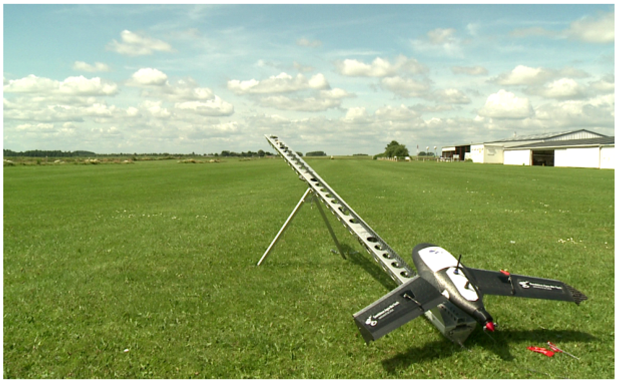
2.2.1. Small UAS Platform and the Sensor Used in the Present Study

The Gatewing X100 small UAS [39] (wingspan: 100 cm; weight: 2 kg; cruise speed: 80 km/h; flight height: from 100 m to 750 m; maximum flight duration: 40 min) was chosen for its ability to cover a relatively large area in a single flight. This UAS is equipped with an inertial measurement unit (IMU) and a GPS. These sensors determine the position, as well as the altitude of the X100 during the flight. It should, however be pointed out that the GPS accuracy is approximately a few meters, and the orientation angle (yaw, pitch, roll) accuracy is about 2 degrees. The UAS flight plan is prepared using a specific software designed for the X100 (Quickfield^®). A ground control station (GCS) records the flight characteristics (working area size and location, image overlap, flight altitude, location of take-off and landing points, wind and landing directions) using a Yuma Trimble^® rugged tablet computer. The ground control software (Micropilot Horizon^®) is used to control the artificial altitude and heading reference system (AHRS) integrated into the electronic box (ebox) of the X100.

The small UAS Gatewing X100 is catapulted with an elastic launcher system (Figure 1). The flight is fully automatic from takeoff to landing and complete stop, although the remote pilot has the possibility to intervene on the flight path whenever there is a serious risk of accident.

Figure 1. The small unmanned aerial system (UAS) Gatewing X100 on its launcher, ready for take-off.

Figure 1. The small unmanned aerial system (UAS) Gatewing X100 on its launcher, ready for take-off.

The small UAS is equipped with a Ricoh GR3 still camera (10 megapixel charged coupled device, 6 mm focal length or 28 mm in a 35 mm equivalent focal length) adapted for near-infrared acquisition. Shutter speed and camera sensor sensitivity (ISO) are manually selected according to luminosity. Images are taken automatically once the aircraft reaches its scanning area. The embedded autopilot system triggers the camera in order to cover the scanning zone with the specified overlap.

2.2.2. UAS Survey

In the context of a related research, multitemporal UAS image datasets were acquired for the study area. Full benefit was taken of the temporal resolution of UAS acquisition, one of the most promising features of small UASs [3,40,41]. UAS flights over Felenne were authorized by the Belgian Civil Aviation Authority. A total of 9 successful flights were carried out in 2012 at different periods, corresponding to various stages of tree growth. Time series are beyond the scope of this paper, which explains why only one single flight, used for the generation of the photo-CHM, is described. This flight was selected on the basis of the quality of the collected images (visual estimation), vegetation stage (all leaves present) and the limited presence of shadows.

A total of 441 near-infrared images were acquired during a summertime flight on 1 August 2012, between 16:00 and 16:40 h. Altitude above ground level was set to 225 m; side and forward overlap (both are equal with the flight planning software) were set to 75%. The spatial resolution (GSD) of the images at this altitude is approximately 7.6 cm. The base-to-height ratio is approximately 0.3, with the base corresponding to the distance between two consecutive photo centers [42].

Due to the high speed of the Gatewing X100 (wind cruise speed of 80 km/h), a slight smearing effect (motion blur) was noticeable on nearly all the images. Moreover, the Gatewing X100 flies with a small positive pitch angle, which causes a low-oblique vantage acquisition [43]. Distortion due to perspective was greater on the upper side of the images, noticeable by the leaning away of the trees from the center of the image.

2.3. LiDAR Data

An aerial small footprint LiDAR dataset, covering the study area, was captured during leaf-on conditions in July 2011. A “Riegl LMSQ680” sensor was used, with an average point density of 13 points/m². The first and last returns were recorded and classified by the service provider as “ ground”, “vegetation”, “building”, “water” or “unclassified”. The dataset (LASer file format, i.e., LAS) was stored in tiled files (500 m × 500 m).

The chosen digital terrain model (DTM) had a 50-cm resolution and was made from the original point cloud by the service provider. The digital surface model (DSM) was generated from the most elevated returns, with a resolution of 50 cm. The LiDAR canopy height model (CHM) raster was realized with a pixel size of 50 cm by subtracting the DTM from the DSM.

The LiDAR DTM accuracy was assessed with altimetric measurements in open-terrain (RTK GPS measurements and reference points from the Belgian Geographic National Institute and from the Walloon public data repository). The altimetric root-mean-square error (RMSE) of the LiDAR DTM is 0.14 m, and the mean DTM error is 0.11 ± 0.08 m (mean error ± standard deviation). The overall planimetric accuracy of the LiDAR dataset, according to the provider, is 25 cm. These values sound coherent compared to previous studies [44,45,46]. Regarding the altimetric accuracy of the LiDAR DTM that reaches the traditional nominal accuracy of high density aerial LiDAR measurements [47], this LiDAR dataset (LiDAR DTM, DSM and CHM) is considered as having a very good quality.

2.4. Photogrammetric Workflow

Images acquired by UAS are fundamentally different from those collected by traditional aerial platforms [3]. Firstly, UAS imagery is characterized by low-oblique vantage points and high rotational and angular variations between successive images [48]. Secondly, the low altitude of the platform causes important perspective distortions [3]. In addition, the sensors are consumer-grade cameras, which were not initially designed for metric purposes. The compact camera has a high (and unknown) level of distortion and low geometric stability [49]. Finally, the number of images is appreciably greater when using UAS imagery systems, contrary to traditional aerial platforms. UAS images can therefore be considered as the intermediate result between aerial and terrestrial photography [31]. Semi-automatic generation of 3D geometry from an unordered collection of UAS images requires newly-developed computer vision algorithms, referred to as Structure from Motion (SfM) [7].

The software used in this study was the open source and free-of-charge photogrammetric toolbox, MICMAC, developed by the french mapping agency (the National Institute of Geographic and Forestry Information) [50]. MICMAC includes a set of photogrammetric tools and offers the possibility of fine-tuning each process [6]. The three main steps of the workflow are described succinctly below:

• Generation of tie points based on the scale-invariant feature transform (SIFT) feature extractor [51].
• Camera calibration and image triangulation: the Apero tool [52] uses both a computer vision approach for the estimation of the initial solution and photogrammetry for a rigorous bundle block adjustment [53] (automatic aerial triangulation). Internal orientation (camera calibration) may be modeled by various polynomials.
• Dense matching: MICMAC [54] is a multi-image, multi-resolution, matching approach: it is an implementation of a Cox and Roy optimal flow [55] image matching algorithm working on different pyramid scale levels in order to accelerate the computational processing.

These tools are command-line tools. In the MICMAC toolbox, both simple and complex tools can be distinguished. For instance, Tapas is the simplified tool for camera calibration and image orientation, whereas Apero is the complex tool used for the same purpose. In order to illustrate and to make the processing described here reproducible, a small dataset of forest UAS imagery was integrated into the example dataset of MICMAC. A processing chain based exclusively on simplified tools is provided. We refer readers to the MICMAC documentation for more information on this workflow.

2.4.1. Tie Point, Camera Calibration and Relative Orientation

Within this workflow, potential image pairs were determined based on the GPS data by Delaunay triangulation. Telemetry data are useful only at this stage, because their accuracy was judged insufficient for direct georeferencing. Keypoint extraction was then performed on images resampled at the resolution of an image of a width of 2,000 pixels. Camera calibration was carried out in the lab by Gatewing^® with a calibration board and the CalCam software (MosaicMill Ltd., Vantaa, Finland). This internal calibration was primarily converted to suit the MICMAC format. Radial distortions were corrected by a polynomial of 3 coefficients, referred to as Fraser in MICMAC. Orientation was firstly computed by Apero in a relative reference system, with a fixed interior orientation. The sparse 3D point cloud model was manually inspected, and a second bundle adjustment was then performed in order to improve the camera calibration (self-calibrating bundle block adjustment).

2.4.2. Photo-DSM Georeferencing by Co-Registration with LiDAR-DSM

Co-registration of the DSM with the DTM is a crucial step in CHM computation, since a badly aligned DSM and DTM may introduce local and overall shifts in the canopy elevation model [26]. A purely relative orientation was first of all transformed into georeferenced orientation (coordinate system: Belgian Lambert 72) using ground control points (GCPs). Six GCPs (road crossing, curb, road markings) were marked on the images; their planimetric coordinates were determined on a 2009 aerial orthophotograph (0.25 m GSD), and altimetric positions were extracted from the LiDAR-DSM. This geocorrection was intended solely to fix the scale of the model and to provide an initial georeferencing before using a registration algorithm. The iterative closest point matching algorithm of CloudCompare [56,57] was utilized for a fine alignment of the photo-DSM with the LiDAR-DSM. First, scene geometry was reconstructed by dense matching operated on low image resolution within the GCP geometry. This intermediate photo-DSM point cloud was then registered with the LiDAR-DSM. The process of surface matching determined the translations and the rotations (6 parameters in total) that best register the photo-DSM with the LiDAR-DSM. This rigid transformation was utilized for transforming the image orientation from GCP geometry to a LiDAR-registered geometry before carrying out dense matching from low to high resolution. Assessment of the level of accuracy of the georeferencing process was given by the registration success in terms of mean planimetric and altimetric distance between the LiDAR-DSM and the photo-DSM.

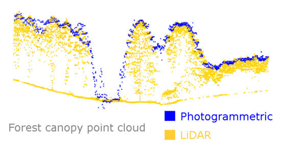
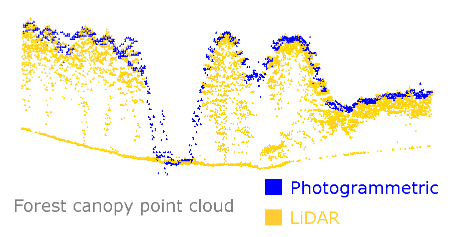
2.4.3. Dense Matching Strategy

Automated dense matching algorithms use image consistency/similarity measures (e.g., the normalized cross-correlation score) to establish a correspondence between homologous windows (matching windows) through image collection. The hierarchical matching approach of MICMAC starts with a first matching at a low resolution pyramid level. At each pyramid level, an intermediate canopy surface model is reconstructed and used in the subsequent level to provide the elevation approximations. The surface model computed from the higher level of the image pyramid is thus successively refined at each matching level, eventually resulting in a dense surface model. In order to refine the dense-matching result at a specific level of resolution, multiple matching processes may also occur successively at the same resolution. The matching strategy is defined as the sequence of coarse-to-fine hierarchical matching processes plus the value attributed to matching parameters at each matching level. The simplified tool, Malt, offers three predefined correlation strategies (GeomIm, urbanMNE and Ortho). Each correlation strategy is suited to a different type of scene geometry. In addition, the users have the opportunity to define their own matching strategy.

In the present study, the establishment of an optimal dense matching strategy for the deciduous canopy followed an iterative and trial-and-error procedure. It is often a complex process to set matching parameters to their appropriate value, as the meaning and exact effect of the matching parameters on the generated DSM are often not very clear [8]. Here, the key parameters determining the behavior of the matching algorithm that might impact forest canopy reconstruction were first identified. Secondly, the simplified tool, Malt, was utilized together with the predefined strategy, Ortho, for dense matching with the appropriate matching parameter values. After thorough inspection of the, Malt, results, it was concluded that this simplified tool did not offer the fine control required for forest photogrammetry. Thirdly, the complex tool, MICMAC, was utilized with a parametrization that was judged to be optimal for this purpose and for this type of imagery. Only this photo-DSM was subsequently compared with the LiDAR-CHM and forest inventory data. The outer canopy surface of irregular deciduous stands appears as a collection of rounded tree crowns of various sizes. Abrupt vertical changes occurring between trees (gaps) or between two stands are of primary importance to define the matching strategy [12]. In MICMAC, at least two parameters are related to the importance of vertical change: altimetric dilatation and the regularization factor. Dense matching occurs in terrain geometry, and the search space for matching homologous points in the image collection is thus defined within terrain geometry (coordinate system: Belgian Lambert 72). The search space is centered on the initial pixel position within the terrain geometry (X, Y, Z) (from the previous correlation level), which is bounded by a certain amount of dilatation in altimetry and planimetry. The level of altimetric dilatation needs to be high in order to fit any abrupt vertical changes. The regularization term expresses the a priori knowledge of the surface regularity [54]. Regularization represents the degree of smoothing and varies between 0 and 1: a high value means a high degree of smoothing. A low smoothing effect is assumed to be favorable to model the canopy structure [12]. Our preliminary investigations showed that a small matching window was suitable for a forest canopy scene. Moreover, a low correlation threshold was employed in order to force the matching over the complete scene.

The matching parameters, both used with, Malt and MICMAC, are summarized in Table 1. The optimal matching strategy (MICMAC) was found to be composed of six matching levels, proceeding from coarse resolution (1:32) to fine resolution (1:4). Regarding the expectation in terms of resolution and taking into account the fact that raw images were marred by blurring, it seemed more appropriate to use the final dense matching at a 1:4 resolution (GSD of 30 cm) than the original resolution (1:1).

Table 1. Parameters applied for multi-image, multi-resolution digital surface model (DSM) generation. The simplified tool, Malt, was not further used, since it did not offer the opportunity to finely adapt the altimetric dilatation.

Parameters	Value for Matching Strategy with Malt
Image pyramids	1:64–1:64–1:32–1:16–1:8–1:4–1:2–1:2
Regularization factor	0.005
Correlation window size	3 × 3
Minimum correlation coefficient	0
Minimal number of images visible in each ground point	3
Parameters	Value for Matching Strategy with MICMAC
Image pyramids	1:32–1:16-1:16–1:16–1:8–1:4
Altimetric dilatation	15–15–8–8–8–8
Regularization factor	0.05–0.05–0.001–0.001–0.001–0.003
Correlation window size	3 × 3
Minimum correlation coefficient	0
Minimal number of image visible in each ground point	3

Table 1. Parameters applied for multi-image, multi-resolution digital surface model (DSM) generation. The simplified tool, Malt, was not further used, since it did not offer the opportunity to finely adapt the altimetric dilatation.

Parameters	Value for Matching Strategy with Malt
Image pyramids	1:64–1:64–1:32–1:16–1:8–1:4–1:2–1:2
Regularization factor	0.005
Correlation window size	3 × 3
Minimum correlation coefficient	0
Minimal number of images visible in each ground point	3
Parameters	Value for Matching Strategy with MICMAC
Image pyramids	1:32–1:16-1:16–1:16–1:8–1:4
Altimetric dilatation	15–15–8–8–8–8
Regularization factor	0.05–0.05–0.001–0.001–0.001–0.003
Correlation window size	3 × 3
Minimum correlation coefficient	0
Minimal number of image visible in each ground point	3

2.5. Investigation of Photo-CHM Quality

The accuracy of photogrammetric DSMs relies on many interacting factors (e.g., the complexity of the visible surface, camera type, photographic quality, sun-object-sensor geometry, etc. [58]). The forest canopy surface is very complex (high variation in micro-relief, reflectance anisotropy), and the matching accuracy for such a surface may be marred by: (1) little or no texture (pattern created by adjacent leaves and crowns); (2) object discontinuities; (3) repetitive objects; (4) moving objects (such as leaves, tree apex and shadows); (5) occlusions; (6) multi-layered or transparent objects; and (7) radiometric artifacts [8,30,59]. Besides, UAS imagery is characterized by low-oblique vantage: the sun-object-sensor geometry is highly variable between different images. The sun-canopy-sensor geometry impacts the brightness pattern of a crown, e.g., the location of the hot spot (i.e., the spot in direct alignment with the sun and camera, which is brighter than its surroundings [43]). The accuracy of DSMs reconstructed by image matching techniques has been investigated by Kraus et al. [60] using an error propagation approach. Hybrid photo-LiDAR CHMs (referred to as photo-CHMs) are also sensitive to the co-registration procedure. Assessment of surface matching for co-registration was investigated and well detailed by Lin et al. [61]. In this research, the quality of the photo-CHM was investigated using different approaches. The photo-CHM was not sufficiently accurate to be the subject of a rigorous validation, due to the time discrepancy between photo and LiDAR acquisition. Instead, investigations were carried out in order to compare the use of photo-CHM with LiDAR-CHM in the field of forest sciences. First of all, the photo-CHM was cropped by 100 m around its edges in order to avoid a gross variation in image overlap. Overall accuracy was then estimated by a cloud to cloud comparison using CloudCompare. Cloud to cloud distance was computed using a “least squares plane” local surface model for the master point cloud. Moreover, subtraction of the LiDAR-CHM from the photo-CHM grids brought insight into their altimetric differences. As the LiDAR survey has been carried out 1 year before the UAS flight, this comparison highlighted the trees that had been harvested during the interval between the two surveys.

Tests were also carried out to determine how satisfactorily forest variables might be derived from photo-CHM. Single tree and structural forest attributes are commonly extracted from CHMs by means of a regression model predicting forest variables (exploratory variables) with metrics (explanatory variables) [12,13]. These metrics are used to synthesize the CHM in a particular area (stand, plot or window, crown), such as the mean height, the standard height deviation or the height at a certain percentile. Three area-based methods were tested, corresponding to different object levels:

• Window level: metrics using 20 m × 20 m windows were computed for both CHMs and correlation coefficients between photo-CHM and LiDAR-CHM metrics were calculated. This comparison technique was first introduced by St-Onge et al. [32]. The technique gives an overall idea of the photo-CHM and LiDAR-CHM correlation stand metrics, but has only a poor ecological meaning. Metrics were correlated only for forested windows: crop fields and meadow areas were therefore discarded. Forested areas were identified by means of the forest stand localization map and a mean height threshold of 3 m.
• Stand level: stand models were constructed based on inventory data (plot inventory) for predicting dominant height. The model residual (residual mean square error) and the model fit coefficient ($r^2$) served as indicators of CHMs quality. For each CHM, two regression models were adjusted, the first with one single explanatory variable and the second with two explanatory variables. The selection of these variables was performed with the best subset regression analysis.
• Tree level: the model for individual tree heights was established. Tree crowns were delineated by hand by a photo interpreter, and metrics were computed on this crown area. The best model, using only one metric, was selected using the best subset regression procedure. Its performance was presented in terms of RMSE (residual mean square error) and model fit coefficient ($r^2$).

Before the extraction of height metrics, the height values below 2 m were preliminarily discarded from the CHMs in order to mitigate the effect of bare soil, grass and small shrubs, which might impact the forest canopy height [12,33]. The metrics extracted for windows, stand and tree level were: the mean, max ($p100$), min ($p0$), the first, second and third quartile ($p25$, $p50$ and $p75$) and the 90th, 92.5th, 95th, 97.5th and 99th percentiles ($p90$, $p925$, $p95$, $p975$ and $p99$). In addition, the standard deviation was extracted for dominant height regression analysis ($sd$). Linear regression analyses (tree-wise and stand-wise models) were similarly carried out on LiDAR-CHM metrics in order to compare the model accuracy of photo-CHM and LiDAR-CHM. All the regression analyses were performed using the [R] statistical software [62].

3. Results

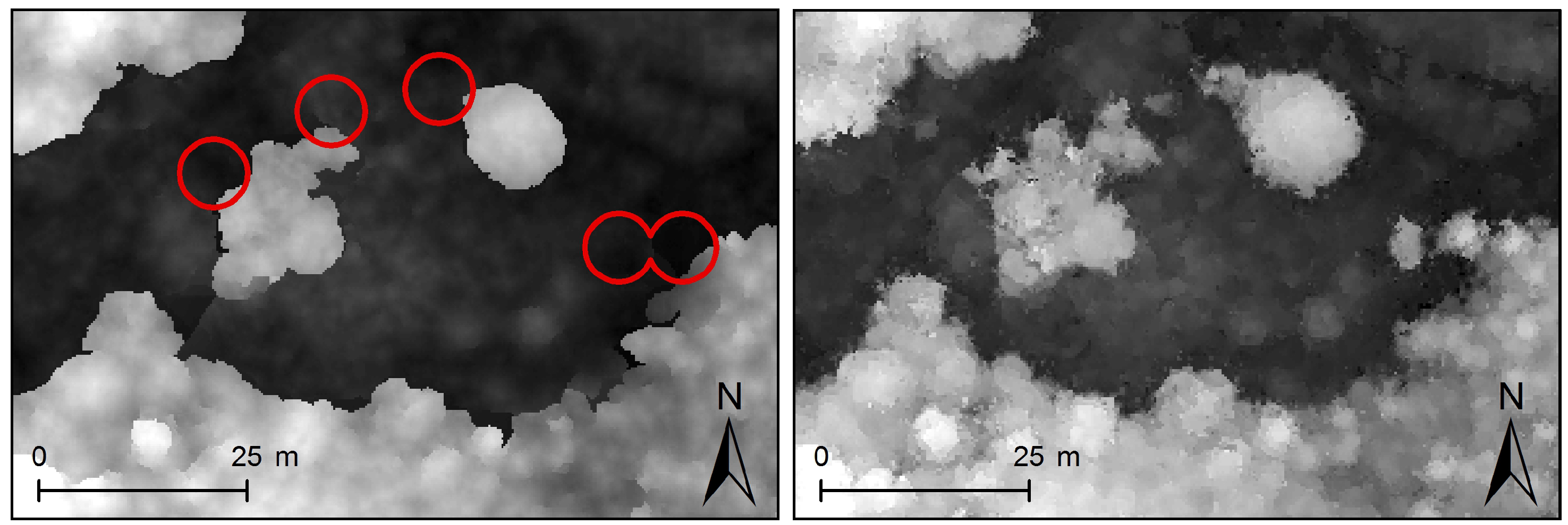
3.1. Photo-DSM Generation

Absolute orientation was successful for 439 out of 441 images. Two images on the image block border were discarded, because their orientation appeared to be wrong. A total of 91 kilo tie point positions were adjusted, with a mean residual of 0.87 pixels (reprojection error). Figure 2 presents one of the individual aerial images and the results of the automatic aerotriangulation.

Figure 2. Elements of the orientation of individual aerial images were computed by automatic aerotriangulation. (Left) One of the 439 images; (Right) the aerotriangulated model. Camera poses are displayed with green dots.

Figure 2. Elements of the orientation of individual aerial images were computed by automatic aerotriangulation. (Left) One of the 439 images; (Right) the aerotriangulated model. Camera poses are displayed with green dots.

Registration of the approximated georeferenced model with the LiDAR-DSM was seen as satisfactory, as the mean distance between the two point clouds was 0.48 m with a standard deviation of 0.44 m.

A visual inspection and comparison of both surface models resulting from the two matching strategies (implemented in the simple and the complex tools for dense-matching, Malt and MICMAC) suggested that the overall quality of the reconstruction is good. The matching strategies were optimized for deciduous canopy reconstruction; it was thus not surprising that conifers were not adequately reconstructed. Indeed, coniferous crowns are often partially reconstructed. In addition, an in-depth visual comparison highlighted the fact that some isolated deciduous trees were absent from the canopy surface model that was generated with Malt, although they were well represented in the aerial images. Figure 3 illustrates these omissions, which were resolved by raising the altimetric dilatation and decreasing the degree of regularization. Striking differences found between the two surface models were mainly due to the difference in the degree of smoothing, also controlled by the regularization term.

Figure 3. Comparison of two matching strategies: Malt (Left) and MICMAC (Right). Red circles highlight the positions of trees that have not been reconstructed with Malt. The optimal photo-DSM used, further, is the DSM produced with MICMAC.

Figure 3. Comparison of two matching strategies: Malt (Left) and MICMAC (Right). Red circles highlight the positions of trees that have not been reconstructed with Malt. The optimal photo-DSM used, further, is the DSM produced with MICMAC.

Figure 4 shows a close-up of the photo-DSM on a shaded view and the corresponding correlation map. Mature deciduous tree crowns are easily identifiable on the upper forest stand, but, by contrast, tree crowns in the young plantation (bottom of the figure) are not easily visually distinguished.

Figure 4. Close-up of the canopy surface model. (Left) The canopy surface model; (Center) map of the normalized cross-correlation score, expressing the similarity of the images (the normalized cross-correlation score ranges from zero (dark area, low similarity) to one (white area, high similarity)); (Right) false color ortho-photo mosaic.

Figure 4. Close-up of the canopy surface model. (Left) The canopy surface model; (Center) map of the normalized cross-correlation score, expressing the similarity of the images (the normalized cross-correlation score ranges from zero (dark area, low similarity) to one (white area, high similarity)); (Right) false color ortho-photo mosaic.

3.2. Investigation of Photo-CHM Quality

3.2.1. Overall Comparison of Photo-CHM and LiDAR-CHM

As the time interval between the LiDAR and the UAS survey was one year, the LiDAR-CHM was not a perfectly sound reference for the photo-CHM. In addition to differences due strictly to the two acquisition techniques, there was an effect of vegetation growth and of harvested trees. The author of Gruen [63] has highlighted that the key problem with carrying out an accuracy test for photo-DSMs is the capacity to dispose of sufficiently good reference data. However, as the comparison here was performed on the complete CHM, average distance was not sensitive to local and extreme differences (e.g., harvested trees).

Cloud to cloud distance showed that planimetric standard deviation was about 0.46 m. Altimetric distance revealed the presence of a negative bias of 2.4 cm, attributable to the unreconstructed small gaps between tree crowns. Standard deviation in the Z distance was 0.48 cm. A visual comparison of a transect for both LiDAR and photogrammetric point clouds is illustrated in Figure 5.

Figure 5. Comparison between photogrammetric and LiDAR point clouds. LiDAR pulses penetrate the forest canopy and better account for small gaps and peaks, than the photogrammetric point cloud.

Figure 5. Comparison between photogrammetric and LiDAR point clouds. LiDAR pulses penetrate the forest canopy and better account for small gaps and peaks, than the photogrammetric point cloud.

Figure 6. Evaluation of the differences between LiDAR and photo canopy height models: enlargement of a small part of the Felenne forest for visual comparison (units are in meters). (Top Left) photo-canopy height model (CHM); (Top Right) LiDAR-CHM; (Bottom Left) difference in elevation between photo-CHM and LiDAR-CHM; (Bottom Right) false color ortho-photo mosaic.

Figure 6. Evaluation of the differences between LiDAR and photo canopy height models: enlargement of a small part of the Felenne forest for visual comparison (units are in meters). (Top Left) photo-canopy height model (CHM); (Top Right) LiDAR-CHM; (Bottom Left) difference in elevation between photo-CHM and LiDAR-CHM; (Bottom Right) false color ortho-photo mosaic.

Subtraction of the LiDAR-CHM from the photo-CHM is illustrated in Figure 6. Small gaps and tree tops are better represented in the LiDAR-CHM. Crowns are generally wider and less defined in photo-CHMs, as has already been observed in previous comparisons of photo-DSMs with LiDAR-DSMs [32]. The visual quality of the photo-CHM varies among stand species and density. Particularly, coniferous stands with low tree density (with numerous and abrupt fine-scale peaks and gaps in the outer canopy) seem to suffer more from the smoothing effect induced by the dense-matching. What is interesting to note is that serious underestimations (black areas) of the canopy height occurred exclusively in specific cases: where there were object discontinuities (stand edge and isolated conifers presenting abrupt vertical changes) and where trees had been harvested during the interval between the LiDAR and UAS surveys (e.g., north-south corridor of trees on the left-hand side, surrounded by a red line, and isolated trees near the scale bar). Overestimations (white areas) of photo-CHM occurred as a result of occlusions, shadows and smoothing. The complete photo-CHM and LiDAR-CHM maps are provided in the supplementary material.

Table 2. Correlation between photo-CHM and LiDAR-CHM window metrics. Bold figures represent the highest correlation scores.

		Photo-CHM Metrics
		Mean	$\mathit{p}\mathbf{0}$	$\mathit{p}\mathbf{25}$	$\mathit{p}\mathbf{50}$	$\mathit{p}\mathbf{75}$	$\mathit{p}\mathbf{90}$	$\mathit{p}\mathbf{925}$	$\mathit{p}\mathbf{95}$	$\mathit{p}\mathbf{975}$	$\mathit{p}\mathbf{99}$	$\mathit{p}\mathbf{100}$
LiDAR-CHM Metrics	Mean	0.96	0.67	0.93	0.95	0.91	0.86	0.85	0.84	0.82	0.80	0.74
	p0	0.17	0.27	0.20	0.16	0.12	0.10	0.10	0.10	0.09	0.09	0.07
	p25	0.87	0.77	0.92	0.84	0.76	0.69	0.67	0.66	0.64	0.62	0.56
	p50	0.96	0.62	0.93	0.96	0.90	0.84	0.82	0.81	0.78	0.76	0.72
	p75	0.93	0.49	0.83	0.93	0.95	0.92	0.91	0.89	0.87	0.85	0.81
	p90	0.88	0.42	0.76	0.87	0.93	0.94	0.94	0.93	0.92	0.90	0.86
	p925	0.87	0.41	0.75	0.86	0.92	0.94	0.93	0.93	0.92	0.90	0.86
	p95	0.86	0.39	0.73	0.84	0.91	0.93	0.93	0.93	0.92	0.91	0.87
	p975	0.85	0.38	0.72	0.82	0.89	0.92	0.92	0.92	0.92	0.91	0.88
	p99	0.83	0.37	0.71	0.81	0.88	0.91	0.91	0.92	0.92	0.91	0.88
	p100	0.80	0.35	0.68	0.78	0.85	0.88	0.88	0.89	0.89	0.89	0.86

Table 2. Correlation between photo-CHM and LiDAR-CHM window metrics. Bold figures represent the highest correlation scores.

		Photo-CHM Metrics
		Mean	$\mathit{p}\mathbf{0}$	$\mathit{p}\mathbf{25}$	$\mathit{p}\mathbf{50}$	$\mathit{p}\mathbf{75}$	$\mathit{p}\mathbf{90}$	$\mathit{p}\mathbf{925}$	$\mathit{p}\mathbf{95}$	$\mathit{p}\mathbf{975}$	$\mathit{p}\mathbf{99}$	$\mathit{p}\mathbf{100}$
LiDAR-CHM Metrics	Mean	0.96	0.67	0.93	0.95	0.91	0.86	0.85	0.84	0.82	0.80	0.74
	p0	0.17	0.27	0.20	0.16	0.12	0.10	0.10	0.10	0.09	0.09	0.07
	p25	0.87	0.77	0.92	0.84	0.76	0.69	0.67	0.66	0.64	0.62	0.56
	p50	0.96	0.62	0.93	0.96	0.90	0.84	0.82	0.81	0.78	0.76	0.72
	p75	0.93	0.49	0.83	0.93	0.95	0.92	0.91	0.89	0.87	0.85	0.81
	p90	0.88	0.42	0.76	0.87	0.93	0.94	0.94	0.93	0.92	0.90	0.86
	p925	0.87	0.41	0.75	0.86	0.92	0.94	0.93	0.93	0.92	0.90	0.86
	p95	0.86	0.39	0.73	0.84	0.91	0.93	0.93	0.93	0.92	0.91	0.87
	p975	0.85	0.38	0.72	0.82	0.89	0.92	0.92	0.92	0.92	0.91	0.88
	p99	0.83	0.37	0.71	0.81	0.88	0.91	0.91	0.92	0.92	0.91	0.88
	p100	0.80	0.35	0.68	0.78	0.85	0.88	0.88	0.89	0.89	0.89	0.86

3.2.2. Window Level

The correlation scores of the windows-based LiDAR-CHM/photo-CHM metrics are presented in Table 2. The highest correlation score reached 0.96 for the mean height and the 50th percentiles. The lower correlation scores for the low percentiles supports the previous finding highlighted by visual comparison: fine-scale gaps could not be correctly reconstructed by image matching. This is due to the problem of “dead-ground” [42]: leaves and branches in the foreground of an image obscure the ground, resulting in significant omissions. It is a well-know limitation of aerial images that dense canopy cover occludes and casts shadows over understory features [33]. These omissions were only partly taken into account in this comparison, as objects close to the ground (vegetation height below 2 m) were discarded from both CHMs. In addition, this table of correlation scores demonstrates that photo-CHM is equivalent to a smoothed LiDAR-CHM. The table shows that low photo-CHM percentiles tended to be well correlated with higher LiDAR-CHM percentiles and that, by contrast, high photo-CHM percentiles tended to be well correlated with lower LiDAR-CHM percentiles. Although fine-scale peaks and gaps in the outer canopy were not perfectly modeled by image matching, the high correlation score may reflect the fact that this type of canopy surface smoothing remains quite soft in comparison with high altitude airborne imagery in which omissions are even more omnipresent. As a comparison, the correlation of metrics reached a maximum of 0.95 in the study of St-Onge et al. [32] (using airborne images), but without discarding height values under 2 m, thus keeping the height variability higher. In the present study, performing the same analysis on CHM without discarding values under 2 m raised the correlation coefficient to 0.98 between the 99th percentile in the photo-CHM and the 99th percentile in the LiDAR-CHM.

3.2.3. Stand Level

A summary of field inventory measures shows the high variability between stands in terms of density (number of trees per ha, basal area and volume per ha), on the one hand, and in terms of maturity (dominant height), on the other hand. Dominant heights range from 9.6 to 27.3 m, with an average of 19.7 m (Table 3). Individual heights of dominant trees varied considerably within the same stand, with a mean standard deviation of 1.6 m across the set of field plots. This shows the degree of structure irregularity in these deciduous stands.

Table 3. Characteristics of deciduous stands. Statistics were obtained from the 36 measured field plots (mean, minimum, maximum and standard deviation values).

	Mean	Minimum	Maximum	Standard Deviation
Plot radius (m)	13.2	7.4	18	3.8
Number of trees (n/ha)	537.3	69	1,395	336.7
Basal area (m2/ha)	21.8	3.6	46.2	9.8
Total volume (m3/ha)	277	25.1	570.1	147.6
Dominant height (m)	19.7	9.6	27.3	3.9

Table 3. Characteristics of deciduous stands. Statistics were obtained from the 36 measured field plots (mean, minimum, maximum and standard deviation values).

	Mean	Minimum	Maximum	Standard Deviation
Plot radius (m)	13.2	7.4	18	3.8
Number of trees (n/ha)	537.3	69	1,395	336.7
Basal area (m2/ha)	21.8	3.6	46.2	9.8
Total volume (m3/ha)	277	25.1	570.1	147.6
Dominant height (m)	19.7	9.6	27.3	3.9

The selected dominant height models are presented in Table 4. Models based on LiDAR-CHM metrics performed better than models based on photo-CHM, but the difference appears to be small. Indeed, the model fit of 0.86 for LiDAR-CHM drops down to 0.82 for photo-CHM, and the RMSE increases from 7.4% to 8.4% (for Model 2). Moreover, paired t-tests showed that only the residuals of Model 1 and Model 3 are significantly different, but the performance of the photo-CHM model with two explanatory variables is similar to LiDAR-based models in terms of residuals. Height variability has a greater significance under the 99th percentile metric ($p99$) in Model 1 rather than under the maximum height ($p100$). This highlights the occasional presence of blunders (high values). This is due to the low degree of regularization set in the dense-matching strategy. The regression models with two metrics showed that the combination of mean height and standard deviation describes more precisely the distribution of vegetation height and explains better the tree height than solely the 99th height percentile on its own, although the difference in RMSE is low.

Table 4. Comparison of dominant height ($Hdom$) models for deciduous irregular stands (n = 36) based on photo-CHM and LiDAR-CHM metrics. Model performance is described in terms of adjusted $r^2$, root-mean-square error (RMSE) (m) and relative RMSE (%). ID stands for model identification number.

CHM	ID	Regression Model Form	Explanatory	$r^2$ Adjusted	RMSE (m)	RMSE (%)
			Variable(s)
Photo-CHM	1	$Hdom=\alpha +\beta \times p99$	$p99$	0.82	1.68	8.5
Photo-CHM	2	$Hdom=\alpha +\beta \times mean+\gamma \times sd$	$mean$, $sd$	0.82	1.65	8.4
LiDAR-CHM	3	$Hdom=\alpha +\beta \times p100$	$p100$	0.86	1.45	7.4
LiDAR-CHM	4	$Hdom=\alpha +\beta \times mean+\gamma \times sd$	$mean$, $sd$	0.86	1.45	7.4

Table 4. Comparison of dominant height ($Hdom$) models for deciduous irregular stands (n = 36) based on photo-CHM and LiDAR-CHM metrics. Model performance is described in terms of adjusted $r^2$, root-mean-square error (RMSE) (m) and relative RMSE (%). ID stands for model identification number.

CHM	ID	Regression Model Form	Explanatory	$r^2$ Adjusted	RMSE (m)	RMSE (%)
			Variable(s)
Photo-CHM	1	$Hdom=\alpha +\beta \times p99$	$p99$	0.82	1.68	8.5
Photo-CHM	2	$Hdom=\alpha +\beta \times mean+\gamma \times sd$	$mean$, $sd$	0.82	1.65	8.4
LiDAR-CHM	3	$Hdom=\alpha +\beta \times p100$	$p100$	0.86	1.45	7.4
LiDAR-CHM	4	$Hdom=\alpha +\beta \times mean+\gamma \times sd$	$mean$, $sd$	0.86	1.45	7.4

Dominant tree height was measured from the photo-CHM with a standard error of 1.65 m. Although these RMSEs are slightly higher than in the results from comparable research, we interpret our results as being quite favorable within the context of irregular stands. As a comparison, Dandois and Ellis [33] predicted dominant height with a single explanatory variable extracted from a UAS photo-CHM with a model fit of 0.84 and an RMSE of 3.2 m.

3.2.4. Tree Level

In total, 86 trees were measured and their crowns delineated on both photo-CHM and LiDAR-CHM. Tree heights range from 10.5 to 29.4 m, with an average of 22.3 m. The regression models are summarized in Table 5. For both photo-CHM and LiDAR-CHM, root-mean-squared residuals reduced to 5%, supporting the assumption that individual tree height can be measured with an acceptable level of accuracy using a CHM. As a comparison, St-Onge et al. [64] photo-interpreted the tree height of 202 white cedars (mean height of 8 m) (Thuja occidentalis) in classic aerial stereo pairs (GSD of 11 cm), registered with LiDAR-DTM. This yielded an average deviation of 1.94 m at the 90th percentile. Studies using a lightweight LiDAR UAS platform have demonstrated that it is possible to measure individual tree heights with a standard deviation of 30 cm [36] and even 15 cm when a very high pulse density is used [35].

Table 5. Comparison of individual tree height models (n = 86) based on photo-CHM and LiDAR-CHM metrics. Model performance is described in terms of adjusted $r^2$, RMSE (m), relative RMSE (%) and average deviation at the 90th percentile (${\left|ϵ\right|}_{90}$).

CHM	Explanatory Variable	$r^2$ Adjusted	RMSE (m)	RMSE (%)	${\left|ϵ\right|}_{90}$
Photo-CHM	$p975$	0.91	1.04	4.7	1.58
LiDAR-CHM	$p975$	0.94	0.83	3.7	1.23

Table 5. Comparison of individual tree height models (n = 86) based on photo-CHM and LiDAR-CHM metrics. Model performance is described in terms of adjusted $r^2$, RMSE (m), relative RMSE (%) and average deviation at the 90th percentile (${\left|ϵ\right|}_{90}$).

CHM	Explanatory Variable	$r^2$ Adjusted	RMSE (m)	RMSE (%)	${\left|ϵ\right|}_{90}$
Photo-CHM	$p975$	0.91	1.04	4.7	1.58
LiDAR-CHM	$p975$	0.94	0.83	3.7	1.23

4. Conclusions and Perspectives

This study has confirmed that UAS imagery, combined with a LiDAR-DTM that is available beforehand, is promising for forest height measurement. The open source suite, MICMAC was shown to freely provide both simple and complex photogrammetric tools. These tools suit very well the fine-tuning requirements to overcome major issues experienced when undertaking photogrammetry in forest areas. Adaptation of matching parameters, such as altimetric dilatation, the regularization term, correlation windows and the correlation threshold, was shown to be successful in the production of a photogrammetric canopy surface model visually coherent with the canopy structure. Surface matching was shown to perform a co-registration procedure of photo-DSM with LiDAR-DSM with a cloud to cloud altimetric distance of 0.48 m (standard deviation). This result is in accordance with accuracy requirements.

Comparison of photo-CHM with LiDAR-CHM, on the one hand, and field inventory measurements (individual tree height measurements and stand-wise inventory), on the other hand, brought insight regarding photo-CHM quality. Photo-CHM and LiDAR-CHM window-based metrics were found to be very well correlated (up to 0.96 (r)). Discarding low vegetation height values, in order to limit the influence of ground, rock and shrubs, considerably impacted these correlation measurements. Indeed, computed metrics taking into account low vegetation height were shown to be even more correlated (r up to 0.98). Regression models at stand level (dominant height) and at tree level (individual height) were shown to perform well. It was thus possible to predict dominant height with an RMSE of 8.4% (1.65 m, $r^2$ of 0.82) and individual height with an RMSE of 4.7% (1.04 m, $r^2$ of 0.91) based on photo-CHM. LiDAR-CHM models performed slightly better than photo-CHM models, although differences in terms of model fit and root mean square residuals were no more than a few percent. These regression models only give an overview of the possibility of extracting dendrometric data from high resolution photo-CHM. Indeed, a thorough validation of the photogrammetric forest canopy model would require further specific research. As previously stated, a key problem for the validation of photogrammetric results lies in the difficulty of obtaining sufficiently accurate and contemporary reference data.

The results gained in this study through empirical tests of the quality of photo-CHM need to be interpreted with caution, as both reference datasets (LiDAR-CHM and field inventory data) showed their limitations. The time discrepancy between the LiDAR and the UAS surveys certainly hampered the comparison of the photo-CHM with the LiDAR-CHM. Indeed, the harvesting of trees during the interval between the two surveys explains the majority of the differences found between the photo-CHM and LiDAR-CHM. Furthermore, field data, in particular. deciduous tree heights, were marred by a relatively low level of accuracy. In addition, the forest inventory sampling scheme was optimized for delivering indicators on stand density, structure and maturity, but was not ideally suited to photo-CHM validation. We recommend the use of a fixed-size field plot for the validation of photo-CHM. We also recommend, on this plot surface, the measurement of trees for which the crown is present. even if their stems fall outside the plot area. Moreover, measuring the dominant height of irregular deciduous stands is of limited interest and is much more difficult, as dominant height is a less well-defined concept in uneven-aged stands than in regular stands. Eventually, either the generation or the validation of photo-CHM needs to be adapted to a specific structure: we observed in the present study that our optimal matching strategy was better suited to deciduous stands than to conifer stands. Photo-DSM also showed different degrees of success according to the density of the stand: stands with continuous canopy cover were much more accurately reconstructed than stands presenting local gaps between tree crowns. Finally, the abrupt vertical changes were difficult to model accurately, even with UAS imagery. Different acquisition strategies can also strongly interfere in the dense matching process, e.g., the images overlap or the flight altitude [33]. Further research needs to be undertaken in order to define an appropriate template for UAS acquisition in forested areas.

The original processing workflow developed in this study has shown that photogrammetry can be used for forest mapping and forest planning, although there is still a lot of room for future improvement. As a comparison of UAS data with LiDAR data was the central focus in this paper, we would emphasize our view of photogrammetry as being more a complement rather than a surrogate for LiDAR. The use of photogrammetry within the field of precision forestry allows for the monitoring of the forest structural evolutions through multi-date image acquisition on a local scale. High resolution ortho-photo mosaics are likely to be used for forest stand delineation and mapping, and CHM-based forest regression models can be advantageously adjusted in order to carry out multi-source inventories. Finely-tuned indicators of forest structure also need to be determined in addition to classic density forest indicators, such as volume, basal area and the number of trees per hectare. Indeed, dominant height and other classic measures of stand height cannot account for irregular stand characteristics. As a complement to our approach, regression models predicting forest variables also need to take advantage of spectral information [27]. Obviously, the generation of ortho-photo mosaics is a prerequisite for the use of spectral information. The ortho-rectification process also needs to be adapted for forest scenes and UAS imagery (e.g., radiometric equalization would be required in order to account for illumination variation occurring during UAS acquisition). In addition to quantitative regression models, forest species composition could also be determined (e.g., by means of supervised classification) based on the spectral information from time-series of ortho-photo mosaics.

The photogrammetric toolbox, MICMAC, remains under constant development. We can expect future improvements to simplify the use of the MICMAC tools. We can also anticipate an increase in the amount of related documentation, such as the present case study, with the growth of the community of users. Moreover, we can expect several improvements in the future regarding UAS photogrammetry as applied to forestry. Matching strategies need to take into account the forest type (mainly composition and structure). Visual inspection of the photo-DSM has highlighted differences in terms of quality between deciduous stands with a closed canopy and coniferous stands with gaps between tree crowns. At least two matching strategies need to be established and performed, one for deciduous stands and another for coniferous stands. Previous information on the scene also needs to be integrated into the workflow [63]. For example, LiDAR-DSM could be used as an initial value for hierarchical matching, thus reducing the risk of false matching, as well as computational time. Significant savings of computational time could be achieved in the construction of photo-CHM time series: a previously obtained photo-DSM could serve as the initial value for upcoming photo-DSM generation.

References

1. Watts, A.C.; Ambrosia, V.G.; Hinkley, E.A. Unmanned aircraft systems in remote sensing and scientific research: Classification and considerations of use. Remote Sens. 2012, 4, 1671–1692. [Google Scholar] [CrossRef]
2. Anderson, K.; Gaston, K.J. Lightweight unmanned aerial vehicles will revolutionize spatial ecology. Front. Ecol. Environ. 2013, 11. [Google Scholar] [CrossRef]
3. Turner, D.; Lucieer, A.; Watson, C. An automated technique for generating georectified mosaics from ultra-high resolution unmanned aerial vehicle (UAV) imagery, based on structure from motion (SfM) point clouds. Remote Sens. 2012, 4, 1392–1410. [Google Scholar] [CrossRef]
4. Koh, L.P.; Wich, S.A. Dawn of drone ecology: Low-cost autonomous aerial vehicles for conservation. Trop. Conserv. Sci. 2012, 5, 121–132. [Google Scholar]
5. Haala, N. Comeback of digital image matching. Photogram. Week 2009, 9, 289–301. [Google Scholar]
6. Pierrot-Deseilligny, M.; Clery, I. Évolutions récentes en photogrammétrie et modélisation 3d par photo des milieux naturels. Collect. EDYTEM 2011, 12, 51–64. [Google Scholar]
7. Snavely, N.; Seitz, S.M.; Szeliski, R. Modeling the world from internet photo collections. Int. J. Comput. Vis. 2008, 80, 189–210. [Google Scholar] [CrossRef]
8. Baltsavias, E.; Gruen, A.; Eisenbeiss, H.; Zhang, L.; Waser, L.T. High-quality image matching and automated generation of 3D tree models. Int. J. Remote Sens. 2008, 29, 1243–1259. [Google Scholar] [CrossRef]
9. Dandois, J.P.; Ellis, E.C. Remote sensing of vegetation structure using computer vision. Remote Sens. 2010, 2, 1157–1176. [Google Scholar] [CrossRef]
10. Corona, P.; Fattorini, L. Area-based lidar-assisted estimation of forest standing volume. Can. J. For. Res. 2008, 38, 2911–2916. [Google Scholar] [CrossRef] [Green Version]
11. Steinmann, K.; Mandallaz, D.; Ginzler, C.; Lanz, A. Small area estimations of proportion of forest and timber volume combining lidar data and stereo aerial images with terrestrial data. Scand. J. For. Res. 2013, 28, 373–385. [Google Scholar] [CrossRef]
12. Næsset, E. Predicting forest stand characteristics with airborne scanning laser using a practical two-stage procedure and field data. Remote Sens. Environ. 2002, 80, 88–99. [Google Scholar] [CrossRef]
13. Næsset, E.; Gobakken, T.; Holmgren, J.; Hyyppä, H.; Hyyppä, J.; Maltamo, M.; Nilsson, M.; Olsson, H.; Persson, A.; Söderman, U. Laser scanning of forest resources: The Nordic experience. Scand. J. For. Res. 2004, 19, 482–499. [Google Scholar] [CrossRef]
14. Wehr, A.; Lohr, U. Airborne laser scanning—An introduction and overview. J. Photogram. Remote Sens. 1999, 54, 68–82. [Google Scholar] [CrossRef]
15. Zimble, D.A.; Evans, D.L.; Carlson, G.C.; Parker, R.C.; Grado, S.C.; Gerard, P.D. Characterizing vertical forest structure using small-footprint airborne LiDAR. Remote Sens. Environ. 2003, 87, 171–182. [Google Scholar] [CrossRef]
16. Maltamo, M.; Eerikäinen, K.; Packalén, P.; Hyyppä, H. Estimation of stem volume using laser scanning-based canopy height metrics. Forestry 2006, 79, 217–229. [Google Scholar] [CrossRef]
17. Miura, N.; Jones, S.D. Characterizing forest ecological structure using pulse types and heights of airborne laser scanning. Remote Sens. Environ. 2010, 114, 1069–1076. [Google Scholar] [CrossRef]
18. Jaskierniak, D.; Lane, P.N.J.; Robinson, A.; Lucieer, A. Extracting LiDAR indices to characterise multilayered forest structure using mixture distribution functions. Remote Sens. Environ. 2011, 115, 573–585. [Google Scholar] [CrossRef]
19. Zhao, K.G.; Popescu, S.; Meng, X.L.; Pang, Y.; Agca, M. Characterizing forest canopy structure with lidar composite metrics and machine learning. Remote Sens. Environ. 2011, 115, 1978–1996. [Google Scholar] [CrossRef]
20. Lindberg, E.; Hollaus, M. Comparison of methods for estimation of stem volume, stem number and basal area from airborne laser scanning data in a hemi-boreal forest. Remote Sens. 2012, 4, 1004–1023. [Google Scholar] [CrossRef]
21. Baltsavias, E.P. A comparison between photogrammetry and laser scanning. ISPRS J. Photogram. Remote Sens. 1999, 54, 83–94. [Google Scholar] [CrossRef]
22. Lim, K.; Treitz, P.; Wulder, M.; St-Onge, B.; Flood, M. LiDAR remote sensing of forest structure. Progr. Phys. Geogr. 2003, 27, 88–106. [Google Scholar] [CrossRef]
23. Hyyppä, J.; Hyyppä, H.; Leckie, D.; Gougeon, F.; Yu, X.; Maltamo, M. Review of methods of small-footprint airborne laser scanning for extracting forest inventory data in boreal forests. Int. J. Remote Sens. 2008, 29, 1339–1366. [Google Scholar] [CrossRef]
24. Véga, C.; St-Onge, B. Mapping site index and age by linking a time series of canopy height models with growth curves. For. Ecol. Manag. 2009, 257, 951–959. [Google Scholar] [CrossRef]
25. Véga, C.; St-Onge, B. Height growth reconstruction of a boreal forest canopy over a period of 58 years using a combination of photogrammetric and lidar models. Remote Sens. Environ. 2008, 112, 1784–1794. [Google Scholar] [CrossRef] [Green Version]
26. Huang, H.; Gong, P.; Cheng, X.; Clinton, N.; Li, Z. Improving measurement of forest structural parameters by co-registering of high resolution aerial imagery and low density LiDAR data. Sensors 2009, 9, 1541–1558. [Google Scholar] [CrossRef] [PubMed]
27. Bohlin, J.; Wallerman, J.; Fransson, J.E.S. Forest variable estimation using photogrammetric matching of digital aerial images in combination with a high-resolution DEM. Scand. J. For. Res. 2012, 27, 692–699. [Google Scholar] [CrossRef]
28. Mora, B.; Wulder, M.A.; Hobart, G.W.; White, J.C.; Bater, C.W.; Gougeon, F.A.; Varhola, A.; Coops, N.C. Forest inventory stand height estimates from very high spatial resolution satellite imagery calibrated with lidar plots. Int. J. Remote Sens. 2013, 34, 4406–4424. [Google Scholar] [CrossRef]
29. Nurminen, K.; Karjalainen, M.; Yu, X.; Hyyppä, J.; Honkavaara, E. Performance of dense digital surface models based on image matching in the estimation of plot-level forest variables. ISPRS J. Photogram. Remote Sens. 2013, 83, 104–115. [Google Scholar] [CrossRef]
30. White, J.; Wulder, M.; Vastaranta, M.; Coops, N.; Pitt, D.; Woods, M. The utility of image-based point clouds for forest inventory: A comparison with airborne laser scanning. Forests 2013, 4, 518–536. [Google Scholar] [CrossRef]
31. Eisenbeiss, H. UAV Photogrammetry. Ph.D. Thesis, ETH, Zurich, Switzerland, 2009. [Google Scholar]
32. St-Onge, B.; Vega, C.; Fournier, R.A.; Hu, Y. Mapping canopy height using a combination of digital stereo-photogrammetry and lidar. Int. J. Remote Sens. 2008, 29, 3343–3364. [Google Scholar] [CrossRef]
33. Dandois, J.P.; Ellis, E.C. High spatial resolution three-dimensional mapping of vegetation spectral dynamics using computer vision. Remote Sens. Environ. 2013, 136, 259–276. [Google Scholar] [CrossRef]
34. Tao, W.; Lei, Y.; Mooney, P. Dense Point Cloud Extraction from UAV Captured Images in Forest Area. In Proceedings of the 2011 IEEE International Conference on Spatial Data Mining and Geographical Knowledge Services (ICSDM), Fuzhou, China, 29 June–1 July 2011; pp. 389–392.
35. Wallace, L.; Lucieer, A.; Watson, C.; Turner, D. Development of a UAV-LiDAR system with application to forest inventory. Remote Sens. 2012, 4, 1519–1543. [Google Scholar] [CrossRef]
36. Jaakkola, A.; Hyyppä, J.; Kukko, A.; Yu, X.; Kaartinen, H.; Lehtomäki, M.; Lin, Y. A low-cost multi-sensoral mobile mapping system and its feasibility for tree measurements. ISPRS J. Photogram. Remote Sens. 2010, 65, 514–522. [Google Scholar] [CrossRef]
37. Rondeux, J. La Mesure des Arbres et des Peuplements Forestiers; Presses Agronomiques de Gembloux: Gembloux, Belgium, 1999. [Google Scholar]
38. Kitahara, F.; Mizoue, N.; Yoshida, S. Effects of training for inexperienced surveyors on data quality of tree diameter and height measurements. Silv. Fenn. 2010, 44, 657–667. [Google Scholar] [CrossRef]
39. Description of the Gatewing X100. Available online: http://uas.trimble.com/X100 (accessed on 4 September 2013).
40. Laliberte, A.S.; Winters, C.; Rango, A. UAS remote sensing missions for rangeland applications. Geocarto Int. 2011, 26, 141–156. [Google Scholar] [CrossRef]
41. Dunford, R.; Michel, K.; Gagnage, M.; Piegay, H.; Tremelo, M. Potential and constraints of unmanned aerial vehicle technology for the characterization of Mediterranean riparian forest. Int. J. Remote Sens. 2009, 30, 4915–4935. [Google Scholar] [CrossRef]
42. Wolf, P.; Dewitt, B. Elements of Photogrammetry: With Applications in GIS, 3rd ed.; McGraw-Hill: New York, NY, USA, 2000. [Google Scholar]
43. Aber, J.; Marzolff, I.; Ries, J. Small-Format Aerial Photography: Principles, Techniques and Applications; Elsevier Science: Amsterdam, The Netherlands, 2010. [Google Scholar]
44. Hodgson, M.E.; Jensen, J.; Raber, G.; Tullis, J.; Davis, B.A.; Thompson, G.; Schuckman, K. An evaluation of lidar-derived elevation and terrain slope in leaf-off conditions. Photogram. Eng. Remote Sens. 2005, 71, 817. [Google Scholar] [CrossRef]
45. Suarez, J.; Ontiveros, C.; Smith, S.; Snape, S. Use of airborne LiDAR and aerial photography in the estimation of individual tree heights in forestry. Comput. Geosci. 2005, 31, 253–262. [Google Scholar] [CrossRef]
46. Reutebuch, S.E.; McGaughey, R.J.; Andersen, H.E.; Carson, W.W. Accuracy of a high-resolution lidar terrain model under a conifer forest canopy. Can. J. Remote Sens. 2003, 29, 527–535. [Google Scholar] [CrossRef]
47. Aguilar, F.J.; Mills, J.P.; Delgado, J.; Aguilar, M.A.; Negreiros, J.G.; Perez, J.L. Modelling vertical error in LiDAR-derived digital elevation models. ISPRS J. Photogram. Remote Sens. 2010, 65, 103–110. [Google Scholar] [CrossRef]
48. Zhang, Y.; Xiong, J.; Hao, L. Photogrammetric processing of low-altitude images acquired by unpiloted aerial vehicles. Photogram. Record 2011, 26, 190–211. [Google Scholar] [CrossRef]
49. Läbe, T.; Förstner, W. Geometric Stability of Low-Cost Digital Consumer Cameras. In Proceedings of the 20th ISPRS Congress, Istanbul, Turkey, 12–23 July 2004; pp. 528–535.
50. Presentation of the Photogrammetric Suite MICMAC. Available online: http://www.micmac.ign.fr/ (accessed on 4 September 2013).
51. Lowe, D. Distinctive image features from scale-invariant keypoints. Int. J. Comput. Vis. 2004, 60, 91–110. [Google Scholar] [CrossRef]
52. Pierrot-Deseilligny, M.; Clery, I. Apero, an Open Source Bundle Adjustment Software for Automatic Calibration and Orientation of Set of Images. In Proceedings of the ISPRS Symposium, 3D-ARCH 2011, Trento, Italy, 24 March 2011.
53. Triggs, B.; McLauchlan, P.; Hartley, R.; Fitzgibbon, A. Bundle Adjustment—A Modern Synthesis. In Vision Algorithms: Theory and Practice; Springer-Verlag: Berlin Heidelberg, Germany, 2000; pp. 298–372. [Google Scholar]
54. Pierrot-Deseilligny, M.; Paparoditis, N. A multiresolution and optimization-based image matching approach: An application to surface reconstruction from SPOT5-HRS stereo imagery. Int. Arch. Photogram. Remote Sens. Spat. Inf. Sci. 2006, 36, 73–77. [Google Scholar]
55. Roy, S.; Cox, I.J. A Maximum-Flow Formulation of the n-Camera Stereo Correspondence Problem. In Proceedings of the Sixth International Conference on Computer Vision, Bombay, India, 4–7 January 1998; pp. 492–499.
56. CloudCompare (Version 2.3) (GPL Software); EDF R&D and Telecom ParisTech: Paris, France, 2011. Available online: http://www.danielgm.net/cc/ (accessed on 4 September 2013).
57. Besl, P.J.; McKay, N.D. A method for registration of 3-D shapes. IEEE Trans. Patt. Anal. Mach. Intell. 1992, 14, 239–256. [Google Scholar] [CrossRef]
58. Kasser, M.; Egels, Y. Digital Photogrammetry; Taylor & Francis: London, UK, 2002. [Google Scholar]
59. Järnstedt, J.; Pekkarinen, A.; Tuominen, S.; Ginzler, C.; Holopainen, M.; Viitala, R. Forest variable estimation using a high-resolution digital surface model. ISPRS J. Photogram. Remote Sens. 2012, 74, 78–84. [Google Scholar] [CrossRef]
60. Kraus, K.; Karel, W.; Briese, C.; Mandlburger, G. Local accuracy measures for digital terrain models. Photogram. Record 2006, 21, 342–354. [Google Scholar] [CrossRef]
61. Lin, S.Y.; Muller, J.P.; Mills, J.P.; Miller, P.E. An assessment of surface matching for the automated co-registration of MOLA, HRSC and HiRISE DTMs. Earth Planet. Sci. Lett. 2010, 294, 520–533. [Google Scholar] [CrossRef]
62. R Development Core Team. R: A Language and Environment for Statistical Computing; R Foundation for Statistical Computing: Vienna, Austria, 2011. [Google Scholar]
63. Gruen, A. Development and status of image matching in photogrammetry. Photogram. Record 2012, 27, 36–57. [Google Scholar] [CrossRef]
64. St-Onge, B.; Jumelet, J.; Cobello, M.; Véga, C. Measuring individual tree height using a combination of stereophotogrammetry and lidar. Can. J. For. Res. 2004, 34, 2122–2130. [Google Scholar] [CrossRef]