Article

Expansion of Protected Areas under Climate Change: An Example of Mountainous Tree Species in Taiwan

1
Department of Bioenvironmental Systems Engineering, National Taiwan University, No. 1, Sec. 4, Roosevelt Road, Taipei 10617, Taiwan
2
Department of Water and Soil Conservation, National Chung-Hsing University, No. 250 Kuo Kuang Rd., Taichung 402, Taiwan
3
School of Forestry and Resource Conservation, National Taiwan University, No. 1, Sec. 4, Roosevelt Road, Taipei 10617, Taiwan
4
CSIRO Ecosystem Sciences, PMB 2, Glen Osmond, SA 5064, Australia
*
Author to whom correspondence should be addressed.
Forests 2014, 5(11), 2882-2904; https://0-doi-org.brum.beds.ac.uk/10.3390/f5112882
Submission received: 20 August 2014 / Revised: 12 November 2014 / Accepted: 13 November 2014 / Published: 24 November 2014

Abstract

:
Tree species in mountainous areas are expected to shift their distribution upward in elevation in response to climate change, calling for a potential redesign of existing protected areas. This study aims to predict whether or not the distributions of two high-mountain tree species, Abies (Abies kawakamii) and Tsuga (Tsuga chinensis var. formosana), will significantly shift upward due to temperature change, and whether current protected areas will be suitable for conserving these species. Future temperature change was projected for 15 different future scenarios produced from five global climate models. Shifts in Abies and Tsuga distributions were then predicted through the use of species distribution models (SDMs) which included occurrence data of Abies and Tsuga, as well as seasonal temperature, and elevation. The 25 km × 25 km downscaled General Circulation Model (GCMs) data for 2020–2039 produced by the Taiwan Climate Change Projection and Information Platform was adopted in this study. Habitat suitability in the study area was calculated using maximum entropy model under different climatic scenarios. A bootstrap method was applied to assess the parameter uncertainty of the maximum entropy model. In comparison to the baseline projection, we found that there are significant differences in suitable habitat distributions for Abies and Tsuga under seven of the 15 scenarios. The results suggest that mountainous ecosystems will be substantially impacted by climate change. We also found that the uncertainty originating from GCMs and the parameters of the SDM contribute most to the overall level of variability in species distributions. Finally, based on the uncertainty analysis and the shift in habitat suitability, we applied systematic conservation planning approaches to identify suitable areas to add to Taiwan’s protected area network.

1. Introduction

Forest tree species generally have long life spans and this makes them particularly vulnerable to climate change [1]. The ranges of vegetation in boreal, temperate, and tropical forest ecosystems are shifting in latitude and elevation in response to climate change [2,3,4,5]. This is due to the intrinsic physiological tolerances plant species have for various climatic and environmental variables as well as biotic factors, such as interspecies competition and parasite prevalence [6]. In addition, plant reproductive success can be affected by different climate conditions during a variety of developmental stages. Therefore, climate change could have substantial influence on their reproductive cycles [7]. Rapid changes in temperature and other climate parameters, such as changes in precipitation at high elevations, have significant impacts on plant communities [8,9]. For instance, the biological impacts of global warming have already been observed in the Alps; these include: tree line shifts to higher altitudes [10] and the reduced ranges of alpine plant species as their distributions shift to ever higher altitudes [9,11,12,13]. However, not all species tend to shift to higher elevations as expected; in fact, they may respond individualistically to changes in the environment [14,15,16,17]. Hence, by comparing differences in the direction and magnitude of shifting distributions between species, we can come to a better understanding of the exact forces and processes behind species distribution dynamics [18] and the variability of predictions made about future distributions.
Species distribution models (SDMs) are statistical algorithms used to predict the potential distribution of a species using presence-only or presence-absence records of a species and their corresponding independent variables which describe climatic and environmental factors [19,20]. SDMs are a widely used approach to evaluate the impacts of climate change on species and communities [21,22,23,24,25]. SDMs are essential tools for both predicting the impacts of climatic change on biodiversity, and designing conservation plans and policies which best mitigate the effects of climate change [26]. Recent notable examples are by [19,20,27,28,29,30,31,32,33]. However, it is recognized that there are significant limitations in projecting future species distribution using SDMs [34,35].
Most protected area networks have not yet taken the effects of future climate change into account [36]. However, if climate change progresses as projected, current protected areas may be inadequate to ensure the long-term persistence of certain species [36]. It is important to modify our biodiversity protection strategies in order to mitigate the impacts of climate change, especially in mountainous areas which are expected to be greatly impacted by climate change induced range shifts. It is incumbent on policy makers to take projections of future species distributions into account, and systematic conservation planning approaches [37] are increasingly being used to support these decisions [33].
In practice, inherent uncertainty due to the variability of both SDMs and projected future climatic models under different emission scenarios [38,39,40,41] is a particular challenge when considering the reconfiguration of conservation area networks. The variability arising from four different sources, namely: input data, SDMs, General Circulation Models (GCMs) and Greenhouse Gas Emissions Scenarios (GESs) [41,42], is critical in assessing future species distribution uncertainty. According to the study of Buisson et al. (2010), the main contributing factors to variation in projections of future species distributions are SDMs and GCMs [41]. A bootstrapping method, used to estimate the parameter uncertainty, climate uncertainty, and model uncertainty [38], provides an easy-to-implement tool to assess uncertainty without the assumption of a statistical distribution [43]. Selle and Hannah (2010) proposed a bootstrap approach to evaluate parameter uncertainty in dynamic catchment models [43]. To fully incorporate uncertainty in the process, Guilhaumon et al. (2008) used the nonparametric bootstrapping procedure to calculate the confidence interval of the parameters in nonlinear regression models for predicting bird species richness [44]. In this study, the variability in species distributions caused by the three different uncertainty sources, including SDMs, GCMs, and GESs were assessed using the bootstrap resampling technique. The relative proportion of each source of uncertainty that contributed to the overall variability of the final species distribution models was then quantified using a general linear model.
Here we project the impacts of climate change on the distribution of two high-mountain tree species of conservation importance in Taiwan: Abies (Abies kawakamii) and Tsuga (Tsuga chinensis var. formosana). The presence-only dataset of Abies and Tsuga are used to identify correlations to their corresponding background climatic and environmental variables. We use the trained maximum entropy model and future climate data to forecast the species future distributions. We then use the bootstrap resampling technique to analyze the variability from our dataset and from the parameters in the maximum entropy model, GCMs, and GESs. The Wilcoxon nonparametric statistical test is applied to check for significant differences in elevation shifts of the Abies and Tsuga ranges under future climate scenarios and the baseline scenario. We conclude by assessing the effectiveness of current protected areas under different climate change scenarios and apply the Zonation conservation planning software to identify additional conservation areas which provide refugia for the modeled high-mountain species faced with climate change induced range shifts.

2. Materials and Method

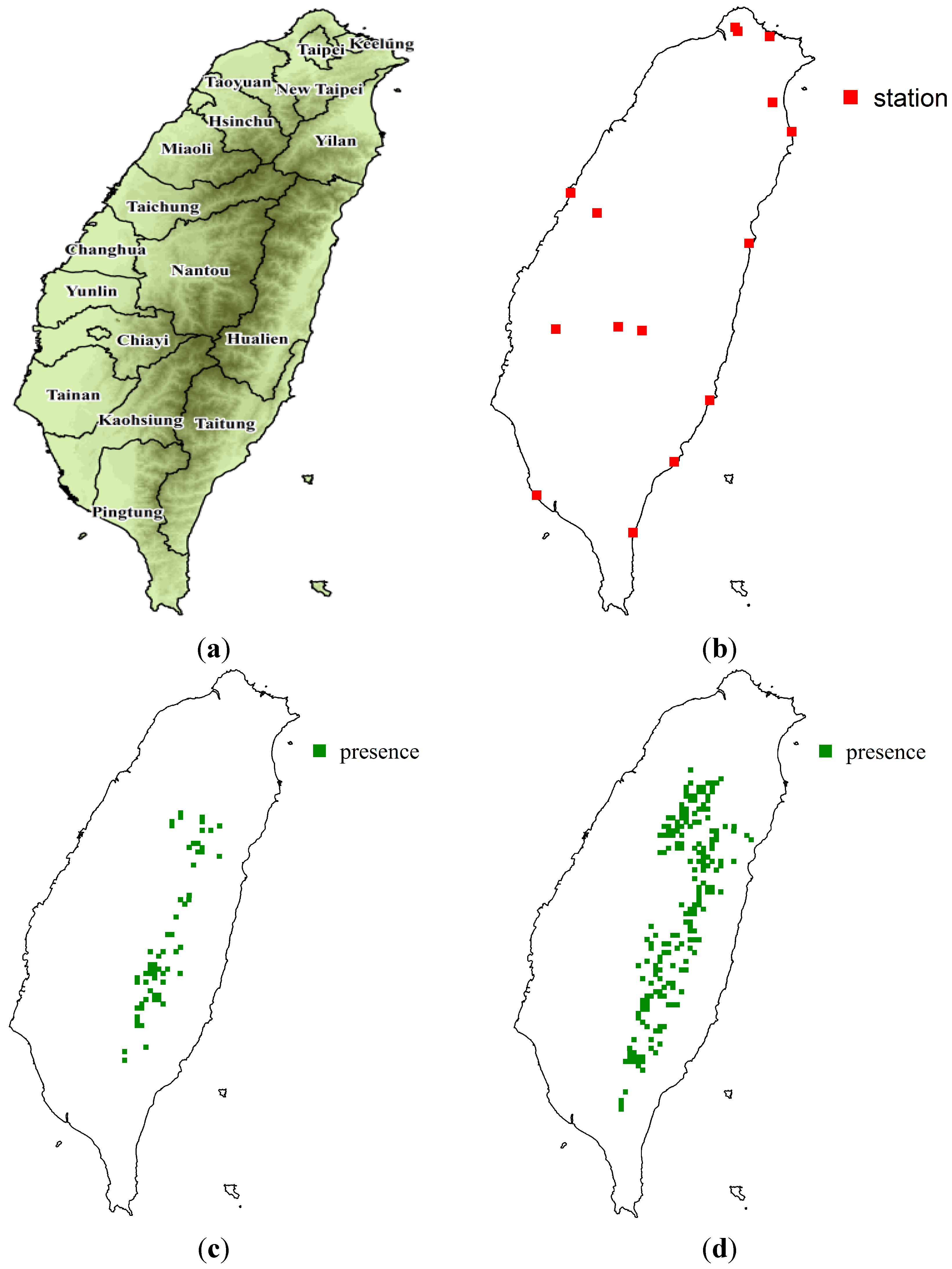
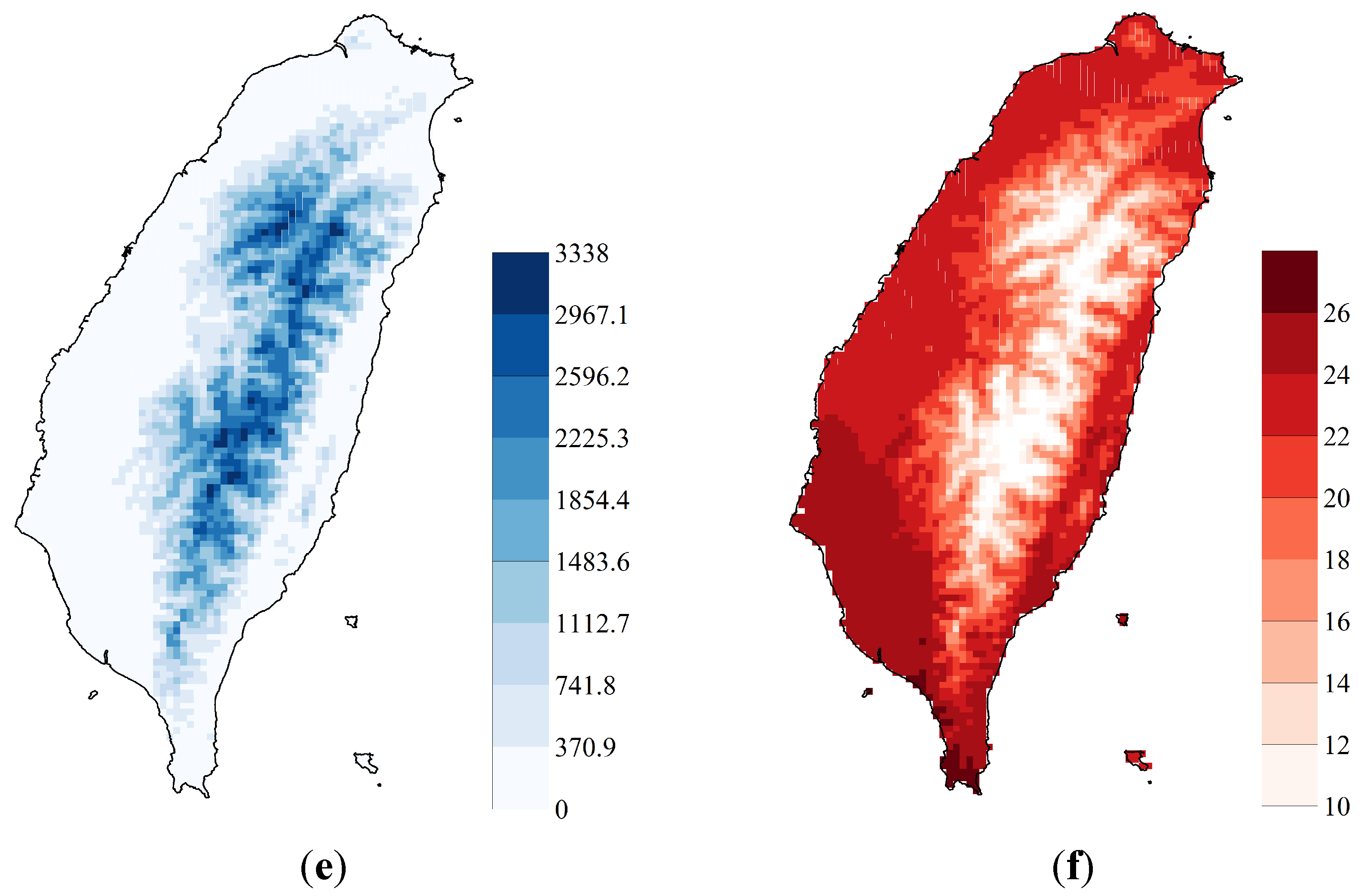
2.1. Study Area and Sampling Data

Taiwan is a mountainous island in eastern Asia. It is bisected by the Tropic of Cancer, which divides the island’s climate into tropical monsoon in the south and sub-tropical monsoon in the north. Approximately 60% of the island is comprised of mountainous regions, including the north-south Central Range, the Hsueh Shan Range, and the Yu Shan Range, which contain more than 200 summits over 3000 m in elevation. Due to the complicated geology and mountainous environment, there is a high degree of diversity in vegetation. The vegetation of Taiwan can be divided into six zones [45] including the alpine zone, the Abies zone, the Tsuga-Picea zone, the Quercus zone, the Machilus-Castanopsis zone, and the Ficus-Machilus zone, based on the dominant species and climate at different altitudes. The coniferous forests are divided into three zones [45]:
(1)
Alpine vegetation zone (mainly composed of Juniperus squamata forests and scrubs);
(2)
Subalpine coniferous forests (Abies zone);
(3)
Upper montane coniferous forests (Tsuga-Picea zone).
The high-mountain coniferous forest zones are dominated by species such as Abies kawakamii, Tsuga chinensis var. formosana, Picea morrisonicola and Pinus armandii var. mastersiana. Due to the high prevalence of Abies (Abies kawakamii) and Tsuga (Tsuga chinensis var. formosana), these two species were selected as the target species in this study. The Abies species, which is endemic to Taiwan, has an altitudinal range between 3000 m and 3500 m above sea level [46] with a cold and humid environment [47]. Abies, one of the 40 fir species known worldwide, is also endangered. This is possibly due to its specific survival needs, which restrict it to a narrow habitat. This species has received little conservation attention [46]. The ecotone of Abies and Tsuga exists at the lower elevations around 3000 m. The Tsuga is widely distributed on moist north facing slopes at 2500–3100 m elevation; and it is mixed with Chamaecyparis formosensis and C. obtusa var. formosana in the prevalent cloud forests around 1800–2400 m. In the northern part of the island, which is affected by the northeastern monsoon, the lower limit of Tsuga is approximately 1500 m.
We compiled the raw dataset used in this study from the Third Forest Resources and Land Use Inventory in Taiwan (TFRLUI) published by the Forestry Bureau in the Council of Agriculture [48]. The inventory data, from 1990 to 1995, included land-use types, forest types, timber, animal resources and soil types. The investigation of each forest plot involved systematic sampling every three kilometers from the starting point at 121.5135° E, 25.03534° N. A total of 3996 ground plots were selected from aerial photos of the national forests. For this study, vegetation raster cells, currently classified as sustaining an Abies and/or a Tsuga population, were chosen for modeling. All forests’ survey data (Figure 1c,d) were used for predicting spatial distributions based on various climate scenarios from different GCMs.
In this study, the five GCMs, CSIRO-Mk3.5 (CS), GFDL-CM2.1 (GF), MIROC3.2 (medres) (MI), MPI-ECHAM5 (MP), and MRI-CGCM2.3.2a (MR), and three greenhouse gas emissions scenarios, B1, A1B, and A2, were adopted to represent different temperature sensitivities for the period 2020–2039 [49]. Unfortunately, GCMs output data has a horizontal resolution between 250 and 600 km; since SDMs generally require a grid resolutions on the order of 1–5 km2 [50], the direct application of SDMs on GCM output data is rarely possible. The original GCMs output data for 2020–2039 was downscaled to the resolution of 25 km × 25 km by the Taiwan Climate Change Projection and Information Platform (TCCIP), and then was downscaled to the resolution of 3 km ×3 km (Figure 1f) by Area-to-Point (ATP) co-kriging and validated through the use of weather station networks from the Central Weather Bureau (Figure 1b) and a high resolution digital elevation model (Figure 1e) [51,52].
Figure 1. (a) The topography of Taiwan; (b) locations of weather stations; (c) sample sites (presence-only) for Abies; (d) sample sites (presence-only) for Tsuga; (e) elevation data from a digital elevation model; (f) downscaled annual temperature data for 2020–2039.
Forests 05 02882 g001aForests 05 02882 g001b

2.2. Maximum Entropy

The distributions of the focal species were estimated by maximum entropy based on the site where the species were recorded and the correlating background environmental variables (driving factors). A logistic regression analysis using SPSS (Statistical Package for the Social Sciences, SPSS Inc., Chicago, IL, USA) identified the environmental variables with greatest influence on distribution, which were then used in the SDMs. The candidate variables included: moisture, precipitation, slope, aspect, elevation, and temperature. However only four significant environmental variables were identified by the logistic regression, and subsequently used in this study: average annual temperature, average spring monthly temperature, average summer monthly temperature, and elevation. Though precipitation is often a crucial factor determining tree species distribution, for mountainous regions of Taiwan, where annual precipitation often exceeds 3000 mm, from the macroscopic prospective this may not be a limiting factor in most regions of our study area. Aspect is also an environmental factor which is often crucial to tree species distribution. However, in relatively low latitude regions, such as Taiwan, aspect may not be as important compared to high latitude regions, especially when considering the humid conditions intrinsic to Taiwan. Our field experience substantiates the findings of our logistic regression model because distributions of both Abies kawakamii and Tsuga chinensis var. formosana were observed across large ranges which span both steep slopes and valleys, indicating that their distribution is predominantly determined by macro-climate environmental factors such as temperature.
Following Dudík et al. (2007), an unknown probability distribution π(x) over a space X across the entire study area was estimated, and the presence records were used to determine a set of constraints that were likely to be satisfied by π(x) [53]. The focal species were only present at certain locations in the set of location samples ( x 1 , , x m ), each of which corresponds to specific environmental variables. The expected value π [ z ] of z , selected environment variables, under the distribution π is defined as:
π [ z ] = x X π ( x ) z ( x )
where X is the entire study area.
Since the empirical average of z ( π ̃ [ z ] ) and the expectation of z ( p [ z ] ) are both very close to its true expectation ( π ̃ [ z ] π [ z ] and p [ z ] π [ z ] ) [54], many distributions p ( x ) satisfy the constraint p [ z ] π [ z ] however the p ( x ) whose entropy is largest should be chosen. The entropy of p ( x ) is defined as follows [54]:
Maximize
H ( p ) = x X p ( x ) l n p ( x )
Subject to
| p [ f ] π ̃ [ f ] | β
where β is the estimated upper bound (tolerance) of how close p [ f ] is to π ̃ [ z ] (the empirical distribution of the focal species). The p ( x ) can be written as the following function (Gibbs model):
p ( x ) = exp ( j = 1 n λ j z j ( x ) ) x X exp ( j = 1 n λ j z j ( x ) )
where λ j is the coefficient of jth environmental variables (features) z j .

2.3. The Bootstrapping Method

2.3.1. Evaluating Data and Model Performance

The bootstrapping method was implemented by randomly selecting 80% of the presence records from the survey data used to estimate the distribution of focal species by the maximum entropy method. The remaining 20% of the presence data were used as a test dataset and applied to validate the performance by computing the area under the receiver operating characteristic curve (AUC) value. This procedure was done iteratively creating 1000 maximum entropy species distribution models and corresponding validation AUC values.

2.3.2. The Confidence Region of SDM Parameters

The ellipsoidal confidence regions, which are generalizations of univariate symmetrical confidence intervals, for the coefficients of the environmental variables in the maximum entropy model, λ j , are generated by using the nonparametric bootstrapping procedure [55]. The confidence regions can be written as the following equation [55]:
R = { θ ̂ Ω ̂ × r : r R α }
where R α is any region such that P [ Ω ̂ × ( θ θ ̂ ) R α ] = α and α was set to 0.95. The shape of the region R depends on the shape of the region R α , which is ellipsoid in this study.

2.4. Variability Analysis

Uncertainties intrinsic to future species distribution models based on future climate models are many and varied [38,39,40,41]. Although it has been demonstrated that SDMs contribute significantly to the total variability of future species distribution projections [22,60], the overall uncertainty in suitable future habitats arising from this variability has rarely been considered [56,57,58,59,60]. In order to enhance the reliability of projections, it is necessary to quantify the uncertainty from several sources. In this way, we can construct an ensemble of relatively reliable forecasts [61].
In this study, the SDM model variability arising from three different sources of uncertainty, including SDM parameters, GCMs and GESs was quantified. Evaluation of relative variability originating in SDM parameters was undertaken by randomly generating 1000 sets of coefficients via a sample presence bootstrapping technique. Coefficients falling within the 95% confidence range were then compared with those coefficients falling outside of the confidence range. The Wilcoxon test was adopted in this study to identify the significant differences in elevation of projected suitable habitats for the two focal species, under 15 future scenarios (5 GCM × 3 GES) and the baseline scenario, based on the parameters from 1000 sets of coefficients. This procedure led to a factorial design which crossed 1000 sets of the SDM’s coefficients, five GCMs and three GESs, thus resulting in 15,000 different projections of future distribution for each species. Based on this design, the proportion of the three different sources of uncertainty, GCM, GES, and SDM model’s parameters, were quantified using a general linear model, which was assessed by calculating the ratio between the deviances explained by each source against the null deviance [41].
Besides the sources of uncertainties, the local and spatial uncertainties were also quantified in this study. The local uncertainty at location k ( P l k ) can be defined by the following equation [62]:
P l k = n p ( g k ) / 1000
where 1000 is the number of realizations, and n p ( g k ) is the number from the 1000 realizations in which the simulated species were present at location k.
The joint probability (Pj, global uncertainty) in m occurrence locations ( u 1 , u 2 , u 3 , u m ) was written as follows [63,64]:
P j = n p ( u 1 , u 2 , u 3 , u m ) / 1000
where 1000 is the number of realizations, and n p ( u 1 , u 2 , u 3 , u m ) is the number from the 1000 realizations in which the simulated species were present at m locations; m is the number of cells, out of 1000 realizations, in which the given critical probability, or cutoff point that could be viewed as the given minimal habitat suitability threshold, is satisfied; np is the number of realizations, out of 1000, whose projected focal species distributions are entirely within the given critical probability area.

2.5. Identifying Protected Areas

Zonation is a systematic conservation planning decision support tool. It generates a hierarchy of conservation priorities over all cells in a landscape based on their conservation value [65]. We used Zonation to delineate protected areas for the modeled species under the baseline and the climate change scenarios. The selections were made based on occurrences of conservation targets and pseudo targets, which represent the possible occurrences of target species following distribution predictions. In core-area Zonation, cell removal is done in a manner that minimizes biological loss by picking cell i that has the smallest δ:
δ i = M a x j Q i j ( S ) w j c i
where wj is the weight (or priority) of species j and ci is the cost of adding cell i to the reserve network [66]. The critical part of the equation is Qij(S), which is the proportion of the remaining distribution of species j located in cell i in the remaining set of cells, S. When a part of the distribution of a species is removed, the proportion located in each remaining cell increases.
We then computed an index which integrates both the estimated habitat suitability and conservation status, as indicated by Zonation, to identify cells of greatest suitability for Abies and Tsuga within a protected area network under 15 future scenarios and the baseline scenario. The matching of climate suitability with conservation area for species r , in a given grid cell w , can be expressed as ( S w r ) [67]:
S w r = H S w r × C A w
where H S w r is the suitability score of grid cell w for a given species   r , and C A w is 1, if the grid cell w was selected for protection; otherwise, C A w is 0. The S w r ranges from 0, for grid cells which are unsuitable for species or are not selected for conservation, to 1, for grid cells which have both high suitability for the focal species and are also selected for conservation. The habitat suitability within protected areas for species  r over the study area can be written as the following equation:
S r = w = 1 N S w r
where N is the number of grid cells in the study area. Moreover, the proportions of habitat suitability covered by protected areas for species r , ( C P r ), can be expressed as:
C P r = S r / w = 1 N H S w r
Large C P r values correspond to large protected area networks which possess a large number of high quality habitat cells.

3. Results and Discussion

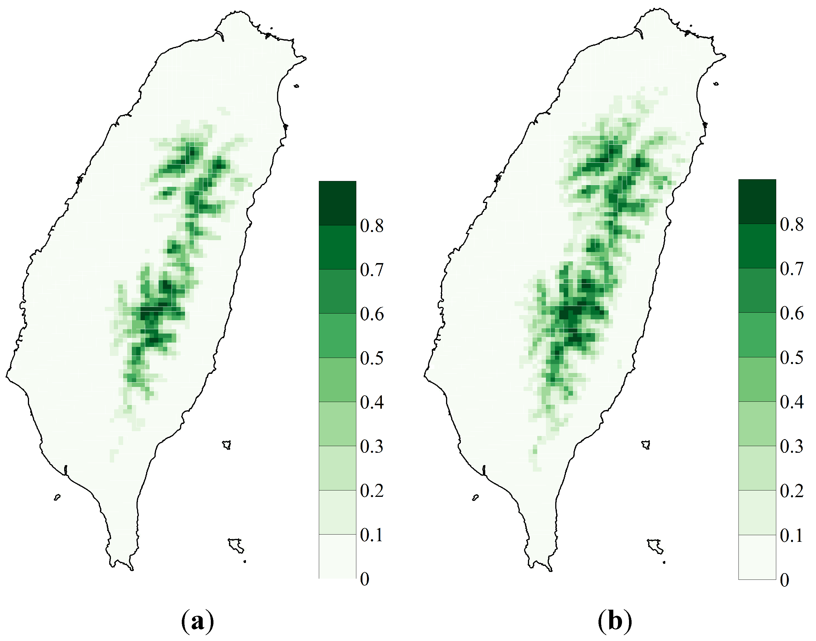
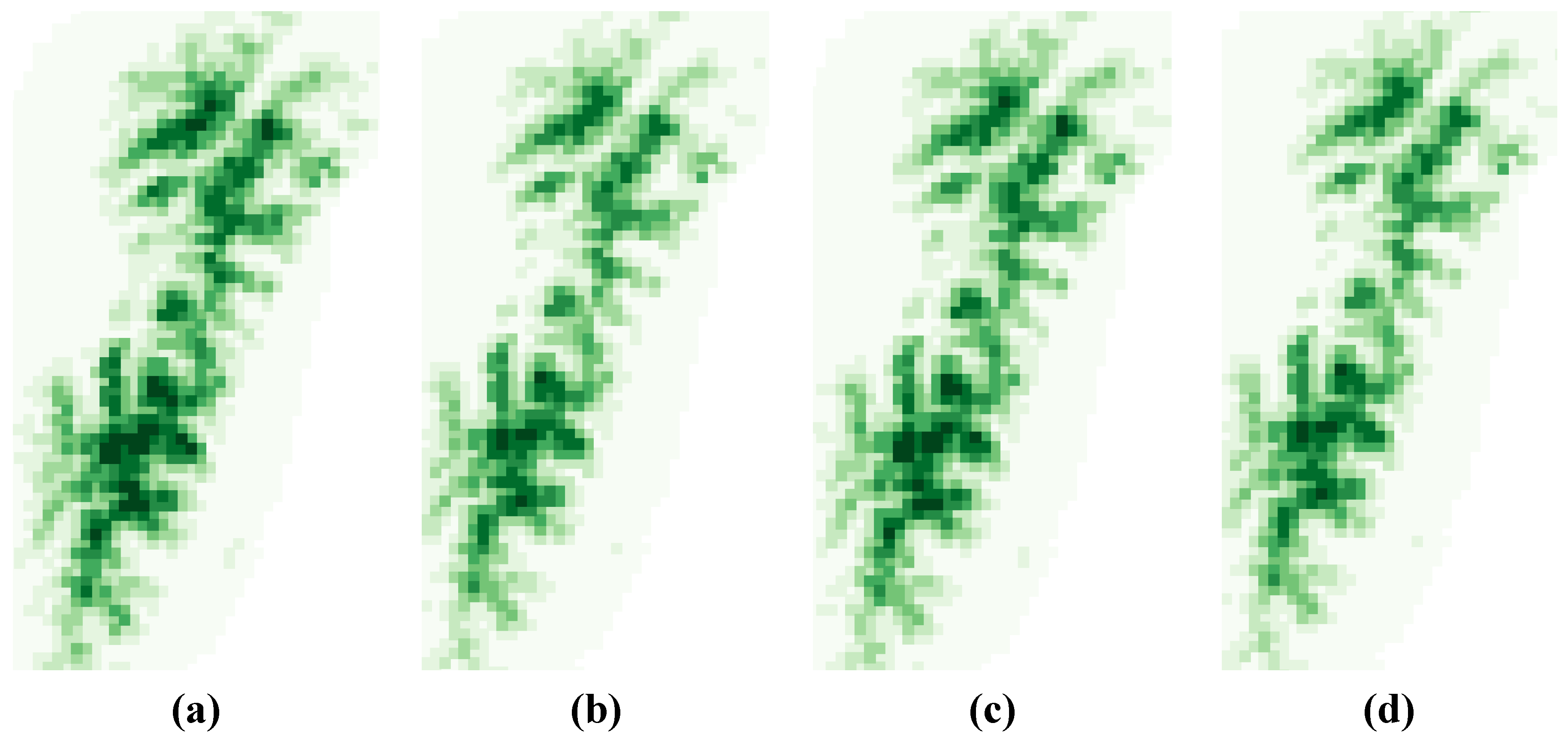
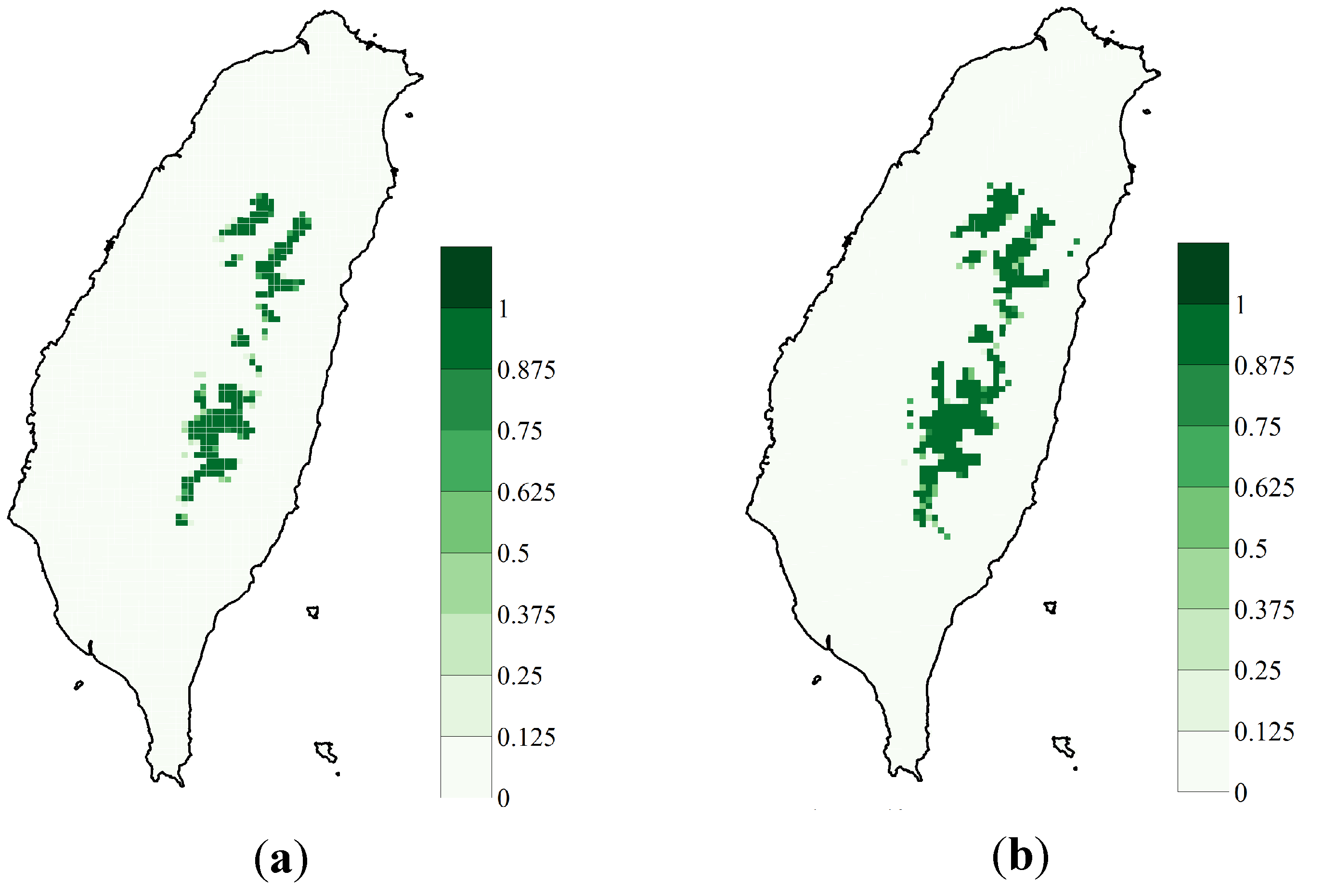
3.1. SDM Performance, Focal Species Distribution and Their Shifts in Elevation

The validation AUC values calculated from 1000 iterations of our SDM range from 0.8 to 0.96 for Abies and from 0.85 to 0.95 for Tsuga. The mean and the standard deviation of the 1000 AUC values are 0.88 and 0.021 for Abies and 0.91 and 0.015 for Tsuga. The higher mean AUC value and lower standard deviation correlate with more precise maximum entropy predictions. The high accuracy of the predictions leads to higher consistencies between predicted distributions of focal species and presence data distributions of Abies (Figure 1b and Figure 2a) and Tsuga (Figure 1c and Figure 2b).
Figure 2. The predicted baseline habitat suitability for: (a) Abies; (b) Tsuga.
Forests 05 02882 g002
The trees species future distributions under different scenarios are presented in Figure 3 and Figure 4. The distributions are slightly different for the two species; however, the SDMs reveal that the species prefer to live in areas with low temperatures and high altitudes.
Figure 3. Predicted habitat suitability in Central Mountain Range area for Abies in 12 future scenarios (3 GES × 2 GCM × 2 parameter) for 2020–2039.
Forests 05 02882 g003aForests 05 02882 g003b
Figure 4. Predicted habitat suitability in Central Mountain Range area for Tsuga in 12 future scenarios (3 GES × 2 GCM × 2 parameter) for 2020–2039.
Forests 05 02882 g004aForests 05 02882 g004b

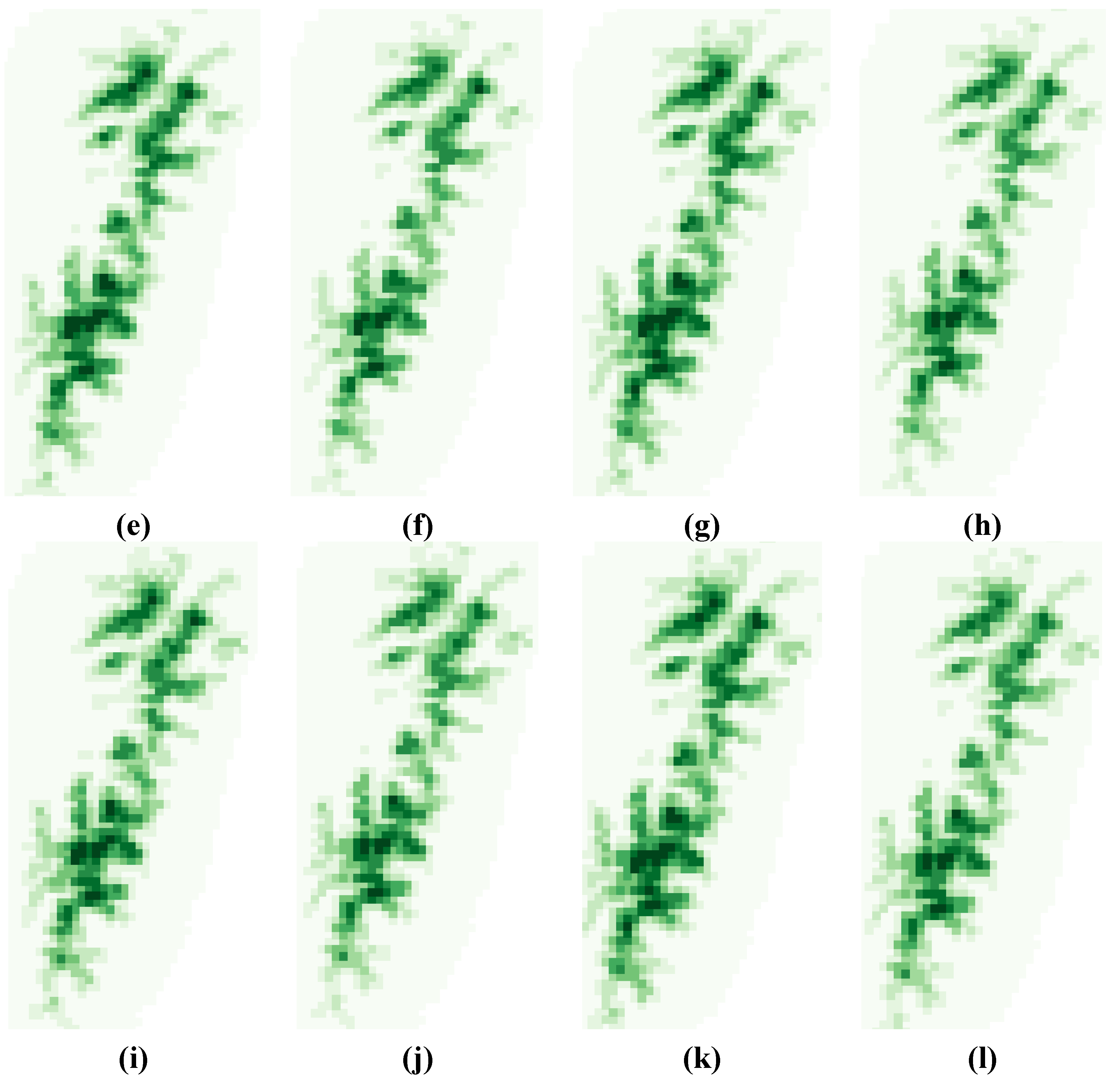
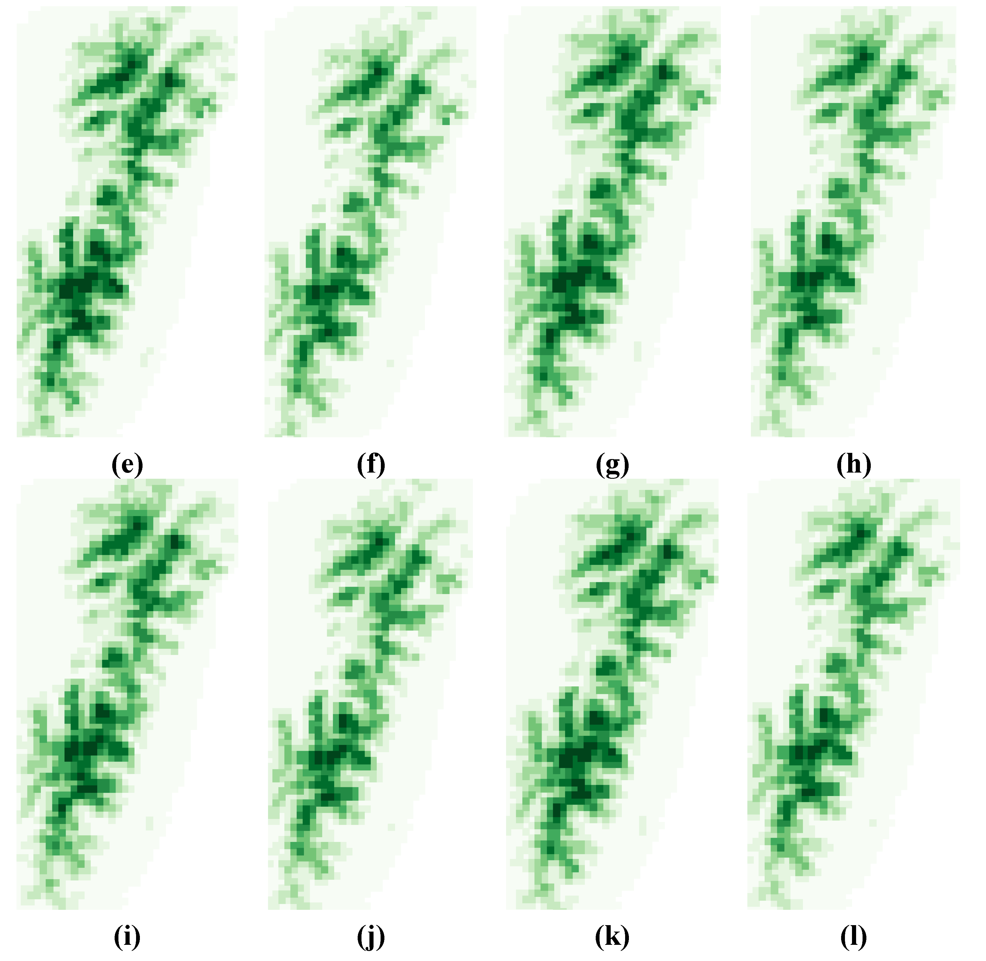
3.2. Variability Analysis

The discrepancies in results of species habitat shifts with constant GCMs and GESs were interpreted as the uncertainty introduced by maximum entropy model parameters. The distribution of coefficients of the environmental variables in the maximum entropy model for Abies and Tsuga, which are elevation, average annual temperatures, average spring monthly temperatures and average summer monthly temperatures, based on bootstrap resampling are shown in Figure 5. For Abies, they are in the range of 0.29 to 4.70, −3.42 to −1.19, −2.02 to 1.11, and −4.59 to −0.97, respectively. For Tsuga, they are in the range of −1.26 to 1.61, −3.29 to −1.98, −2.57 to −0.31, and −3.49 to −1.20, respectively. The dashed lines in Figure 5 show the SDM’s parameters fitted by the original data, which approximate the mean parameters of 1000 sets of bootstrap resampling data indicating the low bias of the estimated parameters. For evaluating the variability of parameters, 1000 sets of coefficients which were within the 95% bootstrap confidence interval were used to estimate the future distribution of the modeled species. The nonparametric Wilcoxon test was then used to identify significant differences in habitat elevation between the baseline scenario versus each future scenario (Table 1). The shifts in elevation were based on species current distribution, and the significant environmental variables which these distributions correspond to.
Figure 5. The bootstrap histogram of the coefficients in maximum entropy model for Abies: (a) elevation; (b) average annual temperature; (c) average monthly spring temperature; (d) average monthly summer temperature, and for Tsuga: (e) elevation; (f) average annual temperature; (g) average monthly spring temperature; (h) average monthly summer temperature. The blue line is the fitted kernel density.
Forests 05 02882 g005
According to the results of predicted temperature data from different GCMs and GESs (Table 1), greater temperature increases correlate with a higher “count”, which represents the number of statistically significant differences in habitat elevation under baseline and future climate scenarios in 1000 SDM outputs. Moreover, a higher “count” indicates a greater reliability in predicting the upward shift in focal species distribution. The homogeneity of the “count” between the 15 scenarios was tested using the chi-square test, which contrasts the non-homogeneity of the “count” between the 15 scenarios (p value < 0.0001) for each species. The “count” under scenarios 2, 3, 6, 7, 8, 11 and 13 for Abies and scenarios 1, 2, 3, 6, 7, 8, 11 and 13 for Tsuga are significantly higher (+) than that under other scenarios (Table 1). In addition, scenario 8 has the largest “count” for Abies (668) and Tsuga (841). The highest average annual temperatures and average summer monthly temperatures in scenario 8 lead to the most drastic upward shift in distribution for both species. As for other scenarios, the temperature in scenario 2, 3, 6, 7, 11 and 13 all increase leading to a higher “count” for each species. Moreover, as can be seen from Table 1 as the “count” approaches extreme values, which are 0 or 1000, only slight variability of parameters in the maximum entropy model are observed. The scenarios with large variability from parameters in predicting the upward shift of the focal species distributions are scenarios 2, 6 and 13 for Abies and scenarios 1, 2 and 7 for Tsuga. This result indicates that the intermediate increments of temperature change lead to the highest variability in SDM parameters. In other words, we have higher confidence when predicting the upward shift of tree species under scenarios which project larger increments of temperature change.
Table 1. The difference in temperature under each climate change scenario (for 2020–2039) in comparison to the baseline scenario, and the number of statistically significant differences in the optimal elevation of focal species habitat in 1000 different sets of outputs, which are contained in the 95% bootstrap confidence interval.
ScenarioGESGCMChange of Average Temperature (°C)Significant Shift in Elevation of Habitat
AnnualSpringSummerAbiesTsuga
CountUncertaintyCountUncertainty
1B1CS0.771.030.75193 (−)0.16489 (+)0.25
2GF0.880.760.93466 (+)0.25571 (+)0.25
3MI1.021.220.93576 (+)0.24805 (+)0.16
4MP−0.03−0.06−0.20 (−)0.000 (−)0.00
5MR0.340.170.590 (−)0.002 (−)0.00
6A1BCS0.881.171.02514 (+)0.25722 (+)0.20
7GF0.840.520.82341 (+)0.23442 (+)0.25
8MI1.091.081.07668 (+)0.22841 (+)0.13
9MP−0.03−0.06−0.20 (−)0.000 (−)0.00
10MR0.380.330.673 (−)0.0029 (−)0.03
11A2CS0.781.130.89355 (+)0.23589 (+)0.24
12GF0.670.690.79149 (−)0.13368 (0)0.23
13MI0.911.290.91489 (+)0.25757 (+)0.18
14MP−0.03−0.06−0.20 (−)0.000 (−)0.00
15MR0.350.310.510 (−)0.001 (−)0.00
Note: The symbols (+), (0) and (−) represent the “count” as being significantly higher than, equal to, and significantly lower than expected based on the chi-square test; GES: Greenhouse Gas Emissions Scenarios; GCM: General Circulation Model; CS:CSIRO-Mk3.5; GF: GFDL-CM2.1; MI : MIROC3.2 (medres); MP : MPI-ECHAM5 (MP); MR : MRI-CGCM2.3.2a.
The variability in projecting future species distributions does not only originate from SDM parameters but also arises from GCMs and GESs [59,61]. The outputs of all GCM × GES combinations cover a wide range of potential future climate conditions; thus, the need to evaluate the variability from both GCMs and GESs is increasing [41]. The variability arising from the three uncertainty sources analyzed in this study, GCMs, GESs, and bootstrapped parameters, are listed in Table 2. The proportions of variability are estimated by calculating the ratio between the deviance explained by one source and the null deviance with the generalized linear model based on 15,000 different future projections for each species [41]. Due to the high variation of increasing temperature between each GCM based on the same GES, the contributions of GCMs, which are 31.3% for Abies and 42.8% for Tsuga, are significantly higher than that of GESs, which are 0.9% for Abies and 0.2% for Tsuga. This result is consistent with that of the “count” in five GCMs based on the same GES which are significantly different from one another in Table 1. This implies that a high level of variability between different GCMs exists, and that this variability affects predictions of future species habitat distributions.
Table 2. Proportion of variability from three different uncertainty sources, including model parameters, GCMs and GESs.
Source of UncertaintyContribution (%)
parameters67.9
AbiesGCMs31.3
GESs0.9
parameters57
TsugaGCMs42.8
GESs0.2
In contrast, the proportions of variability originating from GESs are small because, all else being equal, the predicted temperatures under the three GESs are similar. This result corroborates the studies by both Stott & Kettleborough (2002) and Buisson et al. (2010), who found that the variability from different GESs is small [41,68]. On the other hand, the proportion of variability in predicting upward shifts of tree species originating from SDM parameters is quite large, being 67.9% for Abies and 57.0% for Tsuga. This means that the variability from the model's parameters has a strong effect on predicting the shift of focal species. This result is in accordance with the study by Buisson et al. (2010), who suggested that the high proportions of the total variability in future projections are from SDMs [41]. In summary, the above findings suggest that variability originating from both SDM parameters and GCMs should be of first concern as they contribute most to the total variability in predicting the upward shift of focal species.

3.3. Local and Global Uncertainties

Figure 6 shows the proportion of habitat in 1000 realizations under the baseline scenario for Abies and Tsuga, which provides a measure of local uncertainty associated with a single location (grid). Under each scenario, the areas with high (95%) habitat coverage were located in the center of Taiwan where the central mountain range is located. As for the global uncertainty, given a critical probability of species occurrence, a higher joint probability means greater reliability (lower global uncertainty) of the mapped locations of species occurrences. The joint probabilities increase with the critical probability under each scenario (Table 3). Kerry et al. (2010) and Goovaerts (2009) suggest the critical probabilities 75% and 90% are enough to generate a reliable joint probability. In this study, the joint probabilities under each scenario are larger than 0.5 when the critical probability reaches 0.75 [63,69].
Table 3. The global uncertainty under baseline and 15 future scenarios.
Cut-offAbiesTsuga
Scenario 0.70.750.80.850.90.950.70.750.80.850.90.95
B0.430.580.650.70.780.90.430.580.650.70.780.9
s10.490.560.620.720.820.890.490.560.620.720.820.89
s20.450.540.650.730.820.910.450.540.650.730.820.91
s30.470.620.660.730.830.910.470.620.660.730.830.91
s40.420.520.690.740.790.880.420.520.690.740.790.88
s50.460.540.660.710.80.920.460.540.660.710.80.92
s60.450.510.670.720.840.910.450.510.670.720.840.91
s70.440.530.590.770.810.890.440.530.590.770.810.89
s80.550.60.670.740.810.890.550.60.670.740.810.89
s90.420.520.690.740.790.880.420.520.690.740.790.88
s100.480.540.620.720.810.910.480.540.620.720.810.91
s110.50.530.660.750.820.90.50.530.660.750.820.9
s120.470.530.620.740.860.910.470.530.620.740.860.91
s130.450.520.680.740.830.910.450.520.680.740.830.91
s140.420.520.690.740.790.880.420.520.690.740.790.88
s150.460.560.640.70.820.90.460.560.640.70.820.9
Figure 6. The proportion of habitat in 1000 realizations (local uncertainty) under the baseline scenario for: (a) Abies; (b) Tsuga.
Forests 05 02882 g006

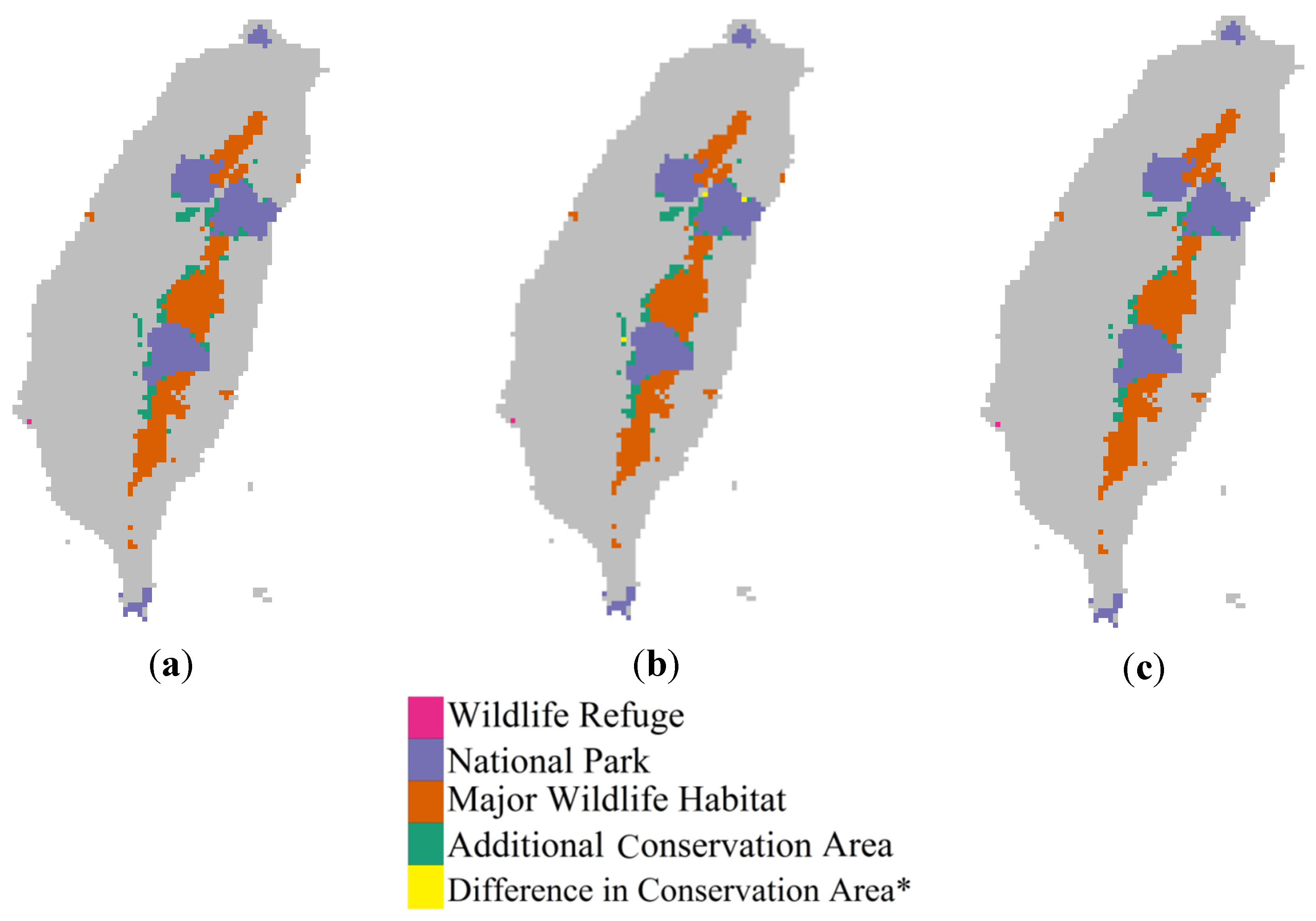
3.4. Implications for Protected Areas

Only a limited number of conservation planning studies have taken the effects of climate change into account. However, climate change can induce rapid shifts of species distribution resulting in existing protected areas no longer ensuring the long-term persistence of certain species [36,67]. In this study, for Abies and Tsuga, the climate suitability (S) and the climate suitability within protected areas (Scons), including Taiwan National Parks, Taiwan Wildlife Refuges, and Taiwan Major Wildlife Habitats are likely to decrease under most future scenarios (Table 4). However, the proportions of suitable habitat protected for Abies and Tsuga under the baseline and 15 future climate scenarios are very similar to each other, which are 87.2%–90.9% and 85.3%–88.7% for Abies and Tsuga, respectively. This result is not consistent with previous studies’ concern that climate change may lead to the failure of protected areas to cater to the needs of focal species [36,67,70,71,72]. In our study area, despite the shrinkage of focal species habitat under many of the future scenarios, the existing conservation areas are still adequate. In fact, the proportions of species habitat protected under many of the future climate scenarios increase in comparison to the baseline scenario as reduced total area of suitable habitat force species into conservation areas.
Table 4. Total habitat suitability (S) and habitat suitability within protected areas (Scons) and the proportion of suitable habitat under existing protected areas (CP) under baseline and 15 future climate scenarios (for 2020–2039) for Abies and Tsuga.
ScenarioSAbies SconsCP (%)STsuga SconsCP (%)
B199.7174.287.2295.3252.885.6
145.4161.6 90226.2199.688.2
s2155.6140.690.4221.9196.388.5
s3152.8138.490.6211.7187.788.7
s4207.0179.786.8305.5260.785.3
s5175.5155.888.8258.7223.686.4
s6154.3139.690.5215.4190.988.6
s7159.5143.890.1230.2202.588
s8149.6136.090.9209.2185.588.7
s9207.0179.786.8305.5260.785.3
s10172.3153.589252.0218.386.7
s11158.2142.790.2220.8195.488.5
s12163.0146.489.8233.3204.887.8
s13155.1140.290.4214.1189.888.6
s14207.0179.786.8305.5260.785.3
s15176.7156.788.7257.7222.886.5
Nonetheless, new protected areas can play an important role in protecting Abies and Tsuga under climate change. In most of our climate change scenarios the proportion of suitable habitat covered by existing protected areas is higher than the baseline scenario because the total area of future suitable habitat declines. As such, increasing protected areas as determined by Zonation will be necessary to offset the loss of suitable habitat [71] (Figure 7). The additional area to be protected depends on the level of climate change. Therefore the union of all areas suitable under the 15 climate change scenarios and not currently protected would be optimal in establishing the most robust conservation area (Figure 7b). Interestingly, when considering the worst case scenario, that is the one which projects the largest increment of temperature change, a smaller protected area is identified in comparison to that correlating to all 15 climate change scenarios (Figure 7c).
Figure 7. Current protected areas in Taiwan, including Wildlife Refuges, National Parks and Major Wildlife Habitats, and the additional areas determined by Zonation which are currently outside of existing protected areas: (a) under baseline; (b) all future climate scenarios (the extra conserved area under future climate scenario is the union of that under 15 future scenarios); and (c) future climate scenario (the worst scenario with the largest increase of temperature). Note: * The difference in additional conservation area between baseline and future climate scenarios. The period of future climate scenario is for 2020–2039.
Forests 05 02882 g007

4. Conclusions

The upward shift of mountainous and alpine habitats is expected under climate change. In Taiwan, an island that is 60% mountainous, the high elevation habitats will be directly influenced by increasing temperatures. In this study, the ensemble forecasting framework used to predict shifts in elevation of Abies and Tsuga habitats allowed for more robust decisions in conservation planning by taking multiple sources of variability into account, namely: SDM parameters, GCMs and GESs. The findings indicate that the projected shift in elevation of each species habitat differs among climate change models and among 1000 SDM realizations based on different sets of parameters. To a lesser degree, variability in predictions originating from different emission scenarios was also found to contribute to overall uncertainty. Our results show that most of the variability originates from the model’s parameters as well as the GCMs, indicating that uncertainty has a strong influence on predicting the shift of the modeled species distribution. Although most of the climate change induced shrinkage of habitats is already covered by existing protected areas, in order to offset the loss of suitable habitat and reduce uncertainties caused by climate change, we suggest additional habitat be added to the network of protected areas.

Acknowledgments

The authors would like to thank the Ministry of Science and Technology of the Republic of China, Taiwan, for financially supporting this research under Contracts Nos. 103-2119-M-002-012 and 101-2923-I-002-001-MY2. Tzung-Su Ding helped compile the environmental variables instrumental to this study.

Author Contributions

The scope of this study was developed by Yu-Pin Lin and Wei-Chih Lin. The sampling data of Abies and Tsuga were provided by Cheng-Tao Lin and Chyi-Rong Chiou. The data analysis, simulation of SDM models and uncertainty analyses were conducted by Wei-Chih Lin with the supervision of Yu-Pin Lin and Wan-Yu Lien. The first manuscript draft was written by Wei-Chih Lin and was substantially revised by Wan-Yu Lien, Yu-Pin Lin, Neville D. Crossman, Johnathen Anthony, Cheng-Tao Lin and Chyi-Rong Chiou.

Conflicts of Interest

The authors declare no conflict of interest.

References

  1. Lindner, M.; Maroschek, M.; Netherer, S.; Kremer, A.; Barbati, A.; Garcia-Gonzalo, J.; Seidl, R.; Delzon, S.; Corona, P.; Kolström, M. Climate change impacts, adaptive capacity, and vulnerability of european forest ecosystems. For. Ecol. Manag. 2010, 259, 698–709. [Google Scholar] [CrossRef]
  2. Gonzalez, P.; Neilson, R.P.; Lenihan, J.M.; Drapek, R.J. Global patterns in the vulnerability of ecosystems to vegetation shifts due to climate change. Glob. Ecol. Biogeogr. 2010, 19, 755–768. [Google Scholar] [CrossRef]
  3. Rosenzweig, C.; Karoly, D.; Vicarelli, M.; Neofotis, P.; Wu, Q.; Casassa, G.; Menzel, A.; Root, T.L.; Estrella, N.; Seguin, B. Attributing physical and biological impacts to anthropogenic climate change. Nature 2008, 453, 353–357. [Google Scholar] [CrossRef] [PubMed]
  4. Parry, M.L. Climate change 2007: Impacts, adaptation and vulnerability: Contribution of working group ii to the fourth assessment report of the intergovernmental panel on climate change; Cambridge University Press: Cambridge, UK, 2007; Vol. 4. [Google Scholar]
  5. Solomon, S. Climate change 2007: The physical science basis: Working group i contribution to the fourth assessment report of the ipcc; Cambridge University Press: Cambridge, UK, 2007; Vol. 4. [Google Scholar]
  6. Martin, T.E. Abiotic vs. biotic influences on habitat selection of coexisting species: Climate change impacts? Ecology 2001, 82, 175–188. [Google Scholar] [CrossRef]
  7. Bykova, O.; Chuine, I.; Morin, X.; Higgins, S.I. Temperature dependence of the reproduction niche and its relevance for plant species distributions. J. Biogeogr. 2012, 39, 2191–2200. [Google Scholar] [CrossRef]
  8. Guisan, A.; Zimmermann, N.E. Predictive habitat distribution models in ecology. Ecol. Model. 2000, 135, 147–186. [Google Scholar] [CrossRef]
  9. Randin, C.F.; Engler, R.; Normand, S.; Zappa, M.; Zimmermann, N.E.; Pearman, P.B.; Vittoz, P.; Thuiller, W.; Guisan, A. Climate change and plant distribution: Local models predict high-elevation persistence. Glob. Chang. Biol. 2009, 15, 1557–1569. [Google Scholar] [CrossRef]
  10. Gehrig-Fasel, J.; Guisan, A.; Zimmermann, N.E. Tree line shifts in the swiss alps: Climate change or land abandonment? J. Veg. Sci. 2007, 18, 571–582. [Google Scholar] [CrossRef]
  11. Grabherr, G.; Gottfried, M.; Gruber, A.; Pauli, H. Patterns and current changes in alpine plant diversity. In Arctic and Alpine Biodiversity: Patterns, Causes and Ecosystem Consequences; Springer: Heidelberg, Berlin, Germany, 1995; pp. 167–181. [Google Scholar]
  12. Vittoz, P.; Jutzeler, S.; Guisan, A. Flore alpine et réchauffement climatique: Observation de trois sommets valaisans à travers le 20ème siècle. Bull. Murithienne 2006, 123, 49–59. [Google Scholar]
  13. Walther, G.R.; Beißner, S.; Burga, C.A. Trends in the upward shift of alpine plants. J. Veg. Sci. 2005, 16, 541–548. [Google Scholar] [CrossRef]
  14. Erschbamer, B.; Kiebacher, T.; Mallaun, M.; Unterluggauer, P. Short-term signals of climate change along an altitudinal gradient in the south alps. Plant Ecol. 2009, 202, 79–89. [Google Scholar] [CrossRef]
  15. Klanderud, K.; Birks, H.J.B. Recent increases in species richness and shifts in altitudinal distributions of norwegian mountain plants. Holocene 2003, 13, 1–6. [Google Scholar] [CrossRef]
  16. Le Roux, P.C.; McGeoch, M.A. Changes in climate extremes, variability and signature on sub-antarctic marion island. Clim. Chang. 2008, 86, 309–329. [Google Scholar] [CrossRef]
  17. Walther, G.-R.; Post, E.; Convey, P.; Menzel, A.; Parmesan, C.; Beebee, T.J.; Fromentin, J.-M.; Hoegh-Guldberg, O.; Bairlein, F. Ecological responses to recent climate change. Nature 2002, 416, 389–395. [Google Scholar] [CrossRef] [PubMed]
  18. Felde, V.A.; Kapfer, J.; Grytnes, J.A. Upward shift in elevational plant species ranges in Sikkilsdalen, Central Norway. Ecography 2012, 35, 922–932. [Google Scholar] [CrossRef]
  19. Hengl, T.; Sierdsema, H.; Radović, A.; Dilo, A. Spatial prediction of species’ distributions from occurrence-only records: Combining point pattern analysis, enfa and regression-kriging. Ecol. Model. 2009, 220, 3499–3511. [Google Scholar] [CrossRef]
  20. Crossman, N.D.; Bryan, B.A.; Cooke, D.A. An invasive plant and climate change threat index for weed risk management: Integrating habitat distribution pattern and dispersal process. Ecol. Indic. 2011, 11, 183–198. [Google Scholar] [CrossRef]
  21. Franklin, J.; Davis, F.W.; Ikegami, M.; Syphard, A.D.; Flint, L.E.; Flint, A.L.; Hannah, L. Modeling plant species distributions under future climates: How fine scale do climate projections need to be? Glob. Chang. Biol. 2013, 19, 473–483. [Google Scholar] [CrossRef] [PubMed]
  22. Araujo, M.B.; Guisan, A. Five (or so) challenges for species distribution modelling. J. Biogeogr. 2006, 33, 1677–1688. [Google Scholar] [CrossRef]
  23. Diniz-Filho, J.A.F.; Mauricio Bini, L.; Fernando Rangel, T.; Loyola, R.D.; Hof, C.; Nogués-Bravo, D.; Araújo, M.B. Partitioning and mapping uncertainties in ensembles of forecasts of species turnover under climate change. Ecography 2009, 32, 897–906. [Google Scholar] [CrossRef]
  24. Lawler, J.J. Climate change adaptation strategies for resource management and conservation planning. Ann. N. Y. Acad. Sci. 2009, 1162, 79–98. [Google Scholar] [CrossRef] [PubMed]
  25. Peterson, A.T.; Ortega-Huerta, M.A.; Bartley, J.; Sánchez-Cordero, V.; Soberón, J.; Buddemeier, R.H.; Stockwell, D.R. Future projections for mexican faunas under global climate change scenarios. Nature 2002, 416, 626–629. [Google Scholar] [CrossRef] [PubMed]
  26. Guisan, A.; Thuiller, W. Predicting species distribution: Offering more than simple habitat models. Ecol. Lett. 2005, 8, 993–1009. [Google Scholar] [CrossRef]
  27. Barbet-Massin, M.; Thuiller, W.; Jiguet, F. The fate of european breeding birds under climate, land-use and dispersal scenarios. Glob. Chang. Biol. 2012, 18, 881–890. [Google Scholar] [CrossRef]
  28. Braunisch, V.; Suchant, R. Predicting species distributions based on incomplete survey data: The trade-off between precision and scale. Ecography 2010, 33, 826–840. [Google Scholar] [CrossRef]
  29. Broennimann, O.; Fitzpatrick, M.C.; Pearman, P.B.; Petitpierre, B.; Pellissier, L.; Yoccoz, N.G.; Thuiller, W.; Fortin, M.J.; Randin, C.; Zimmermann, N.E. Measuring ecological niche overlap from occurrence and spatial environmental data. Glob. Ecol. Biogeogr. 2012, 21, 481–497. [Google Scholar] [CrossRef]
  30. Moreno-Rueda, G.; Pleguezuelos, J.M.; Pizarro, M.; Montori, A. Northward shifts of the distributions of spanish reptiles in association with climate change. Conserv. Biol. 2012, 26, 278–283. [Google Scholar] [CrossRef] [PubMed]
  31. Nazeri, M.; Jusoff, K.; Madani, N.; Mahmud, A.R.; Bahman, A.R.; Kumar, L. Predictive modeling and mapping of malayan sun bear (Helarctos malayanus) distribution using maximum entropy. PLoS One 2012. [Google Scholar] [CrossRef]
  32. Smith, S.E.; Gregory, R.D.; Anderson, B.J.; Thomas, C.D. The past, present and potential future distributions of cold-adapted bird species. Divers. Distrib. 2013, 19, 352–362. [Google Scholar] [CrossRef]
  33. Summers, D.M.; Bryan, B.A.; Crossman, N.D.; Meyer, W.S. Species vulnerability to climate change: Impacts on spatial conservation priorities and species representation. Glob. Chang. Biol. 2012, 18, 2335–2348. [Google Scholar] [CrossRef]
  34. Aitken, S.N.; Yeaman, S.; Holliday, J.A.; Wang, T.; Curtis-McLane, S. Adaptation, migration or extirpation: Climate change outcomes for tree populations. Evolut. Appl. 2008, 1, 95–111. [Google Scholar] [CrossRef]
  35. Thuiller, W.; Albert, C.; Araújo, M.B.; Berry, P.M.; Cabeza, M.; Guisan, A.; Hickler, T.; Midgley, G.F.; Paterson, J.; Schurr, F.M.; et al. Predicting global change impacts on plant species’ distributions: Future challenges. Perspect. Plant Ecol. Evol. Syst. 2008, 9, 137–152. [Google Scholar] [CrossRef]
  36. Araújo, M.B.; Cabeza, M.; Thuiller, W.; Hannah, L.; Williams, P.H. Would climate change drive species out of reserves? An assessment of existing reserve-selection methods. Glob. Chang. Biol. 2004, 10, 1618–1626. [Google Scholar] [CrossRef]
  37. Margules, C.R.; Pressey, R.L. Systematic conservation planning. Nature 2000, 405, 243–253. [Google Scholar] [CrossRef] [PubMed]
  38. Wenger, S.J.; Som, N.A.; Dauwalter, D.C.; Isaak, D.J.; Neville, H.M.; Luce, C.H.; Dunham, J.B.; Young, M.K.; Fausch, K.D.; Rieman, B.E. Probabilistic accounting of uncertainty in forecasts of species distributions under climate change. Glob. Chang. Biol. 2013, 19, 3343–3354. [Google Scholar] [PubMed]
  39. Meynard, C.N.; Migeon, A.; Navajas, M. Uncertainties in predicting species distributions under climate change: A case study using Tetranychus evansi (Acari: Tetranychidae), a widespread agricultural pest. PLoS One 2013. [Google Scholar] [CrossRef]
  40. Logez, M.; Bady, P.; Pont, D. Modelling the habitat requirement of riverine fish species at the european scale: Sensitivity to temperature and precipitation and associated uncertainty. Ecol. Freshw. Fish 2012, 21, 266–282. [Google Scholar] [CrossRef]
  41. Buisson, L.; Thuiller, W.; Casajus, N.; Lek, S.; Grenouillet, G. Uncertainty in ensemble forecasting of species distribution. Glob. Chang. Biol. 2010, 16, 1145–1157. [Google Scholar] [CrossRef]
  42. Pearson, R.G.; Thuiller, W.; Araújo, M.B.; Martinez-Meyer, E.; Brotons, L.; McClean, C.; Miles, L.; Segurado, P.; Dawson, T.P.; Lees, D.C. Model-based uncertainty in species range prediction. J. Biogeogr. 2006, 33, 1704–1711. [Google Scholar] [CrossRef]
  43. Selle, B.; Hannah, M. A bootstrap approach to assess parameter uncertainty in simple catchment models. Environ. Model. Softw. 2010, 25, 919–926. [Google Scholar] [CrossRef]
  44. Guilhaumon, F.; Gimenez, O.; Gaston, K.J.; Mouillot, D. Taxonomic and regional uncertainty in species-area relationships and the identification of richness hotspots. Proc. Natl. Acad. Sci. 2008, 105, 15458–15463. [Google Scholar] [CrossRef] [PubMed]
  45. Su, H. Studies on the climate and vegetation types of the natural forests in taiwan (i): Analysis of the variations on climatic factors. Q. J. Chin. For. 1984, 17, 1–14. [Google Scholar]
  46. Shih, F.-L.; Hwang, S.-Y.; Cheng, Y.-P.; Lee, P.-F.; Lin, T.-P. Uniform genetic diversity, low differentiation, and neutral evolution characterize contemporary refuge populations of taiwan fir (Abies kawakamii, Pinaceae). Am. J. Bot. 2007, 94, 194–202. [Google Scholar] [CrossRef]
  47. Huang, K.-Y. Evaluation of the topographic sheltering effects on the spatial pattern of taiwan fir using aerial photography and gis. Int. J. Remote Sens. 2002, 23, 2051–2069. [Google Scholar] [CrossRef]
  48. Taiwan Forest Bureau. The Third Forest Resource and Land Use Inventory in Taiwan; Taiwan Forest Bureau Publications: Taipei, Taiwan, 1995.
  49. Johns, T.; Gregory, J.; Ingram, W.; Johnson, C.; Jones, A.; Lowe, J.; Mitchell, J.; Roberts, D.; Sexton, D.; Stevenson, D. Anthropogenic climate change for 1860 to 2100 simulated with the HadCM3 model under updated emissions scenarios. Clim. Dyn. 2003, 20, 583–612. [Google Scholar]
  50. Seo, C.; Thorne, J.H.; Hannah, L.; Thuiller, W. Scale effects in species distribution models: Implications for conservation planning under climate change. Biol. Lett. 2009, 5, 39–43. [Google Scholar] [CrossRef] [PubMed]
  51. Lin, Y.-P.; Cheng, B.-Y.; Chu, H.-J.; Chang, T.-K.; Yu, H.-L. Assessing how heavy metal pollution and human activity are related by using logistic regression and kriging methods. Geoderma 2011, 163, 275–282. [Google Scholar] [CrossRef]
  52. Lin, Y.-P.; Chu, H.-J.; Huang, Y.-L.; Cheng, B.-Y.; Chang, T.-K. Modeling spatial uncertainty of heavy metal content in soil by conditional latin hypercube sampling and geostatistical simulation. Environ. Earth Sci. 2011, 62, 299–311. [Google Scholar] [CrossRef]
  53. Phillips, S.J.; Dudík, M.; Elith, J.; Graham, C.H.; Lehmann, A.; Leathwick, J.; Ferrier, S. Sample selection bias and presence-only distribution models: Implications for background and pseudo-absence data. Ecol. Appl. 2009, 19, 181–197. [Google Scholar] [CrossRef] [PubMed]
  54. Dudik, M. Maximum Entropy Density Estimation and Modeling Geographic Distributions of Species; Dissertation Abstracts International; The Faculty of Princeton University: Princeton, NJ, USA, 2007. [Google Scholar]
  55. Ghosh, S.; Polansky, A.M. Smoothed and Iterated Bootstrap Confidence Regions for Parameter Vectors; Cornell University Library: Ithaca, NY, USA, 2013. [Google Scholar]
  56. Araújo, M.B.; Pearson, R.G. Equilibrium of species’ distributions with climate. Ecography 2005, 28, 693–695. [Google Scholar] [CrossRef]
  57. Barry, S.; Elith, J. Error and uncertainty in habitat models. J. Appl. Ecol. 2006, 43, 413–423. [Google Scholar] [CrossRef]
  58. Guisan, A.; Lehmann, A.; Ferrier, S.; Austin, M.; Overton, J.; Aspinall, R.; Hastie, T. Making better biogeographical predictions of species’ distributions. J. Appl. Ecol. 2006, 43, 386–392. [Google Scholar] [CrossRef]
  59. Heikkinen, R.K.; Luoto, M.; Araújo, M.B.; Virkkala, R.; Thuiller, W.; Sykes, M.T. Methods and uncertainties in bioclimatic envelope modelling under climate change. Prog. Phys. Geogr. 2006, 30, 751–777. [Google Scholar] [CrossRef]
  60. Thuiller, W.; Brotons, L.; Araújo, M.B.; Lavorel, S. Effects of restricting environmental range of data to project current and future species distributions. Ecography 2004, 27, 165–172. [Google Scholar] [CrossRef]
  61. Araújo, M.B.; New, M. Ensemble forecasting of species distributions. Trends Ecol. Evol. 2007, 22, 42–47. [Google Scholar] [CrossRef] [PubMed]
  62. Goovaerts, P. Geostatistical modelling of uncertainty in soil science. Geoderma 2001, 103, 3–26. [Google Scholar] [CrossRef]
  63. Goovaerts, P. Medical geography: A promising field of application for geostatistics. Math. Geosci. 2009, 41, 243–264. [Google Scholar] [CrossRef]
  64. Lin, W.-C.; Lin, Y.-P.; Wang, Y.-C.; Chang, T.-K.; Chiang, L.-C. Assessing and mapping spatial associations among oral cancer mortality rates, concentrations of heavy metals in soil, and land use types based on multiple scale data. Int. J. Environ. Res. Public Health 2014, 11, 2148–2168. [Google Scholar] [CrossRef] [PubMed]
  65. Arponen, A.; Heikkinen, R.K.; Paloniemi, R.; Pöyry, J.; Similä, J.; Kuussaari, M. Improving conservation planning for semi-natural grasslands: Integrating connectivity into agri-environment schemes. Biol. Conserv. 2013, 160, 234–241. [Google Scholar] [CrossRef]
  66. Moilanen, A. Landscape zonation, benefit functions and target-based planning: Unifying reserve selection strategies. Biol. Conserv. 2007, 134, 571–579. [Google Scholar] [CrossRef]
  67. Araújo, M.B.; Alagador, D.; Cabeza, M.; Nogués-Bravo, D.; Thuiller, W. Climate change threatens european conservation areas. Ecol. Lett. 2011, 14, 484–492. [Google Scholar] [CrossRef] [PubMed]
  68. Stott, P.A.; Kettleborough, J. Origins and estimates of uncertainty in predictions of twenty-first century temperature rise. Nature 2002, 416, 723–726. [Google Scholar] [CrossRef] [PubMed]
  69. Kerry, R.; Goovaerts, P.; Haining, R.P.; Ceccato, V. Applying geostatistical analysis to crime data: Car-related thefts in the baltic states. Geogr. Anal. 2010, 42, 53–77. [Google Scholar] [CrossRef]
  70. Hannah, L.; Midgley, G.; Andelman, S.; Araújo, M.; Hughes, G.; Martinez-Meyer, E.; Pearson, R.; Williams, P. Protected area needs in a changing climate. Front. Ecol. Environ. 2007, 5, 131–138. [Google Scholar] [CrossRef]
  71. Hannah, L.; Midgley, G.; Lovejoy, T.; Bond, W.; Bush, M.; Lovett, J.; Scott, D.; Woodward, F. Conservation of biodiversity in a changing climate. Conserv. Biol. 2002, 16, 264–268. [Google Scholar] [CrossRef]
  72. Mawdsley, J.R.; O’Malley, R.; Ojima, D.S. A review of climate-change adaptation strategies for wildlife management and biodiversity conservation. Conserv. Biol. 2009, 23, 1080–1089. [Google Scholar] [CrossRef] [PubMed]

