Assessing the Feasibility of Low-Density LiDAR for Stand Inventory Attribute Predictions in Complex and Managed Forests of Northern Maine, USA


Abstract
:1. Introduction
2. Experimental Section
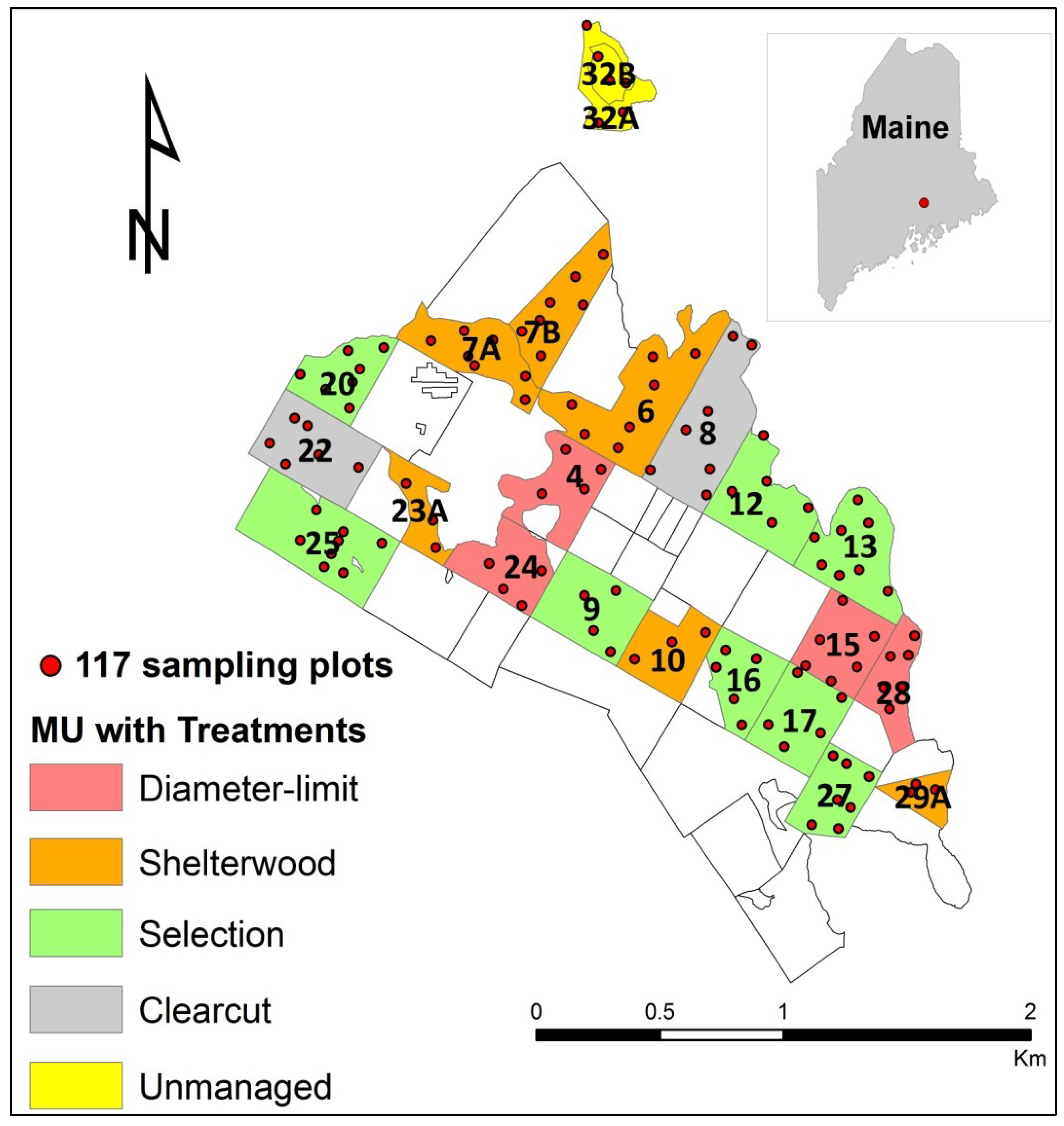
2.1. Study Area

2.2. Inventory Attributes Data

| MU | Area (ha) | Treatment year | Inventory year | Plot (n) | Description of silvicultural treatment | Treatment group |
|---|---|---|---|---|---|---|
| 4 | 10.1 | 1994 | 2009 | 4 | Fixed diameter-limit cutting. Thresholds are 14.0 cm for balsam fir, 24.1 cm for spruce and hemlock, 26.7 cm for white pine, 19.1 cm for cedar and paper birch and 14.0 cm for other hardwoods. | Diameter-limit (DL) |
| 15 | 10.3 | 2001 | 2007 | 6 | ||
| 24 | 9.4 | 1996 | 2005 | 4 | Modified diameter-limit cutting. The third modified diameter-limit cut was applied in 1995. Portions of the stand are in the stem exclusion and understory reinitiation stages of development. | |
| 28 | 7.3 | 1997 | 2007 | 6 | ||
| 9 | 12.2 | 2003 | 2003 | 4 | Five-year cutting cycle. The structural goal is to retain 24.1 m2 ha−1 (trees >11.4 cm). | Selection (SEL) |
| 16 | 8.6 | 2006 | 2006 | 5 | ||
| 12 | 12.5 | 1994 | 2004 | 5 | Ten-year cutting cycle. The structural goal is to retain 20.7 m2 ha−1 (trees >11.4 cm). | |
| 20 | 8.8 | 1998 | 2008 | 7 | ||
| 17 | 10.9 | 1994 | 2005 | 5 | Twenty-year cutting cycle. The structural goal is to retain 16.1 m2 ha−1 (trees > 11.4 cm). | |
| 27 | 8.4 | 1997 | 2007 | 7 | ||
| 13 | 13.2 | 1995 | 2009 | 8 | Crop tree selection. | |
| 25 | 18 | 2009 | 2009 | 8 | ||
| 7A | 10.6 | 1979 | 2003 | 7 | Two-stage uniform shelterwood. Overstory was removed in two harvests; unmerchantable trees >5.08 cm in DBH felled after final overstory removal. | Shelterwood (SHW) |
| 7B | 10.9 | 1979 | 2003 | 7 | ||
| 23A | 5.3 | 2007 | 2007 | 3 | Three-stage uniform shelterwood with PCT . Manual PCT to a residual spacing of 2 × 3 m was applied in 1983. The canopy is not closed, and volunteer growth has occurred between crop trees. | |
| 29A | 3.6 | 2009 | 2010 | 3 | ||
| 6 | 19.6 | 1995 | 2010 | 7 | Multi-stage shelterwood with retention. The overstory will be removed in a series of harvests at 10-year intervals, approximately 2 overstory trees acre−1 will be retained through the next rotation. | |
| 10 | 9.2 | 1995 | 2010 | 3 | ||
| 8 | 17.6 | 1983 | 2008 | 7 | Unregulated harvest/commercial clearcutting. This compartment was initially cut with unregulated (“loggers choice”) harvests. The second harvest was a commercial clearcut in 1982. The stands are in the stand initiation and stem exclusion phases of development. | Clearcut (CC) |
| 22 | 13.6 | 1988 | 2004 | 6 | ||
| 32A | 5.2 | – | 2009 | 3 | Unmanaged natural area (partial cutting had been practiced prior to 1900). | Unmanaged (NAT) |
| 32B | 2.9 | – | 2009 | 3 |
| MU | Max. tree height (m) | Stem density (Trees ha−1) | QMD (cm) | Basal area (m2 ha−1) | Stem volume (m3 ha−1) | Proportion of softwood basal area | ||||||
|---|---|---|---|---|---|---|---|---|---|---|---|---|
| mean | SD | mean | SD | mean | SD | mean | SD | mean | SD | mean | SD | |
| 4 | 11.51 | 2.46 | 7,964 | 4,284 | 6.63 | 1.14 | 24.64 | 6.92 | 82.15 | 25.66 | 0.66 | 0.05 |
| 15 | 11.02 | 2.67 | 6,694 | 4,601 | 6.92 | 1.32 | 21.16 | 7.57 | 56.74 | 17.37 | 0.81 | 0.04 |
| 6 | 12.70 | 4.18 | 12,167 | 5,224 | 5.92 | 1.69 | 28.91 | 5.03 | 110.63 | 69.06 | 0.86 | 0.05 |
| 10 | 15.20 | 3.94 | 7,966 | 4,054 | 7.32 | 1.49 | 29.96 | 3.59 | 139.95 | 46.14 | 0.76 | 0.05 |
| 7A | 10.87 | 1.64 | 467 | 271 | 17.97 | 0.61 | 11.56 | 6.23 | 88.10 | 49.54 | 0.95 | 0.06 |
| 7B | 10.67 | 1.79 | 321 | 118 | 17.40 | 0.71 | 7.63 | 2.79 | 57.02 | 19.91 | 0.84 | 0.06 |
| 8 | 11.14 | 2.17 | 8,507 | 3,170 | 6.96 | 0.96 | 30.43 | 4.40 | 58.63 | 31.30 | 0.56 | 0.04 |
| 22 | 10.10 | 2.32 | 8,277 | 2,892 | 6.27 | 0.89 | 24.15 | 4.09 | 32.02 | 22.81 | 0.51 | 0.03 |
| 9 | 15.62 | 4.25 | 3,948 | 2,223 | 11.19 | 3.24 | 31.67 | 5.85 | 288.53 | 44.46 | 0.91 | 0.06 |
| 16 | 15.10 | 3.79 | 2,281 | 1,691 | 14.95 | 5.62 | 28.56 | 5.52 | 253.21 | 55.88 | 0.84 | 0.05 |
| 12 | 15.00 | 3.73 | 11,240 | 5,177 | 8.98 | 1.96 | 63.02 | 2.82 | 248.56 | 27.05 | 0.80 | 0.07 |
| 20 | 14.13 | 4.39 | 15,533 | 10,945 | 7.76 | 1.92 | 59.46 | 7.81 | 169.17 | 91.60 | 0.71 | 0.07 |
| 13 | 12.43 | 4.35 | 12,668 | 4,663 | 7.83 | 1.74 | 55.23 | 10.01 | 133.98 | 39.81 | 0.84 | 0.07 |
| 25 | 13.49 | 4.15 | 3,894 | 1,824 | 8.66 | 2.97 | 18.61 | 4.95 | 162.36 | 33.66 | 0.69 | 0.05 |
| 17 | 15.73 | 4.33 | 7,668 | 4,549 | 8.22 | 3.15 | 30.19 | 6.38 | 195.10 | 62.79 | 0.87 | 0.06 |
| 27 | 13.56 | 4.13 | 12,126 | 3,450 | 6.48 | 1.03 | 37.94 | 4.68 | 144.66 | 49.83 | 0.79 | 0.05 |
| 24 | 15.20 | 3.94 | 3,665 | 1,953 | 11.21 | 2.16 | 32.36 | 3.99 | 249.83 | 76.84 | 0.83 | 0.04 |
| 28 | 14.33 | 3.90 | 4,708 | 2,431 | 10.45 | 3.67 | 32.64 | 4.54 | 206.60 | 64.12 | 0.77 | 0.04 |
| 23A | 12.94 | 2.51 | 6,971 | 2,222 | 8.50 | 1.38 | 37.65 | 2.05 | 344.73 | 81.62 | 0.76 | 0.03 |
| 29A | 10.60 | 1.34 | 1,915 | 1,811 | 10.92 | 1.69 | 15.29 | 10.12 | 353.03 | 84.37 | 0.98 | 0.02 |
| 32A | 16.25 | 5.10 | 8,479 | 2,588 | 7.58 | 1.47 | 36.78 | 7.94 | 235.11 | 96.55 | 0.63 | 0.02 |
| 32B | 21.48 | 6.24 | 864 | 267 | 28.07 | 5.02 | 50.83 | 7.83 | 662.45 | 88.81 | 0.90 | 0.01 |
| Overall | 13.59 | 3.51 | 6,742 | 3,200 | 10.28 | 2.08 | 32.21 | 5.69 | 194.21 | 53.60 | 0.78 | 0.05 |
2.3. LiDAR System Specifications
2.4. LiDAR Data Processing and Model Calibration Predictions

3. Results
| Attributes | Key variables (mean square error) | R2 (Adj R2) | MB (SD) | RMSE |
|---|---|---|---|---|
| Maximum tree height (m) | Maximum height | 0.869 (0.867) | 1.89 (± 2.06) | 2.80 |
| Stem density (trees ha−1) | Fifth percentile height (3.302), Height kurtosis (5.982), Height L-skewness (6.198) | 0.287 (0.280) | 9 (± 5013) | 4993 |
| QMD (cm) | Percent of the first return above mean (6.5909) Percent of the first return above 1 m (7.8544) Twenty-fifth percentile height (8.3618) | 0.489 (0.434) | −0.05 (± 3.69) | 3.68 |
| Basal area (m2 ha−1) | Percent all returns above 1 m (7.262) Height L-kurtosis (7.564) Ninety-ninth percentile height (7.614) | 0.344 (0.339) | 0.03 (± 13.07) | 13.01 |
| Stem volume (m3 ha−1) | Ninetieth percentile height (7.795) Twentieth percentile height (8.724) Seventy-fifth percentile height (9.757) | 0.721 (0.719) | 1.81 (± 66.96) | 66.70 |
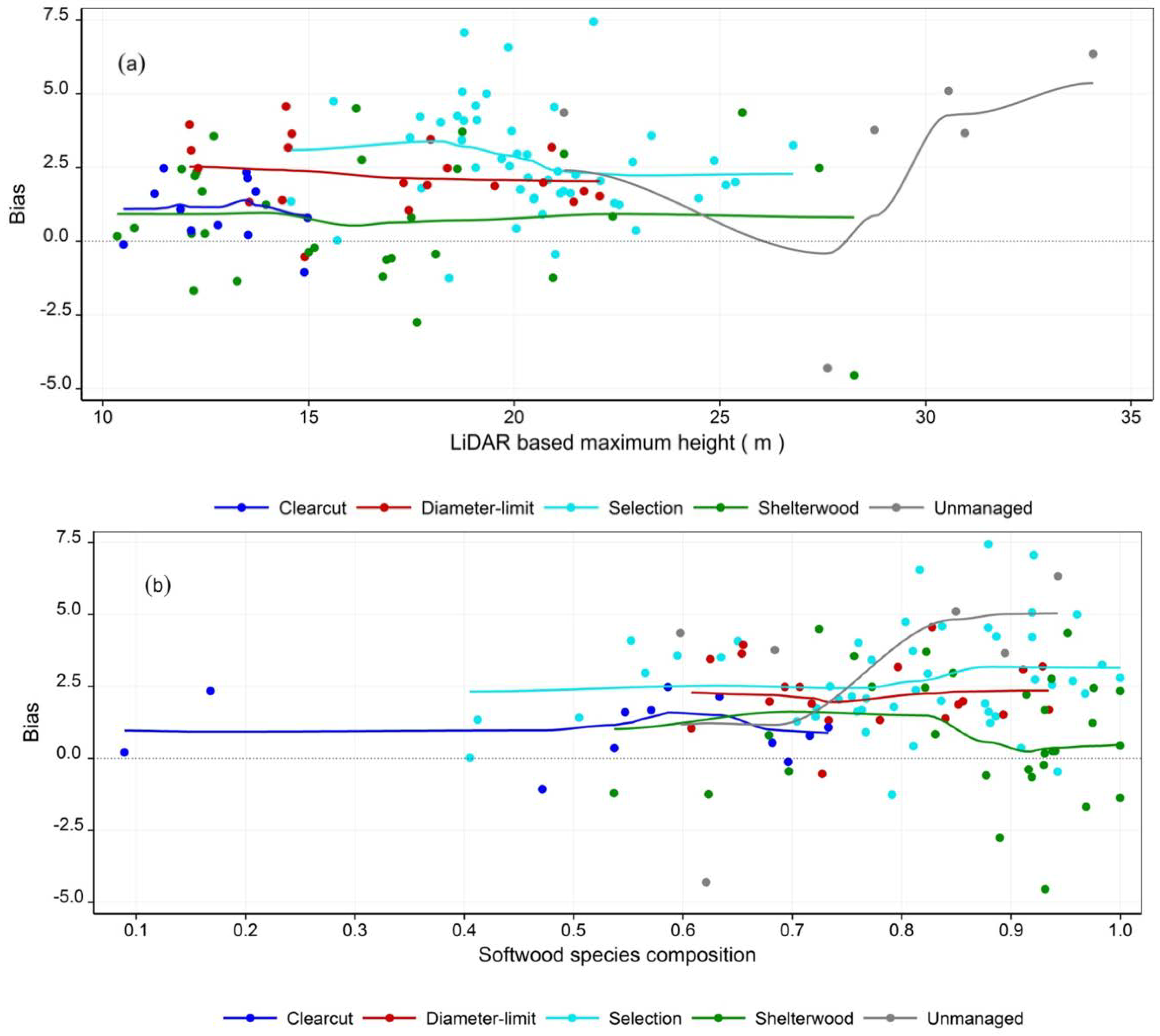
3.1. Maximum Tree Height
| Silvicultural treatments/Species composition | Plot (n) | Max. height MB ± SD (RMSE) (m) | Stem density MB ± SD (RMSE) (trees ha−1) | QMD MB ± SD (RMSE) (cm) | Basal area MB ± SD (RMSE) (m2 ha−1) | Stem volume MB ± SD (RMSE) (m3 ha−1) |
|---|---|---|---|---|---|---|
| Diameter-limit | 20 | 2.27 ± 1.19 (2.55) | −1415 ± 2843 (3111) | 0.05 ± 1.95 (1.90) | −3.63 ± 7.08 (7.80) | −1.12 ± 36.04 (35.14) |
| Selection | 49 | 2.73 ± 1.81 (3.26) | 2119 ± 5755 (6078) | −0.96 ± 3.21 (3.32) | 4.40 ± 15.86 (16.30) | 2.70 ± 40.76 (40.43) |
| Shelterwood | 30 | 0.81 ± 2.15 (2.26) | −2712 ± 4132 (4884) | 1.61 ± 4.51 (4.71) | −7.60 ± 8.88 (11.58) | 5.56 ± 108.05 (106.37) |
| Clearcut | 12 | 1.00 ± 1.08 (1.44) | 1028 ± 3377 (3392) | −1.80 ± 1.36 (2.22) | 5.61 ± 8.24 (9.68) | −26.63 ± 32.46 (40.93) |
| Unmanaged | 6 | 3.15 ± 3.78 (4.67) | −925 ± 3287 (3140) | 2.33 ± 6.48 (6.36) | 3.62 ± 8.38 (8.46) | 42.47 ± 95.22 (96.75) |
| Mixedwood | 31 | 1.59 ± 2.02 (2.55) | −589 ± 4496 (4462) | −0.65 ± 2.89 (2.91) | 0.72 ± 12.02 (11.85) | −12.34 ± 51.53 (52.17) |
| Softwood | 86 | 2.15 ± 2.06 (2.97) | 224 ± 5196 (5171) | 0.17 ± 3.93 (3.91) | −0.22 ± 13.49 (13.41) | 6.91 ± 71.30 (71.22) |
| All plots | 117 | 2.00 ± 2.05 (2.87) | 8.06 ± 5013 (4993) | −0.05 ± 3.69 (3.68) | 0.03 ± 13.07 (13.01) | 1.81 ± 66.96 (66.70) |

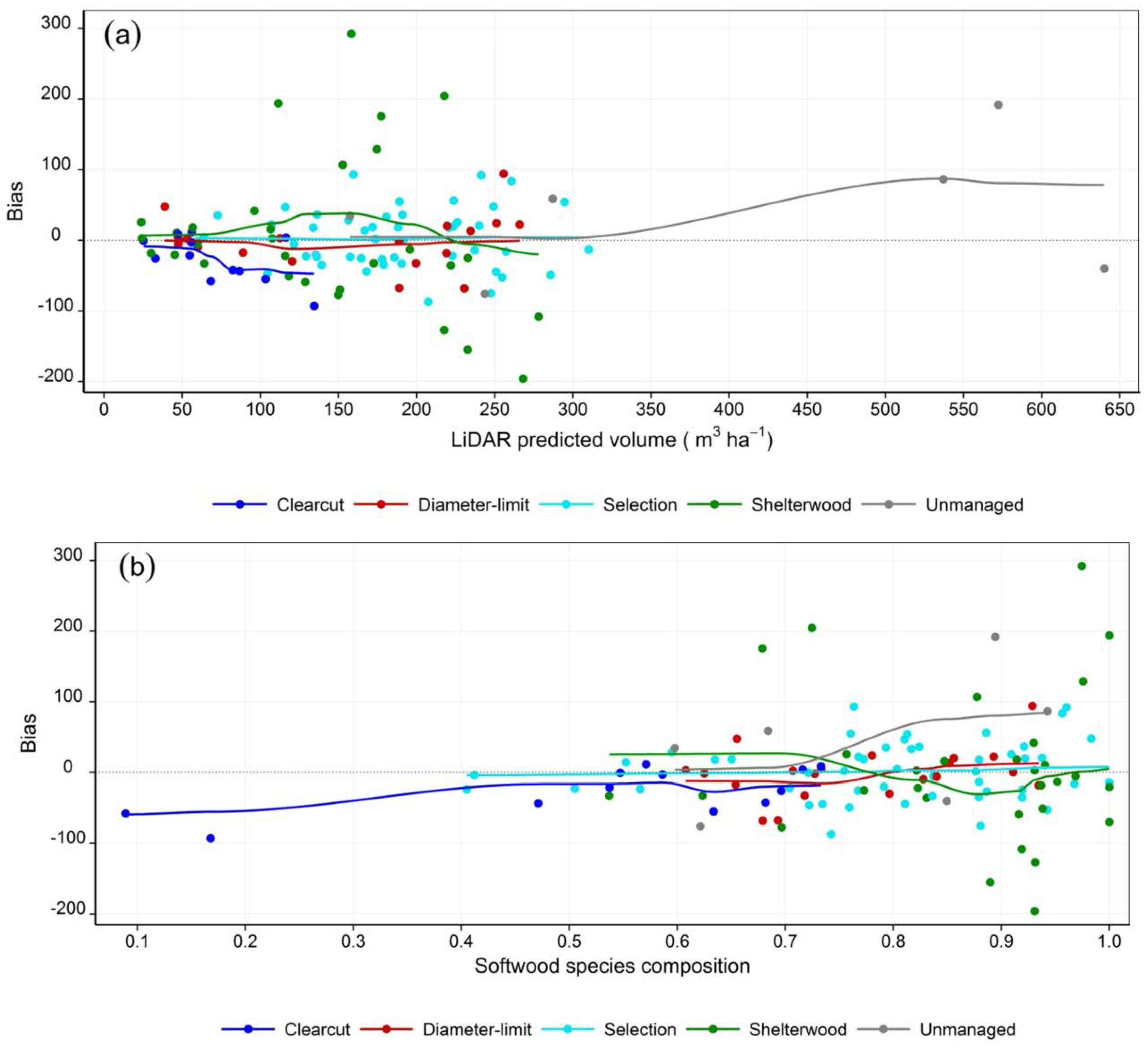
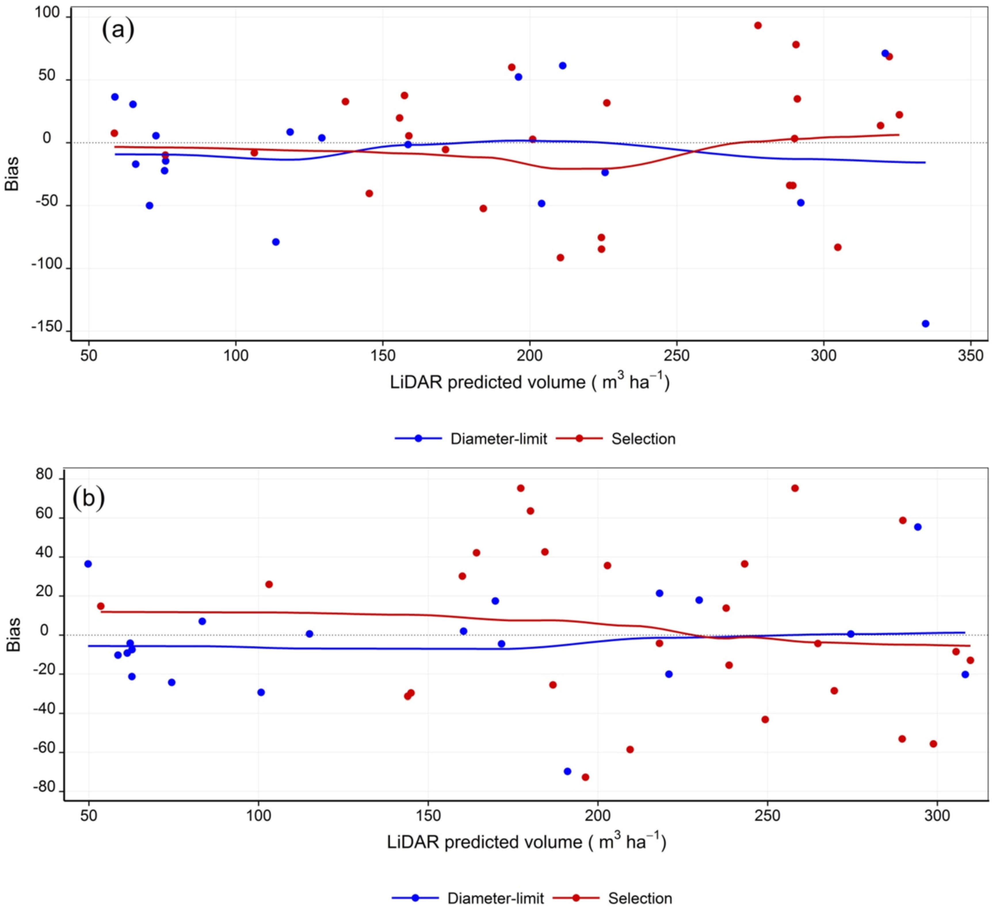
3.2. Stem Volume

| Sampling type | Key variables (mean square error) | R2 (Adj. R2) | MB (SD) (m3 ha−1) | RMSE (m3 ha−1) |
|---|---|---|---|---|
| Research-grade | Mean height (6.777)
Seventy-fifth percentile height (6.784) Fortieth percentile height (6.873) | 0.828 (0.824) | 0.20 (±36.74) | 36.33 |
| Operational-grade | Thirtieth percentile height (6.349)
Twenty-fifth percentile height (6.397) Eightieth percentile height (7.344) | 0.755 (0.749) | −4.21 (±51.22) | 50.81 |

| Silvicultural treatments Species composition | Plot (n) | Stem Volume MB ± SD (RMSE) | |
|---|---|---|---|
| Research-grade (m3 ha−1) | Operational-grade (m3 ha−1) | ||
| Diameter-limit | 18 | −3.09 ± 26.36 (25.88) | −9.90 ± 53.04 (52.49) |
| Selection | 26 | 2.73 ± 43.42 (42.67) | −0.28 ± 50.60 (49.62) |
| Mixedwood | 8 | −3.96 ± 37.80 (35.58) | 13.43 ± 26.10 (27.86) |
| Softwood | 36 | 1.07 ± 36.97 (36.49) | −8.13 ± 54.77 (54.62) |
| All plots | 44 | 0.20 ± 36.74 (36.33) | −4.21 ± 51.22 (50.81) |

4. Discussion
4.1. Predictor Variables in LiDAR Metrics
4.2. Silvicultural Treatments and Species Composition
4.3. Maximum Tree Height
4.4. Stem Volume
5. Conclusions
Acknowledgments
Conflicts of Interest
References
- Stone, C.; Penman, T.; Turner, R. Determining an optimal model for processing lidar data at the plot level: Results for a Pinus radiata plantation in New South Wales, Australia. N. Z. J. For. Sci. 2011, 41, 191–205. [Google Scholar]
- Akay, A.E.; Oğuz, H.; Karas, I.R.; Aruga, K. Using LiDAR technology in forestry activities. Environ. Monit. Assess. 2009, 151, 117–125. [Google Scholar] [CrossRef]
- Hudak, A.T.; Evans, J.S.; Smith, A.M.S. LiDAR utility for natural resource managers. Remote Sens. 2009, 1, 934–951. [Google Scholar] [CrossRef]
- Lefsky, M.A.; Cohen, W.B.; Parker, G.G.; Harding, D.J. Lidar remote sensing for ecosystem studies. BioScience 2002, 52, 19–30. [Google Scholar] [CrossRef]
- Woods, M.; Pitt, D.; Penner, M.; Lim, K.; Nesbitt, D.; Etheridge, D.; Treitz, P. Operational implementation of a LiDAR inventory in boreal Ontario. For. Chron. 2011, 87, 512–528. [Google Scholar]
- Evans, J.; Hudak, A.; Faux, R.; Smith, A.M. Discrete return lidar in natural resources: Recommendations for project planning, data processing, and deliverables. Remote Sens. 2009, 1, 776–794. [Google Scholar] [CrossRef]
- Hummel, S.; Hudak, A.T.; Uebler, E.H.; Falkowski, M.J.; Megown, K.A. A comparison of accuracy and cost of LiDAR vs. stand exam data for landscape management on the Malheur National Forest. J. For. 2011, 109, 267. [Google Scholar]
- Anderson, R.S.; Bolstad, P.V. Estimating aboveground biomass and average annual wood biomass increment with airborne leaf-on and leaf-off LiDAR in Great Lakes forest types. North. J. Appl. For. 2013, 30, 16–22. [Google Scholar] [CrossRef]
- Goerndt, M.E.; Monleon, V.J.; Temesgen, H. Relating forest attributes with area- and tree-based light detection and ranging metrics for western Oregon. West. J. Appl. For. 2010, 25, 105–111. [Google Scholar]
- Næsset, E. Determination of mean tree height of forest stands using airborne laser scanner data. ISPRS J. Photogramm. Remote Sens. 1997, 52, 49–56. [Google Scholar] [CrossRef]
- Clark, M.L.; Clark, D.B.; Roberts, D.A. Small-footprint lidar estimation of sub-canopy elevation and tree height in a tropical rain forest landscape. Remote Sens. Environ. 2004, 91, 68–89. [Google Scholar] [CrossRef]
- Jaskierniak, D.; Lane, P.N.; Robinson, A.; Lucieer, A. Extracting LiDAR indices to characterise multilayered forest structure using mixture distribution functions. Remote Sens. Environ. 2011, 115, 573–585. [Google Scholar]
- García, M.; Riaño, D.; Chuvieco, E.; Danson, F.M. Estimating biomass carbon stocks for a Mediterranean forest in central Spain using LiDAR height and intensity data. Remote Sens. Environ. 2010, 114, 816–830. [Google Scholar] [CrossRef]
- McWilliams, W.H.; Butler, B.J.; Caldwell, L.E.; Griffith, D.M.; Hoppos, M.L.; Laustsen, K.M. The Forests of Maine; U.S. Department of Agriculture, Forest Service, Northeastern Research Station: Newton Square, PA, USA, 2005; p. 188. [Google Scholar]
- Falkowski, M.J.; Smith, A.M.S.; Hudak, A.T.; Gessler, P.E.; Vierling, L.A.; Crookston, N.L. Automated estimation of individual conifer tree height and crown diameter via two-dimensional spatial wavelet analysis of lidar data. Can. J. Remote Sens. 2006, 32, 153–161. [Google Scholar] [CrossRef]
- Popescu, S.C. Estimating biomass of individual pine trees using airborne lidar. Biomass Bioenergy 2007, 31, 646–655. [Google Scholar] [CrossRef]
- Nilsson, M. Estimation of tree heights and stand volume using an airborne lidar system. Remote Sens. Environ. 1996, 56, 1–7. [Google Scholar] [CrossRef]
- Thomas, V.; Treitz, P.; McCaughey, J.H.; Morrison, I. Mapping stand-level forest biophysical variables for a mixedwood boreal forest using lidar: An examination of scanning density. Can. J. For. Res. 2006, 36, 34–47. [Google Scholar] [CrossRef]
- Zimble, D.A.; Evans, D.L.; Carlson, G.C.; Parker, R.C.; Grado, S.C.; Gerard, P.D. Characterizing vertical forest structure using small-footprint airborne LiDAR. Remote Sens. Environ. 2003, 87, 171–182. [Google Scholar] [CrossRef]
- Popescu, S.C.; Wynne, R.H. Seeing the trees in the forest: Using lidar and multispectral data fusion with local filtering and variable window size for estimating tree height. Photogramm. Eng. Remote Sens. 2004, 70, 589–604. [Google Scholar] [CrossRef]
- Hawbaker, T.J.; Gobakken, T.; Lesak, A.; Trømborg, E.; Contrucci, K.; Radeloff, V. Light detection and ranging-based measures of mixed hardwood forest structure. For. Sci. 2010, 56, 313–326. [Google Scholar]
- Means, J.E.; Acker, S.A.; Fitt, B.J.; Renslow, M.; Emerson, L.; Hendrix, C.J. Predicting forest stand characteristics with airborne scanning lidar. Photogramm. Eng. Remote Sens. 2000, 66, 1367–1372. [Google Scholar]
- Jensen, J.L.R.; Williams, C.J.; DeGroot, J.; Humes, K.S.; Conner, T. Estimation of biophysical characteristics for highly variable mixed-conifer stands using small-footprint lidar. Can. J. For. Res. 2006, 36, 1129–1138. [Google Scholar] [CrossRef]
- Næsset, E. Practical large-scale forest stand inventory using a small-footprint airborne scanning laser. Scand. J. For. Res. 2004, 19, 164–179. [Google Scholar] [CrossRef]
- Treitz, P.; Lim, K.; Woods, M.; Pitt, D.; Nesbitt, D.; Etheridge, D. LiDAR sampling density for forest resource inventories in Ontario, Canada. Remote Sens. 2012, 4, 830–848. [Google Scholar] [CrossRef]
- Sendak, P.E.; Brissette, J.C.; Frank, R.M. Silviculture affects composition, growth, and yield in mixed northern conifers: 40-year results from the Penobscot Experimental Forest. Can. J. For. Res. 2003, 33, 2116–2128. [Google Scholar] [CrossRef]
- Li, R.; Weiskittel, A.; Dick, A.R.; Kershaw, J.A.; Seymour, R.S. Regional stem taper equations for eleven conifer species in the Acadian Region of North America: Development and assessment. North. J. Appl. For. 2012, 29, 5–14. [Google Scholar] [CrossRef]
- Weiskittel, A.; Li, R. Development of Regional Taper and Volume Equations: Hardwood Species; University of Maine, School of Forest Resources: Orono, ME, USA, 2012; pp. 87–95. [Google Scholar]
- Weiskittel, A.; Russell, M.; Wagner, R.; Seymour, R. Refinement of the Forest Vegetation Simulator Northeast Variant Growth and Yield Model: Phase III; University of Maine, School of Forest Resources: Orono, ME, USA, 2012; pp. 96–104. [Google Scholar]
- Robinson, A.P.; Wykoff, W.R. Imputing missing height measures using a mixed-effects modeling strategy. Can. J. For. Res. 2004, 34, 2492–2500. [Google Scholar] [CrossRef]
- Heidemann, H.K. Lidar Base Specification Version 1.0: U.S. Geological Survey Techniques and Methods. In Book 11, Collection and Delineation of Spatial Data; US Department of the Interior, US Geological Survey: Sioux Falls, SD, USA, 2012; p. 63. [Google Scholar]
- McGaughey, R.J. FUSION/LDV: Software for LIDAR Data Aalysis and Vsualization, 3.30; USDA Forest Service—Pacific Northwest Research Station: Portland, OR, USA, 2013. [Google Scholar]
- Gonzalez-Ferreiro, E.; Dieguez-Aranda, U.; Barreiro-Fernandez, L.; Bujan, S.; Barbosa, M.; Suarez, J.C.; Bye, I.J.; Miranda, D. A mixed pixel- and region-based approach for using airborne laser scanning data for individual tree crown delineation in Pinus radiata D. Don plantations. Int. J. Remote Sens. 2013, 34, 7671–7690. [Google Scholar] [CrossRef]
- Bolton, D.K.; Coops, N.C.; Wulder, M.A. Measuring forest structure along productivity gradients in the Canadian boreal with small-footprint Lidar. Environ. Monit. Assess. 2013, 185, 6617–6634. [Google Scholar] [CrossRef]
- Hudak, A.T.; Crookston, N.L.; Evans, J.S.; Hall, D.E.; Falkowski, M.J. Nearest neighbor imputation of species-level, plot-scale forest structure attributes from LiDAR data. Remote Sens. Environ. 2008, 112, 2232–2245. [Google Scholar] [CrossRef]
- Li, Y.Z.; Andersen, H.E.; McGaughey, R. A comparison of statistical methods for estimating forest biomass from light detection and ranging data. West. J. Appl. For. 2008, 23, 223–231. [Google Scholar]
- Breiman, L. Random forests. Mach. Learn. 2001, 45, 5–32. [Google Scholar] [CrossRef]
- Liaw, A.; Wiener, M. Classification and regression by randomForest. R News 2002, 2, 18–22. [Google Scholar]
- R Development Core Team. A Language and Environment for Statistical Computing; R Foundation for Statistical Computing: Vienna, Austria, 2013. [Google Scholar]
- Kim, Y.S.; Yang, Z.Q.; Cohen, W.B.; Pflugmacher, D.; Lauver, C.L.; Vankat, J.L. Distinguishing between live and dead standing tree biomass on the North Rim of Grand Canyon National Park, USA using small-footprint lidar data. Remote Sens. Environ. 2009, 113, 2499–2510. [Google Scholar] [CrossRef]
- Parker, R.C.; Glass, P.A. High- vs. low-density LiDAR in a double-sample forest inventory. South. J. Appl. For. 2004, 28, 205–210. [Google Scholar]
- Næsset, E.; Økland, T. Estimating tree height and tree crown properties using airborne scanning laser in a boreal nature reserve. Remote Sens. Environ. 2002, 79, 105–115. [Google Scholar] [CrossRef]
- Su, J.G.; Bork, E.W. Characterization of diverse plant communities in Aspen Parkland rangeland using LiDAR data. Appl. Veg. Sci. 2007, 10, 407–416. [Google Scholar]
- Olson, M.G.; Wagner, R.G. Long-term compositional dynamics of Acadian mixedwood stands under different silvicultural regimes. Can. J. For. Res. 2010, 40, 1993–2002. [Google Scholar] [CrossRef]
- Magnusson, M.; Fransson, J.E.; Holmgren, J. Effects on estimation accuracy of forest variables using different pulse density of laser data. For. Sci. 2007, 53, 619–626. [Google Scholar]
- Magnussen, S.; Boudewyn, P. Derivations of stand heights from airborne laser scanner data with canopy-based quantile estimators. Can. J. For. Res. 1998, 28, 1016–1031. [Google Scholar] [CrossRef]
- Persson, Å.; Holmgren, J.; Söderman, U. Detecting and measuring individual trees using an airborne laser scanner. Photogramm. Eng. Remote Sens. 2002, 68, 925–932. [Google Scholar]
- Van Aardt, J.A.N.; Wynne, R.H.; Oderwald, R.G. Forest volume and biomass estimation using small-footprint lidar-distributional parameters on a per-segment basis. For. Sci. 2006, 52, 636–649. [Google Scholar]
- Gobakken, T.; Næsset, E. Assessing effects of positioning errors and sample plot size on biophysical stand properties derived from airborne laser scanner data. Can. J. For. Res. 2009, 39, 1036–1052. [Google Scholar] [CrossRef]
© 2014 by the authors; licensee MDPI, Basel, Switzerland. This article is an open access article distributed under the terms and conditions of the Creative Commons Attribution license (http://creativecommons.org/licenses/by/3.0/).
Share and Cite
Hayashi, R.; Weiskittel, A.; Sader, S. Assessing the Feasibility of Low-Density LiDAR for Stand Inventory Attribute Predictions in Complex and Managed Forests of Northern Maine, USA. Forests 2014, 5, 363-383. https://0-doi-org.brum.beds.ac.uk/10.3390/f5020363
Hayashi R, Weiskittel A, Sader S. Assessing the Feasibility of Low-Density LiDAR for Stand Inventory Attribute Predictions in Complex and Managed Forests of Northern Maine, USA. Forests. 2014; 5(2):363-383. https://0-doi-org.brum.beds.ac.uk/10.3390/f5020363
Chicago/Turabian StyleHayashi, Rei, Aaron Weiskittel, and Steven Sader. 2014. "Assessing the Feasibility of Low-Density LiDAR for Stand Inventory Attribute Predictions in Complex and Managed Forests of Northern Maine, USA" Forests 5, no. 2: 363-383. https://0-doi-org.brum.beds.ac.uk/10.3390/f5020363