Mapping Above- and Below-Ground Biomass Components in Subtropical Forests Using Small-Footprint LiDAR


Abstract
:
1. Introduction
2. Methods
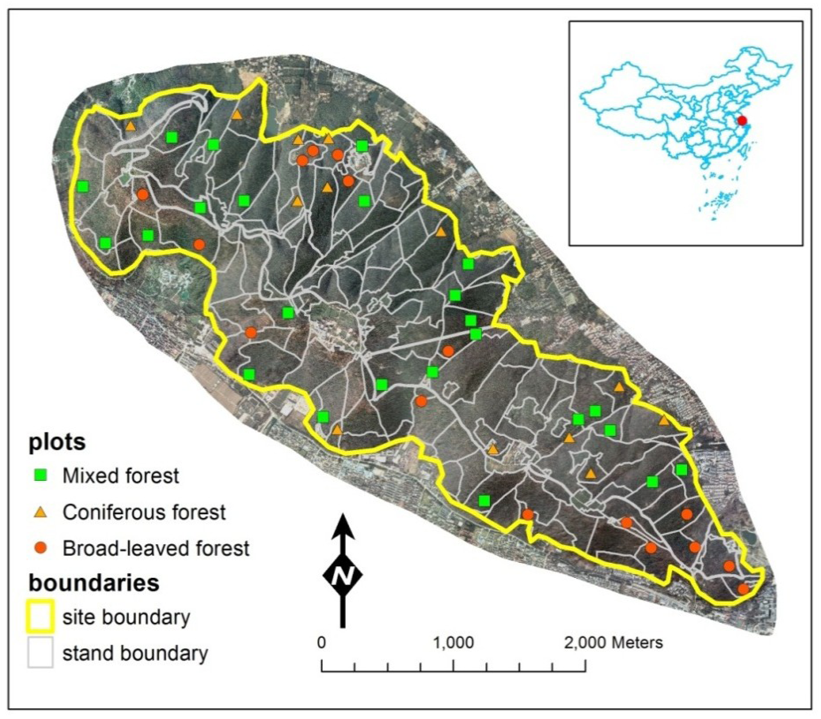
2.1. Study Site and Materials
2.1.1. Study Site

2.1.2. Plot Data

| Variables | Coniferous forest (n = 12) | Broadleaved forest (n = 18) | Mixed forest (n = 23) | |||
|---|---|---|---|---|---|---|
| Range | Mean | Range | Mean | Range | Mean | |
| Biomass-related attributes | ||||||
| HLorey’s | 4.50–14.18 | 10.54 | 7.70–18.52 | 11.96 | 7.79–14.83 | 10.63 |
| DBHavg | 8.15–20.90 | 14.19 | 12.49–22.43 | 15.19 | 10.95–20.62 | 14.22 |
| Wf (foliage) | 1.04–23.57 | 11.69 | 2.13–8.67 | 5.12 | 3.18–19.93 | 7.89 |
| Wb (branch) | 1.62–25.12 | 12.36 | 9.72–44.46 | 19.44 | 6.42–25.33 | 13.90 |
| Ws (trunk) | 8.35–78.70 | 48.48 | 18.65–173.05 | 72.17 | 36.61–100.26 | 67.28 |
| Wa (above-ground) | 11.02–127.39 | 72.52 | 32.03–219.67 | 96.76 | 49.65–141.73 | 89.07 |
| Wr (root) | 6.25–39.42 | 22.60 | 10.31–45.62 | 29.06 | 15.70–43.05 | 27.26 |
| Wt (total) | 17.27–166.81 | 95.12 | 42.34–265.29 | 125.82 | 65.35–184.78 | 116.33 |
| Species composition | ||||||
| Chinese fir (%) | 0–89 | 29 | 0 | 0 | 0–39 | 7 |
| Pines (%) | 0–90 | 53 | 0–29 | 13 | 19–52 | 40 |
| Broadleaved (%) | 2–29 | 18 | 71–100 | 87 | 27–67 | 53 |
2.1.3. Stand Inventory Data
| Variables | Coniferous forest (n = 11) | Broadleaved forest (n = 15) | Mixed forest (n = 19) | |||
|---|---|---|---|---|---|---|
| Range | Mean | Range | Mean | Range | Mean | |
| Biomass-related attributes | ||||||
| Wf (foliage) | 2.69–18.06 | 10.16 | 3.18–12.52 | 8.64 | 4.83–20.76 | 9.61 |
| Wb (branch) | 3.58–18.86 | 12.08 | 8.12–29.57 | 19.48 | 6.08–22.89 | 12.96 |
| Ws (trunk) | 10.34–67.30 | 47.32 | 32.19–135.85 | 78.75 | 34.33–95.01 | 57.40 |
| Wa (above-ground) | 16.56–95.26 | 73.64 | 54.51–183.45 | 108.13 | 50.02–131.73 | 85.29 |
| Wr (root) | 8.31–33.75 | 21.26 | 23.04–39.84 | 29.25 | 13.84–34.97 | 25.16 |
| Wt (total) | 23.81–146.15 | 94.18 | 93.24–216.20 | 140.96 | 75.44–160.28 | 116.37 |
| Species composition | ||||||
| Chinese fir (%) | 0–90 | 21 | 0–10 | 2 | 0–20 | 4 |
| Pines (%) | 0–100 | 61 | 0–30 | 6 | 30–50 | 52 |
| Broadleaved (%) | 0–30 | 19 | 70–100 | 94 | 40–60 | 47 |
2.1.4. LiDAR Data
2.2. LiDAR Metrics
| Metrics | Description |
|---|---|
| Percentile height (h5, h10, h20, …, h95) | The percentiles of the canopy height distributions (5th, 10th, 20th . . . 95th) of first returns. |
| Canopy return density (d0, d1, d2, …, d9) | The canopy return density over a range of relative heights, i.e., percentage (0%–100%) of first returns above the quantiles (0, 10, 20 . . . 90) to total number of first returns. |
| Mean height (hmean) | Mean height above ground of all first returns. |
| Maximum height (hmax) | Maximum height above ground of all first returns. |
| Coefficient of variation of heights (hcv) | Coefficient of variation of heights of all first returns. |
| Canopy cover above 2 meters (CC2m) | Percentages of first returns above 2 m. |
| Canopy cover above mean (CCmean) | Percentages of first returns above the first return mean heights. |
2.3. Statistical Analyses
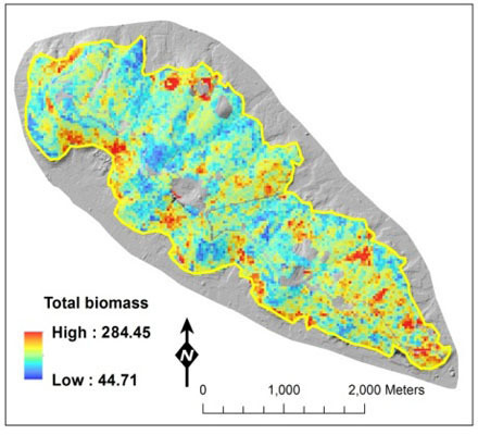
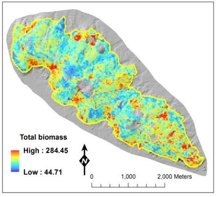
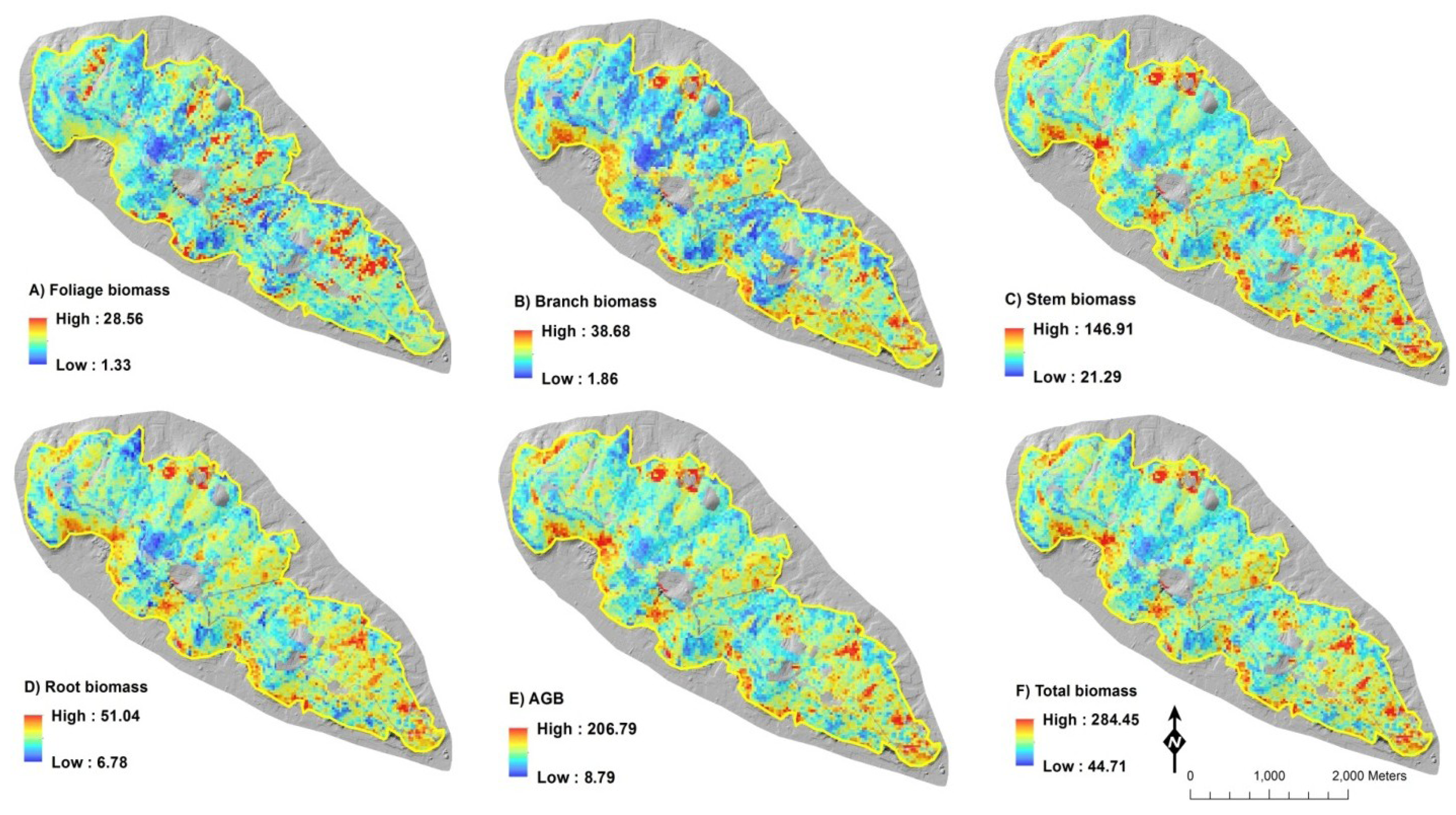
2.4. Biomass Mapping
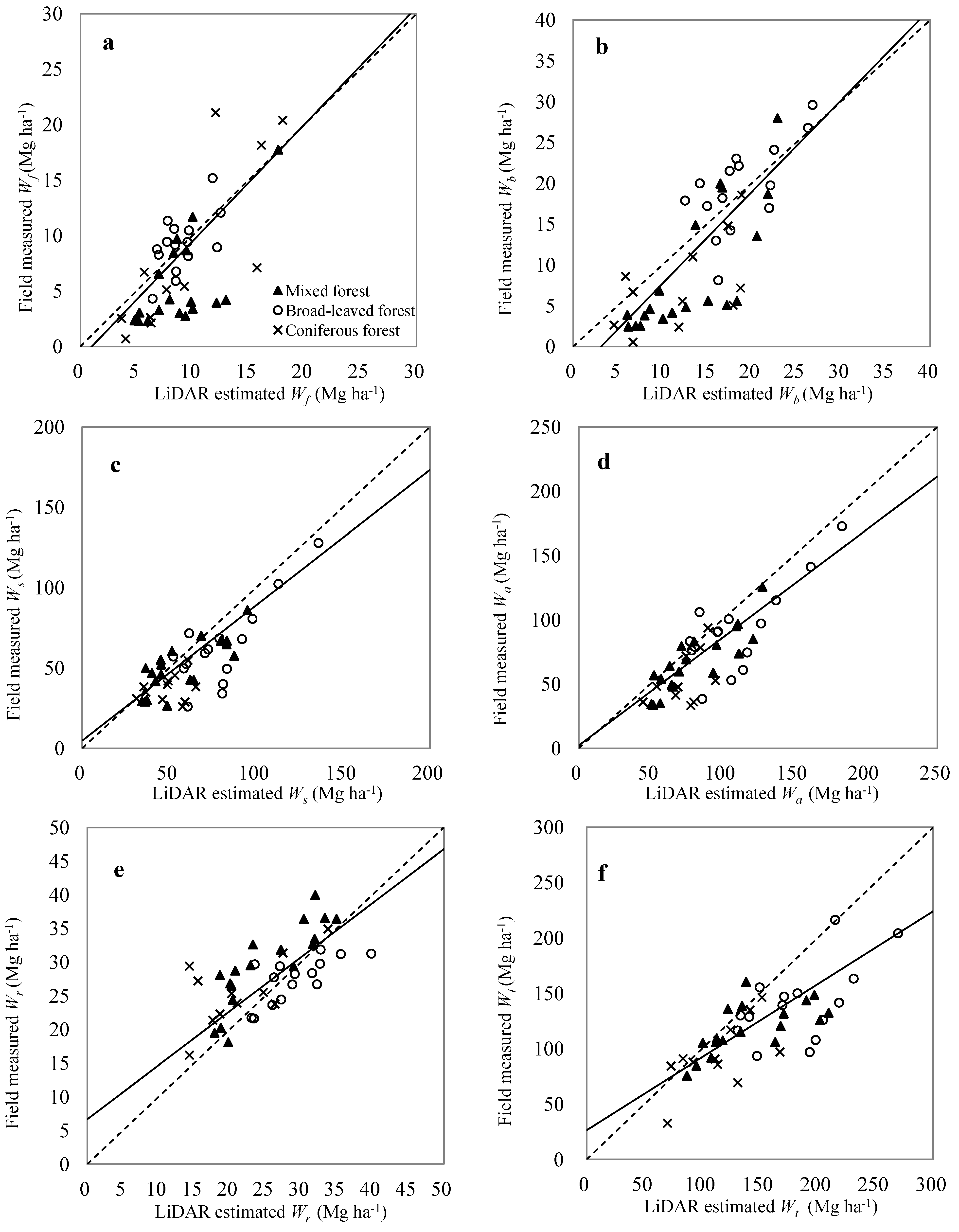
3. Results
| Dependent | Final models | R2 | RMSE | rRMSE (%) |
|---|---|---|---|---|
| Common models | ||||
| Wf | ln Wf = 3.590 + 2.334 ln hcv + 0.867 ln h25 − 3.021 ln CCmean + 2.707 ln d4 | 0.26 | 4.87 | 62.44 |
| Wb | ln Wb = 1.198 − 0.907 ln h10 + 2.635 ln h25 − 0.633 ln CCmean | 0.56 | 4.55 | 29.47 |
| Ws | ln Ws = 2.347 + 1.297 ln h75−2.646 ln CC2m + 2.375 ln d2 | 0.59 | 16.96 | 26.22 |
| Wa | ln Wa = 2.464 − 0.634 ln h10 + 1.997 ln h25 − 0.279 ln CCmean | 0.60 | 20.74 | 23.58 |
| Wr | ln Wr = 1.713 + 0.432 ln hcv + 1.036 ln h25 | 0.59 | 4.85 | 18.10 |
| Wt | ln Wt = 2.803 − 0.625 ln h10 + 1.901 ln h25 − 0.247 ln CCmean | 0.63 | 24.40 | 21.26 |
| Coniferous forest | ||||
| Wf | ln Wf = −1.892 + 1.976 ln hcv + 2.902 ln h25 − 3.059 ln CCmean + 3.055 ln d4 | 0.80 | 4.10 | 35.07 |
| Wb | ln Wb = −3.060 − 0.065 ln h10 + 3.048 ln h25 − 0.136 ln CCmean | 0.81 | 4. 51 | 36.46 |
| Ws | ln Ws = −1.035 + 1.840 ln h75 − 5.718 ln CC2m + 5.961 ln d2 | 0.80 | 10.14 | 20.93 |
| Wa | ln Wa = −0.735 + 0.228 ln h10 + 2.166 ln h25 + 0.076 ln CCmean | 0.83 | 18.52 | 25.54 |
| Wr | ln Wr = 0.086 + 0.421 ln hcv + 1.799 ln h25 | 0.83 | 4.46 | 19.74 |
| Wt | ln Wt = 0.054 + 0.071 ln h10 + 2.136 ln h25 + 0.026 ln CCmean | 0.84 | 22.28 | 23.42 |
| Broadleaved forest | ||||
| Wf | ln Wf = 4.980 + 1.227 ln hcv + 0.327 ln h25 − 4.652 ln CCmean + 3.685 ln d4 | 0.21 | 1.90 | 37.16 |
| Wb | ln Wb = 3.104 + 0.882 ln h10 + 0.173 ln h25 − 0.605 ln CCmean | 0.71 | 4.79 | 24.67 |
| Ws | ln Ws = 6.937 + 1.275 ln h75 − 7.328 ln CC2m + 6.069 ln d2 | 0.77 | 18.04 | 24.99 |
| Wa | ln Wa = 3.407 − 0.336 ln h10 + 1.622 ln h25 − 0.471 ln CCmean | 0.62 | 24.69 | 25.52 |
| Wr | ln Wr = 2.271 + 0.284 ln hcv + 0.689 ln h25 | 0.53 | 4.76 | 16.37 |
| Wt | ln Wt = 3.560 − 0.515 ln h10 + 1.685 ln h25 − 0.382 ln CCmean | 0.64 | 27.70 | 22.02 |
| Mixed forest | ||||
| Wf | lnWf =−1.925 + 2.595 ln hcv + 0.232 ln h25 − 0.643 ln CCmean + 1.037 ln d4 | 0.54 | 3.41 | 43.22 |
| Wb | ln Wb =−1.802 − 1.228 ln h10 + 2.391 ln h25 + 0.398 ln CCmean | 0.62 | 4.25 | 30.60 |
| Ws | ln Ws = 1.336 + 1.491 ln h75 − 2.765 ln CC2m + 2.643 ln d2 | 0.70 | 11.28 | 16.77 |
| Wa | ln Wa = 2.295 − 0.451 ln h10 + 1.588 ln h25 − 0.084 ln CCmean | 0.58 | 17.10 | 19.20 |
| Wr | ln Wr = 1.444 + 0.295 ln hcv + 1.091 ln h25 | 0.64 | 4.27 | 15.66 |
| Wt | ln Wt = 2.481 − 0.428 ln h10 + 1.504 ln h25 − 0.028 ln CCmean | 0.62 | 20.73 | 17.82 |
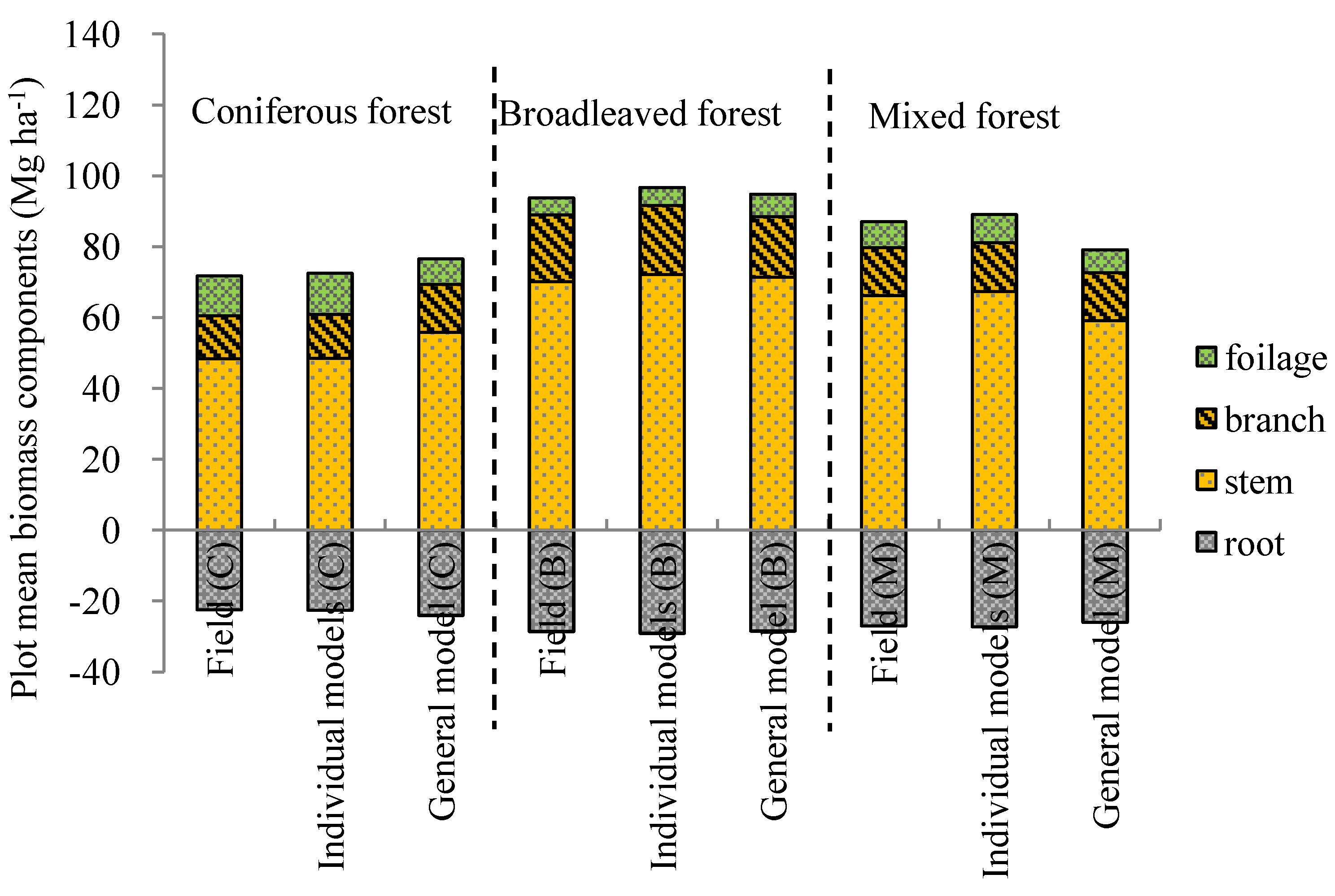
| Variables (Mg ha−1) | Coniferous forest (n = 12) | Broadleaved forest (n = 18) | Mixed forest (n = 23) | ||||||
|---|---|---|---|---|---|---|---|---|---|
| #OM | #MD | #SD | #OM | #MD | #SD | #OM | #MD | #SD | |
| Wf | 11.69 | −1.09 NS | 4.78 (40.9%) | 5.12 | −0.87 NS | 2.34 (45.7%) | 7.89 | 0.48 NS | 1.44 (18.3%) |
| Wb | 12.36 | −0.51 NS | 4.87 (39.4%) | 19.44 | −1.02 NS | 5.87 (30.2%) | 13.90 | −0.21 NS | 3.25 (23.4%) |
| Ws | 48.48 | −1.96 NS | 11.96 (24.7%) | 72.17 | −0.42 NS | 22.43 (31.1%) | 67.28 | −1.02 NS | 10.16 (15.1%) |
| Wa | 75.52 | −0.13 NS | 13.91 (18.4%) | 96.76 | −2.33 NS | 29.15 (30.1%) | 89.07 | −1.76 NS | 11.12 (12.5%) |
| Wr | 22.60 | −0.94 NS | 3.25 (14.4%) | 29.06 | −1.12 NS | 6.50 (22.4%) | 27.26 | −0.04 NS | 3.32 (12.2%) |
| Wt | 95.12 | 0.02 NS | 16.60 (17.5%) | 125.82 | −4.98 NS | 20.76 (16.5%) | 116.33 | −1.07 NS | 24.83 (21.3%) |
| Variables (Mg ha−1) | Coniferous forest (n = 11) | Broadleaved forest (n = 15) | Mixed forest (n = 19) | |||||||
|---|---|---|---|---|---|---|---|---|---|---|
| #OM | #MD | #SD | #OM | #MD | #SD | #OM | #MD | #SD | ||
| Wf | 7.08 | 1.52 NS | 2.63 | 9.25 | −0.24 NS | 2.15 | 6.37 | 1.49 * | 1.88 | |
| (37.1%) | (22.2%) | (29.5%) | ||||||||
| Wb | 7.83 | 3.01 NS | 3.10 | 19.48 | −0.37 NS | 6.18 | 9.57 | 3.05 * | 3.92 | |
| (39.6%) | (31.7%) | (41.0%) | ||||||||
| Ws | 38.93 | 10.54 * | 12.93 | 67.21 | 12.50 ** | 32.85 | 52.32 | 3.02 NS | 10.50 | |
| (33.2%) | (48.9%) | (20.1%) | ||||||||
| Wa | 59.48 | 9.90 NS | 10.43 | 94.12 | 15.81 * | 31.55 | 66.42 | 8.90 ** | 12.32 | |
| (17.5%) | (33.5%) | (18.5%) | ||||||||
| Wr | 24.94 | −2.27 NS | 2.28 | 27.47 | 1.78 NS | 7.43 | 29.49 | −4.33 ** | 3.35 | |
| (11.4%) | ||||||||||
| (9.14%) | (27.0%) | |||||||||
| Wt | 96.63 | 10.14 NS | 15.70 | 141.72 | 15.20 NS | 19.03 | 115.47 | 14.05 * | 25.62 | |
| (16.2%) | (13.4%) | (22.2%) | ||||||||


4. Discussion
5. Conclusions
Acknowledgments
Author Contributions
Conflicts of Interest
References
- Dixon, R.K.; Brown, S.; Houghton, R.A.; Solomon, A.M.; Trexler, M.C.; Wisniewski, J. Carbon Pools and Flux of Global Forest Ecosystems. Science 1994, 263, 185–190. [Google Scholar]
- Pancel, L. Tropical Forestry Handbook; Springer-Verlag: Berlin, Germany, 1993. [Google Scholar]
- Fang, J.; Chen, A. Dynamic Forest Biomass Carbon Pools in China and Their Significance. Acta Bot. Sin. 2001, 43, 967–973. [Google Scholar]
- Wang, X.; Feng, Z.; Ouyang, Z. The Impact of Human Disturbance on Vegetative Carbon Storage in Forest Ecosystems in China. For. Ecol. Manag. 2001, 148, 117–123. [Google Scholar] [CrossRef]
- Lambert, M.C.; Ung, C.H.; Raulier, F. Canadian National Tree Aboveground Biomass Equations. Can. J. For. Res. 2005, 35, 1996–2018. [Google Scholar] [CrossRef]
- Saatchi, S.; Halligan, K.; Despain, D.G.; Crabtree, R.L. Estimation of Forest Fuel Load from Radar Remote Sensing. IEEE Trans. Geosci. Remote Sens. 2007, 45, 1726–1740. [Google Scholar]
- Gibbs, H.K.; Brown, S.; Niles, J.O.; Foley, J.A. Monitoring and Estimating Tropical Forest Carbon Stocks: Making REDD a Reality. Environ. Res. Lett. 2007, 2, 1–13. [Google Scholar]
- Rosenqvist, A.; Shimada, M.; Igarashi, T.; Watanabe, M.; Tadono, T.; Yamamoto, H. Support to Multi-National Environmental Conventions and Terrestrial Carbon Cycle Science by ALOS and ADEOS-II-the Kyoto & Carbon Initiative. In Proceedings of the IGARSS 2003, IEEE International Geoscience and Remote Sensing Symposium, VOLS I-VII, Learning from Earth’s Shapes and Sizes, New York, NY, USA, 21–25 July 2003; pp. 1493–1495.
- Richards, P.W. The Tropical Rain Forest: An Ecological Study; Cambridge University Press: Cambridge, UK, 1996. [Google Scholar]
- Lefsky, M.A.; Cohen, W.B.; Parker, G.G.; Harding, D.J. LiDAR Remote Sensing for Ecosystem Studies. BioScience 2002, 52, 19–30. [Google Scholar] [CrossRef]
- Dubayah, R.; Drake, J. LiDAR Remote Sensing for Forestry. J. For. 2000, 98, 44–46. [Google Scholar]
- Patenaude, G.; Hill, R.A.; Milne, R.; Gaveau, D.L.A.; Briggs, B.B.J.; Dawson, T.P. Quantifying Forest above Ground Carbon Content Using LiDAR Remote Sensing. Remote Sens. Environ. 2004, 93, 368–380. [Google Scholar] [CrossRef]
- Lim, K.; Treitz, P.; Baldwin, K.; Morrison, I.; Green, J. LiDAR Remote Sensing of Biophysical Properties of Tolerant Northern Hardwood Forests. Can. J. Remote Sens. 2003, 29, 658–678. [Google Scholar] [CrossRef]
- Naesset, E.; Gobakken, T. Estimation of above- and below-Ground Biomass Across Regions of the Boreal Forest Zone Using Airborne Laser. Remote Sens. Environ. 2008, 112, 3079–3090. [Google Scholar] [CrossRef]
- Huang, W.L.; Sun, G.Q.; Dubayah, R.; Cook, B.; Montesano, P.; Ni, W.J.; Zhang, Z.Y. Mapping Biomass Change after Forest Disturbance: Applying LiDAR Footprint-Derived Models at Key Map Scales. Remote Sens. Environ. 2013, 134, 319–332. [Google Scholar]
- Drake, J.B.; Knox, R.G.; Dubayah, R.O.; Clark, D.B.; Condit, R.; Blair, J.B.; Hofton, M. Above-Ground Biomass Estimation in Closed Canopy Neotropical Forests Using LiDAR Remote Sensing: Factors Affecting the Generality of Relationships. Glob. Ecol. Biogeogr. 2003, 12, 147–159. [Google Scholar]
- Saatchi, S.S.; Harris, N.L.; Brown, S.; Lefsky, M.; Mitchard, E.T.A.; Salas, W.; Zutta, B.R.; Buermann, W.; Lewis, S.L.; Hagen, S.; Petrova, S.; White, L.; Silman, M.; Morel, A. Benchmark Map of Forest Carbon Stocks in Tropical Regions across Three Continents. In Proceedings of the National Academy of Sciences of the United States of America, Irvine, CA, USA, December 2011. [CrossRef]
- Tsui, O.W.; Coops, N.C.; Wulder, M.A.; Marshall, P.L.; McCardle, A. Using Multi-Frequency Radar and Discrete-Return LiDAR Measurements to Estimate Above-Ground Biomass and Biomass Components in a Coastal Temperate Forest. ISPRS J. Photogr. Remote Sens. 2012, 69, 121–133. [Google Scholar] [CrossRef]
- Næsset, E. Estimation of Above- and Below-Ground Biomass in Boreal Forest Ecosystems. In Laser-Scanners for Forest and Landscape Assessment; ISPRS Archives; Thies, M., Koch, B., Spiecker, H., Weinacker, H., Eds.; International Society for Photogrammetry and Remote Sensing: Freiburg, Germany, 2004; pp. 145–148. [Google Scholar]
- Pan, B.H.; Zhang, Z.M.; Cao, T.R. Natural Vegetation of Yusan National Forest Park in Jiangsu Province, China. J. Cent. South. Univ. For. Technol. 2007, 27, 123–128. [Google Scholar]
- Bastide, F.; Alexander, K. Satellite-Based Augmentation Systems (SBAS) Combined Performance. In Presented at International Committee on GNSS (ICG-4), Working Group A, St. Petersburg, Russia, 14–18 September 2009.
- Feng, Z.W.; Wang, X.K.; Wu, G. Biomass and Productivity of Chinese Forest Ecosystem; Science Press: Beijing, China, 1999. [Google Scholar]
- Anonymous. RIEGL Software Manual: RiANALYZE for RIEGL Airborne Laser Scanners LMS-Q680, 5th ed.; RIEGL: Horn, Austria, 2008. [Google Scholar]
- Naesset, E. Predicting Forest Stand Characteristics with Airborne Scanning Laser Using a Practical Two-Stage Procedure and Field Data. Remote Sens. Environ. 2002, 80, 88–99. [Google Scholar] [CrossRef]
- Naesset, E. Effects of Different Flying Altitudes on Biophysical Stand Properties Estimated from Canopy Height and Density Measured with a Small-Footprint Airborne Scanning Laser. Remote Sens. Environ. 2004, 91, 243–255. [Google Scholar] [CrossRef]
- Ferster, C.J.; Coops, N.C.; Trofymow, J.A. Aboveground Large Tree Mass Estimation in a Coastal Forest in British Columbia Using Plot-Level Metrics and Individual Tree Detection from LiDAR. Can. J. Remote Sens. 2009, 35, 270–275. [Google Scholar] [CrossRef]
- Kim, Y.; Yang, Z.Q.; Cohen, W.B.; Pflugmacher, D.; Lauver, C.L.; Vankat, J.L. Distinguishing between Live and Dead Standing Tree Biomass on the North Rim of Grand Canyon National Park, USA Using Small-Footprint LiDAR Data. Remote Sens. Environ. 2009, 113, 2499–2510. [Google Scholar] [CrossRef]
- Kraus, K.; Pfeifer, N. Determination of Terrain Models in Wooded Areas with Airborne Laser Scanner Data. ISPRS J. Photogr. Remote Sens. 1998, 53, 193–203. [Google Scholar] [CrossRef]
- Naesset, E.; Bjerknes, K.O. Estimating Tree Heights and Number of Stems in Young Forest Stands Using Airborne Laser Scanner Data. Remote Sens. Environ. 2001, 78, 328–340. [Google Scholar] [CrossRef]
- Sprugel, D.G. Correcting for Bias in Log-Transformed Allometric Equations. Ecology 1983, 64, 209–210. [Google Scholar] [CrossRef]
- Weisberg, S. Applied Linear Regression, 2nd ed.; Wiley: New York, NY, USA, 1985. [Google Scholar]
- Kutner, M.; Nachtsheim, C.; Neter, J.; Li, W. Applied Linear Statistical Models, 5th ed.; McGraw-Hill/Irwin: New York, NY, USA, 2004. [Google Scholar]
- Fu, T.; Pang, Y.; Huang, Q.F.; Liu, Q.W.; Xu, G.C. Prediction of Subtropical Forest Parameters Using Airborne Laser Scanner. J. Remote Sens. 2011, 15, 1092–1104. [Google Scholar]
- Pang, Y.; Li, Z.Y. Inversion of Biomass Components of the Temperate Forest Using Airborne LiDAR Technology in Xiaoxing’ an Mountains, Northeastern of China. Chin. J. Plant Ecol. 2012, 36, 1095–1105. [Google Scholar] [CrossRef]
© 2014 by the authors; licensee MDPI, Basel, Switzerland. This article is an open access article distributed under the terms and conditions of the Creative Commons Attribution license (http://creativecommons.org/licenses/by/3.0/).
Share and Cite
Cao, L.; Coops, N.C.; Innes, J.; Dai, J.; She, G. Mapping Above- and Below-Ground Biomass Components in Subtropical Forests Using Small-Footprint LiDAR. Forests 2014, 5, 1356-1373. https://0-doi-org.brum.beds.ac.uk/10.3390/f5061356
Cao L, Coops NC, Innes J, Dai J, She G. Mapping Above- and Below-Ground Biomass Components in Subtropical Forests Using Small-Footprint LiDAR. Forests. 2014; 5(6):1356-1373. https://0-doi-org.brum.beds.ac.uk/10.3390/f5061356
Chicago/Turabian StyleCao, Lin, Nicholas C. Coops, John Innes, Jinsong Dai, and Guanghui She. 2014. "Mapping Above- and Below-Ground Biomass Components in Subtropical Forests Using Small-Footprint LiDAR" Forests 5, no. 6: 1356-1373. https://0-doi-org.brum.beds.ac.uk/10.3390/f5061356