An Integer Programming Model to Determine Land Use Trajectories for Optimizing Regionally Integrated Ecosystem Services Delivery

Abstract

BIOLP is an Integer Programming model based on the Balanced Compromise Programming multi-criteria decision method. The aim of BIOLP is to determine how a set of land use types should be distributed over space and time in order to optimize the multi-dimensional land performance of a region. Trajectories were defined as the succession of specific land use types over 30 years, assuming that land use changes can only occur at fixed intervals of 10 years. A database that represents the Tabacay catchment (Ecuador) as a set of land units with associated performance values was used as the input for BIOLP, which was then executed to determine the trajectories distribution that optimizes regional performance. The sensitivity of BIOLP to uncertainty in the input data, simulated through random variations on the performance values, was also tested. BIOLP showed a relative stability on its results under these conditions of stochastic, restricted changes. Additionally, the behaviour of BIOLP under different settings of its balancing and relative importance parameters was studied. Stronger variations on the outcomes were observed in this case, which indicate the influential role that such parameters play. Finally, the inclusion of performance thresholds in BIOLP was tested through the addition of sample constraints that required some of the criteria at stake to exceed predefined values. The outcome of the optimization exercises makes clear that the phenomenon of trade off between the provisioning service of the land (income) and the regulation and maintenance services (runoff, sediment, SOC) is crucial. BIOLP succeeds in accounting for this complex multi-dimensional phenomenon when determining the optimal spatio-temporal distributions of land use types. Despite this complexity, it is confirmed that the weights attributed to the provisioning or to the regulation and maintenance services are the main determinants for having the land use distributions dominated by either agriculture or forest.

1. Introduction

Land use planning is an essential tool for achieving the ultimate goal of sustainable territorial development ([1]). Land use planning requires making decisions that involve multiple environmental and socio-economic criteria ([2]). Such decisions are typically based on two approaches. On the one hand, they are related to the suitability of a land unit (portion of land with uniform characteristics ([3,4])) for establishing a particular land use type (LUT); and, on the other hand, they are targeted at determining the LUT that would optimize the performance of a specific land unit. The former is an instance of a site location problem: Where should a given LUT be established?, while the latter corresponds to solving a What? question: What LUT should be applied to a given area? Due to the fact that land units are not isolated entities, but interacting components of a larger system, i.e., the region of interest, independent land performance assessment of separate land units is of limited usefulness. Instead, enhancing regional performance, expressed as the integral contribution of all individual land units, is typically the goal of most land use planning projects.

The utility of land use planning becomes apparent when considering its goals and consequences in the long term, i.e., the objectives of land use planning cannot be confined to the immediate future. This is particularly true when land use planning involves LUT like forests, which produce gradual effects on the environment. In such cases the incorporation of the temporal dimension in the problem becomes a requirement. This leads to a more elaborated version of the What? question, in the sense that land use management of a region over a medium or long term will most certainly require the definition of LUT sequences that should be applied within a time span in order to enhance regional land performance. The temporal dimension in this context can be considered in two ways: absolute, when land performance is assessed with reference to a concrete period in time, e.g., the period 2015–2045; and relative, when land performance is not linked to any specific point in time, i.e., land performance in this case is assessed for a reference, abstract, period of time. Considering time in the absolute way can be claimed to be more realistic but it is also more complex, since in that case the expected land performance corresponding to a specific point in time must be determined. To compute this performance, the existing conditions at that particular point in time should be determined and involved in the estimations. Not linking the study period to any specific point in time offers a more abstract picture of reduced complexity.

In [5] a Mathematical Programming model was introduced and applied to determine the land use configuration that would optimize regional land performance aggregated over a 30 years period without considering land use trajectories. This model was formulated using the Balanced Compromise Programming Multi-Criteria Decision Method (MCDM). The latter is a variant of the well-known Compromise Programming MCDM ([6]). The term “land use configuration” is used in [5] to refer to a specific distribution of a predefined number of LUT over the study region with a view to fulfil multiple criteria. Besides introducing and applying this model, [5] reports on the comparison of its output with respect to other multi-criteria decision making methods.

In the present study we build further upon [5] to address the optimization of the land performance of a region considering the sequential implementation of four possible LUT: crops, pasture, pine plantation and eucalypt plantation. The Mathematical Programming model introduced in [5], was used to determine the way in which these LUT should be sequenced over the land units in the study area and over a time span of 30 years, with the aim of achieving an optimal cumulative regional performance. Like in [5], land performance was expressed as the trade-off of five continuous and conflicting attributes: runoff production, sediment production, organic carbon stock in soil, organic carbon stock in biomass, and monetary income. These performance attributes are considered ecological indicators of different ecosystem services (ESS). Given that the study region is represented as a set of land units, the output of this model is a configuration in which each land unit is assigned a LUT sequence, or trajectory. In the temporal dimension, 10 year intervals covering a time span of 30 years are considered. In addition to test the performance of this model for the data initially available and with a set of fixed parameter values, in this paper we also assess the behaviour of the model under conditions of uncertainty in the input data and evaluate its sensitivity to varying parameter values. Moreover, the way in which the results are affected when including performance thresholds as additional constraints was investigated.

2. Literature Review

Land use planning and management, both in urban and rural areas, can be tackled using a multitude of different approaches. Such approaches are typically members of one of two broad families of methods: (i) exact techniques (e.g., mathematical programming models); or (ii) (meta-)heuristic methods. Principles taken from these two areas have been applied to allocate different uses to specific area units within a region. In this context, these techniques must take into account the fact that land use planners are typically interested in several criteria of different nature. Furthermore, some degree of conflict is commonly observed among these criteria, in the sense that enhancing one of them decreases the level of one or more of the others. In such cases, the application of MCDMs ([7,8]) becomes a necessity. These methods are well suited to find near to optimal solutions while trading off the conflicting criteria at stake. They also typically allow to express differences on the relative importance of these criteria.

Besides the method introduced in [5], which is further elaborated in the present article, several other examples of multi-criteria mathematical programming models exist. For instance, [9] introduces a dynamic mathematical programming model that is capable of suggesting optimal land use plans. This model considers several environmental (carbon emissions in particular and environmental pollution in general) as well as socio-economic criteria (economic development and employment opportunities). It also integrates the decision maker preferences in the form of a so-called compromise index. Another example of an application of a MCDM for land use planning is [10], which describes the application of the Ordered Weighted Averaging multi-criteria evaluation method in order to assess the safety of sites based on several criteria like earthquake risk and site type. The latter is an example of an exact method that does not pertain to mathematical programming. [11] applies the Goal Programming MCDM ([12]) to optimize the environmental performance of agriculture. This application starts by defining a system of “high environmental state” as the goal at which the current environmental state is aimed. This model generates land use plans based on the optimization of three environmental criteria: nitrogen in water, sediment in water and water yield. Additionally, [13] compares the performance of an Integer Programming model and a heuristic technique when locating areas within a river catchment that should be afforested in order to minimize sediment yield.

Besides [13], several other examples of heuristic and meta-heuristic methods can be cited. For instance, [14] introduces a method based on a genetic algorithm to determine land use plans that optimize socio-economic, environmental, and even topological (compactness) criteria. Another example of an application of a genetic algorithm in land use planning is reported in [15], which describes a genetic-algorithm-based software library that can be applied to optimize land use configurations. It uses a patch topology representation to stratify the study region represented as a raster into areas of contiguous cells. Each of these areas, or patches, is considered as an individual entity, to which a specific land use type can be assigned. Another novel representation of geographical entities is introduced in [16], which describes the use of graps to represent a geographical region. This representation is then used as the input for evolutionary algorithms, the general class of which genetic algorithms are instances, to solve geographical optimization problems, like area selection or region partitioning. [17] uses the principles of simulated annealing in order to develop a method for determining optimal land allocation patterns that fulfil multiple objectives.

Mathematical programming and (meta-)heuristics are not mutually exclusive. Techniques that combine principles from both areas have also been reported in the literature. An example is [18], which formulates a Goal Programming model to solve a multi-site land use allocation problem. This type of problems consists in assigning more than one land use type to a given area. Since the resulting Goal Programming model is non-linear, meta-heuristics are applied to solve the problem in a reasonable time. In particular, the performance of a genetic algorithm is contrasted to that of a simulated annealing approach. Topological factors like compactness and contiguity are considered among the optimization criteria.

Several studies about sensitivity analyses of multi-criteria land use planning methods and their behaviour under data uncertainty have been conducted in the past and reported in the literature. For instance, [19] describes the analysis of the sensitivity of MCDMs in the context of a Geographic Information System to variations on the relative importance values of each criterion. The simulations performed in [19] also allowed to determine the criteria that were particularly sensitive to such variations. In [20] a method for determining the suitability of sites for conversion to perennial bioenergy crops is introduced. A simulation approach was applied to evaluate the influence of uncertainty of the input data and parameters on the model behaviour and outcomes. A closely related study is reported in [21], which introduces a model that integrates simulation, and analysis and visualization of uncertainty in the context of spatial decision support. The presented tool includes a spatio-temporal modelling framework, which simulates land use changes dynamically over several time steps. It also incorporates a Monte Carlo analysis framework that, based on the simulation component, is capable of producing stochastic maps. An assessment of the impact that uncertainty in both the input variables and the parameter settings have on the outcomes of this model is discussed.

3. Materials and Methods

3.1. Study Region

The study region is the hydrographical catchment of the Tabacay river, located in the province of Cañar, in the southern Andes of the republic of Ecuador. The area of the Tabacay catchment is 66.5 km² and its altitude ranges from 2482 to 3731 m above sea level (m asl). Its climate is typical for the Andes region, with average daily temperatures ranging between 8 and 19 degrees Celsius with strong fluctuations during the day. 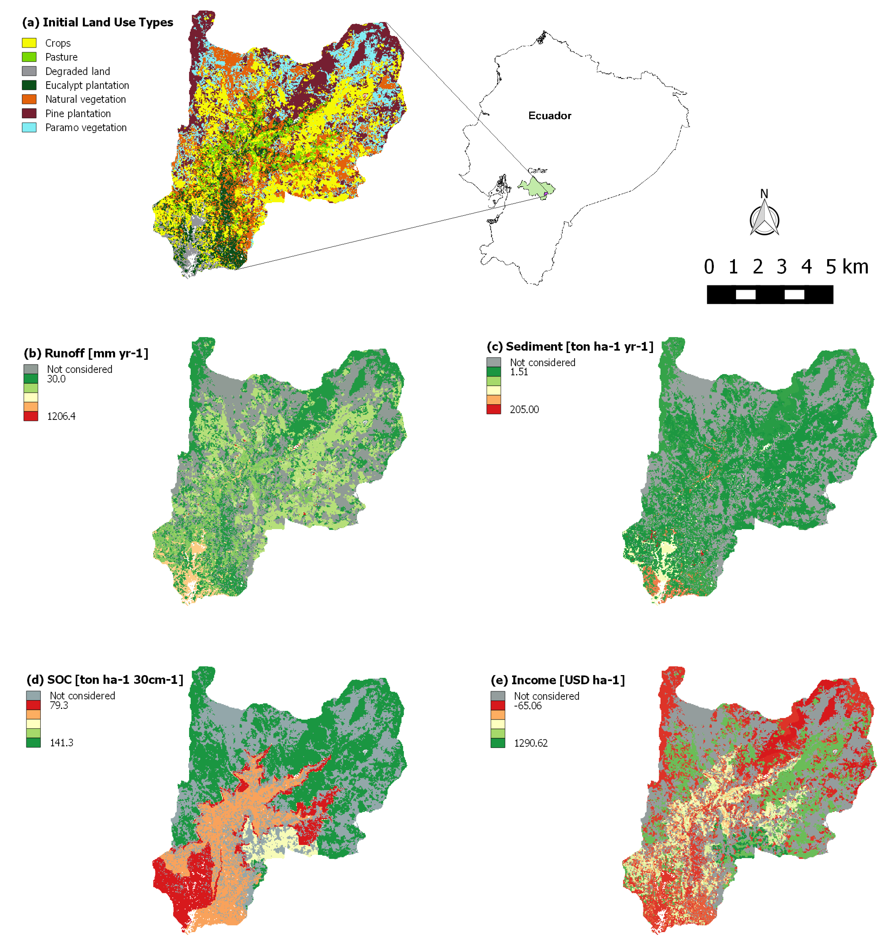Figure 1 displays the location of the Tabacay river catchment in Ecuador and in the province of Cañar along with the initial land use type distribution (iLUT) (Figure 1a). The remaining maps in Figure 1 show the land performance of the Tabacay catchment, as expressed by its runoff production (Figure 1b), sediment production (Figure 1c), stock of organic carbon in the soil (Figure 1d), and monetary income (Figure 1e). The stock of organic carbon in the biomass is not displayed in Figure 1 because it is assumed to be 0 for the full catchment at the initial situation.

For several reasons the improvement of land performance in the Tabacay catchment is a pertinent matter. First, Tabacay is a subcatchment of the Paute catchment, where one of the main complexes for hydroelectricity generation of Ecuador is located. Therefore it is important to take measures that decrease the sediment influx in the Tabacay river by mitigating its causing factors, local runoff and sediment production. The ultimate goal of such measures is to prevent river and reservoir sedimentation and the consequent shortening of the life span of this hydroelectricity complex. Additionally, the Tabacay river is used as the only source of drinking water for the city of Azogues, the capital of the province of Cañar, which is located around the outlet of the Tabacay catchment. Finally, agriculture is the predominant land use type in Tabacay, also on high altitude areas with steep slopes. This practice is known to affect negatively the provision of ecosystem services like water supply regulation and soil conservation ([22]).

Figure 1. (a) Initial (year 0) land use type distribution and location in Ecuador of the Tabacay catchment; and its initial environmental performance expressed in terms of (b) Runoff production; (c) Sediment production; (d) Soil Organic Carbon (SOC); and (e) Monetary income. The areas under páramo and natural vegetation were excluded from the study (see Section 3.2). These areas are displayed in gray in maps (b–e).

Figure 1. (a) Initial (year 0) land use type distribution and location in Ecuador of the Tabacay catchment; and its initial environmental performance expressed in terms of (b) Runoff production; (c) Sediment production; (d) Soil Organic Carbon (SOC); and (e) Monetary income. The areas under páramo and natural vegetation were excluded from the study (see Section 3.2). These areas are displayed in gray in maps (b–e).

3.2. Available Data

The major geodataset used in this study represents the Tabacay catchment as stratified in 417 land units. The definition of these land units is based on seven categorical characteristics as described in Table 1 ([23]).

Table 1. Land characteristics consider to stratify the Tabacay dataset into land units.

Initial Land Cover	Soil *	Precipitation	Slope	Lithology *	Land Curvature	Elevation
-	-	mm·Year−1	%	-	-	m asl
Crops	Suitable	<650	<25	Suitable	Convex	<3000
Pasture	With restrictions	650–1000	25–75	With restrictions	Straight	3000–3300
Degraded land	Unsuitable	>1000	>75	Unsuitable	Concave	>3300
Eucalypt forest
Native vegetation
Pine forest
Páramo

* Regarding suitability for forestry.

Table 1. Land characteristics consider to stratify the Tabacay dataset into land units.

Initial Land Cover	Soil *	Precipitation	Slope	Lithology *	Land Curvature	Elevation
-	-	mm·Year−1	%	-	-	m asl
Crops	Suitable	<650	<25	Suitable	Convex	<3000
Pasture	With restrictions	650–1000	25–75	With restrictions	Straight	3000–3300
Degraded land	Unsuitable	>1000	>75	Unsuitable	Concave	>3300
Eucalypt forest
Native vegetation
Pine forest
Páramo

* Regarding suitability for forestry.

Each of the characteristics in Table 1 is available as a polygon geodataset. In spatial terms, each land unit consists of a multi-polygon resulting from the overlay of all these geodatasets. In this sense, a land unit is a (possibly scattered) multi-polygon representing an area of homogeneous characteristics. Such multi-polygons are typically different from each other in terms of shape and size. For instance the smallest land unit has an area of 0.09 ha, while the largest is 210.6 ha. The average size of the considered land units amounts to 15.1 ha and the standard deviation of these land units is 30 ha.

The land cover páramo refers to neotropical andean wetlands normally covered by grassland and located between 3500 and 5000 m asl in the northern Andes ([24]). The land units covered by páramo as well as those covered by natural woody vegetation were excluded from the study, since it was considered that it is ecologically important that such land use types remain undisturbed. This filtered out 140 land units from the database, limiting the analysis to 277 land units (66%) that represent 41.83 km² (62.9%) of the Tabacay catchment area. Therefore, each of these land units is initially under one of five possible land covers (LUT before year 0): agriculture, grassland, degraded land, pine forest and eucalypt forest.

Land performance data for each of these 277 land units were retrieved from a previous study ([23]). Land performance, in this context, is expressed in terms of five on-site continuous attributes: runoff production (m³·ha⁻¹·year⁻¹), sediment production (ton·ha⁻¹·year⁻¹), stock of organic carbon in soil (SOC, ton·ha⁻¹·30 cm⁻¹), stock of organic carbon in biomass (BOC, ton·ha⁻¹) and monetary income (USD·ha⁻¹·year⁻¹ for crops and pasture, USD·ha⁻¹ for pine plantation and eucalypt plantation). Runoff and sediment production are expressed as yearly rate values, while SOC and BOC represent the stock of carbon existing in soil or biomass at a given point in time. Income values express the yearly difference between revenue and costs generated by crops and pasture, or the total net income (revenue-costs) that is earned from wood when a pine or eucalypt forest is harvested at a certain point in time. In the assessment of these income values no discount rate has been applied, hence they are not expressed as net present values. In addition to [23] and the present study, those attributes have already been used as indicators of land performance on ESS in other studies ([5,25]). Although, in general, information about any on-site performance attributes could be used as input data for BIOLP, in this specific case these five performance attributes were chosen since they are considered to be relevant for important ESS in the study area. For instance, following the ESS classification given by [26], sediment production influences food provision from crops (since soil erosion degrades soil fertility and crop productivity), fresh water provision (since suspended soil particles affect negatively the provision of drinking water), and erosion regulation. These ESS are of particular importance in the Tabacay catchment, given the importance of agriculture in the area and considering that the river Tabacay is used as a source of drinking water for towns in the neighbourhood. The relevance of SOC and BOC is given by their influence on climate regulation, while river discharge regulation is affected by the production of runoff.

For each land unit, information about these five performance attributes is available for its initial land cover ([22]), and for all other LUT. This database also contains estimated performance attribute values for pine or forest plantations of 10 and 30 years of age, for each land unit. The values corresponding to runoff production, sediment production and SOC, at years 0, 10, 20 and 30 for crops and pasture are assumed to remain at the same level over time. For these two LUT BOC is assumed to always be 0 and monetary income at each 10 years period corresponds to the sum of the yearly values.

3.3. Land Use Trajectories and Their Performance

The present study aims at determining, for each land unit, the land use trajectory that contributes to the optimal cumulative land performance of a region over 30 years. The term land use trajectory refers to a series of land use types (LUT) that are implemented sequentially within a time span of 30 years at 10 years intervals. Four LUT are considered: crops, pasture, pine plantation, and eucalypt plantation.

A land use trajectory for a land unit is defined as follows. First, one of the four considered LUT is assumed to be established at the initial year (year 0), and this LUT is kept in place until years 10. At this point the current LUT can be kept as such or be replaced by a different LUT. The LUT established at years 10 is again assumed to be kept until years 20, when it can be kept or changed to another LUT. Finally, the LUT implemented at years 20 is kept for the remaining 10 years period. Therefore, a land use trajectory is defined by an ordered sequence of three LUT that are to be implemented at 10 years intervals, starting at a certain reference year (year 0, relative time) and within the boundaries of a 30 years time span. Both the 30 years time span and the 10 years intervals at which a land use change may or may not occur were chosen considering the available data. An alternative, more flexible approach would have been to determine the specific point in time at which land use is changed as part of the decision process. In this case in addition to selecting the target LUT to apply, the specific year at which such land use change should occur would be determined. This approach is clearly much less restrictive than the definition of land use trajectory used in this article, however it would add more complexity to the model formulation and it would drastically increase the input data and computational requirements.

Any LUT present in a given land unit before year 0 is assumed to be replaced by the first LUT of the sequence corresponding to the land use trajectory. For instance, if the LUT before year 0 (or initial LUT, iLUT) is pine forest and the first LUT in a given land use trajectory is also pine forest, the existing forest is assumed to be cut and replanted instead of being continued. The same reasoning applies for the case of eucalypt forest. There are two possibilities at years 10 or 20 regarding previously existing forest: either the forest is kept in place and continued for the next time interval, or the trees are cut and replaced by crops, pasture, forest of a different tree species, or by a new forest of the same tree species. For instance, for a given land use trajectory that involves the implementation of eucalypt forest from year 0 to years 10, such forest can be continued (so that a 20 years old forest will be present at years 20), cut and replanted, or replaced by crops, pasture or pine forest. Each of these possibilities corresponds to a different land use trajectory. At years 30 any existing forest is assumed to be harvested. Likewise, crops and pasture can be either continued or replaced by a different LUT at years 10 or 20.

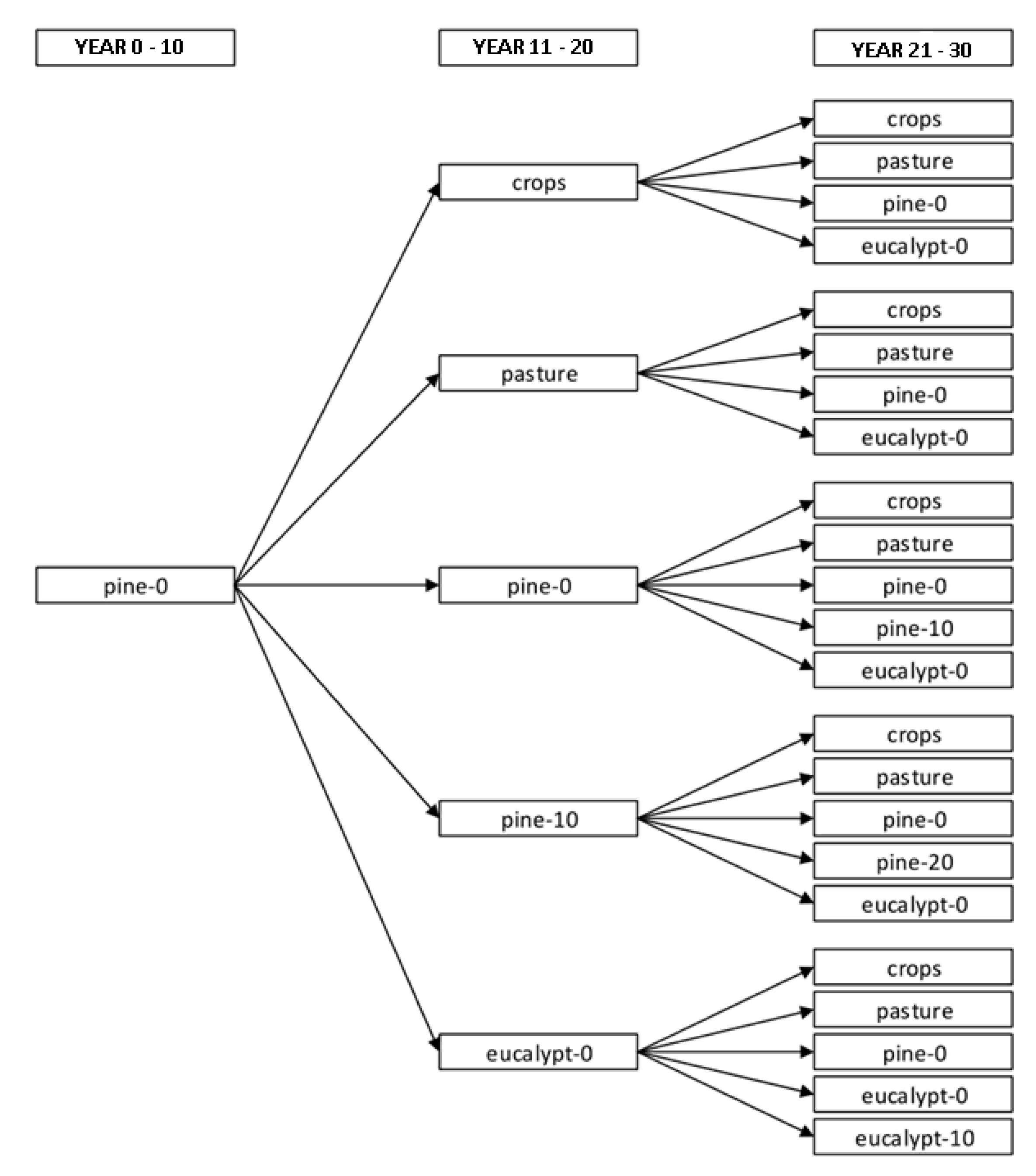
Following the principles sketched above, each possible sequence of the considered LUT defines a separate land use trajectory, which results in a total of 82 possible trajectories. A tree view of the 23 land use trajectories that start with pine forest is shown in Figure 2.

Figure 2. Tree view of all land use trajectories that start with pine forest. pine-X or eucalypt-X indicate a pine or eucalypt forest of X years of age, respectively.

Figure 2. Tree view of all land use trajectories that start with pine forest. pine-X or eucalypt-X indicate a pine or eucalypt forest of X years of age, respectively.

The performance level of a particular land unit at a given point in time depends on the current and, possibly, on previous LUT that have been established on it. Performance values were determined for each possible combination of the 277 land units and 82 land use trajectories. For each of these combinations, a performance value for each of the considered points in time (years 0, 10, 20 and 30) was determined. This procedure was applied to each of the five performance attributes under analysis. All values that were initially not available (values for years 10, 20 and 30 under crops and pasture and values for years 20 under pine and eucalypt) were computed from the information that was available in the database described in Section 3.2 following the assumptions summarized below.

• Land performance was assumed to remain constant under crops and pasture, i.e., performance values for years 0–10, 11–20 and 21–30 for crops and pasture were assumed to be the same;
• The land performance for a land unit under a 20 years old pine or eucalypt forest was linearly interpolated using the values corresponding to forests of 10 and 30 years of age (which were available in the database).

Based on these assumptions, performance values for years 0, 10, 20 and 30 were computed for each possible combination of land unit, land use trajectory and performance attribute. The results of the computation of these performance values are explained below for a sample land unit and trajectory. A characterization of the sample land unit is presented below, according to the different classes listed in Table 1:

• Area: 2.7 ha
• Initial land cover: Pasture
• Soil: Suitable with restrictions for forestry
• Lithology: Suitable for forestry
• Slope: 25%–75%
• Land curvature: Convex
• Elevation: 0–3000 m asl

Table 2 shows some statistical indicators aggregating all the trajectories corresponding to the sample land unit.

Table 2. Statistical indicators for the cumulative performance values over 30 years of all considered land use trajectories corresponding to the sample land unit.

Attribute	Unit	Minimum	Maximum	Average	Standard Deviation
Runoff	m3·ha−1	49,500	310,000	134,660	68,153
Sediment	ton·ha−1	187	6150	3024	1450
SOC	ton·ha−1·30cm−1	94	387	175	114
BOC	ton·ha−1	0	407	141	86
Income	USD·ha−1	2281	42,708	13,809	9341

Table 2. Statistical indicators for the cumulative performance values over 30 years of all considered land use trajectories corresponding to the sample land unit.

Attribute	Unit	Minimum	Maximum	Average	Standard Deviation
Runoff	m3·ha−1	49,500	310,000	134,660	68,153
Sediment	ton·ha−1	187	6150	3024	1450
SOC	ton·ha−1·30cm−1	94	387	175	114
BOC	ton·ha−1	0	407	141	86
Income	USD·ha−1	2281	42,708	13,809	9341

The sample land use trajectory involves replacing the initial pasture by pine forest (pine-0) at year 0, then replacing the 10 years old pine forest (pine-10) by eucalypt forest (eucalypt-0) at years 10, and then replacing the 10 years old eucalypt forest (eucalypt-10) by pasture at years 20, and keeping pasture between years 20 and 30.

Table 3 shows the runoff production values for the sample land unit, which correspond to the breakpoints of the time-performance curve for the sample land use trajectory, shown in the graph to the right.

Table 3. Runoff production values and graph for sample land unit and land use trajectory. Cumulative runoff production over 30 years: 78,750 m³·ha⁻¹.

Time Period	LUT	Runoff Production m3·ha−1·Year−1
iLUT	pasture	3000
from 0	pine-0	3000
until 10	pine-10	2100
from 10	eucalypt-0	2700
until 20	eucalypt-10	1950
from 20	pasture	3000
until 30	pasture	3000

Table 3. Runoff production values and graph for sample land unit and land use trajectory. Cumulative runoff production over 30 years: 78,750 m³·ha⁻¹.

Time Period	LUT	Runoff Production m3·ha−1·Year−1
iLUT	pasture	3000
from 0	pine-0	3000
until 10	pine-10	2100
from 10	eucalypt-0	2700
until 20	eucalypt-10	1950
from 20	pasture	3000
until 30	pasture	3000

Although according to the sample land use trajectory at year 0 LUT is changed to pine forest, the value of runoff production still corresponds to pasture, given that establishing a forest is assumed not to produce immediate effects in the runoff level. Runoff is assumed to evolve linearly until it reaches the known level corresponding to a 10 years old pine forest at years 10. At this point pine forest is replaced by a eucalypt forest, which causes runoff to immediately go back to 90% of its original level under pasture (since some vegetation is assumed to have developed under the trees during the period in which the pine forest was present, and such vegetation contributes to runoff reduction). Then runoff evolves until it reaches 90% of the known runoff corresponding to a 10 years old eucalypt forest. The factor of 90% is used at this point to take into account the vegetation that developed underneath the trees during the first period under pine forest. At years 20, the 10 years old eucalypt forest is converted to pasture, which causes runoff to immediately reach the level of the new LUT. Between years 20 and 30 the runoff level under pasture is assumed to remain constant. Since runoff production is a rate variable, which means that it expresses the amount of runoff that is produced on a yearly basis, the total cumulative runoff production over 30 years corresponds to the shaded area under the curve in the graph.

The breakpoint values of the performance curves and the corresponding graphs for the four remaining performance attributes of the sample land unit are shown in Table 4.

Table 4. Sediment, SOC, BOC and income performance values and graphs for sample land unit and land use trajectory.

Time Period	LUT	Sediment Production ton·ha−1·Year−1
iLUT	pasture	205
from 0	pine-0	205
until 10	pine-10	40.56
from 10	eucalypt-0	184.52
until 20	eucalypt-10	61.63
from 20	pasture	205
until 30	pasture	205
Time Period	LUT	SOC ton·ha−1·30 cm−1
iLUT	pasture	93.56
from 0	pine-0	93.56
until 10	pine-10	105.81
from 10	eucalypt-0	105.81
until 20	eucalypt-10	122.96
from 20	pasture	122.96
until 30	pasture	93.56
Time Period	LUT	BOC ton·ha−1
iLUT	pasture	0
from 0	pine-0	0
until 10	pine-10	116.22
from 10	eucalypt-0	0
until 20	eucalypt-10	55.78
from 20	pasture	0
until 30	pasture	0
Time Period	LUT	Income USD·ha−1
iLUT	pasture	0
from 0	pine-0	0
until 10	pine-10	760.19
from 10	eucalypt-0	0
until 20	eucalypt-10	1758.58
from 20	pasture	0
until 30	pasture	4356.47

Table 4. Sediment, SOC, BOC and income performance values and graphs for sample land unit and land use trajectory.

Time Period	LUT	Sediment Production ton·ha−1·Year−1
iLUT	pasture	205
from 0	pine-0	205
until 10	pine-10	40.56
from 10	eucalypt-0	184.52
until 20	eucalypt-10	61.63
from 20	pasture	205
until 30	pasture	205
Time Period	LUT	SOC ton·ha−1·30 cm−1
iLUT	pasture	93.56
from 0	pine-0	93.56
until 10	pine-10	105.81
from 10	eucalypt-0	105.81
until 20	eucalypt-10	122.96
from 20	pasture	122.96
until 30	pasture	93.56
Time Period	LUT	BOC ton·ha−1
iLUT	pasture	0
from 0	pine-0	0
until 10	pine-10	116.22
from 10	eucalypt-0	0
until 20	eucalypt-10	55.78
from 20	pasture	0
until 30	pasture	0
Time Period	LUT	Income USD·ha−1
iLUT	pasture	0
from 0	pine-0	0
until 10	pine-10	760.19
from 10	eucalypt-0	0
until 20	eucalypt-10	1758.58
from 20	pasture	0
until 30	pasture	4356.47

The meaning of the values for sediment is similar to those of runoff, that is, they express the yearly sediment production rates. Therefore, the cumulative sediment produced over 30 years corresponds to the shaded area under the curve in the graph. Since SOC is a stock variable, only the value present at years 30 is considered. This is indicated in the graph by the bold vertical bar. Although BOC is always present in a forest, which is indicated by the curve in the graph, BOC values are taken into account only when forest is harvested, which happens at years 10 and 20 in the sample trajectory. This principle is illustrated by the vertical bars in the graph. Income values have a mixed meaning. For crops and pasture, they express the yearly income. Therefore the area under the performance curve is considered for these LUT. For forest LUT, income values represent the amount of money obtained from wood, which is considered only when a forest is harvested. In all cases, the term income is used to refer to profit, that is, to the difference between the revenues and the costs associated to preparing the soil, and establishing and managing the plantation, be it crops, pasture or forest. In some cases, especially for forest LUT, costs may exceed revenues, which results in a negative income (loss).

3.4. An Integer Programming Model for Land Use Planning to Optimize Regional Land Performance

In [5] a mathematical programming model was introduced and applied to determine the land use configuration that would optimize regional land performance aggregated over a 30 years period without considering possible land use trajectories over time. The same model was used in the present study to find the land use trajectory that should be applied to every land unit in order to optimize the regionally-aggregated land performance of the full study area over a 30 years period. This model was formulated using a MCDM called Balanced Compromise Programming.

Compromise Programming (CP, [6]) is the reference method among the ideal-point based MCDMs. The first step in CP is to determine the ideal point, i.e., a hypothetical decision alternative that achieves the absolute optimal values for all criteria involved. Such an alternative is normally not a feasible solution, given the conflict among the criteria (improving one criterion degrades one or more of the others). CP gives preference to the alternatives that are closest to the ideal point. The distance between a given alternative and the ideal point is assessed in an n-dimensional space in which each of the n criteria correspond to a different dimension.

In its canonical form CP might favour unbalanced decision alternatives, that is, alternatives that perform well for certain criteria and poorly for others. In an attempt to alleviate this issue, a variant of CP called Balanced Compromise Programming (BCP) was introduced in [5]. BCP ensures that the balance among the level of achievement for the considered criteria plays also a role in the selection of an alternative. The application of BCP to a given decision problem results in a mathematical programming model.

Equations (1) to (4) correspond to the formulation of a BCP-derived mathematical programming model that is applied to the problem of finding a trajectory configuration that optimizes regional land performance.

$$\text{Min}\left[\lambda D+(1-\lambda ){\displaystyle \sum _{k=1}^q}{w}_k\frac{f_k^{*}-f_k\left(x\right)}{f_k^{*}-f_{\ast k}}\right]$$

(1)

subject to:

$${\displaystyle \sum _{j=1}^m}{x}_{ij}=1 \text{for} i=1,2,\dots ,n$$

(2)

$$w_k\frac{f_k^{*}-f_k\left(x\right)}{f_k^{*}-f_{\ast k}}\le D \text{for} k=1,2,\dots ,q$$

(3)

$$x_{ij}\in \{0,1\} \text{for} i=1,2,\dots ,n \text{and} j=1,2,\dots ,m$$

(4)

The constraints in Equation (4) restrict the decision variables of the model to take only on values 0 or 1. Therefore this formulation is an instance of an Integer Programming (IP) model. The acronym BIOLP, which stands for BCP-based IP land use planning model for the Optimization of regional Land Performance will be used throughout the rest of this article to refer to this model.

Equation (1) is the objective function of BIOLP. It comprises the balancing term and the distance (achievement) term. More specifically:

• x_ij are the decision variables of BIOLP. They indicate whether land use trajectory j should (x_ij = 1) or should not (x_ij = 0) be applied to land unit i.
• D is the maximum (weighted and normalized) deviation between any coordinate (criterion) of a given alternative and its counterpart in the ideal point;
• q is the number of considered criteria;
• w_k is the relative importance (weight) assigned to criterion k;
• $f_k^{*}$ and f_∗k are, respectively, the ideal and anti-ideal performance values corresponding to criterion k integrated over all considered land units in the study region;
• f_k(x) is the performance value for criterion k, integrated over all land units, corresponding to the decision alternative (candidate solution) under consideration. f_k(x) is given by a particular assignment of values to the decision variables x_ij;
• λ determines whether emphasis is given to a balanced solution (λ closer to 1) or to a solution that is close to the ideal point (λ closer to 0).

In Equation (1) the distance between a given alternative and the ideal point ($f_k^{*}-f_k\left(x\right)$) is divided by the full range for criterion k, that is, the difference between its ideal and anti-ideal values ($f_k^{*}-f_{\ast k}$). In this way the distance for criterion k is normalized, so that it can be combined in the sum with the distances corresponding to the other criteria. The normalized distance is also multiplied by w_k, which represents the relative importance (weight) assigned to criterion k. When the objective function is minimized, both the distance to the ideal point and the maximum deviation from any of its coordinates will be minimized, producing a solution that is at the same time close to the ideal and balanced considering the different criteria (depending on the value of λ).

Equations (2)–(4) are the constraints of BIOLP. The constraints in Equation (2) require that only a single land use trajectory j is assigned to land unit i. In these constraints m represents the total number of land use trajectories (82), while n corresponds to the number of land units (277). Therefore, the constraints in Equation (2) express that only 1 out of 82 decision variables corresponding to land unit i can be equal to 1, while all the other 81 variables are set to 0.

Equation (3) defines D as the maximum (weighted and normalized) deviation among the coordinates (performance attributes) of an alternative and their counterparts in the ideal point. D is a (non-decision) variable of the model, for which its value is to be minimized as part of the objective function (Equation (1)). On the other hand, the constraint in Equation (3) requires the deviation from the ideal point for each and every criterion to be less than or equal to D. Given the conflict among criteria (enhancing one of them degrades some others), the minimum possible value for D will be reached when the decision variables (x_ij) are assigned a value in such a way that the deviations from the ideal point for all criteria are similar. This situation will occur only when full emphasis is given to a balanced solution (λ = 1).

Any feasible solution (decision alternative) to BIOLP indicates a specific land use trajectory configuration over the considered land units. BIOLP then selects the land use trajectory configuration that optimizes regional land performance. In our study the criteria correspond to the performance attributes under consideration: runoff, sediment, SOC, BOC and income.

3.5. Sensitivity Analysis

A sensitivity analysis was performed on BIOLP through a series of tests outlined below. Each of them addressed a different aspect of BIOLP:

• Reference scenario;
• Sensitivity to uncertainty in the input data;
• Sensitivity to parameter settings;
• Performance thresholds.

3.5.1. Reference Scenario

In the reference scenario the input database detailed in Section 3.2 was used, λ was set to 0.5 to indicate that the same importance is given to a balanced solution and to the minimization of the distance to the ideal point, and equal weights (0.2) were assigned to all performance attributes. The output of BIOLP for this scenario was used as a reference for assessing the results in the remaining phases.

3.5.2. Model Sensitivity to Uncertainty in the Input Data

Given the imperfections of the available database and considering all the assumptions used to handle the missing data, it was considered relevant to gain insights in the behaviour of BIOLP under conditions of uncertainty in the input data. To this end, random “perturbations” were introduced in the performance curves (Table 3 and Table 4). Such perturbations consisted in randomly selecting a value from a range of ± 10% around the original breakpoint values in the curves and using this value as the new breakpoint. To perform a full perturbation, this step was repeated independently for every breakpoint in every land use trajectory for all land units in the database. Ten full perturbations were performed to produce the same number of different versions of the input database. BIOLP was then executed for each of these versions and the outcomes were assessed in terms of their distance to the ideal point and in comparison to the results for the reference scenario.

3.5.3. Model Sensitivity to Parameter Settings

BIOLP parameters comprise λ and one weight (relative importance) for each of the performance attributes. At this stage, the model performance for six different values of λ in the range from 0 (exclusive emphasis on minimization of distance to the ideal point) to 1 (exclusive emphasis on obtaining a balanced solution) was tested, using a step of 0.2, i.e., λ was set successively to 0, 0.2, 0.4, 0.6, 0.8 and 1, while keeping all weights fixed at a value of 0.2. To assess the sensitivity of the model to the weight parameters, five separate tests were performed. In each of these tests, the weight assigned to one performance attribute was set to 0.6 while the weights for all other attributes were set to 0.1. In these tests the value for λ was fixed to 0.5.

3.5.4. Performance Thresholds

BIOLP can accommodate requirements for one or more performance attributes (not) to exceed certain predefined threshold values. Such requirements can be expressed in the form of additional constraints in the model. Since in BIOLP (Equations (1)–(4)) f_k(x) represents the performance value for attribute k integrated over all land units, a performance threshold constraint takes the form f_k(x) ≤ u for an attribute to be minimized, or f_k(x) ≥ u for an attribute to be maximized, where u represents a user defined threshold. In this specific case, monetary income and carbon stock were chosen to illustrate the use of such performance thresholds.

4. Results

4.1. Ideal and Anti-Ideal Points

The first step in CP and BCP is to compute the ideal and anti-ideal points. The ideal point is a hypothetical decision alternative for which the coordinate value of each of its attributes corresponds to the absolute optimum that such attribute can reach, that is, each of the coordinates of the ideal point is obtained by optimizing the corresponding attribute independently from the others, thus the conflict among attributes is neglected. In this case the ideal point coordinates were computed by determining, for each land unit, the trajectories resulting in (i) minimum runoff; (ii) minimum sediment; (iii) maximum SOC; (iv) maximum BOC; and (v) maximum income. Then, these optimal performance values for each attribute was summed up over all land units in order to compute the regionally integrated ideal point coordinate. The anti-ideal point was computed in a similar way, only that the anti-optimal values were chosen for each combination of land unit and attribute. The resulting ideal and anti-ideal coordinates are listed in Table 5.

Table 5. Ideal and anti-ideal points for the Tabacay database. Values are aggregated over a 30 years period.

Attribute	Ideal Value	Anti-Ideal Value	Unit
Runoff	72,611,012	772,071,110	m3
Sediment	95,675	1,733,716	ton
SOC	1,260,563	77,853	ton
BOC	813,446	0	ton
Income	214,059,996	−6,378,626	USD

Table 5. Ideal and anti-ideal points for the Tabacay database. Values are aggregated over a 30 years period.

Attribute	Ideal Value	Anti-Ideal Value	Unit
Runoff	72,611,012	772,071,110	m3
Sediment	95,675	1,733,716	ton
SOC	1,260,563	77,853	ton
BOC	813,446	0	ton
Income	214,059,996	−6,378,626	USD

4.2. Reference Scenario

The settings for the reference scenario involve using the original input database, with λ = 0.5 (equal emphasis on minimization of distance to the ideal point on the one hand and balanced solution on the other hand), and assigning the same relative importance to each of the attributes (all weights set to 0.2).

The distribution of land use trajectories that optimizes land performance resulting from the application of BIOLP for the reference scenario consisted in the distribution of 27 out of 82 trajectories over the considered land units. Table 6 lists the seven trajectories in this distribution that cover the largest area in the Tabacay catchment.

Table 6. Distribution of land use trajectories over the Tabacay catchment that optimizes land performance, obtained by applying BIOLP for the reference scenario (7 out of 27 assigned trajectories are reported).

Land Use Trajectory	Area Covered (%)	Land Unit Count
pasture → eucalypt-0 → crops	27.7	25
pine-0 → pine-10 → pine-20	23.8	80
eucalypt-0 → eucalypt-0 → pine-0	12.3	4
pasture → eucalypt-0 → pine-0	12.0	5
eucalypt-0 → eucalypt-0 → eucalypt-0	10.8	24
crops → crops → crops	3.1	54
pasture → pine-0 → eucalypt-0	2.9	7
Total	92.6	199

Table 6. Distribution of land use trajectories over the Tabacay catchment that optimizes land performance, obtained by applying BIOLP for the reference scenario (7 out of 27 assigned trajectories are reported).

Land Use Trajectory	Area Covered (%)	Land Unit Count
pasture → eucalypt-0 → crops	27.7	25
pine-0 → pine-10 → pine-20	23.8	80
eucalypt-0 → eucalypt-0 → pine-0	12.3	4
pasture → eucalypt-0 → pine-0	12.0	5
eucalypt-0 → eucalypt-0 → eucalypt-0	10.8	24
crops → crops → crops	3.1	54
pasture → pine-0 → eucalypt-0	2.9	7
Total	92.6	199

The first land use trajectory in Table 6 indicates that pasture is implemented at year 0 and kept until years 10, when it is replaced by a eucalypt forest, which is kept until years 20, when the 10 years old eucalypt forest is replaced by crops, which is in turn kept until the end of the 30 years time span. A similar interpretation can be made for the remaining land use trajectories in the first column of Table 6. The second and third columns of this table are the percentage of the full catchment area (excluding land units under páramo and natural vegetation) and the number of land units in which the corresponding trajectory should be implemented according to the output of BIOLP. Figure 3 shows the spatial distribution over the Tabacay catchment of the land use trajectories listed in Table 6.

In Table 6 and Figure 3a relative predominance of forest trajectories over crops and pasture is apparent. This fact is as expected since, in general, pine and eucalypt forests result in higher performance levels for most of the attributes taken into account. The extreme case is BOC, which is assumed to be always 0 for crops and pasture. Higher performance levels for forest LUT are also observed for runoff, sediment and SOC. On the other hand, income values are typically higher for crops and pasture, which probably explain the few occurrences of these LUT among the trajectories that cover most of the Tabacay area.

Figure 3. Distribution of land use trajectories over the Tabacay catchment that optimizes land performance, obtained by applying BIOLP for the reference scenario. The category “Other trajectories” in the legend comprises 20 different trajectories that were assigned by BIOLP to relatively small areas.

Figure 3. Distribution of land use trajectories over the Tabacay catchment that optimizes land performance, obtained by applying BIOLP for the reference scenario. The category “Other trajectories” in the legend comprises 20 different trajectories that were assigned by BIOLP to relatively small areas.

The normalized distance to each coordinate of the ideal point can be used as an indicator of the “quality” of a solution produced by BIOLP. This indicator is a continuous value ranging between 0, when the coordinate of the solution is equal to that of the ideal point, and 1, when the coordinate of the solution is equal to that of the anti-ideal point (second term of BIOLP’s objective function, Equation (1)). The normalized distances to the ideal point corresponding to the solution for the reference scenario are listed in Table 7.

Table 7. Normalized distances to the ideal point corresponding to the optimal distribution of trajectories produced by BIOLP for the reference scenario.

Performance Attribute	Normalized Distance
Runoff	0.488
Sediment	0.228
SOC	0.093
BOC	0.315
Income	0.488

Table 7. Normalized distances to the ideal point corresponding to the optimal distribution of trajectories produced by BIOLP for the reference scenario.

Performance Attribute	Normalized Distance
Runoff	0.488
Sediment	0.228
SOC	0.093
BOC	0.315
Income	0.488

It can be seen in Table 7 that the solution corresponding to runoff and income for the reference scenario is halfway between the anti-ideal and the ideal points, while the normalized distances for the other attributes are smaller, which is particularly noticeable in the case of SOC, for which the reference solution is less than 10% away from the ideal.

The existence of multiple optimal solutions depends on the specific characteristics of the problem and its corresponding formulation as a mathematical programming model. However the large quantity of degrees of freedom (277 land units, 82 possible land use trajectories, 5 performance attributes) in the studied case makes the existence of multiple optimal configurations of land use trajectories (for the same scenario) very unlikely. On the other hand, there may be several solutions that are close to the optimal one. To investigate the possible existence of close-to-optimal configurations we first computed the least optimal solution, i.e., the land trajectory distribution which results in a regional performance that is closest to the anti-ideal point. Next we assessed trajectory configurations of which we hypothesized that they achieve close-to-optimal ecosystem service delivery at the basin scale. The first one corresponds to selecting the land unit with the smallest area (0.09 ha) and replacing the land use trajectory assigned for optimality (i.e., pine-0 → pine-0 → pasture) by an arbitrary trajectory (agricultural land use over the full time span, crops → crops → crops). A similar approach was taken for the second trajectory configuration but here the land unit occupying the largest area (210.6 ha) in the Tabacay basin was selected and its optimal trajectory replaced by crops → crops → crops. The full performance range is assessed as the Euclidean distance between the normalized coordinates of the optimal solution for the reference scenario (0.488, 0.228, 0.907, 0.685, 0.512) and their counterparts for the least optimal (closest to anti-ideal point) solution (0.671, 0.672, 0.026, 0.264, 0.328). The coordinates for both the optimal and least-optimal solutions are normalized in the range [0, 1] with respect to the corresponding coordinates of the anti-ideal and ideal points. They must not be confused with the normalized distances to the ideal point (Table 7). The normalized Euclidean distance between the optimal and least optimal solution equals 1.104 (unitless, -). The distance between the optimal solution and the first disturbed configuration equals 0.0005 (-) while the second disturbed configuration is at a distance of 0.0397 (-) from the optimal solution. The latter two distances represent 0.05% resp. 3.59% of the range and indicate indeed that land use trajectory configurations exist that deliver ecosystem services to almost the same extent as the optimal one. A similar analysis of the performance of all possible trajectory configurations was beyond the scope of this paper but potentially provides interesting information to land use planners on the impact, in terms of regionally integrated ecosystem service delivery, of land use plans that deviate from the optimal configuration.

4.3. Sensitivity of BIOLP to Uncertainty in the Input Database

This section reports on the effects that controlled changes in the input database produce on the output of BIOLP. In particular, BIOLP was executed 10 times, using a different version of the input database in each test. To produce the modified input database for each run, a random perturbation was introduced in the data.

The indicator used to compare the level of agreement between the BIOLP output for two different scenarios is the coincidence index and it is expressed as the ratio between the number of land units for which both BIOLP runs suggested the same land use trajectory and the total number of land units under consideration. The coincidence index is a value between 0 (no agreement for any land unit) and 1 (agreement for all land units). The coincidence index was computed to determine the agreement between the output of BIOLP for the reference scenario and the results of each of the 10 runs corresponding to the stochastically modified versions of the input database. The coincidence index for these 10 tests ranges from 0.68 to 0.76 with an average value of 0.72.

In an extreme case, a land unit might be assigned a different trajectory in each of the 11 tests (one test for the reference scenario and ten for the randomly modified databases). On the other hand, it is possible that the same trajectory is assigned to a given land unit in all tests. Table 8 lists the number of land units that were assigned each possible number of distinct trajectories.

Table 8. Number of distinct trajectories assigned and corresponding land unit count.

Distinct Trajectories	Land Unit Count	Percentage
1	106	38.3
2	55	19.9
3	47	17.0
4	35	12.6
5	15	5.4
6	7	2.5
7	4	1.4
8	3	1.1
9	3	1.1
10	1	0.3
11	1	0.3
Total	277	100

Table 8. Number of distinct trajectories assigned and corresponding land unit count.

Distinct Trajectories	Land Unit Count	Percentage
1	106	38.3
2	55	19.9
3	47	17.0
4	35	12.6
5	15	5.4
6	7	2.5
7	4	1.4
8	3	1.1
9	3	1.1
10	1	0.3
11	1	0.3
Total	277	100

Table 8 shows that 106 out of 277 land units were assigned the same trajectory in all tests. Of the remaining land units, 55 were assigned two distinct trajectories. In general most land units were assigned a relatively low number of distinct trajectories throughout all tests, which is an indicator of the limited impact that the imposed variations of the input data have on the results of BIOLP.

4.4. Sensitivity of BIOLP to Different Parameter Settings

The impact that different parameter settings have on the results produced by BIOLP is reported in this section. Before running BIOLP, the values for a number of parameters must be set, namely, λ and one weight for each considered attribute.

To evaluate the model sensitivity to λ, the original version of the database was used as input and the weights for all attributes were fixed to 0.2. Then BIOLP was executed six times, varying λ from 0 (full priority to the minimization of the distance to the ideal point) to 1 (full priority to a balanced solution) in 0.2 steps. Table 9 lists the coincidence index when comparing the output of these six tests with the output for the reference scenario.

Table 9. Coincidence index values comparing the output of BIOLP for the reference scenario and for scenarios using different values for the λ parameter (all weights were fixed to 0.2).

λ Value	Coincidence Index
0.0	0.76
0.2	0.84
0.4	0.94
0.6	0.92
0.8	0.73
1.0	0.39

Table 9. Coincidence index values comparing the output of BIOLP for the reference scenario and for scenarios using different values for the λ parameter (all weights were fixed to 0.2).

λ Value	Coincidence Index
0.0	0.76
0.2	0.84
0.4	0.94
0.6	0.92
0.8	0.73
1.0	0.39

Taking apart the case in which a fully balanced solution was required, the values for the coincidence index for all other cases are relatively high, which indicates a limited sensitivity of BIOLP with respect to the λ parameter. The low coincidence value in case of a fully balanced solution follows from the fact that the balance level of the reference scenario solution is rather limited, which is exemplified in Table 7 by the difference between the distances corresponding to runoff and income (slightly below 0.5) on the one hand, and the one for SOC (<0.1) on the other hand.

To illustrate the influence of the λ parameter on the balance of the resulting solution, Table 10 reports the normalized distances for the scenarios corresponding to λ = 0 and λ = 1.

Table 10. Normalized distances of the solution produced by BIOLP for λ = 0 and λ = 1 (all weights were fixed to 0.2).

Performance Attribute	Normalized Distance
	λ = 0	λ = 1
Runoff	0.318	0.445
Sediment	0.205	0.250
SOC	0.093	0.442
BOC	0.259	0.445
Income	0.685	0.445

Table 10. Normalized distances of the solution produced by BIOLP for λ = 0 and λ = 1 (all weights were fixed to 0.2).

Performance Attribute	Normalized Distance
	λ = 0	λ = 1
Runoff	0.318	0.445
Sediment	0.205	0.250
SOC	0.093	0.442
BOC	0.259	0.445
Income	0.685	0.445

To evaluate the impact of different weight settings on the output of BIOLP, a set of five tests was performed. In each test the weight corresponding to one of the performance attributes was set to 0.6, while all other weights were fixed to 0.1. λ was set to 0.5 in all cases. Table 11 lists the coincidence index values for these tests when comparing their output to the outcome for the reference scenario.

Table 11. Coincidence index values comparing the output of BIOLP for the reference scenario and for scenarios using different weight settings (λ was set to 0.5).

Weight Setting	Coincidence Index
weightrunoff = 0.6, all other weights = 0.1	0.39
weightsediment = 0.6, all other weights = 0.1	0.54
weightSOC = 0.6, all other weights = 0.1	0.69
weightBOC = 0.6, all other weights = 0.1	0.51
weightincome = 0.6, all other weights = 0.1	0.35

Table 11. Coincidence index values comparing the output of BIOLP for the reference scenario and for scenarios using different weight settings (λ was set to 0.5).

Weight Setting	Coincidence Index
weightrunoff = 0.6, all other weights = 0.1	0.39
weightsediment = 0.6, all other weights = 0.1	0.54
weightSOC = 0.6, all other weights = 0.1	0.69
weightBOC = 0.6, all other weights = 0.1	0.51
weightincome = 0.6, all other weights = 0.1	0.35

In general the coincidence values in Table 11 are lower than the ones corresponding to the sensitivity tests for λ. This behaviour can be explained by the fact that, in each of the tests reported in Table 11, all five weight parameters were changed with respect to the reference scenario, while for the tests involving the sensitivity to λ, a single parameter was adjusted in each case. In this contexts it must be acknowledged that when a higher weight is given to an attribute with a low normalized distance for the reference solution, the correspondence with the reference configuration of trajectories decreases. Consider for example the case in which more importance is given to runoff (reference normalized distance = 0.488). In that case, less than 40% of the land units are assigned the same trajectory with respect to the reference scenario. On the other hand, if emphasis is given to SOC (reference normalized distance = 0.093), almost 70% of the land units are assigned the same trajectory as for the reference. As further illustration, Table 12 lists the normalized distances for the solution produced by BIOLP when the weight for runoff is set to 0.6 and all other weights are fixed to 0.1.

Table 12. Normalized distances of the solution produced by BIOLP for weight_runoff = 0.6 and all other weights fixed to 0.1 (λ was set to 0.5).

Performance Attribute	Normalized Distance
Runoff	0.042
Sediment	0.144
SOC	0.485
BOC	0.394
Income	0.901

Table 12. Normalized distances of the solution produced by BIOLP for weight_runoff = 0.6 and all other weights fixed to 0.1 (λ was set to 0.5).

Performance Attribute	Normalized Distance
Runoff	0.042
Sediment	0.144
SOC	0.485
BOC	0.394
Income	0.901

4.5. Performance Thresholds

The possibility of accommodating performance thresholds in BIOLP was tested using the attributes monetary income and carbon stock in the soil and in the biomass. The first performance threshold constraint was defined to require income to be at least as high as 10% of the minimum amount of money that is required to fulfil the basic needs of all inhabitants in the Tabacay catchment. To compute the income threshold value several information elements were considered. The total population of Tabacay for every year in the period 2015–2045 was estimated using census information available for 2010 and the population projections for the period 2011–2020 ([27]). Furthermore, information about the minimum income required by a family in the province of Cañar to fulfil its basic needs was retrieved as monthly values for the current and past years. Using this information as a reference, the yearly income required by a family in Tabacay was estimated for each year the period 2015–2045. The total income required to cover the basic expenses of the full population of Tabacay for the period 2015–2045 was then computed using Equation (5).

$$u_{income}={\displaystyle \sum _{y=2015}^{2045}}{f}_y{i}_y$$

(5)

where u_income is the value for the income threshold, f_y is the number of families living in Tabacay at year y (an average family size of four was assumed), and f_y is the minimum income required by a family in Tabacay at year y.

From Equation (5) the minimum amount of money required to fulfil the basic needs of the population of Tabacay is above 1.58 billion USD, whereas the income coordinate of the ideal point (maximum income possible) is around 214 million USD. This means that, when considering only the income from crops, pasture, pine plantation and eucalypt plantation in Tabacay, at most 13.6% of the total amount of money required to cover the basic needs of the population can be generated. The performance constraint for income included in BIOLP considered a threshold of 158 million USD, i.e., 10% of the value resulting from Equation (5).

From Table 7, it can be seen that the solution generated by BIOLP for the reference scenario results in a SOC stock deviating 9.3% and a BOC stock deviating 31.5% from their corresponding ideal values. Since the solution performance regarding SOC was considered relatively high, a performance threshold constraint was included in BIOLP to require that such level is maintained (SOC ≥ 1,150,571 ton). On the other hand, a performance threshold was defined to require that the deviation from the ideal concerning BOC improves from 31.5% until at least 25% (BOC ≥ 610,000 ton).

The resulting (partial) distribution of trajectories over Tabacay after applying BIOLP to the reference scenario and considering the performance threshold constraints described above is summarized in Table 13. The corresponding spatial distribution is displayed in Figure 4.

Table 13. Distribution of land use trajectories over the Tabacay catchment that optimizes land performance, obtained by applying BIOLP for the reference scenario and considering income and carbon stock thresholds (5 out of 25 assigned trajectories are reported).

Land use Trajectory	Area Covered (%)	Land Unit Count
pine-0 → pine-10 → pine-20	25.1	73
eucalypt-0 → eucalypt-0 → crops	20.0	12
eucalypt-0 → eucalypt-0 → pine-0	18.0	7
crops → crops → crops	16.6	98
eucalypt-0 → eucalypt-0 → eucalypt-0	13.3	36
Total	93.0	226

Table 13. Distribution of land use trajectories over the Tabacay catchment that optimizes land performance, obtained by applying BIOLP for the reference scenario and considering income and carbon stock thresholds (5 out of 25 assigned trajectories are reported).

Land use Trajectory	Area Covered (%)	Land Unit Count
pine-0 → pine-10 → pine-20	25.1	73
eucalypt-0 → eucalypt-0 → crops	20.0	12
eucalypt-0 → eucalypt-0 → pine-0	18.0	7
crops → crops → crops	16.6	98
eucalypt-0 → eucalypt-0 → eucalypt-0	13.3	36
Total	93.0	226

Figure 4. Distribution of land use trajectories over the Tabacay catchment that optimizes land performance, obtained by applying BIOLP for the reference scenario considering income and carbon stock thresholds. The category “Other trajectories” in the legend comprises 20 different trajectories that were assigned by BIOLP to relatively small areas.

Figure 4. Distribution of land use trajectories over the Tabacay catchment that optimizes land performance, obtained by applying BIOLP for the reference scenario considering income and carbon stock thresholds. The category “Other trajectories” in the legend comprises 20 different trajectories that were assigned by BIOLP to relatively small areas.

In Table 13 and Figure 4 there is a clear predominance of forest land use trajectories, especially trajectories involving eucalypt plantation. This fact is as expected, considering the thresholds set for carbon stocks and that non-forest LUT are assumed to always have a BOC of 0. The frequent appearance of eucalypt follows leads us to conclude that this species presents a good performance regarding carbon sequestration and income. On the other hand, the appearance of the trajectory involving an agricultural land use during the full 30 years time span may be explained by the requirement to fulfil the income threshold. Table 14 reports the normalized distances to the ideal point corresponding to the scenario with income and carbon stock performance thresholds.

Table 14. Normalized distances of the solution produced by BIOLP when considering income and carbon stock thresholds.

Performance Attribute	Normalized Distance
Runoff	0.805
Sediment	0.343
SOC	0.093
BOC	0.250
Income	0.255

Table 14. Normalized distances of the solution produced by BIOLP when considering income and carbon stock thresholds.

Performance Attribute	Normalized Distance
Runoff	0.805
Sediment	0.343
SOC	0.093
BOC	0.250
Income	0.255

5. Discussion

BIOLP is an Integer Programming model that was derived from the application of the Balanced Compromise Programming MCDM. The general aim of BIOLP is to determine how a set of land use types should be distributed over space and time in order to optimize the multi-dimensional regional performance of land. In this particular case, BIOLP was applied to a database that consists of a set of land units representing the catchment of the Tabacay river, located in Ecuador. This database contains values corresponding to five performance attributes for each possible combination of land units and land use types: runoff production, sediment production, stock of soil organic carbon (SOC), stock of biomass organic carbon (BOC), and monetary income. These performance values represent the state of affairs in the catchment at a reference point in time (year 0), and 10, 20 and 30 years after. Four different land use types (crops, pasture, pine plantation and eucalypt plantation) and 277 land units are considered. Any of these land use types can be applied to a land unit either at years 0, 10, or 20. A land use sequence, or trajectory, is defined by the combination and order in which these land use types are established. BIOLP was applied in this study to determine the land use trajectory, over a 30 years time span, that should be implemented in each land unit in order to optimize the regional land performance expressed in terms of the five attributes listed above.

In [5] BIOLP was applied to solve a problem that involved determining the distribution of a number of land use types over the Tabacay catchment in order to optimize the multi-dimensional land performance at a regional scale. In that work it is assumed that the land use type assigned to any land unit is kept during the full period of 30 years. In this sense, the land use configurations resulting from the application of BIOLP in [5] are static. In the present work, the application of BIOLP was taken one step further, by incorporating the temporal dimension. The restriction of allowing a land use change to occur only at the beginning of the considered period is no longer present. Instead, land use changes may (but must not) occur at 10 years intervals within the 30 years period. From this perspective and given the definition of trajectory, which implicitly suggests the possibility of land use changes after preset intervals, the application of BIOLP in the present study can be considered a generalization of the work reported in [5]. Although time was discretized into relatively coarse periods, this work can be considered as a first step towards more flexible models that allow to tackle a broader category of problems.

An apparent predominance of forest land use types was observed among the land use trajectories suggested by BIOLP for the Tabacay catchment. This fact is a result of the superior performance of forest over crops and pasture, which is particularly evident for the case of BOC, but also notorious for runoff and sediment production and for SOC. On the other hand, land performance corresponding to agriculture and pasture exceeds forest in terms of income, which is the reason why non-forest land use types are sporadically present in the solution provided by BIOLP.

It is obvious, however, that the fact that the values for monetary income were not corrected for devaluation over time by applying a discount rate has an impact on the absolute results, i.e., the location in feature space of the ideal point and the distance to the ideal point of the optimal (and other) land use trajectory configurations. For example, a constant yearly discount rate of 5% would make the income coordinate of the ideal point shift from an assumed 1000 USD to 950 USD after one year, 598.70 USD after 10 years, 358.50 USD after 20 years and 214.60 USD after 30 years. Moreover, the discounting makes a single land use type selected as the second component of a land use trajectory to have a lesser absolute contribution to the overall land performance than when it is selected as the first component and a higher contribution with respect to when it is selected as the third component. This behavior is not applicable though to the four other ESS considered in this study. However, since a same discount rate would be applied to the income values generated from all land use types that can be part of a trajectory, the nature and sequence of land use types in the selected trajectories will mostly not be affected.

In particular, given a specific trajectory configuration resulting from the application of BIOLP to a given scenario in which the discount rate was not taken into account, the only trajectories that would be significantly affected, when discount rates are applied, are the ones that contain a high performing land use type (LUT) in terms of income (e.g., crops or pasture) during the second or third time period (i.e., from years 11 to 20 or 21 to 30). Such trajectories will be presumably replaced by others in which high income LUT appear in the first or second intervals of the time span (i.e., 0–10 or 11–20). This is based on the fact that such changes do not affect in a considerable way the performance attributes other than income. For instance, considering the sample land unit, for which its performance is illustrated in Table 3 and Table 4, if pasture (which performs better in terms of income than any forest LUT) was established in the first time interval (0–10) instead of the final interval (21–30), such trajectory change would not affect the total runoff produced during the full time span. The same can be said for the case of sediment and BOC. On the other hand, for trajectories involving cutting and replanting forest of different tree species in consecutive periods, runoff and sediment values will effectively change when the trajectory is modified in such a way that the periods under forests are not consecutive anymore or the tree species used for the consecutive periods are swapped.

Applying the reasoning described above to the solution for the reference scenario described in Table 6, one can argue that the only trajectory affected when applying discount rates would be the first one (pasture → eucalypt-0 → crops). In that hypothetical case, this trajectory might be replaced by one in which crops appears earlier, possibly in the first time interval. The last trajectory in Table 6 (pasture → pine-0 → eucalypt-0) might also be replaced by one in which pine and eucalypt are swapped, given the higher performance in terms of income that is normally found in eucalypt forest over pine plantations. The other trajectories in Table 6 would presumably remain the same, although the specific land units to which it is applied and, thus, the area covered by each of the trajectories might change. In summary, some of the selected trajectories will change when considering discount rates in income, although such changes will not have a major effect on the overall trajectory configuration suggested by BIOLP for the whole study region.

Ten different tests of BIOLP were performed, using at each time a randomly modified version of the original database, with the aim of analyzing the behaviour of this model under simulated conditions of uncertainty in the input data. In all these tests, around 70% of the land units were assigned the same trajectory as the case in which the original database was used. This fact indicates a relatively low sensitivity of the output of BIOLP with respect to imposed variations in the input database, considering that all performance values were randomly modified within a restricted range (±10% of the original performance value). It is indeed expected that the similarity in the results decreases when the range of variation is enlarged. Another indicator of this sort of stability of the output of BIOLP is that around 38% of the land units were assigned the same trajectory in all tests, with an additional 20% being assigned only two distinct trajectories. In general, most land units were assigned a limited number of distinct trajectories when using different versions of the original database.

In addition to the sensitivity of BIOLP to simulated uncertainty in the input data, the impact of different parameter settings on its results was also assessed. The functioning of BIOLP depends on several parameters. The first parameter is λ, which indicates whether the priority is to find the solutions that are the closest to the absolute optimal (λ closer to 0) or a solution that achieves a balanced level for all performance attributes under consideration (λ closer to 1). In addition to λ, one weight parameter is provided for each performance attribute to denote the relative importance that such attribute has for the decision maker. To evaluate the sensitivity of BIOLP to different parameter settings, several tests were executed varying λ and the set of weights independently within their full allowed range ([0, 1]).

The changes on the results when varying λ between 0 and 0.8 were confined to a range of 25% with respect to the case when λ was set to 0.5, which indicates that the sensitivity of BIOLP to λ is relatively restricted, even for drastic variations. When full balance of the solution was required (λ = 1) the difference with regard to the reference increased to 60%, which means that the fully balanced solution is rather far from the reference in the solution space. This fact is clearly revealed when contrasting Table 7 and Table 10. With λ = 1 (balanced solution is an absolute requirement), the overall deviation from the ideal point is largest, followed by λ = 0.5 (reference scenario) and λ = 0 (exclusive emphasis in minimization of distance to ideal point, balanced solution is not required). This is in line with our expectations that a strictly balanced solution is not preferred since balancing interferes with the phenomenon of trade-off among the considered attributes. The expected stock of soil carbon (SOC) is particularly sensitive to λ as its deviation from the ideal point is ranging between 9.3% (for λ = 0) and 44.2% (for λ = 1). Moreover it is remarkable that SOC is the only performance attribute for which the deviation for λ = 0.5 is equal to the one obtained for λ = 0. It is interesting to observe the level of conflict existing between runoff and income and the way in which such conflict is traded off by BIOLP. Concretely, for all tests performed, when a solution resulted in a runoff level close to the ideal point (e.g., Table 12), the corresponding income level was far from its ideal value, and vice versa (Table 10, when λ = 0). When one of the attribute levels is halfway between the anti-ideal and the ideal points, the other one shows a similar behaviour (Table 7). In general, the explanation for the described behaviour of all performance attributes is not simply ecological but has more to do with the large number of possible combinations of land units with land use types and their sequence.

Differences in the BIOLP output were more notorious when varying the weight parameters, presumably due to the fact that not just one but a set of several parameters (one per attribute) were modified in this case. As reported in Table 12, setting a weight of 0.6 for runoff and of 0.1 for each of the four other criteria results in relatively large deviation and makes SOC and especially income deviate more from the ideal point than in the three other scenarios (λ = 0, λ = 0.5 and λ = 1) in which the weights for all criteria was equal (0.2). Income from agricultural activities is typically higher compared to forestry while the opposite is true for other four attributes. Hence it is not surprising that income shows a large deviation from the ideal point in case one of the four other attributes has a dominant weight. This is especially true in the case of assigning a larger weight to runoff, given the degree of conflict between this attribute and income.

Each of the solutions produced by BIOLP corresponds to a specific setting of the parameters of the model. There is no absolute optimal solution since every solution will be different depending on the particular set up of these parameters. Any solution produced by BIOLP is not meant to replace the expertise and judgement of the decision maker, be it an individual or a group of persons. BIOLP solutions are nothing but a suggestion that is targeted to provide the decision maker with as much information as possible so that further planning analysis can be carried out. In this sense a particular BIOLP output is a canvas that must be seen as the basis upon which the final decisions are to be made by land use planners and managers.

It is important to note that the formulation of BIOLP, or any other model of this kind, as an Integer Programming model relies on the assumption that each land unit was defined, with as much certainty as possible, as a separate patch that should be managed according to a single land use trajectory. To guarantee that this option is the most convenient approach, the land use planner must make sure that all the relevant information about land characteristics was taken into account when defining the land units. Determining the different criteria that will be used to define land units can be a challenging endeavour, since several uncertainties and subjectivities can be involved in the process.

A more flexible approach would be to formulate BIOLP as a Linear Programming model ([28]). This would imply adapting BIOLP’s constraints in such a way that its decision variables can take fractional values in the range [0, 1]. The solution of this variant would express that the corresponding fraction of the land unit at stake is recommended to be managed according to a certain trajectory. This Linear Programming variant of BIOLP would then allow for several trajectories to be assigned to different fractions of a single land unit. This would probably result in a more realistic output, in which land units are not necessarily devoted to a single trajectory. Although the Linear Programming variant of BIOLP would be able to indicate the fraction of a land unit that should be managed according to a specific trajectory, it would not give any information about the particular location within the land unit in which the trajectory should be applied.

Although in this particular study the requirements regarding execution time when solving BIOLP were not highly demanding, there could be situations, depending on the size and other particularities of the input data, in which execution time becomes a limiting factor. In such cases, the Linear Programming variant of BIOLP would clearly stand out as the preferred option, given that Linear Programming models in general are solved in radically shorter times when compared to their Integer Programming counterparts. Another advantage of Linear Programming models is that their solutions are an upper bound of their Integer Programming counterparts. This means that the quality of the solutions produced by a Linear Programming model is guaranteed to be at least as high as solutions generated by Integer Programming models. As a matter of fact, in most cases the solution produced by a Linear Programming model performs better than its Integer Programming counterpart. On the disadvantages side, when BIOLP is formulated as a Linear Programming model, there is the risk of obtaining solutions that are excessively fragmented, that is, solutions in which many trajectories are assigned to every land unit. Such solutions can be difficult to apply or even infeasible in reality. However, in this particular study, the solutions produced by the Integer Programming and Linear Programming versions of BIOLP did not differ at a large extent. The risk of over-fragmentation is not present in the Integer Programming formulation when the land units have been defined in a sensible way.

Finally, it is important to mention that, in the applications of BIOLP reported here and in [5], the environmental performance of a land unit is assumed not to be influenced by the state of other land units. However for several land use planning problems the consideration of spatial interaction between a land unit and neighbouring or even distant land units is pertinent ([13,29]). A performance attribute that is influenced by the notion of spatial interaction is said to be an instance of an off-site attribute. An initial attempt of incorporating an off-site attribute in the formulation of a Mathematical Programming model is reported in [13] for the specific case of sediment delivery to the river in a catchment. A more restricted example of a tool that implements the notion of spatial interaction is [15], in which each cell of a raster representing the study region is assigned several attributes. These attributes can be expressed as a function either on local characteristics or on characteristics of its neighbouring cells. [15] do not consider the influence that distant cells may have on the state of a given cell. In [30] several assessment methods to analyse and visualize site specific spatial information are described. These methods are aimed at deriving and recommending mainly urban land use layouts to redevelop degraded areas. Preference for the assignment of a certain land use type to a spatial unit is given by, among other factors, the land use types present in its neighbouring areas. In a closely related study ([31]) a set of sustainability indicators is derived with the aim of matching planning units to land use types. Some of these indicators are given by the land use type present in surrounding areas, e.g., whether residential areas or green spaces are present in the surroundings, presence of commercial areas within walking distance, among others.

6. Conclusions

We presented BIOLP, a transparent, flexible and robust approach for determining an optimal land use distribution in discretized space and time, taking multiple criteria into account. The performance of BIOLP was evaluated using quantifiable indicators, like the normalized deviation from the ideal point and the coincidence index. Delivery levels of ecosystem services, also termed performance attributes, are used as criteria so that BIOLP promotes land use plans that can serve as a canvas for further specific planning. The formulation of BIOLP makes it applicable to any problem in which the aim is to determine how to use land over time with a view to optimize the integrated performance of a given region, when such performance is expressed as a number of continuous attributes.

The outcome of the optimization exercises for the Tabacay river basin in the southern Andes of Ecuador, as discretized in 277 land units and taking four land use types (arable land, pasture and plantation of eucalypt and pine trees) and five on-site ecosystems services into account (runoff production, sediment production, soil organic carbon sequestration, organic carbon sequestration in biomass and monetary income, generated from the land use types and land use trajectories on the applicable land units), leads to two major conclusions: (i) BIOLP allows to obtain stable solutions even when the validity of the input data is not absolutely guaranteed; and (ii) the phenomenon of trade off between the provisioning service of the land (income) with the regulation and maintenance services (runoff, sediment, SOC) is crucial.

BIOLP succeeds in accounting for the complex multi-dimensional phenomenon of trade-off between ecosystem services when determining the optimal spatio-temporal distributions of land use types. Despite this complexity, the expectation that the weights attributed to the provisioning or to the regulation and maintenance services are the main determinants for having the land use distributions dominated by either agriculture or forest is confirmed.