Improved Outbreak Prediction for Common Pine Sawfly (Diprion pini L.) by Analyzing Floating ‘Climatic Windows’ as Keys for Changes in Voltinism

Abstract

The biology and population dynamics of pine sawfly Diprion pini L. are extremely complex and variable. Among other factors, climatic conditions determine the potential for mass outbreaks of the species. In this paper, we investigate this influence and describe a statistical approach to identify responsible climatic variables in floating time windows, thus identifying the factors responsible for the transition from latency to outbreak events. Analyses were built upon a data base comprising outbreak events and fine-scaled climatic data for the period 2002–2016 for a model region in the state of Brandenburg, Germany. By applying Random Forest statistic classification analyses, we isolated a set of four variables. They cover precipitation, temperature, and potential evapotranspiration in distinct periods during the current and the previous year. These periods are not fixed in their position but attached to the floating phenological date of bud burst of the host species Pinus sylvestris L. The complete set of variables was able to distinguish forests likely to be defoliated from those not threatened at high probabilities (95% true-positive rate, 98% true-negative rate). The identified climatic windows offer insights into population dynamics in the study region, support adjustments in current monitoring algorithms, and indicate starting points for further investigations covering other regions or different years.

1. Introduction

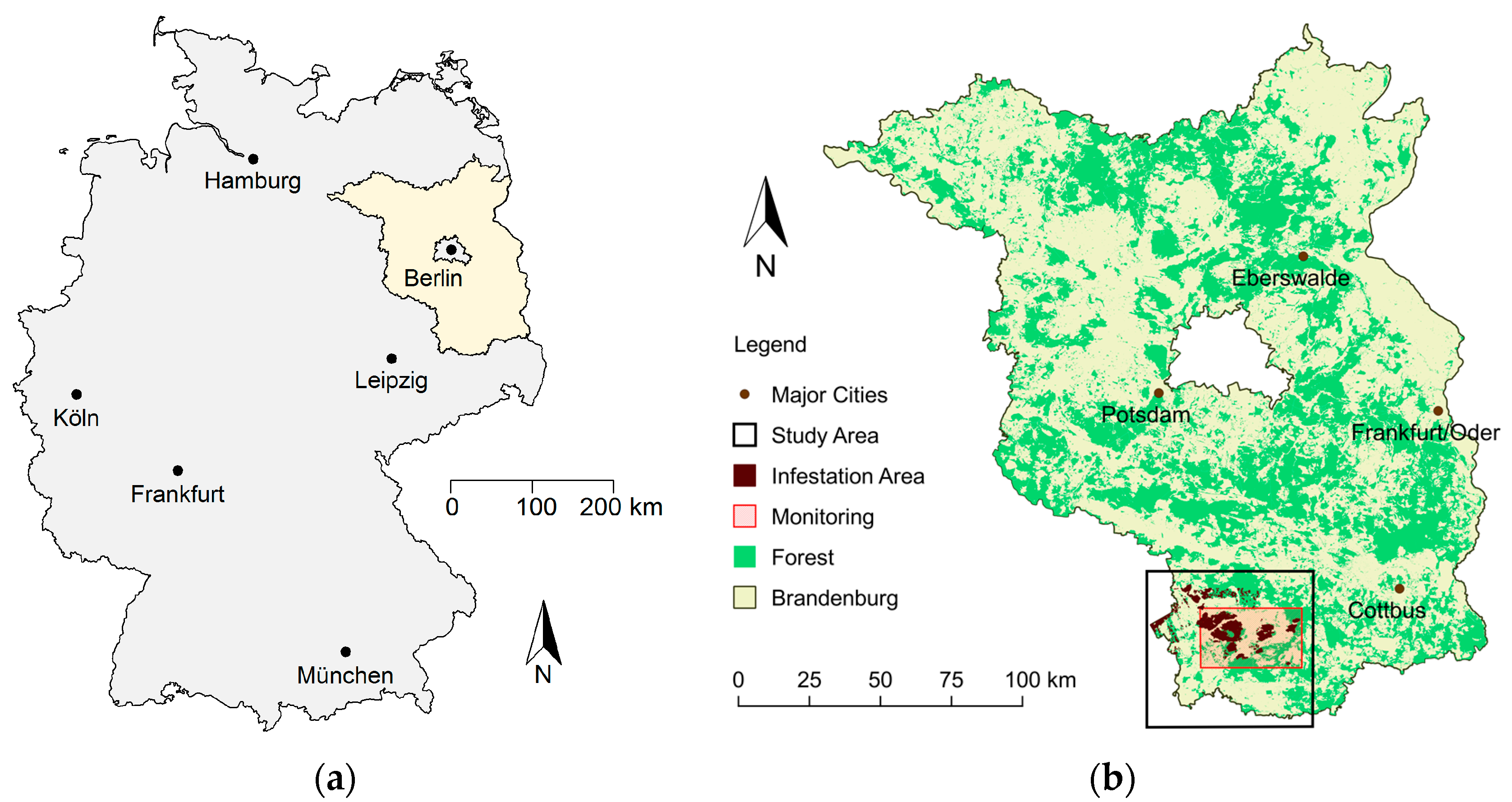
The forests in the Northeast German lowlands have suffered for many decades from frequent mass outbreaks of phytophagous insects. The German state of Brandenburg (see Figure 1) is a representative example of the environmental conditions and the challenges to forest management and protection that exist throughout this region. Scots pine (Pinus sylvestris L.) is the dominant tree species in this state accounting for more than 75% of the forested area. The climatic and pedologic characteristics of the area further aggravate the risks for mass propagations of forest pests associated with the widespread even-aged monocultures. Several remedial activities such as species diversification and improvement of structural diversity have partly begun to relieve the situation [1]. However, a large share of forests still shows a high vulnerability that requires adequate systems to monitor and counteract potentially harmful insect species. Therefore, the central tasks of the forest protection service of the Brandenburg forestry state agency are to determine pest densities, to detect the beginning of gradations, to give a precise forecast of feeding damages, and to prevent total defoliation and forest decline by applying insecticides. To further optimize monitoring and preventive measures, a thorough understanding is needed of the biological and ecological characteristics of the relevant species and of their possible reaction to the processes in the ecosystems caused by global and regional climate change [2,3].

Climate change can aggravate the damages to forest trees by a number of different but interdependent processes [4]. On a general level, it increases the total area that is accessible for potentially harmful species by “unlocking” regions that were formerly too cold or too moist [5]. Ecosystem balances, thresholds, and control cycles exerted by predators and parasites may change as a result of species-specific differences in reaction to climatic changes. Host defense mechanisms may become less active or potent due to the increasing stress for the trees resulting from the expected longer drought periods and more frequent heat waves [3,6]. The shift in habitat traits associated with climate change will also increase the risk of damages to the forest stands brought about by invasive species or species that have not been conspicuous so far [7].

Many important Scots pine pest species have been proven to prefer warm and dry summer months [4,8]. The European pine moth (Dendrolimus pini L.) and the nun moth (Lymantria monacha L.), for example, both benefit from climatic changes towards higher temperatures and less precipitation in summer as expected in regional studies [9,10]. The pine processionary moth (Thaumetopoea pytiocampa D. and S.) and the oak processionary moth (Thaumetopoea processionea L.) are other regional examples of how insect species may take advantage of favorable conditions [11,12]. A direct dependency on temperature influences the phenology of the Common pine sawfly (Diprion pini L.). 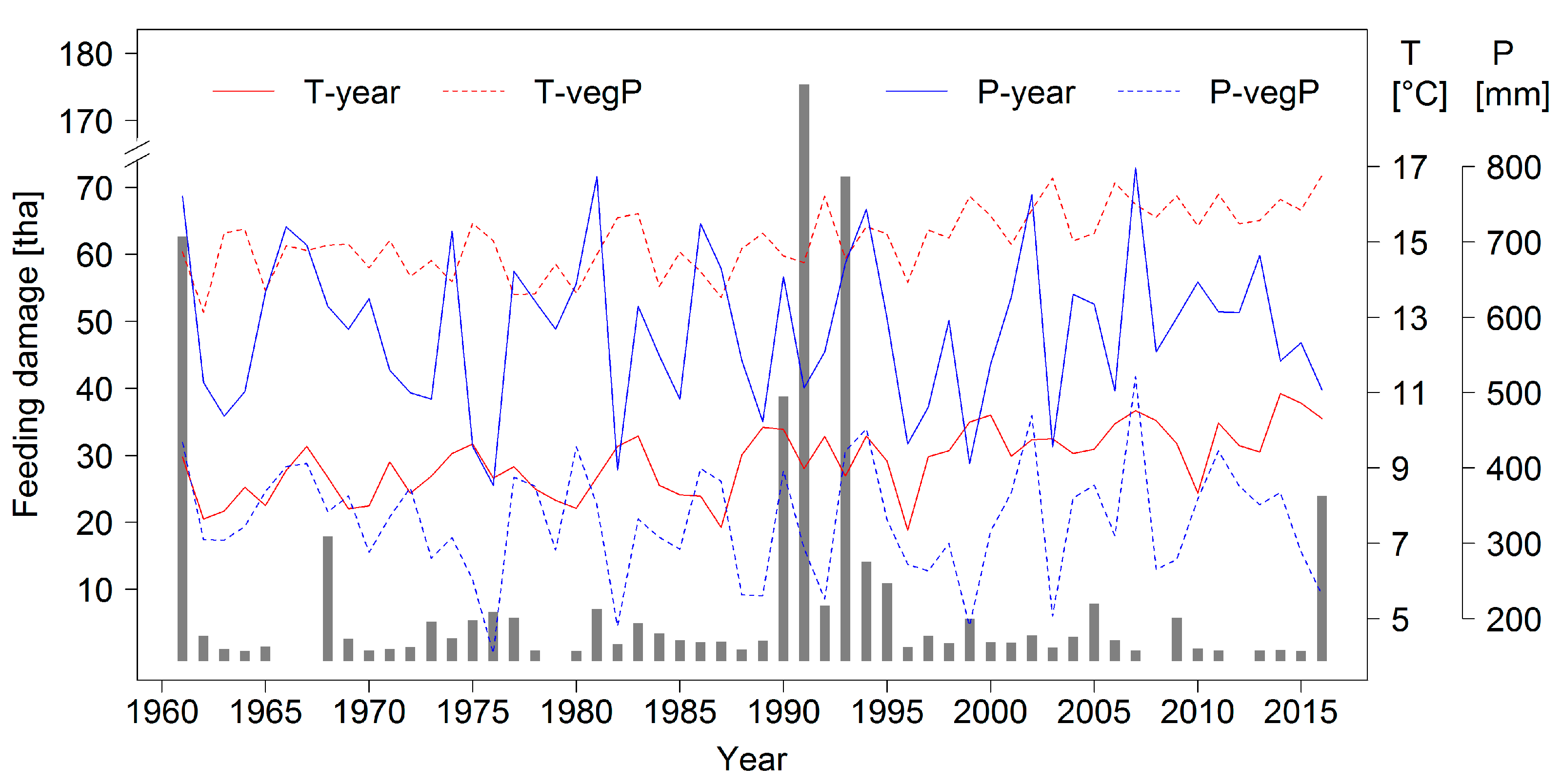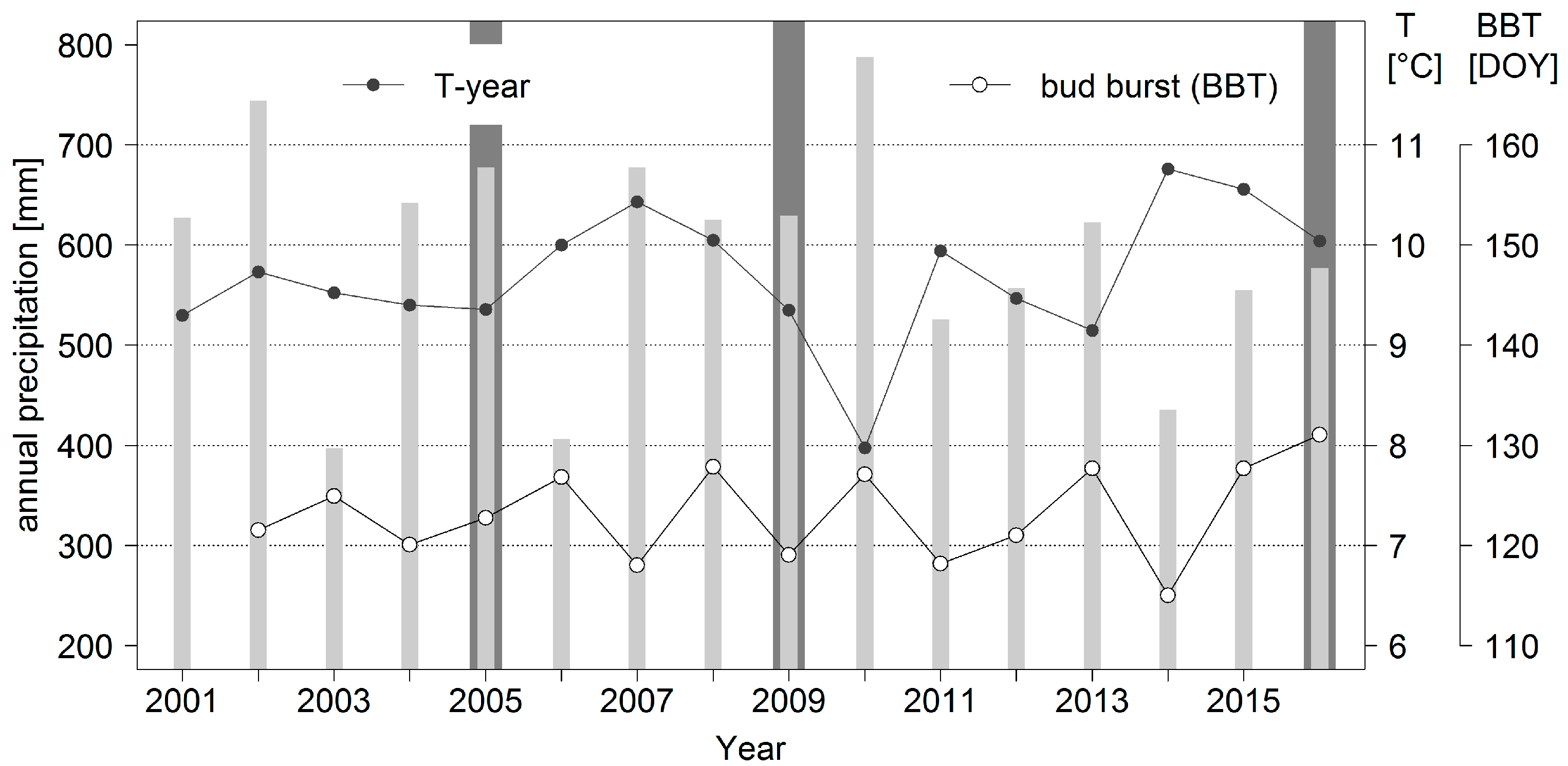Its life cycle can change from the usual univoltine pattern to bivoltine progressions as a consequence of unusually warm and dry periods [13,14]. A higher frequency in mass outbreaks and larger defoliations caused by this species may therefore be expected as a result of climate change. A time series of forest area damaged by heavy D. pini feeding is presented in Figure 2 together with annual temperature and precipitation data for the Brandenburg capital city of Potsdam to further characterize the study region.

The data presented in Figure 2 have been collected for many decades by means of a standardized forest protection monitoring and report system that covers basically the complete forest area of the state (approximately one million hectares). Foresters in the field provide the input data which are summarized and complemented by laboratory analyses by scientists at the Head Office of Forest Protection (see Section 1.2). All information for D. pini and other important pests is entered into data bases and could therefore be considered in this study. The general linking of data to geographic references as point coordinates, however, only started in 2001.

1.1. Biology of Diprion pini L.

The Common pine sawfly Diprion pini L. (Hymenoptera, Diprionidae) is known as a defoliating species associated with pine forests all over Europe [15]. Its basic biology and variable life cycle have been described, for instance, by Schwenke [13] and Eichhorn [16]. Mass outbreaks are usually followed by periods of low densities [17]. Population dynamics are influenced by genetic as well as environmental factors [18] and host plant effects [19]. Predators and parasitoids additionally influence the variability of D. pini abundance over the years [15]. Forests differ in their susceptibility to sawfly infestations, and outbreaks are reported to be more intense and more vigorous in pine forests on degraded soils [14,20].

Under the lowland conditions prevalent in Brandenburg, the life cycle of D. pini may frequently change from univoltine to bivoltine [16]. In the common univoltine cycle, the last-instar larvae in autumn disperse and build their cocoons within the litter or top layer of the soil close to the tree trunks [21]. In early April, the imagines appear and mate. The female lays eggs from April to May on one-year old needles of Scots pine. After about 3–4 weeks, the larvae hatch, often in several distinct periods (“flight waves”). The feeding of the first generation usually occurs during July and August and concentrates on two-year old needles. Because of the varying duration of the eonymphal diapause, development of the offspring of this first generation of the “lowland type” extends over three; that of the second generation (autumn-generation, egg deposition end of July to August) extends over four years [16]. Day length is a crucial factor for beginning and duration of diapause while temperature is a modifying factor [18]. Both factors are components in a complex genetic and environmental control system. The variable biology of D. pini including flexible patterns of voltinism leads to a high adaptive potential of the species over a wide climatic range [14]. Even under boreal conditions with temperatures significantly lower than in central Europe, locally adapted populations have caused large-scale defoliation in 500,000 ha of Scots pine forests in Finland [22].

Mass outbreaks of D. pini with extensive needle losses are related to bivoltine years in which a second generation of larvae hatches in the same year [13,14]. Under the influence of longer warm and dry periods, the last instar of the first-generation larvae may complete their development earlier. In this case, the larvae spin their cocoons in the pine crowns around the beginning of July and a second generation of imagines appears shortly afterwards to mate and deposit their eggs. The second-generation larvae hatch around the end of July [16]. While first-generation larvae prefer needles from the previous year, the second generation often feeds predominantly on needles developed in the same year. This can lead to total defoliation, including even the regeneration layer. Population density can multiply from first to second generation by as much as one hundred. In practice, the feeding of the first generation is usually hardly noticed by foresters and the appearance of the much larger numbers of second-generation larvae is often perceived to be utterly surprising. Thus, the identification of the infestation areas and the timely implementation of counteracting measures are, in most cases, very difficult [21,23]. The collapse of D. pini mass outbreaks is induced by a change in the emergence pattern (transition from bi- to univoltinism) and promoted by malnutrition and parasites, especially parasitoids effective in the egg and cocoon phase [15,16].

Since D. pini larvae usually do not destroy the buds of their host trees, many trees may recover quite rapidly even from heavy needle losses. Previous investigations in Brandenburg during the last 25 years have shown that Scots pine trees have a good chance to regenerate within 2 to 4 years if the remaining needle mass after caterpillar feeding is at least 10%. Below this threshold, however, the mortality rate of the trees goes up to 60–100% [24]. Climatic conditions in the two years after defoliation play a crucial role in successful recovery—the stronger the climatic stress factors that affect the damaged trees, the higher potential losses will be [5]. Additionally, warm and dry conditions in subsequent years promote the development of secondary pests such as bark beetles that can further aggravate the situation and eventually lead to tree mortality [7,25]. As these climatic factors are likely to become more frequent in the coming decades, effective monitoring and risk management will be even more important in the future [5,26].

1.2. Risk Management

Monitoring procedures and decisions about control measurements in the pine forests of Brandenburg are the result of long-term experiences with heavy or total needle loss caused by defoliating insects. The basic spatial reference unit for forest management and protection in Germany is the “forest compartment” which in the study area has a median size of 27 (0.4–230) hectares. According to the range of species involved, risk management traditionally focuses on a group of species comprising European pine moth (Dendrolimus pini L.), nun moth (Lymantria monacha L.), pine looper (Bupalus piniaria L.), pine beauty (Panolis flammea D. and S.), and pine sawflies (Diprion pini L., D. similis L., Gilpinia frutetorum Fabr.). While the first four species exhibit a rather predictable life cycle and mass outbreak pattern, the Common pine sawfly (D. pini) poses specific challenges to monitoring and control algorithms because of the variable, “surprising” biology of the species on the one side and the high damage potential for pine stands through feeding of the second generation on the other side [16]. Consequently, effective monitoring methods and timely, realistic prognoses are particularly essential for successful risk management of D. pini. Reflecting regional experience and numerous studies, the overall aim is to prevent needle loss of more than 90% [24,27].

To supervise the first generation of sawflies, the following monitoring steps are applied:

• December to January: winter soil investigation, estimation of the number of cocoons per m², determination of vitality (parasitization) and development stage of nymphs (diapausing larvae) in the laboratory;
• After hatching and egg deposition: estimation of number of eggs per crown by an established sampling scheme (3–5 sample trees felled in affected stands), determination of the degree of egg parasitization.

The second generation of sawflies is monitored, if necessary, as follows:

• Beginning of July: felling of sample trees to check if the larvae have reached the last instar (length ≥2.2 cm; head capsule width 1.8–2.2 mm);
• Middle of July: estimation of the number of cocoons per crown, determination of vitality (parasitization) of the nymphs in the laboratory;
• End of July/beginning of August after hatching and egg deposition: estimation of the number of eggs per crown, determination of the degree of egg parasitization.

The subsequent damage scenarios are based on the monitoring data obtained by the procedures listed above. To delimit the area of potential application of insecticides as exactly as possible, the necessary data are gathered at a spatial resolution of about 25–50 hectares. For each generation (spring and summer), the amount of eggs is compared to species-specific critical threshold values depending on age, site index of the respective stand and mean foliage intactness. Abundances of D. pini above these critical values will most probably lead to complete defoliation according to current scientific and experimental knowledge. The actual risk for a forest stand to experience total defoliation is expressed in relative threshold numbers (TN). TN ≥1 reads as a safe prognosis of total needle loss.

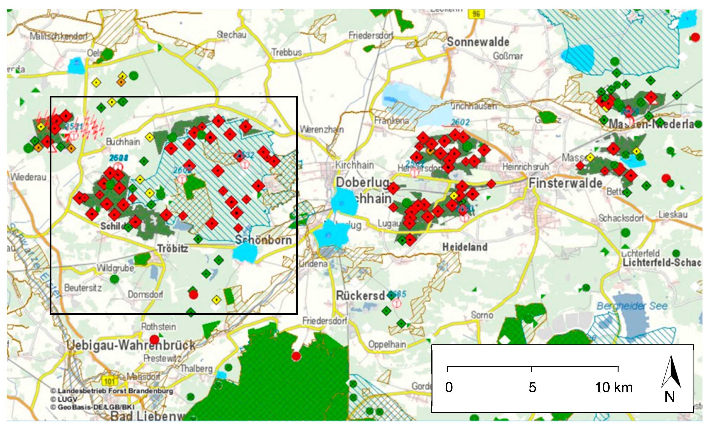
Identification and delimitation of infested areas and feeding intensities are supported by satellite data acquired by the RapidEye sensor (BlackBridge/Planet Labs Inc., San Francisco, CA, USA [28]). The derived images show the spatial differences in foliage productivity (and thus of the existing needle mass) based on the NDVI (Normalized Difference Vegetation Index) at a resolution of 5–6 m. All information, including on-the-ground assessments of feeding damage and the development stage of the responsible species, is combined and analyzed by means of geographical information systems. Since 2015, the forest administration in Brandenburg uses a special “Web Office” portal for data input by the foresters. The application allows for the documentation of estimated threshold numbers (Figure 3) and finally the supervision during the whole administrative and technological process [26].

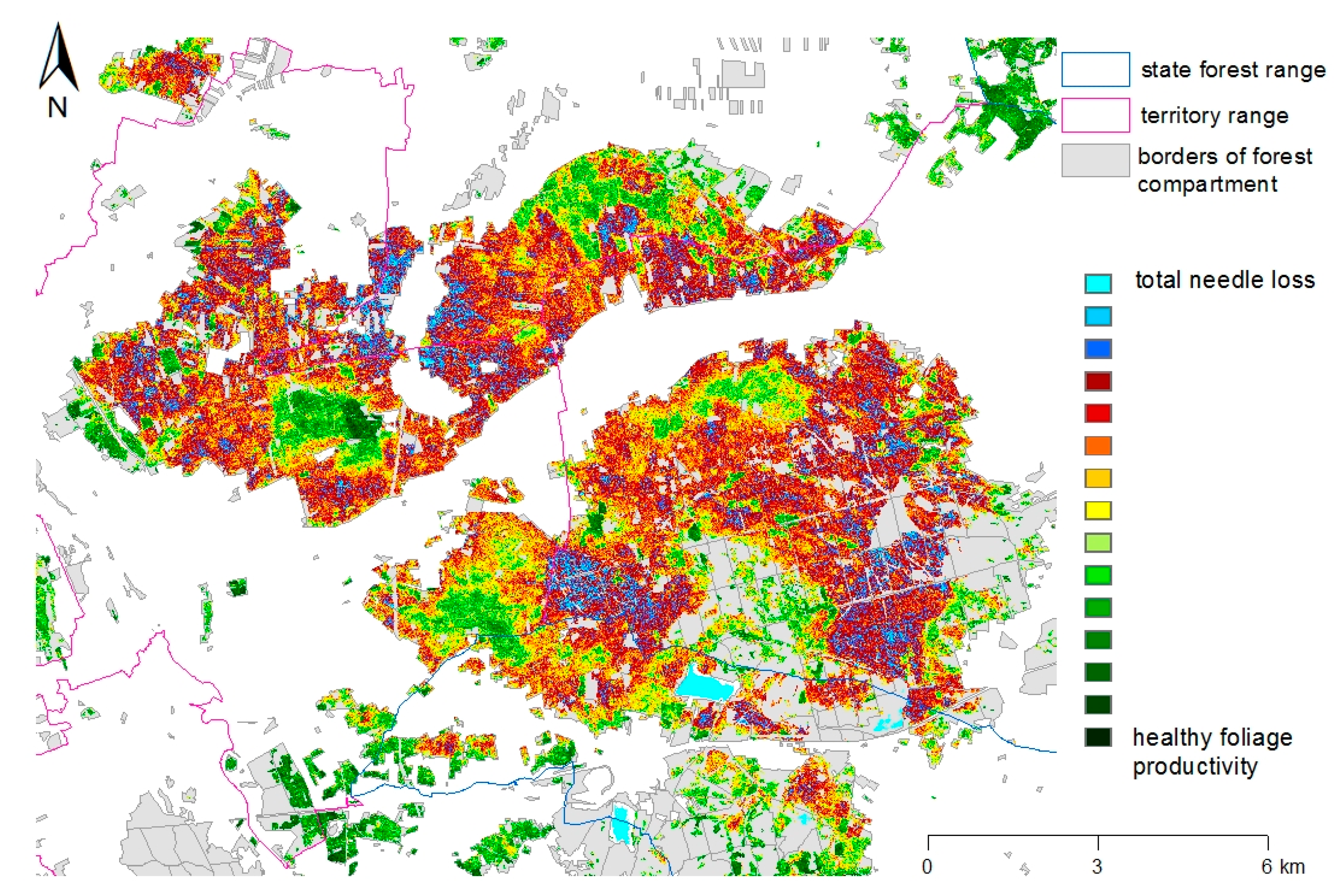
In August 2016, the preceding monitoring steps projected total needle loss for an area of nearly 5000 ha in the study area. From the end of August to the beginning of September, a contact insecticide was applied on 2800 ha of Scots pine forests. In late autumn, the high quality of the system could be verified by comparing the damages in treated and untreated forest compartments (see Section 1.2) on the basis of new RapidEye data taken after the feeding period (Figure 4). Eventually, a total of approximately 1300 ha of pine forests in the region were classified by the satellite data as completely defoliated which means that more than 90% of the needle mass had been lost [23]. The vast majority of this area belongs to nature reserves or is situated close to roads and settlements and was therefore excluded from insecticide treatments. The remaining potentially threatened area had been successfully protected.

1.3. Focus of the Study

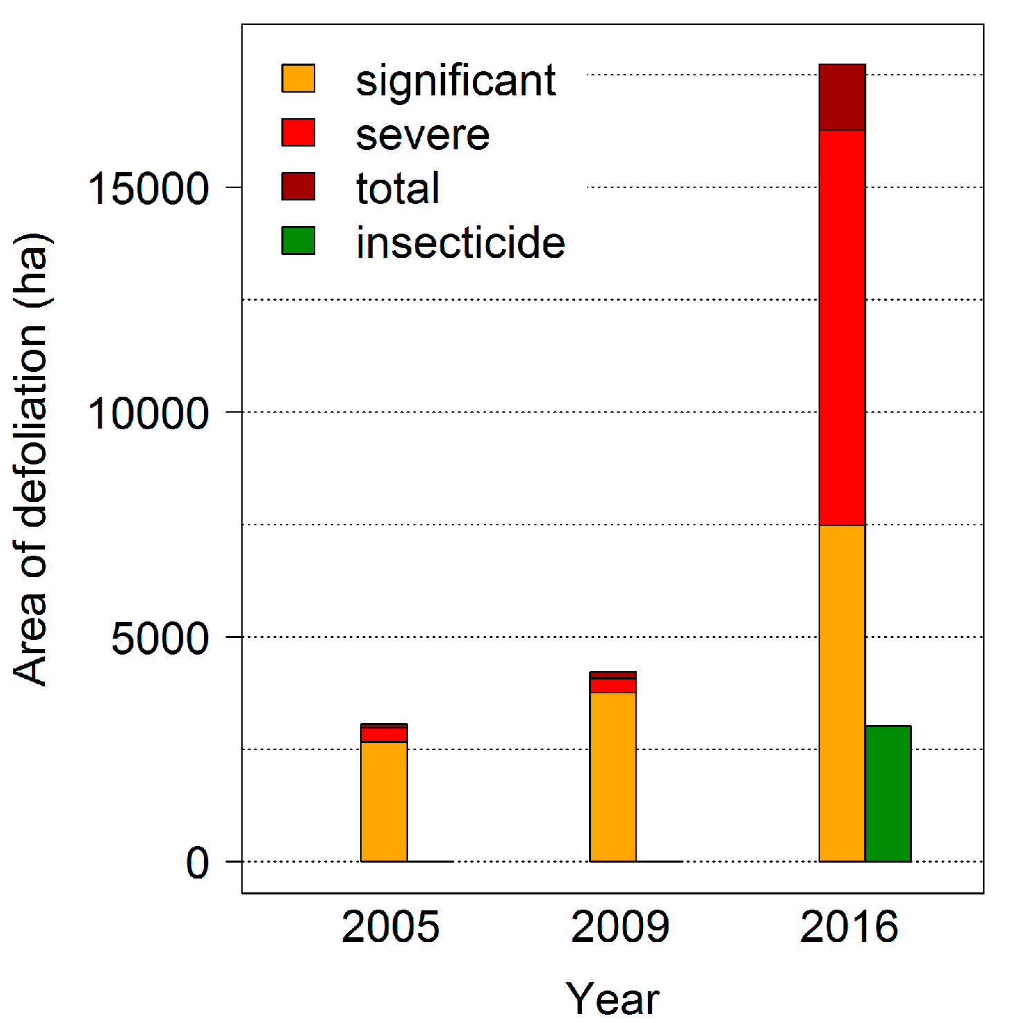
The last mass outbreaks of the D. pini in Brandenburg were observed in 2005, 2009 and 2016 with intensive feeding damages by a second larvae generation during late summer to the beginning of October (Figure 5). In 2016, almost 50,000 ha of Scots pine forest were affected; both the infestation area and the feeding intensity reached extremely large dimensions, verifying the predictions of larger outbreaks in the future. In the study area, a total of 23,000 ha—including areas where insecticides were applied—was damaged by significant (31–50% needle loss), severe (50–90% needle loss) and total (less than 10% of foliage remaining) defoliation (Figure 5).

The immediate challenge in a case like this is to carry out a comprehensive and successful monitoring at the onset of the second generation, or even earlier, in order to realistically assess the scale and distribution of the potential defoliation. The time period for the required monitoring is rather short due to the rapid development cycle of the species. This period is also limiting the time to complete the administrative process necessary for preparing insecticide application by helicopters. Therefore, a central task to promote successful risk management in the future is to identify the factors that provoke the change from univoltinism to bivoltinism in the insect populations. Finding these “triggers” for potential mass outbreaks will provide a more precise and reliable basis for preparing control measurements and to promote potential applications of insecticides.

The objective of this paper is to provide new insights into the links between climatic factors and the course of intra-annual development of D. pini in the state of Brandenburg as an example for similar conditions in lowland, semiarid regions in Central and Eastern Europe. We outline the life cycle of the species and summarize the current monitoring procedures and explanatory information used by the forest protection service in Brandenburg to predict and counteract D. pini mass outbreaks. Finally, we will discuss the consequences of our findings and propose adjustments in the current forest protection routines to limit future damages. At the core of our investigations is the search for statistical patterns in climatic conditions that provoke mass outbreaks. In relation to these analyses, we hypothesize that

(1)

the relations of D. pini abundance to climatic factors cannot be fixed to average, general conditions at an annual scale but are rather influenced by relatively short periods;

(2)

flexible floating windows attached to plausible phenological dates will prove more useful as explaining variables than periods related to fixed calendar dates;

(3)

there are no single predominant variables that control population dynamics. Instead, a complex interaction of climatic factors is responsible for local and temporal variance of mass outbreaks.

2. Materials and Methods

2.1. General Approach

It has been shown that the population dynamics of D. pini are a result of many factors ranging from site characteristics and tree disposition to climatic variables and parasitism [19]. Monitoring and risk management of the species depends on information of where and when mass outbreaks are likely to occur. In this study, we focus on climatic factors which can help to explain both dimensions by analyzing their spatial and temporal variability within a specific region and time frame. In order to identify the climatic conditions that are most likely to promote the appearance of a second generation within one year, we apply the “Random Forest” approach for classification [29]. The implemented variable importance measure of this method allows us to determine the most important climate variables and timescales related to the observed mass outbreaks of D. pini. The analyzed time scales are adapted to the start of the growing season of the host species Scots pine modeled according to Menzel [30].

2.2. Temporal Scale

The life cycle of D. pini consists of intervals which are determined in their onset and termination by “switches” or triggers linked to climatic key factors. Although there are general reference ranges for the timing of these steps that are usually referred to [16], the exact dates vary from year to year in response to the respective environmental conditions. At the annual level, there is a notable lack of synchrony between time series of basic climate data and outbreak years (Figure 2). This apparent independence is also obvious at the smaller scale in the study area (Figure 6).

Detailed models that intend to identify the factors leading to mass outbreaks have to consider this missing coherence between annual data and feeding events (Figure 6) and reflect the dependence of D. pini on fine-scale climatic triggers. As a consequence, our investigations include intervals attached to varying phenological dates rather than to fixed DOYs (Day Of Year) to estimate the beginning or end of the life stages of the respective populations. Additionally, we tested conventional climatic windows such as annual and monthly aggregates and averages for their influence on outbreak patterns in order to cover a wide range of possible correlations.

2.3. Climate Data

The climatic conditions of the individual forest compartments are represented by regionalized daily climate data [31] based on measurements of the German Meteorological Service (DWD). According to reference studies by other authors [16,20] and on the data available for the study region, we focused on the following range of climatic factors:

• Temperature: daily mean, daily minimum, daily maximum of air temperature at 2 m above ground (°C)
• Precipitation: daily sum (mm)
• Evapotranspiration: daily sum (mm) modelled according to Penman-Monteith [32]

The following temporal intervals of the climatic factors were analyzed:

• Annual, growing season (April to September) and monthly composites
• Aggregates of days in periods of at least 7 days (1–8 weeks)
• Composites and aggregates from the year prior to the actual feeding event

Based on the close temporal synchrony between host development and insect phenology [33], we used day of bud burst (BBT) as estimated by the phenological model developed by Menzel [30] as an indicator of the specific climatic conditions in a given year. This model is a function of the daily mean temperature with specific threshold values of both warm and chill days and showed a good match with observed bud burst in forest stands in Brandenburg. Annual dates of BBT usually vary between DOY 118 and 128 which translates to April 28 and May 8, respectively. This period corresponds to the interval when D. pini imagines swarm and mate [16]. A second period subjected to detailed analysis covers the time of pupation and—in bivoltine years—hatching of imagines at the end of July. It was dated as DOY of bud burst plus 90 days (BBT + 90) which translates to a range between July 27 and August 6. The resulting DOYs and the connected periods were abbreviated as FLY factors because they determine whether there will be a second generation in the same year. In relation to the phenological dates of BBT and FLY, we created factors with a length of at least one week covering all possible combinations of weeks before and after the respective date, starting 28 days before and ending 28 days after BBT and FLY (see Figure 7 for a visual example).

For a general description of the intra-annual variation of the climatic conditions, we also included four aridity/humidity indices. These indices differ mainly in how they select and weight the importance of their input variables (daily temperature, precipitation, and evapotranspiration data):

• Climatic water balance (expressed by the difference between annual precipitation and annual potential evapotranspiration according to DWD data)
• Köppen index (1923; see [34])
• Seljaninov coefficient (1937, see [10])
• Thornthwaite index [35]

The statistical analyses included sum values, mean values, and the respective standard deviations of all parameters. The resulting data set consisted of 1142 variables of climate composites and aggregates based on a regionalization process which provided individual estimates for the center points of all investigated forest compartments.

2.4. Determination of Variable Importance

In order to determine the most important climate variables in relation to the successful development of mass outbreaks by D. pini, we applied the “Random Forest” (RF) approach introduced by Breiman [29]. This classification approach constructs a forest of uncorrelated decision trees by a randomly selected subset of variables for each node of a tree. As a central advantage, the RF can handle high numbers of variables and does not tend to over-fitting [29]. Furthermore, it provides a measure of the variable importance (e.g., [36]).

The RF was applied on climate data of all those forest compartments that have been affected by defoliation since 2002. Therefore, the measures of the variable importance refer to the differences between individual years. They do not reflect the spatial distribution of defoliation possibly corresponding to the favorable feeding conditions of the forest. In total, we considered 534 forest compartments in which 695 defoliation events had been observed.

The RF has been implemented in the statistic software “R” [37] using the ’randomForest’ package [38]. We used the ’tuneRF’ function in order to find the optimal number of predictors for the construction of the decision trees. Based on a 10-fold cross-validation and a default number of 1000 decision trees, the variables were ordered by decreasing importance according to the average of the “mean decrease Gini”. This parameter is considered to be a more robust measure of variable importance compared to the “mean decrease accuracy” measure available in RF methodology [39]. As a reaction to the imbalance of class frequencies of approximately 1:10 with the majority of non-defoliation observations considering the years 2002 to 2016, the training set for the RF was down-sampled to a 1:1 ratio as suggested by Chen et al. [40]. Consequently, the training set for each cross-validation step contained 90% of the defoliation observations and the same number of randomly chosen non-defoliation observations. After each cross-validation step, a prediction was made for the remaining 10% of the data set (type = “response”) by the previously trained RF.

The Random Forest approach produces an ordered list of climatic variables that contribute to the statistical separation between defoliation and non-defoliation by D. pini. In the next step, we selected four of the top-ranked variables (“top four” trigger variables) from this list for the differentiation of the individual years in order to identify specific climatic conditions of the mass outbreak years of D. pini. We analyzed the distribution of these top four variables by means of box–whisker plots showing the variance and the mean range of the variables in outbreak years. The total range of the values of the “top four” in the period 2002–2016 was then stratified into five classes from 1 (inconspicuous) to 5 (most severe, i.e., most favorable for an outbreak) according to the distribution of the respective variable during mass outbreaks: If a variable showed predominantly low values in outbreak years, the highest rank (class 5) was associated with low values; if high values were associated with outbreaks, then class 5 was assigned to forest compartments exhibiting the highest values of the respective variable. In the last step, we merged the four selected climatic factors by adding the class numbers of each variable into a pooled level variable “risk class” that we plotted on a map of the study area. This “risk class” may consequently fall into a range between 4 (least conspicuous) to 20 (most probable combination for massive feeding). Using this algorithm, we produced maps of all years that show the sum of the classifications by a five-class color scale which can be utilized as an initial tool for an enhanced monitoring system.

3. Results

The RF approach showed good performance in realizing an area under the receiver operating characteristic curve (AUC) of 0.97 [41]. Based on the test data sets of the 10-fold cross-validation, we achieved a true positive rate (TPR) of 95% (non-defoliation compartments) and a true negative rate (TNR) of 98% (defoliation compartments).

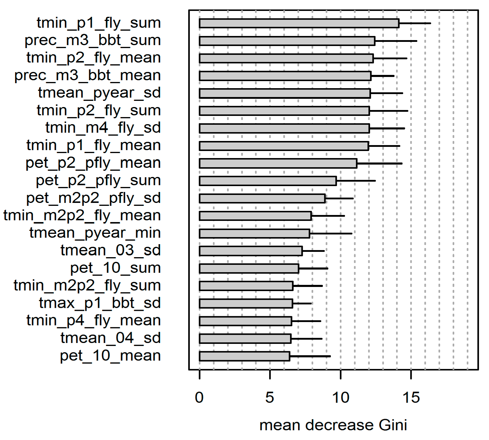
The 20 most important variables of the performed RF classification are shown in Figure 8. A description of the variable name abbreviations is given in

Table 1. Description of the top 20 explanatory climate variables.

Acronym	Explanation
tmin_p1_fly_sum	sum of daily minimum temp. in first week after FLY 1
prec_m3_bbt_sum	sum of prec. in three weeks before BBT
tmin_p2_fly_mean	mean of daily minimum temp. in two weeks after FLY
prec_m3_bbt_mean	mean of daily prec. in three weeks before BBT
tmean_pyear_sd	standard deviation of daily mean temp. of previous year
tmin_p2_fly_sum	sum of daily minimum temp. in two weeks after FLY
tmin_m4_fly_sd	stand. dev. of daily minimum temp. in four weeks before FLY
tmin_p1_fly_mean	mean of daily minimum temp. in one week after FLY
pet_p2_pfly_mean	mean PET in two weeks after FLY of the previous year
pet_p2_pfly_sum	sum of PET in two weeks after FLY of the previous year
pet_m2p2_pfly_sd	stand. dev. of PET in two weeks before, two after FLY of the previous year
tmin_m2p2_fly_mean	mean minimum temp. in two weeks before, two after FLY
tmean_pyear_min	minimum of daily mean temp. in previous year
tmean_03_sd	stand. dev. of daily mean temp. in March
pet_10_sum	sum of daily PET in October
tmin_m2p2_fly_sum	sum of minimum temp. in two weeks before, two after FLY
tmax_p1_bbt_sd	stand. dev. of maximum daily temp. in one week after BBT
tmin_p4_fly_mean	mean of daily minimum temp. in four weeks after FLY
tmean_04_sd	stand. dev. of daily mean temp. in April
pet_10_mean	mean of daily PET in October

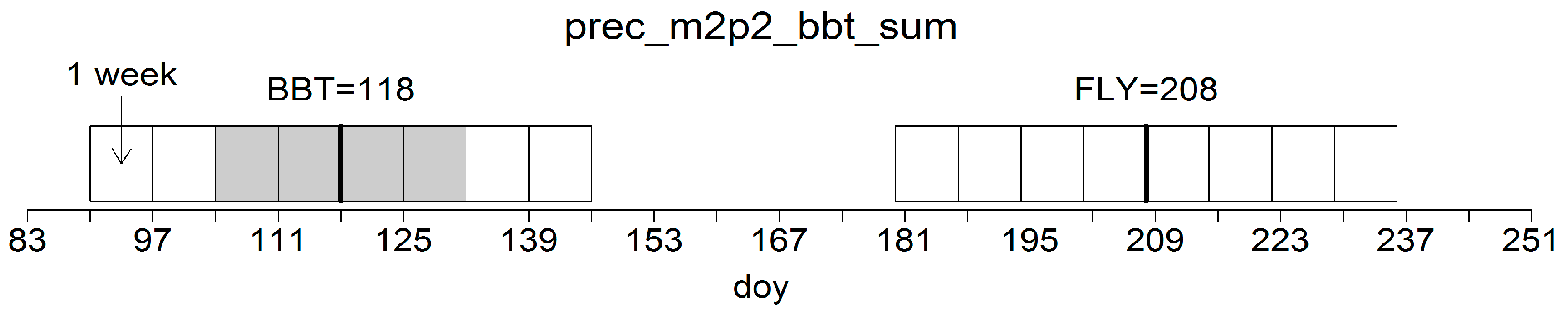
¹ temp.: temperature, prec.: precipitation, PET: potential evapotranspiration; for FLY and BBT, see text above table and Figure 7.

. In the variable coding, the first character string defines the basic climate data and the last character string represents the applied metric (sum, mean, and standard deviation). The character string in-between describes the temporal reference which is defined either by the phenological dates BBT and FLY (Figure 7), the complete year or by single months as indicated by the numbers 01 to 12. Previous-year climatic conditions are labelled with “p”, e.g., “pyear” or “pfly”.

We used the average of the “mean decrease Gini” measure (Figure 8) to obtain nine central variables exceeding the value of 10 and producing a distinct decrease of the importance measure for the following variables. The standard deviation showed a comparable magnitude for all variables as a result of the 10-fold cross-validation process and the respective variation of the training data. Note that various variables differed in the particular time window (e.g., p1_fly vs. p2_fly) or in the statistical parameter (e.g., sum vs. mean) only and were, thus, strongly correlated. The correlation matrix of the top 20 explanatory variables can be found in the supplementary material (Figure S1).

The arity/humidity indices did not show up in the top 20 of most important variables. The majority of variables were related to the phenological dates of BBT and FLY. The calculation of either the sum or the mean of the particular variables did not affect the variable importance and both metrics showed a comparable magnitude of the “mean decrease Gini” measure for equal basic data and temporal scale (Figure 8).

In selecting the “best” trigger variables, we have considered both the ranking of the variable importance and the diversity of the information provided by the climate variables. We neglected variables of equal core data within similar time windows (highly correlated variables; see Figure S1). 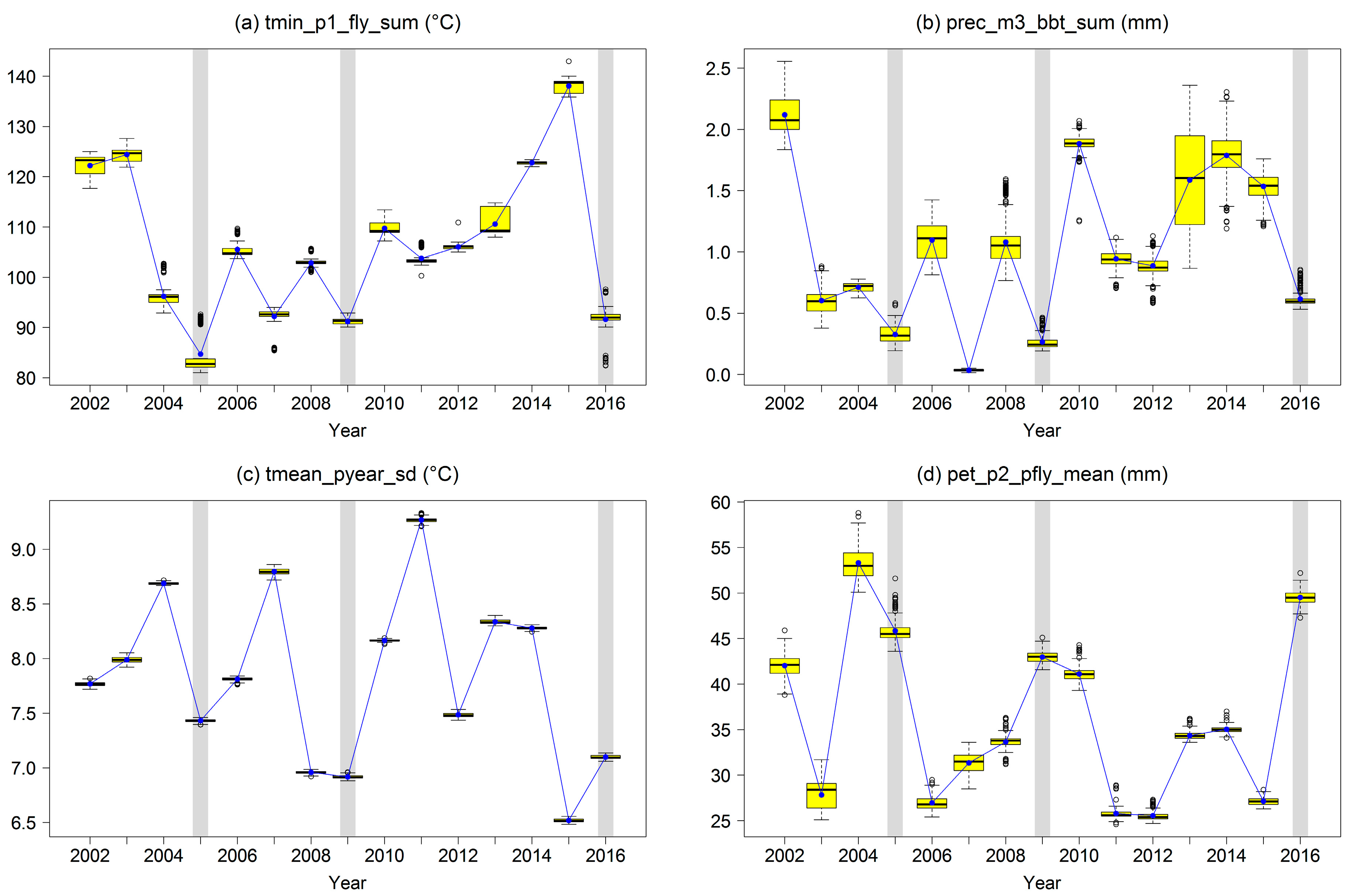With respect to the distinction of the basic climate data and the particular timeframe accessed, we could identify four variables exhibiting the highest explanatory feedback on mass outbreak years of D. pini:

(1)

tmin_p1_fly_sum: sum of daily minimum temperature over 7 days after FLY

(2)

prec_m3_bbt_sum: sum of precipitation over 3 weeks prior to BBT

(3)

tmean_pyear_sd: standard deviation of daily mean temperature of the previous year

(4)

pet_p2_pfly_mean: mean of daily “pet” over 2 weeks after FLY of the previous year

These top four trigger variables showed a clear differentiation for outbreak years by generally lower or higher values compared with the other years (Figure 9). For outbreak years, low minimum temperature at FLY and low precipitation at BBT can be observed. The particular previous years are characterized by low standard deviation of the mean temperature and high potential evapotranspiration at FLY. The correlations between the top four trigger variables were relatively low (Spearman’s rank correlation coefficient below 0.44) with the exception of tmin_p1_fly_sum and prec_m3_bbt_sum showing a rank correlation of 0.74 (Figure S1).

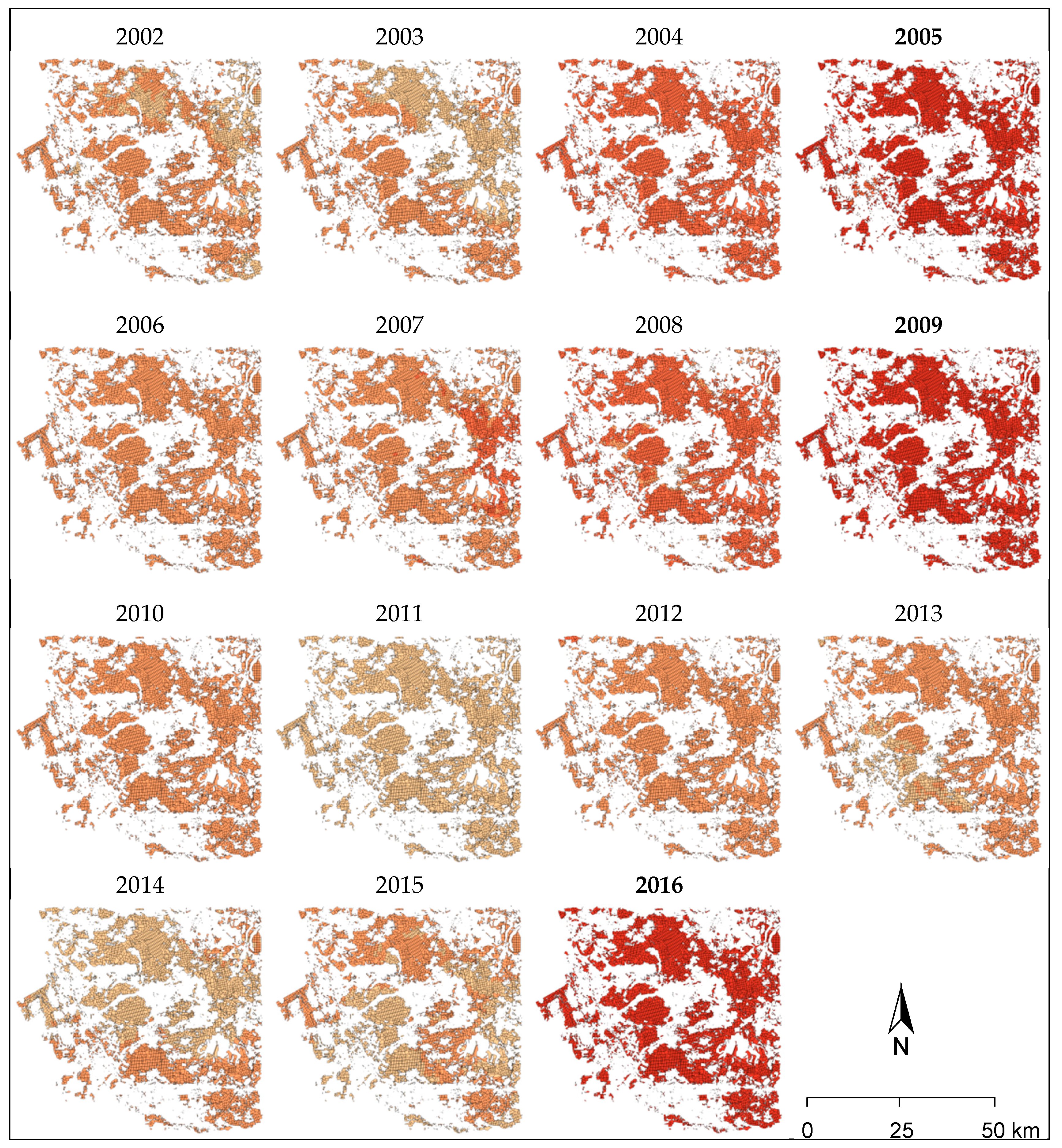
The pooled level variable “risk class” translates the combined impact of the top four trigger variables into a categorical variable. Figure 10 shows the spatial distribution of the “risk class” within the study area and for all individual years. The years of mass outbreaks of D. pini (2005, 2009, and 2016) were always connected to the highest classes across all forest compartments as indicated by dark red coloring. The years prior to the mass outbreaks in 2005 and 2009 showed the second highest class assignments. All other years had lower class assignments and a higher variability within the study area.

4. Discussion

The susceptibility of forests to sawfly infestations depends on a wide range of different factors. It has been shown, for instance, that mass outbreaks are more severe in pine forests on poor or degraded soils [19,20,22] and on dry sites with deep ground water [14]. Composition and activity of natural enemies also strongly depend on the particular habitat conditions in a forest [42]. Rich and diverse forest structures, as associated with mixed, multi-age stands, are assumed to support a more stable and more diverse community of antagonists that can limit possible mass outbreaks [43]. The impact of cocoon predators on sawfly densities can vary in forests of different fertility [44]. In contrast, little is known about a possible link between forest structure and parasitism of pine sawfly larvae in the cocoon phase [15]. However, natural enemies such as parasitoids effectively influence an outbreak only after its culmination has already occurred, so they have no real relevance for determining key factors for voltinism change. The time lag between mass propagations and antagonists has been confirmed by analyses in Brandenburg in late summer 2016 that found nearly 100% vitality in D. pini eggs produced during an active outbreak [23]. Host needle quality is another important factor affecting egg numbers, hatching rates, and success of larval development of the pine sawfly [14,19,45]. Out of this large range of possible influences, we concentrated on the climatic factors that are most likely to control inter-annual variation in population density and the occurrence of mass outbreaks [4]. Factors related to tree [22], stand [46], and soil characteristics or the abundance of antagonists were seen as ceteris paribus conditions that we neglected in our analyses.

While the individual climatic factors were chosen according to their acknowledged impact on population dynamics, we chose the analyzed temporal windows in two ways: (i) as composites for conventional, fixed-position intervals (months, growing seasons and years); and (ii) as composites of flexible, “floating” windows attached to basic phenological dates depending on the specific annual climate. The causal bias in data selection effective in the latter group is thus compensated by the neutral background of the first group. Except for the partial attachment to flexible dates, the developed trigger variables were derived from complex statistical procedures which do not take into account any possible cause–effect relationships. To assess the quality of our approach, however, the evolved parameters that influence D. pini population dynamics should be evaluated both in their statistical validity and in their biological plausibility as well.

The chosen approach to determine the critical parameters that are most likely associated with conditions leading to mass outbreaks relies heavily on intricate statistical techniques and a detailed, multi-facetted database. In any discussion of the validity of our results, we have to acknowledge this methodological background and the complex nature of the applied ensemble-learning method for classification. This method searches for an optimal feature combination to divide a given data set into its (here) two categories (defoliated vs. non-defoliated forest compartments). Therefore, the proposed variable importance and the suggested top four trigger variables mainly represent the optimal split points of our specific training data rather than any deterministic cause–effect chains of dependence.

The mean variable importance, however, stayed stable within the cross-validation process (including variations of the number of decision trees used in RF and the initial random seed number) but may vary if the data base changes, e.g., by increasing the number of observations of the majority class for training. For example, when applying the whole data set of the observation area (3864 forest compartments by 15 years and a respective class frequency of 1:78) the best split points were found for standard deviation parameters and precipitation variables (data not shown). We suppose that these climate variables are more likely to account for spatial patterns of the study area. Furthermore, we considered highly correlated predictors in our analysis which is why the importance measure may be very sensitive to changes in the data base. Genuer et al., however, showed that even if the value of the importance measure decreased when adding highly correlated variables to the training data of their study, true variables could not be confused with noise variables [36]. In fact, the “top four” trigger variables were selected from different core data (minimum temperature, precipitation, mean temperature and potential evapotranspiration) and provided different information about the climatic conditions. The strong correlation (Spearman’s rank correlation coefficient of 0.74) between minimum temperatures around FLY (tmin_p1_fly_sum) and rainfall prior BBT (prec_m3_bbt_sum) is considered to be accidental. Due to the independence of the distribution of precipitation from the phenological year (determined as a function of the temperature), we argue that both variables impact different stages of the development of D. pini and should therefore be considered individually in the analysis.

We have applied several data subsets and RF specifications, e.g., balancing and weighting practices [40] that are not presented here. Neither can we discuss the issue of variable importance stability in detail [36,47,48]. We rather present a study focusing on the application of the RF approach in the light of forest protection issues. In fact, the top-ranked variables showed a clear differentiation of the years (Figure 9), in particular if all four parameters are combined (Figure 10). Thus, we argue that the presented top four trigger variables are closely linked to critical stages in the development of D. pini. Unfortunately, we were not able to test this hypothesis against the whole time series of historical observations of defoliation (Figure 2) because of flaws in data quality and in particular the lack of spatial references for these data. The only independent data available are from an area in the North of Brandenburg where a mass outbreak of D. pini occurred in 2005. The classification of the individual years following the same procedure as shown in Figure 10 yielded comparable results with most favorable climate conditions for outbreaks of D. pini in 2005, 2009, and 2016 (data not shown). On the one hand, we can confirm the correct classification of the year 2005 by the four trigger variables. On the other hand, the four trigger variables may perfectly differentiate 2005, 2009, and 2016 from the other years in the observation period but the outbreak in the North of Brandenburg in 2005 may have been matched accidentally.

Due to the small sample size of three outbreak years in Brandenburg and the lack of independent data, we cannot prove the causal relationship between the four trigger variables and the mass outbreaks of D. pini. Consequently, further research is needed to test the validity of our findings on independent data and/or future defoliation events. A critical aspect, however, is the combined impact of climate and site effects [14] on D. pini populations. The absence of pine sawfly outbreaks in the north of Brandenburg in 2009 and 2016 might result from changes in stand structure by forest growth and management activities leading to changes in micro-climate [4,43], food quality [19,45], or the abundance of antagonists [44,46]. Based on the data available in Brandenburg from 2002 to 2016, however, we can present four climatic variables most likely related to the population dynamic of D. pini.

Although exceptionally warm and dry summers are often referred to as being beneficial for mass outbreaks [4,7,14,20], our findings show that “warmer climate” in general cannot be held accountable for increasing risks associated with D. pini. Instead, there are specific, flexible intervals of climatic factors which—in complex interaction—create favorable environmental conditions for mass outbreaks. For successful mass propagations, these climatic factors need to meet the needs of both the first- and the second-generation sawflies in their particular development stages. The attachment to floating phenological dates has proven beneficial to increase the performance of the classification: except for the standard deviation in the previous year’s temperature, all variables refer to either bud burst or to the “fly” period 90 days later (Figure 7). This may indicate a strong relationship of the development of the pest species with host physiology. For many forest insects, the hatching of the first-generation caterpillars needs to synchronize with the bud burst of the host [16,33]. Thus, it seems reasonable that the climatic conditions prior to BBT need to be favorable for egg and caterpillar development. Rainy days associated with low temperatures are obviously detrimental conditions.

The impact of the climatic conditions around FLY is probably related to both the flight conditions of the first-generation adults and the development of the second-generation eggs. In the year of the actual mass outbreak, we assume that the positive effect of relatively low temperatures after flight/mating (tmin_p1_fly_sum) reflects the susceptibility of the eggs against heat and draining. Temperatures in this period might also affect the life span of the female imagines, with lower values reducing energy consumption and thus prolonging the time for egg deposition. High potential evapotranspiration resulting from dry and/or warm climate around FLY of the previous year (pet_p2_pfly_mean) is supposed to be associated with optimal flight conditions and a maximal vitality of the larvae entering hibernation. This factor becomes effective in combination with relatively constant conditions in the previous year (tmean_pyear_sd) allowing a relatively undisturbed pre-gradation. Low precipitation in the weeks before bud burst (prec_m3_bbt_sum), i.e., in late April to early May, is often related to higher temperatures and overall favorable conditions for flight, mating, and egg deposition of the first-generation imagines. However, due to the complex biology of D. pini, including dormancy cycles, it is difficult to distinguish between climate impacts on egg, caterpillar, and adults of the various generations [18].

From an ecological point of view, the discussed relations between climate and population development cannot be seen as independent from ecosystem factors and processes beyond the individual species [44]. Climatic impacts may not only be direct but additionally affect D. pini populations indirectly via effects on host vitality including protective capacities [4]. Trees may counteract, for example, the characteristic “slicing” of the needles by the female imagines before egg deposition by resin extrusion. The amount of energy available for this reaction is dependent on the level of stress or resource depletion exerted on the tree by the climatic circumstances. Food quality is dependent on the productivity of the site, current climatic stress experienced by the trees, and other factors such as competing defoliators or past stress events. The concentrations of the physiological compounds, for example, change during needle life cycle. Kätzel and Löffler [49] found that the concentration of carbohydrates and ascorbic acid too increase from one- to two-year-old needles. Furthermore, the concentration of secondary plant compounds responsible for pest defense such as phenolic compounds is dependent on needle age as well as on past stress events and needle loss [50]. The ratio of both nutrients and response compounds in Scots pine needles obviously influences the development of sawfly larvae and, thus, integrates site conditions as well as previous climate and stress events.

The statistic correlations produced by the Random Forest method may reflect an even more complex interaction between host disposition, the abundance of antagonists, mid-term population dynamics, and short-term climatic influences on this year’s individuals [15,43,45]. More exact quantifications of the respective contributions of these factors might be of interest for a biological and ecological understanding of the system, but from a forest protection perspective the statistical evidence is already helpful for future adaptations of monitoring algorithms to the generated results.

We could show according to our hypotheses that (1.) preferential climatic conditions for rapid propagations of D. pini cannot be determined at an annual scale, e.g., by arid/humidity indices. Furthermore, it has been proven that (2.) the consideration of phenological dates emphasizes the correlation of climate variables with the success of second-generation development of D. pini and that (3.) the climatic triggers of mass outbreaks can rather be described by an interdependent set of variables with respect to different phenological stages in the life cycle of D. pini.

5. Conclusions for Monitoring

The severe defoliation of large areas during the last three (one-year) mass outbreaks of D. pini poses serious challenges to the forest protection service. Due to the short intervals between the iterative surveillance steps and the planning of respective counteractions (see Section 1.2), the monitoring system should be complemented by impact prognoses based on climatic conditions. In fact, it has been shown that outbreaks of D. pini were correlated with the climatic conditions of the actual and the previous year (Figure 8). The knowledge about central climate variables within important phenological periods may support a better forecast of the occurrence of a second (bivoltine) D. pini generation and the actual risk of total defoliation.

A forecast based on our top four variables, however, would include information on the 7 days before FLY (late July or early August). Due to the complex administrative prerequisites, an earlier forecast is needed for a timely preparation of a possible helicopter-based insecticide application. If insecticides are seen as inevitable to prevent total losses of forest ecosystems, the necessary measures should be applied against the early instars of the larvae. The larvae of the second D. pini generation begin to feed during the first days of August. As soon as the fourth instar has evolved (late August to early September), needle loss increases rapidly. This dynamic underlines the necessity to further analyze the climatic dependencies with the objective to possibly replace tmin_p1_fly_sum by a variable covering an earlier period. Analyses of possible outbreaks in the years to come should bear this focus in mind.

Furthermore, we have to acknowledge the uncertainties of the applied statistical approach and other methodical points of controversy (e.g., [51]). We accessed a rather short timeframe and a sample size of only three mass outbreaks. Therefore, the variable importance may strongly depend on the underlying data rather than on the causality of the presented top four variables. In addition, we had to use regionalized climate data which do not reflect the actual micro-climate within the forest stands. Thus, it is strongly recommended to continuously evaluate the variable importance under the conditions of the next mass outbreaks of D. pini. Nevertheless, the presented analyses allowed us to identify the most important variables in our data set and to evaluate the risk of D. pini outbreaks from a climatic point of view. Hence, the forest protection service can use this information for the preparation of its annual defense strategies and may apply a rather low monitoring intensity if all of the top four trigger variables indicate inconspicuous climatic conditions. These variables, however, should not be seen as exclusive triggers reliable to predict D. pini outbreaks under all circumstances. They have rather proven useful to explain the most recent events in the study region with its unique composition of site, climate, and stand characteristics and may provide indications on where to look for starting points in further investigations covering other regions or different years.

Excessive feeding of D. pini may lead to widespread defoliation with losses in biomass and growth but is, in most cases, not threatening the survival of infested stands. Mortality is increased significantly, however, by repeated defoliation in consecutive years and also by subsequent attacks of other pests such as bark beetles [25] or stem-boring species [24]. Monitoring of areas affected by D. pini feeding should therefore be continued with special scrutiny in the year after the attack including the search for secondary pests, and rapid responses to repeated outbreaks are essential to prevent severe losses. In the study region, actually, most mass propagations collapsed in the subsequent years due to the high levels of parasitization [15]. To sustain and enhance effective monitoring and prevention systems, it is nevertheless indispensable to not only increase scientific efforts but also to support their administrative basis. Successful forest protection requires the contributions of experts in offices and laboratories as well as experienced and well-trained foresters out in the woods.