Discrete-Event Simulation of Ground-Based Timber Harvesting Operations

Abstract

Operational studies are necessary to support production and management decisions of forest industries. A time study (TS) approach is widely used in timber harvesting operations to understand the performance of individual harvesting machines as well as the entire system. However, several limitations of the TS approach include the use of generalized utilization rates, incapability of capturing interactions among equipment, and model extrapolation in sensitivity analysis. In this study, we demonstrated the use of discrete event simulation (DES) techniques in modeling a ground-based timber harvesting system, and compared the DES results with those of the TS model developed with the same observed data. Although both TS and DES models provided similar estimation results for individual machine cycle times and productivities, the estimated machine utilization rates were somewhat different due to the difference in synthesizing machine processes in each approach. Our sensitivity analysis and model expansion to simulate a hypothetical harvesting system suggest that the DES approach may become an appropriate method for analyzing complex systems especially where interactions among different machine processes are unknown.

1. Introduction

Various timber harvesting systems have been developed to implement silvicultural treatments (e.g., clearcut, commercial thinning, and selective harvesting) under a wide range of vegetation and terrain conditions [1]. Involving multiple machines and operators, timber harvesting is a complex process that, if poorly designed and implemented, could become dangerous, costly or environmentally damaging. Efforts to understand harvesting system performance and the ability to identify the most suitable system for given operational conditions are essential to achieve safe, economically viable, and environmentally sound harvesting operations.

Time study (TS) techniques have been widely applied to timber harvesting operations to understand the performance of individual harvesting machines as well as the entire system [2]. In general, the field-collected data are used to model the productivity of individual machines based on independent variables (e.g., stand density, skidding distance, terrain slope, tree size, etc.) through regression. These regression models are then used to predict machine productivity in productive machine hours (PMH) in various scenarios under similar work conditions [3,4,5]. A timber harvesting system often involves multiple machines working simultaneously, and estimating the productivity of the entire harvesting system requires the productivity of individual machines in scheduled machine hours (SMH). The conversion of productivity from PMH to SMH is based on the rate of machine utilization which incorporates potential delays that may occur to individual machines. Because the entire system productivity is limited by bottlenecks in any given machine or operation, it is important to understand and accurately quantify the utilization rates of individual machines [6,7,8].

However, quantifying machine utilization rates is often omitted in TS techniques when the field observation period is not long enough to accurately assess utilization rates. It has been a custom to use the published machine utilization rates from past studies [9,10,11], or the average values from long-term shift-level production data [12,13,14]. But either approach may not provide suitable estimates unless the harvesting system and site are similar to the ones used in the past studies, or represent the average system and work conditions. Using the published or average data becomes a larger issue when one attempts to compare different harvesting systems or system configurations. It may not be justifiable to assume the same utilization rates for machines used in different systems.

One might collect machine delay times during a detailed time study for future uses. However, due to high costs of field data collection, most detailed time studies are conducted only for a short time period (e.g., a few days) [15], and short-term data on delays might misrepresent the “normal” operational conditions as data can be biased with the presence or absence of any irregular and unpredictable events, such as machine breakdowns and adverse weather conditions. Alternatively, shift-level time studies are less costly [16] and can provide long-term delay data, but once data are averaged out, they lack detail, such as delay types and causes, and thus provide limited insights for future improvement [17]. It is also noted that some studies only reported delays longer than 15 min and included shorter delays as part of productive time [18]. A drawback with an arbitrary cutoff time is that this interpretation could depict system performance very differently when most delays last less than the cutoff time.

The TS approach also provides limited insights on how multiple machines interact with each other during the harvesting process. Although delay-free cycle time regression models depict the relationship between dependent and independent variables [19], outputs are only mean cycle time values without accounting for variation, especially variation caused by chain effects across multiple machines and tasks. When system components (i.e., individual machines) are highly interdependent, cycle time regression developed for individual machines can lead to biased productivity and cost estimates [20]. In addition, when one machine performs multiple tasks (e.g., a loader is used to sort and deck logs, as well as to load log trucks), it would be difficult to build a regression model representing a series of different tasks.

Simulation techniques have been widely used in industrial and manufacturing engineering as an effective tool to understand production systems and estimate system productivity and costs [21]. When properly developed and applied, simulation techniques can be useful to overcome the aforementioned limitations of the conventional TS approach in forest operations. Discrete-event simulation (DES) models the operation of a system as a series of events occurring at discrete points in time. In DES, events are broadly defined as things that may happen and cause a change in the system’s state [22]. The term ‘discrete’ means the system’s state changes only at specific time points in response to events occurring at those time points. The simulation clock advances by jumping from one event time point to the next. No system components change in the interval between two events. As events occur in sequence, mimicking operations in practice, all operational information (e.g., processing time, wait time, queue length) is recorded to evaluate the performance of the modeled system. With DES, systems are analyzed by numerical methods rather than analytical methods [23], which becomes an advantage when a large number of variables, parameters and functions are involved in a system, and various interactions occur among system components.

In addition, the ability of DES models to keep track of all events throughout the simulation process enables the user to build and test various operational scenarios simply by changing simulation inputs and observing the resulting outputs without disturbing the actual workflow [23]. Another attractive benefit of the DES technique is the ability to construct and examine hypothetical, unobserved systems. Production and supply systems can be studied by observing the operation of the system if the system is already in operation [24]. However, due to high costs and the laborious work of field data collection, it would be beneficial if previously collected data can be used to estimate the performance of an unobserved system. The DES model can facilitate this because with the same machines and technology, some processes and parameter values are invariant and still applicable under different circumstances. For instance, when the same machine is operated by the same operator under similar terrain and vegetation conditions for the similar harvest practice (e.g., clearcut), a skidder’s empty travelling speed might not dramatically change by skidding distances or system layouts. In such cases, previously collected data may be used in designing and analyzing new systems through DES models.

DES techniques have been applied to operational studies in forestry for many years, and simulation of harvesting operations was among the first attempts. Some studies focused on the productivity and operation of individual machines [25] and others addressed interactions among harvest equipment and interactions between the harvesting system and log transportation [26,27]. These early stage models were implemented with the General Purpose Simulation System (GPSS/360, International Business Machines Corporation, Armonk, NY, USA) or programming language (e.g., FORTRAN, International Business Machines Corporation, Armonk, NY, USA), and thus required long development times especially when complex model construction was required. Later, the emergence of graphical-based simulation software development systems (e.g., Arena, Arena 15, Rockwell Automation Technologies, Inc., Milwaukee, WI, USA), AnyLogic (AnyLogic 8.3, The AnyLogic Company, Oakbrook Terrace, IL, USA), and Witness (Witness Horizon 22.0, Lanner Group Limited, Houston, TX, USA) facilitated the DES modeling process, and DES has been proved to be a reliable approach in supply chain management through various applications [28]. In recent years, there were some DES applications in the fields of forest biomass supply chains where different chipping locations [29], equipment configurations [20,30], trucking options [31], and transportation methods [32] were examined. These studies mainly focused on supply chain logistics, comparing different systems under various circumstances in order to support operational decisions. For upstream forest harvesting operations, however, there is a dearth of studies that have employed the DES technique. Asikainen [33,34] modeled mechanized harvesting systems and log transportation, incorporating the effects of random elements such as machine failures and transportation distances on the entire system. Hogg et al. [35] simulated stump-to-mill multi-stem Eucalyptus harvesting and transport operations for system comparisons. However, none of the past studies explicitly compared DES with TS to highlight the differences between the two approaches and the potential benefits of the DES approach in analyzing the performance of harvesting systems.

In this study, we developed a stochastic DES model for a ground-based, whole-tree harvesting (WT) system, and compared it to the conventional TS approach in order to demonstrate the use of DES techniques in timber harvesting operations modeling and highlight its potential advantages in flexibility, precision, and analytical ability. We also applied the data from the WT DES model to a new DES model simulating another ground-based harvesting method called “lop-and-scatter (LS)”, to demonstrate the ability of DES in analyzing hypothetical harvesting systems by reusing the previously collected data from the existing system.

2. Materials and Methods

2.1. Harvesting System and Data Collection

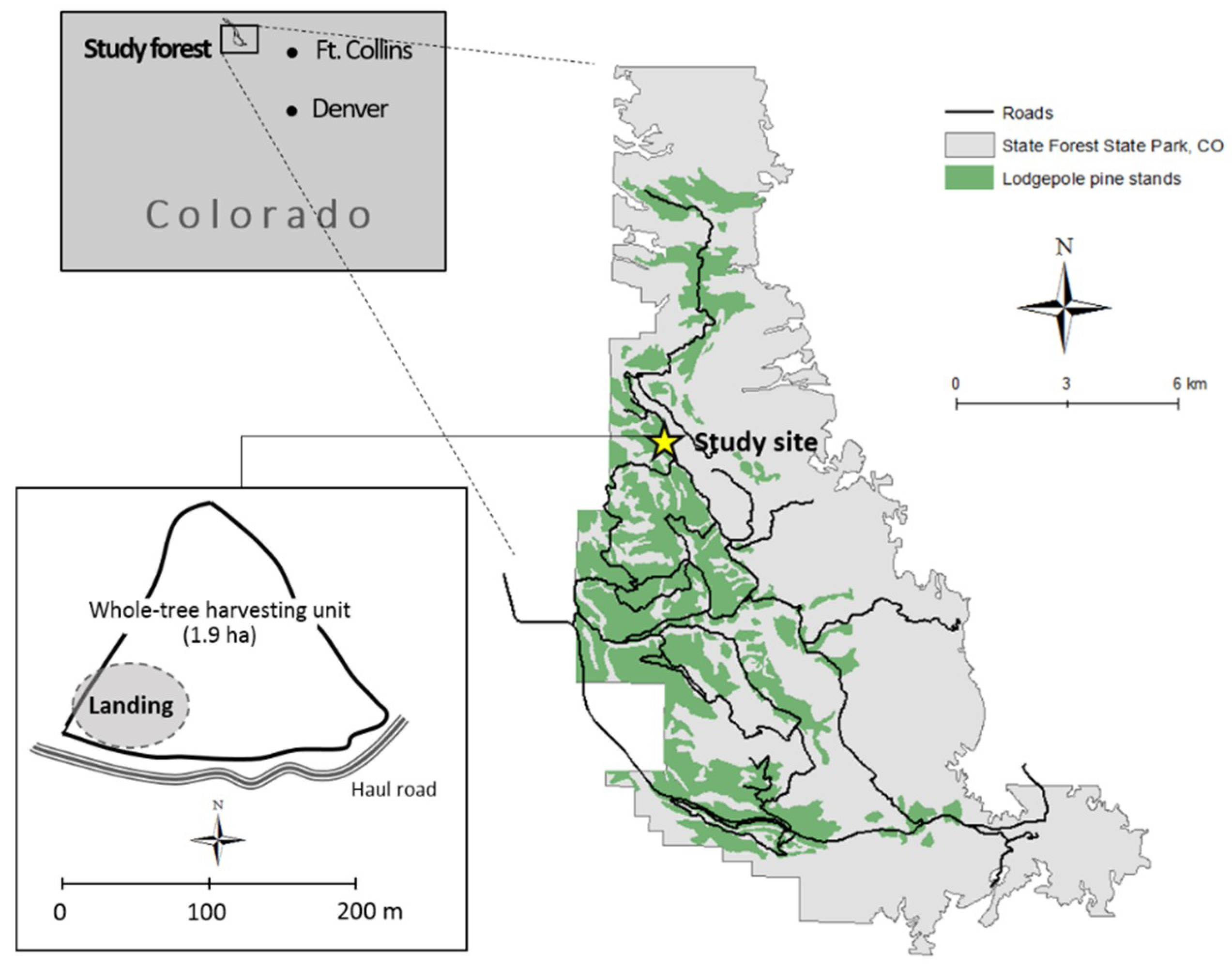
We conducted a time study on a ground-based, whole-tree clear cut of the beetle-killed lodgepole pine (Pinus contorta Dougl. ex. Loud. var. latifolia) harvest unit located in Colorado State Forest State Park (Figure 1) in northern Colorado (40°35′59″ N, 106°00′27″ W) [36]. This 1.9-ha unit was affected by the mountain pine beetle outbreak since 2008 and the mortality rate in 2015 was 47.3%. The stand density was 865 trees ha⁻¹ and the average basal area was 34.6 m² ha⁻¹. The mean diameter at breast height (dbh) of trees was 22.4 cm and the mean height was 19.6 m. Due to the small tree size, most trees were processed into only one piece of log. Post harvesting, we sampled 28 logs to measure small end diameter and length. These measured data were used to estimate oven dry log weight [37], resulting in an average of 0.1185 oven dry ton (odt) per piece.

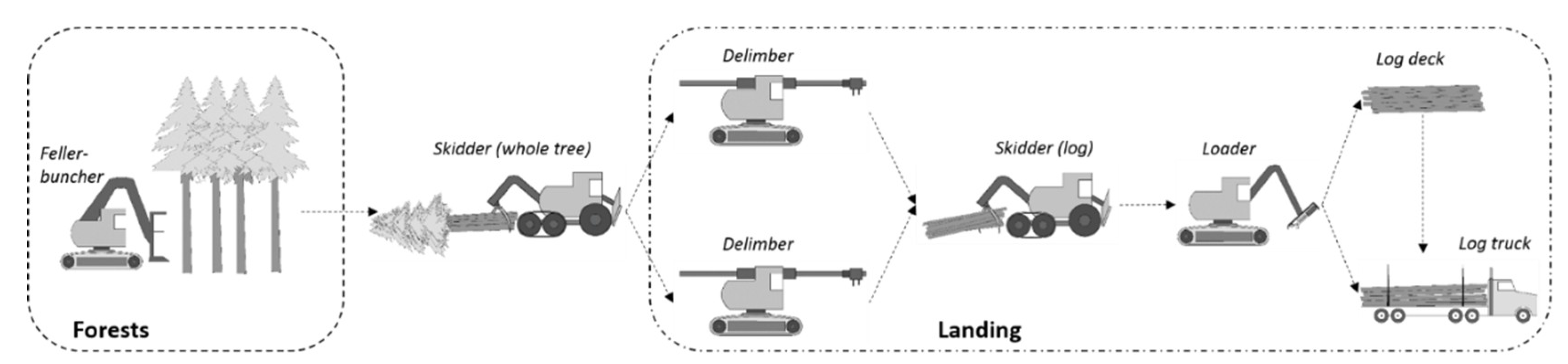
The WT system consisted of one tracked feller-buncher for cutting trees down (TimberPro TL-735-B, TimberPro Inc., Shawano, WI, USA), one grapple skidder (Tigercat 615C, Tigercat Industries Inc., E. Brantford, ON, Canada) for primary transportation (i.e., from stump to landing), two stroke boom delimbers (Timberline SDL2, DDI Equipment, Whitewater, CO, USA) for delimbing and bucking, and one grapple loader (Barko 495ML Magnum, Barko Hydraulics, LLC, Superior, WI, USA) for sorting, decking, and loading logs (Figure 2). All equipment was operated by experienced operators and worked simultaneously on site. Cut trees were transported to the landing by the skidder in the form of whole trees. The delimbers staying close to the landing processed trees into logs. When there was a truck on site, the loader performed sorting and loading simultaneously by directly loading some logs onto the truck while placing other logs (i.e., different sorts) onto the deck. When no trucks were on site, the loader performed only log sorting and decking.

Following standard work study methods [2,17], we collected detailed time study data in December 2015 from the harvesting unit. Readers are referred to Han et al. [36] for a detailed description of the WT harvest unit and field data collection.

Table 1. Field-collected data and applications in models.

Equipment	Data	Value Range	Mean	Application
Feller-buncher	Felling time (s)	7–71	20.8	Both
	Move distance (m)	0–11.6	0.9	TS
	Number of standing trees	0–4	1.9	Both
	Number of down trees	0–2	0.1	Both
	Tree pile size	9–20	14.5	DES
	Relocation chance (0 = no, 1 = yes)	0 or 1	0.05	DES
	Relocation time (s)	11–63	46.0	DES
Skidder (Tree)	Empty travel time (s)	60–128	88.6	Both
	Positioning and grappling time (s)	12–33	20.8	Both
	Bunching time (s)	25–130	40.7	Both
	Loaded travel time (s)	58–145	86.1	Both
	Empty travel distance (m)	82.6–219.8	165.0	Both
	Loaded travel distance (m)	43.9–230.7	141.3	Both
	Number of trees	9–40	21.9	Both
Skidder (Log)	Empty travel time (s)	22–43	35.1	Both
	Positioning and grappling time (s)	5–18	8.9	Both
	Loaded travel time (s)	11–42	21.0	Both
	Empty travel distance (m)	29.0–63.7	44.3	TS
	Loaded travel distance (m)	6.7–43.6	27.1	TS
	Number of logs	9–40	22.9	TS
Delimber	Delimbing time (s)	12–104	42.3	Both
	Reposition chance (0 = no, 1 = yes)	0 or 1	0.1	DES
	Positioning time (s)	9–88	29.8	DES
	Number of live trees	0–5	0.76	Both
	Number of dead trees	0–5	0.92	Both
Loader	Sorting and decking time (s)	6–119	36.4	Both
	Loading time * (s)	11–115	43.7	Both
	Task (0 = sort and deck, 1 = direct loading)	0 or 1	0.30	TS
	Direct loading chance † (0 = no, 1 = yes)	0 or 1	0.50	DES
	Number of logs	1–14	3.3	Both

* Loading cycle time data include both direct loading and loading from deck. ^† Proportion of direct loading while a truck is on site. TS = time study, DES = discrete-event simulation.

shows cycle time elements and corresponding operational data for each machine and their applications in building TS and DES models. Some data were only used in the DES model because they were not related to delay-free machine cycles. Some other data were only used in the TS model because they were identified as independent variables of regression models whereas the DES model used other information to describe the same processes.

Hourly machine costs (

Table 2. Estimated hourly costs of each machine in the study.

Cost Component	Feller-Buncher		Delimber		Skidder		Loader
	Operating	Idle	Operating	Idle	Operating	Idle	Operating	Idle
Sale price ($)	395,000	395,000	355,000	355,000	219,000	219,000	205,000	205,000
Salvage value ($)	59,250	59,250	71,000	71,000	32,850	32,850	61,500	61,500
Machine life (year)	5	5	5	5	5	5	5	5
Depreciation ($/year)	67,150	67,150	56,800	56,800	37,230	37,230	28,700	28,700
Interests ($/year)	26,070	26,070	24,140	24,140	14,454	14,454	14,760	14,760
Insurance ($/year)	10,428	10,428	9656	9656	5781.6	5781.6	5904	5904
SMH (h/year)	2000	2000	2000	2000	2000	2000	2000	2000
Fixed cost ($/h)	51.82	51.82	45.30	45.30	28.73	28.73	24.68	24.68
Fuel (L/h)	29.9	3.0	32.0	3.2	23.3	2.3	14.2	1.4
Fuel ($/h)	17.46	1.75	18.68	1.87	13.61	1.36	8.28	0.83
Lubricant ($/h)	6.46	0.65	6.91	0.69	5.04	0.50	3.06	0.31
R & M * ($/h)	55.96	0	39.32	0	27.92	0	19.87	0
Labor ($/h)	34.29	34.29	34.29	34.29	34.29	34.29	34.29	34.29
Operation cost ($/h)	114.16	36.68	88.29	36.85	80.86	36.16	65.50	35.42
Total cost ($/h)	165.99	88.51	144.51	82.15	109.60	64.89	90.19	60.11

* Repair and maintenance cost proportional to machine depreciation and utilization, adapted from [9]. SMH = scheduled machine hours.

) were estimated using the commonly accepted machine rate calculation method [9,38]. In addition to machine fixed and operation costs, we distinguished machine idle costs from operating costs to differentiate costs related to machines idling (e.g., operational delay, warm-up, etc.). This is deemed necessary because some machine operating costs, such as for fuels and lubricants, are lower during idle time. We assumed the fuel consumption rate during idle times is 10% of the productive time rate [39,40].

2.2. Model Building

Detailed time study data were used to build both DES and TS regression models to evaluate the stump-to-truck harvesting process of the WT system. Two thirds of the cycle time data were randomly selected for model construction and the rest were used for model validation. In the DES model, time element data and other observed operational data were used to create discrete events of each machine process and corresponding input probability distributions. In the TS model, cycle time data were used as dependent variables to build delay-free cycle time equations for each machine based on independent variable values. Both models (referred to as base DES and TS models) were applied to the harvesting of 1700 trees where the average skidding distance was 152 m. The system productivity per scheduled machine hour (SMH) and the timber stump-to-truck cost estimated by both models were compared to show the differences between these two modeling approaches. The DES and TS models are described in detail below.

2.2.1. Discrete-Event Simulation Models

We constructed our DES model in the Rockwell Arena simulation software [41], which has been widely used as a DES simulation tool for both research and practical applications [42,43]. In the simulation, entities are used to represent objects (e.g., products, customers) that are processed by resources (e.g., machine, labor) of the modeled system. They flow through the system from one resource to another, triggered by the occurrence of events. Events themselves occur due to the arrival of entities, the completion of process tasks, random equipment failures, and other related items (e.g., break times). The model generates random realizations of these operational items from the user-defined probability distributions representing their durations. In this manner, events occur and entities move through the system over time until the simulation meets the designated terminating condition (e.g., the completion of processing of all entities, a certain length of simulation time). The DES model is normally run multiple times and provides summary statistics of the simulation results in order to account for uncertainties that may exist in the system [44].

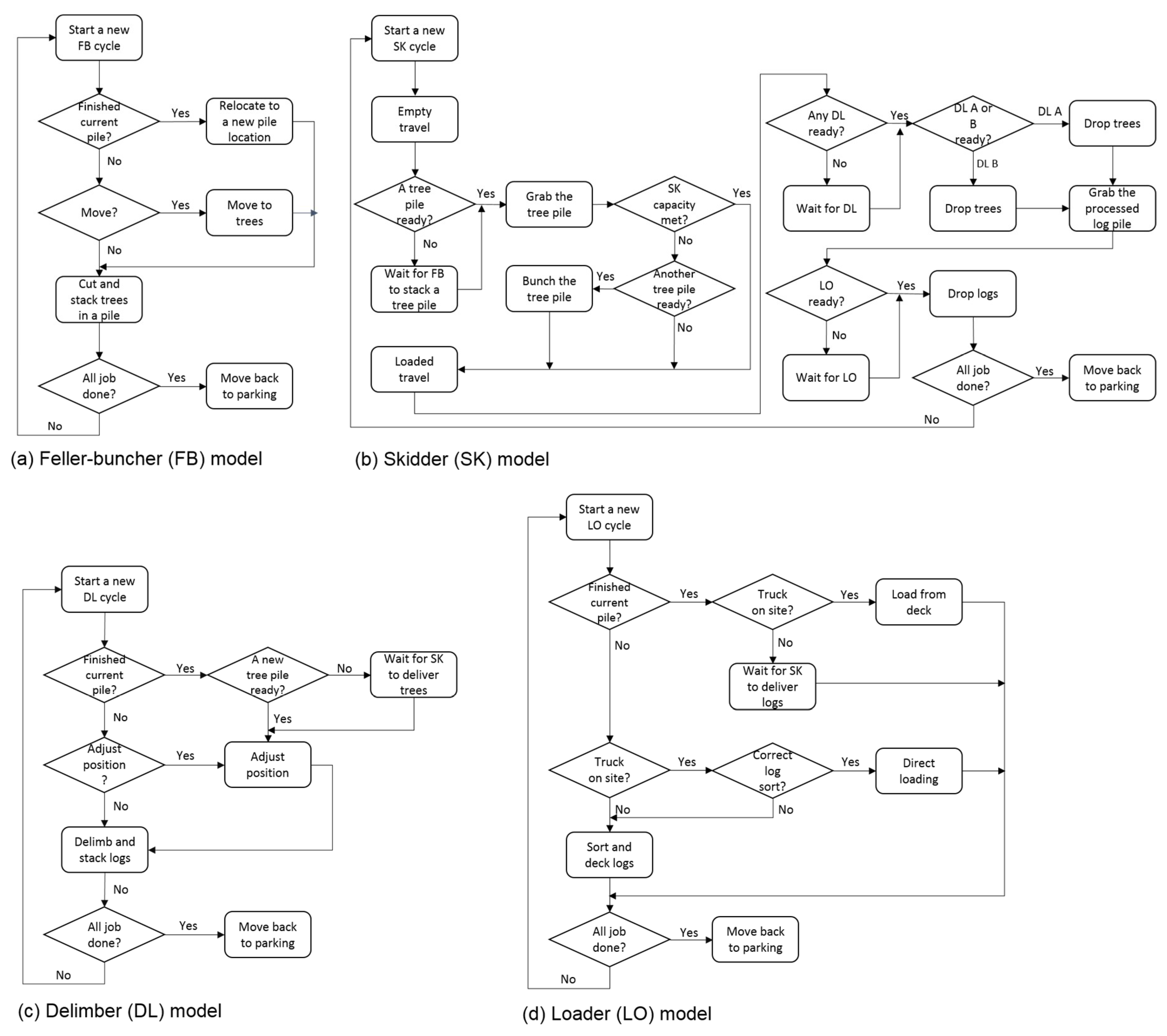
In our study, trees/logs were modeled as entities and machines were modeled as resources. All procedures related to the harvesting process, such as machine processing times, machine reposition probabilities, the number of trees/log pieces in a machine cycle, etc. were modeled within the simulation. To derive appropriate probability distributions for these procedures, several theoretical distributions in the form of mathematical formulations (e.g., Exponential, Gamma) were statistically “fit” to the field time study data. The quality of fit was determined by the Chi-square Goodness-of-Fit test and all proposed distributions were ranked by p-values from high to low. A p-value greater than 0.05 indicated an acceptable fit and the distribution could be used in the simulation model. If no theoretical distributions were acceptable, an empirical distribution was used, which merely divided data into groups with values representing proportions of data in each group. For example, the number of trees that were delimbed in a delimbing cycle followed an empirical distribution, and the time used for delimbing one tree was drawn from an Erlang distribution. The final fitted distributions of all modeled processes are listed in

Table 3. Fitted distributions for each event of machine operations.

Equipment	Event	Distribution	Arena Expression *	p-Value
Feller-buncher	Relocation chance	Empirical	DISC (0.95, 0, 1, 1)	-
	Relocation time	Empirical	CONT (0.00, 10.50, 0.29, 23.50, 0.64, 36.50, 0.86, 49.50, 1, 63.50)	-
	Down tree cycle chance	Empirical	DISC (0.94, 0, 1, 1)	-
	Down tree cycle time	Beta	11.5 + 31 × BETA (1.57, 1.47)	0.30
	Cycle cut piece	Empirical	DISC (0.22, 1, 0.85, 2, 0.96, 3, 1, 4)	-
	One-piece felling time	Erlang	4.5 + ERLA (2.57, 4)	0.37
	Two-piece felling time	Erlang	7.5 + ERLA (2.4, 5)	0.09
	More-piece felling time	Gamma	12.5 + GAMM (3.25, 3.37)	0.17
	Tree pile size	Weibull	8.5 + WEIB (6.73, 2.06)	0.06
Delimber	Reposition chance	Empirical	DISC (0.90, 0, 1, 1)	-
	Reposition time	Erlang	8.5 + ERLA (10.7, 2)	0.36
	Cycle cut piece	Empirical	DISC (0.53, 1, 0.87, 2, 0.94, 3, 1, 4)	-
	One-piece delimb time	Erlang	11.5 + ERLA (4.96, 5)	0.23
	Two-piece delimb time	Gamma	12.5 + GAMM (7.67, 4.13)	0.17
	More-piece delimb time	Beta	27.5 + 54 × BETA (1.36, 1.59)	0.12
Skidder	Empty distance ratio †	Triangular	TRIA (0.55, 1.15, 1.57)	0.14
	Loaded distance ratio	Triangular	TRIA (0.09, 0.77, 1)	0.49
	Empty speed	Triangular	TRIA (1.41, 1.91, 2.27)	0.27
	Loaded speed	Triangular	TRIA (0, 1.27, 2.44)	0.06
	Skid log trip	Triangular	TRIA (49.5, 67, 88.5)	0.44
Loader	Loading piece	Poisson	POIS (2.88)	0.74
	Direct loading chance	Empirical	DISC (0.51, 0, 1, 1)	-
	Loading time	Beta	13.5 + 69 × BETA (1.27, 1.91)	0.36
	Sort and deck piece	Poisson	POIS (3.45)	0.31
	Sort and deck time	Erlang	5.5 + ERLA (7.35, 4)	0.24

* In Arena expression, DISC (CumP1, Val1, …, CumPn, Valn) and CONT (CumP1, Val1, …, CumPn, Valn) are empirical distributions showing pairs of cumulative probabilities and associated values. For other distributions (i.e., BETA, ERLA, GAMM, WEIB, TRIA and POIS), input values are parameters specified according to distribution mathematical forms. More details on Arena’s probability distribution can be found in [44]. ^† The skidder empty travel distance in each trip was estimated to be proportional to the average skidding distance. In the same trip, the skidder loaded travel distance was estimated to be proportional to the empty travel distance.

. Events were connected by logical links developed to form the structure and logic of the DES model (Figure 3). A simulation run began as the feller-buncher started cutting trees. Trees/logs were then processed by each machine following the order in practice. For a feller-buncher cutting cycle, the model first determined if a machine relocation was necessary prior to cutting based on the machine relocation probability. If yes, the model randomly drew a relocation time from the relocation time distribution and added it to the machine cycle time. The model then generated the number of trees cut for the cycle and assigned a cutting time randomly drawn from the cutting time distribution. After completing one tree-cutting cycle, the feller-buncher was ready for the next cycle and trees were stacked in a pile waiting to be transported by the skidder.

The skidder started a new cycle with an empty travel from the landing to a tree pile. Travel time was estimated using travel distance and speed that were randomly drawn from the user-defined distance and speed distributions. When the skidder arrived at a tree pile, the skidder operator checked if the pile was ready for transportation; if not, the operator had to wait for the feller-buncher to finish cutting trees and completing a tree pile. The skidder grabbed a tree pile otherwise, and then sought another tree pile to combine if the capacity was not met yet. As the skidder travelled loaded towards the landing, the operator checked if any of the two delimbers had completed processing of the previously delivered trees. If no delimber was available, the skidder waited until one delimber was ready, and then passed the trees onto the available delimber. The skidder then grabbed the processed logs and skidded them to the loader. Similarly, the operator checked the loader’s availability before passing logs.

The delimber operator started a new cycle by checking if the previous tree pile had been finished. If there was no tree to delimb, the operator stayed idle and waited for the skidder to deliver trees. If there were trees from the previous pile, the model determined if the delimber needed to adjust machine position before delimbing. If yes, it added a reposition time. The model then randomly generated the number of trees and delimbing time to complete the delimbing cycle. Processed logs were stacked in a log pile and readied for pick up by the skidder that delivered a log pile to the log deck at the landing.

The loader had different tasks depending on the availability of log trucks and sorted logs. When the skidder delivered logs and a truck was available on site, the loader operator simultaneously sorted logs and loaded the requested sort onto the truck (“direct loading”). When a truck was available but there were no more logs to sort, the loader loaded the previously sorted and decked logs onto the truck (“load from deck”). When no truck was available at the landing, the loader operator sorted logs and stacked them on the deck (“sort and deck”). When neither logs to sort nor trucks were available, the loader stays idle.

Because long-term shift level information was not available, assumptions were made during the simulation in order to setup work shifts and machine breakdowns. A work day was assumed to be 10 SMH with a 45-min machine warm-up period in the morning and 45-min machine maintenance work at the end of day. Five trucks were scheduled to visit the harvest site to haul logs and their inter-arrival time was assumed to be normally distributed (i.e., NORM (60, 15) in Arena). For all equipment, machine failures might occur at any time. The failure rate and repair times were assumed to follow an exponential distribution with parameters of 1000 and 30 min (i.e., EXPO (1000) and EXPO (30) in Arena), respectively. For each machine, time spent on operation, warm-up and maintenance, idle state, and other disturbances (e.g., repair, personal delay) were categorized as utilization, scheduled delay, operational delay, and other delays. Scheduled delays included machine warm-up and scheduled maintenances, while operational delays were mainly caused by machine interactions (i.e., time spent to wait until other machines finish their cycles). When all harvested logs were delivered to the landing, all the machines except for the loader stopped working and returned to their parking spots. The loader continued working until all harvested logs were loaded onto trucks. Once all logs were loaded, a single simulation run was considered completed. In this study, a total of 100 simulation runs were made.

2.2.2. Time Study Regression Models

We adopted the multiple least-squares linear regression models in [36] for most machines in our TS models except for the skidder. In this study, we developed two separate regression equations (R Statistical Software version 3.4.0 [45]) for the skidder to estimate delay-free cycle times of two different tasks: skidding trees to the delimbers at the landing, and skidding logs from the delimbers to the loader. A tree skidding cycle included empty travel from the landing, grabbing trees, bunching trees, loaded travel and dropping trees. A log skidding cycle included empty travel to a processed log pile, grabbing logs, loaded travel to the loader, and dropping logs.

For each machine, the average values of independent variables were used to predict the mean delay-free cycle times. Combined with the average processed log volume in each machine cycle, hourly productivities in PMH were calculated for all equipment. Because TS models were static, machine interactions and different types of delays could not be captured by the model. Instead, machine productivities in PMH were converted to productivities in SMH by applying the following empirical utilization rates [9,36]: 60% for the feller-buncher, 65% for the delimbers, 60% for the skidder, and 65% for the loader. A machine with the lowest SMH productivity became the system bottleneck and its productivity was used for the entire system productivity. As the result, unit production costs, resulting machine utilization rates, and unutilized machine times (categorized as delay) were estimated.

2.3. Sensitivity Analysis

The average skidding distance normally has a large influence on the skidder’s cycle time, productivity, interactions with other machines, and ultimately the performance of the entire system. We conducted a sensitivity analysis to evaluate the impact of the average skidding distance on both the DES and TS models. Different average distances were used ranging between 50 and 600 m with an increment of 50 m. The results from the DES and TS models are compared in terms of system productivity, unit production cost, and machine utilization rates.

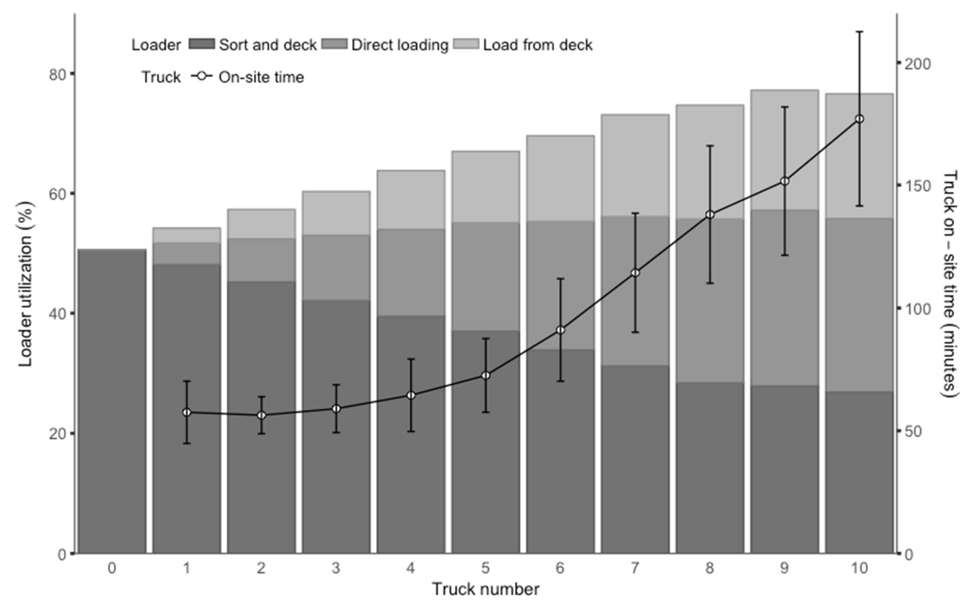
We also examined the sensitivity of the DES model to truck availability to assess how the harvest system responds to different number and frequency of trucks. In our studied system, the loader serves as a link between in-woods harvesting operations and truck transportation. Different trucking schedules likely affect the loader’s work pattern and its interactions with other machines. Truck scheduling has been traditionally dealt with as a separate problem from stump-to-landing operations in forest operations analysis, but it may become an important factor for operational efficiency when harvesting units have limited space for landing and log decking. Using the DES model, we varied the number of trucks on site from 0 to 10 trucks per day and examined its influence on the loader’s utilization, time used for different tasks, and truck on-site time. We were not able to estimate the impact of different truck schedules using the TS approach because TS regression models were static and the loader’s interactions with trucks were impossible to model with our limited data. Therefore, we did not make comparisons between the DES and TS models for varying truck schedules.

2.4. Hypothetical Systems

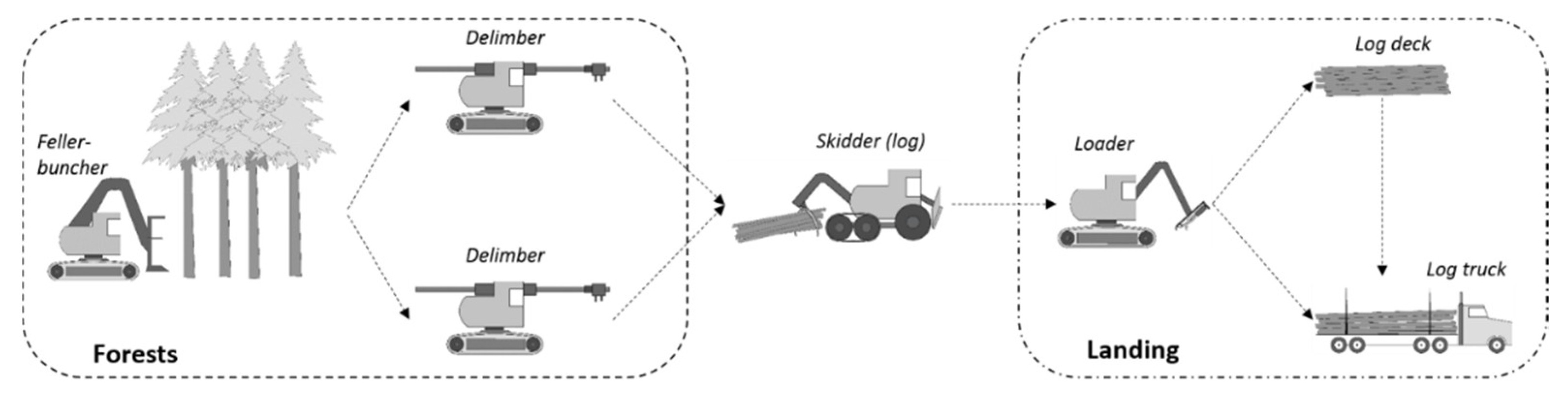
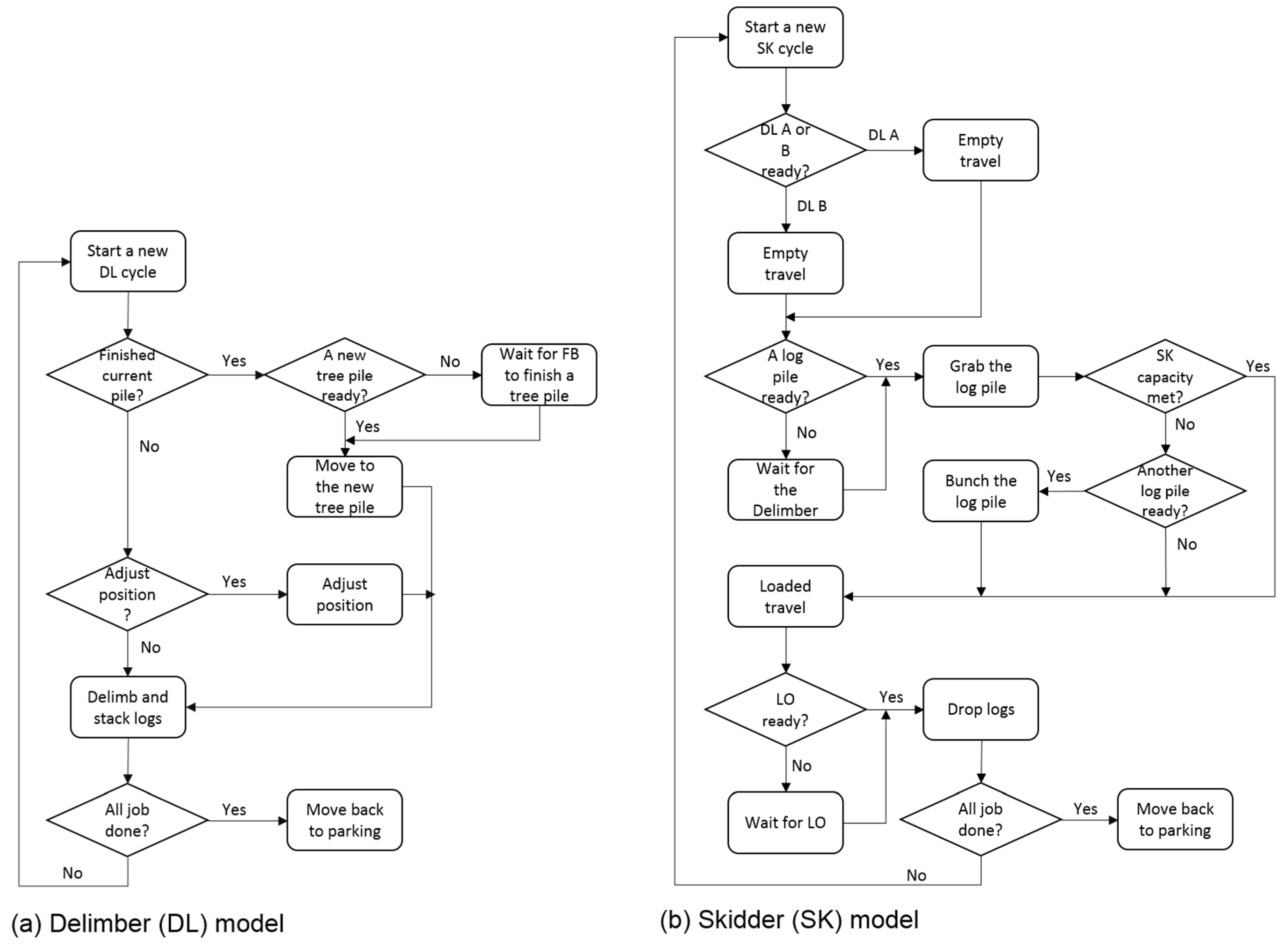
To demonstrate the potential advantage of DES models in analyzing hypothetical systems, we built a new DES model to simulate another ground-based harvesting system called lop-and-scatter (LS) [36]. The LS system employs the same machines as the WT system, but with differences in the delimbing location and the order of operations (Figure 4). In LS, the delimber processes trees at the stump instead of at the landing, leaving limbs and tree tops in the woods. The skidder then forwards the processed logs to the loader at the landing.

For the DES model developed for the LS system (hereafter referred to as LS DES), we used the same discrete events and input probability distributions as those used in the previous DES model developed for the WT system (hereafter referred to as WT DES). A new additional event required for the LS DES model was a delimber’s in-woods movement from tree pile to pile. For this, we used a delimber’s reposition time distribution as a substitution. Logical links were developed to connect sequential events necessary for the LS system (Figure 5). In this system, the delimbers directly interact with the feller-buncher, while the skidder transports only processed logs from stump to landing.

The LS DES model was run under the same harvesting conditions used in the WT DES model. The results were then compared with our independent data obtained from the LS operations conducted in the same unit in Colorado State Forest State Park for model validation [36].

The field LS data were also used to develop a new TS model for the LS system (LS TS). We compared the results of the LS TS model with the LS DES model. For further analysis, we used two sets of machine utilization rates when converting machine productivities in PMH to those in SMH. The first set is the general utilization rates [9] used in the WT TS model. The other set is the utilization rates resulting from the LS DES model. Estimations from these two approaches are referred to as LS TS_conventional and LS TS_adjusted, and are compared with the outputs from the LS DES model in terms of system productivity in SMH and unit production cost to further highlight the importance of machine utilization rates in system performance evaluation.

3. Results

3.1. DES and TS Models for Whole-Tree Harvesting

The results of 100 simulation runs of the base WT DES model are presented in

Table 4. Performance metrics of individual machines and the entire system of whole-tree harvesting generated by 100 simulation runs of the DES model. Standard deviations are shown inside parentheses.

Machine	Cycle Time * (s)	Productivity (odt/PMH)	Utilization (%)	Sys. Prod. (odt/SMH)	Unit Cost ($/odt)
Feller-buncher	20.5 (1.5)	41.83 (0.66)	51.7 (4.2)	20.16 (1.71)	29.71 (1.92)
Delimber A	42.5 (3.0)	17.14 (0.35)	61.6 (6.1)
Delimber B	42.9 (3.0)	17.08 (0.40)	56.3 (6.0)
Skidder (trees)	256.0 (3.1)	39.86 (1.71)	64.5 (5.2)
Skidder (logs)	71.3 (9.1)	145.01 (4.49)
Loader (loading †)	42.2 (3.0)	29.43 (1.86)	66.9 (4.5)
Loader (sort and deck)	36.4 (3.0)	40.17 (1.31)

* Delay free cycle time. ^† Loading includes both direct loading and load from deck. odt = oven dry ton, PMH = productive machine hours.

. Individual machine process productivities ranged from 17.08 to 145.01 odt/PMH with log processing by delimber B having the lowest productivity and log skidding by the skidder having the highest productivity in the system. The utilization rates were fairly even among the individual machines except for the feller-buncher that had the lowest rate of 51.7%. The entire system productivity was 20.16 odt/SMH and unit production cost was estimated at $29.71/odt. The coefficient of variation (i.e., the ratio of standard deviation to the mean) was less than 7% for all the machines, indicating the simulated machine processes were not variable among simulation runs.

Table 5. Delay-free cycle time regression models for individual machines used in whole-tree harvesting (adopted from [36]).

Machine	Average Cycle Time Estimator (s)	SE	t	p-Value	$\mathbf{Adj}.{\mathit{R}}^2$	Model p-Value
Feller-buncher	=10.140	0.614	16.50	<0.01	0.4329	<0.01
	+ 3.709 × No. of standing trees	0.296	12.54	<0.01
	+ 13.082 × No. of down trees	0.870	15.04	<0.01
	+ 0.301 × move dist. (m)	0.025	12.29	<0.01
Delimber	=30.765	1.522	22.22	<0.01	0.1898	<0.01
	+ 6.624 × No. of live trees	0.913	7.25	<0.01
	+ 5.729 × No. of dead trees	0.961	5.96	<0.01
Skidder (trees)	=25.125	47.53	0.529	0.603	0.5976	<0.01
	+ 0.192 × empty travel dist. (m)	0.099	1.944	0.066
	+ 0.145 × loaded travel dist. (m)	0.073	1.983	0.061
	+ 1.881 × No. of trees	0.984	1.913	0.070
Skidder (logs)	=42.290	6.964	6.073	<0.01	0.2625	<0.01
	+ 0.890 × No. of logs	0.312	2.850	0.010
Loader	=22.006	1.892	11.629	<0.01	0.2033	<0.01
	+ 3.739 × No. of logs	0.471	7.937	<0.01
	+ 8.248 × loading activity (1 or 0)	1.794	4.597	<0.01

presents the delay-free cycle time regression models used in this study for the TS approach. Each regression model was tested for assumptions of normality, independence and equal variance in order to ensure the validity of regression analysis. No serious violations were identified, and all models were significant (p < 0.05). The TS model predicted the system productivity and unit production cost to be 18.67 odt/SMH and $30.21/odt, respectively (

Table 6. Performance metrics of individual machines and the entire system of whole-tree harvesting predicted by the TS model.

Machine	Cycle time * (s)	Productivity (odt/PMH)	Utilization (%)	Sys. Prod. (odt/SMH)	Unit cost ($/odt)
Feller-buncher	19.5	41.83	44.6	18.67	30.21
Delimber A	41.1	17.53	53.3
Delimber B	41.1	17.53	53.3
Skidder (trees)	237.5	39.33	60
Skidder (logs †)	62.6	148.29
Loader (loading §)	42.5	28.89	48.8
Loader (sort and deck)	34.3	42.94

* Delay free cycle time. ^† Calculated by assuming equal number of skidding tree process and skidding log process. ^§ Calculated with the assumption that loader spends 30% and 70% of its times on direct loading, and sorting and decking, respectively.

). The skidder became the system bottleneck due to its lowest productivity in SMH after conversion using the generalized utilization rate. The feller-buncher was predicted to have the highest productivity and therefore the lowest utilization in the system.

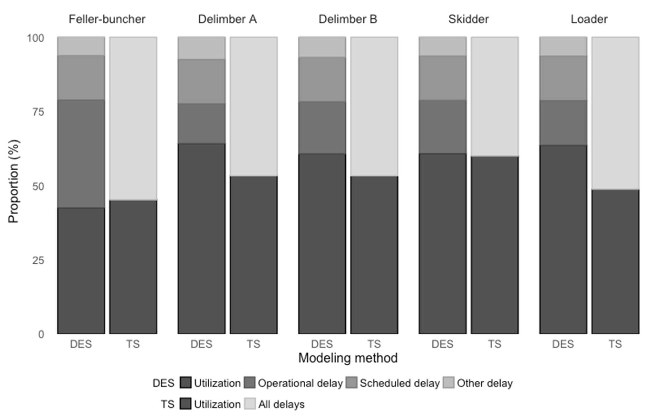
The comparisons of machine productivity between the estimated values and the field-observed values in the validation data set show that the estimated average machine productivities of all equipment by both models deviate less than 9% from the observed values (

Table 7. Comparison of the estimated mean machine productivities obtained from the WT DES and TS models with the field-observed productivities for whole-tree harvesting.

Machine	Observed Productivity (odt/PMH)	Difference * (%)
		DES	WT
Feller-buncher	42.75	−2.1	−2.2
Delimber A	17.30	−1.0	1.3
Delimber B	17.30	−1.3	1.3
Skidder (tree)	37.30	6.9	5.4
Skidder (log)	153.18	−5.3	−3.2
Loader (load)	27.78	5.9	4.0
Loader (sort and deck)	39.54	1.6	8.6

* Percentage difference between model estimates and the observed values. WT = whole-tree harvesting, DES = discrete event simulation, TS = time study.

). The DES model has better estimates of productivity for the feller-buncher, skidder and loader, while the TS model has better estimates for the delimbers. The biggest difference was found with the loader “sort and deck” process where the TS model overestimated the productivity by 8.6%. As for machine utilization, the two models reported similar rates for all machines but the loader (Figure 6). For the feller-buncher, delimbers and skidder, the minor differences in machine utilization rates by the two models mainly came from the differences in estimated machine productivities and the system productivity. In the DES model, Delimber A had a higher utilization than Delimber B because during the simulation it was assigned as the primary resource, which means Delimber A is used first if delimbers were available. In the TS model, the two delimbers were equally treated. For the loader, the difference in the reported utilization is apparent. The TS model reported lower utilization because it only included “direct loading” and “sort and deck” whereas the DES model also considered “load from deck” processes. The occurrence of this last process depends on the status of the loader (i.e., no log pile to sort and load) and the truck (i.e., available on site). The TS model could not assess this situation so that it overestimated loader productivity and underestimated the loader utilization.

The DES model was also able to provide both delay type and quantity of each machine. The amount of scheduled delays and other delays were similar across all machines, while the feller-buncher had the largest proportion of operational delay because of its high productivity and interactions with lower productivity machines. Due to the variation of operations and interdependencies among machines, there was no “absolute” system bottleneck and all other machines experienced a certain amount of operational delays. The TS model was able to estimate only the overall utilization of individual machines based on their published empirical utilization rates (or long-term utilization rates) and the bottleneck machine’s productivity. The feller-buncher had the largest overall delays as well in the TS model due to its high productivity compared to the other machines. The skidder was the system bottleneck and its utilization rate was estimated to be equal to the empirical rate.

3.2. Sensitivity Analysis

3.2.1. Skidding Distances

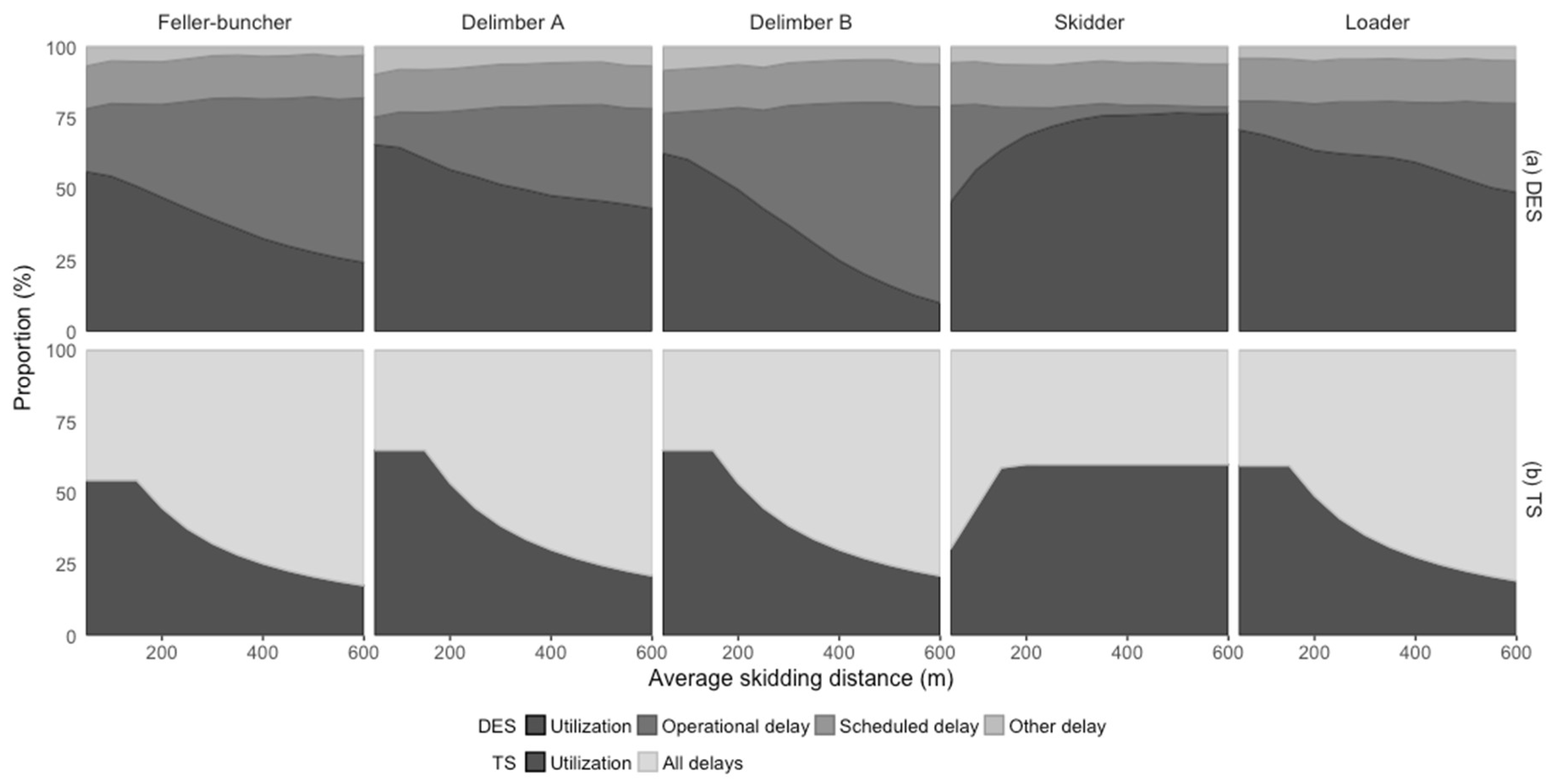
The utilization rates of individual machines changed with different skidding distances (Figure 7). The results show that operational delays of individual machines varied widely across different skidding distances, while the proportions of scheduled and other delays were relatively constant over the range of skidding distance. A longer skidding distance increased the skidder’s cycle time and utilization, and decreased its operational delay, while it increased operational delays of all the other machines. This indicates the skidder becomes the system bottleneck causing the delimbers and the loader to wait for the skidder to supply logs. As skidding distance increases, the feller-buncher appears to experience increased operational delay because it has to spend a longer time waiting for the other machines. The TS model shows similar patterns of changes in total delays but with more abrupt transitions as skidding distance increases. This is because the utilization rate of the bottleneck machine is assumed to be constant.

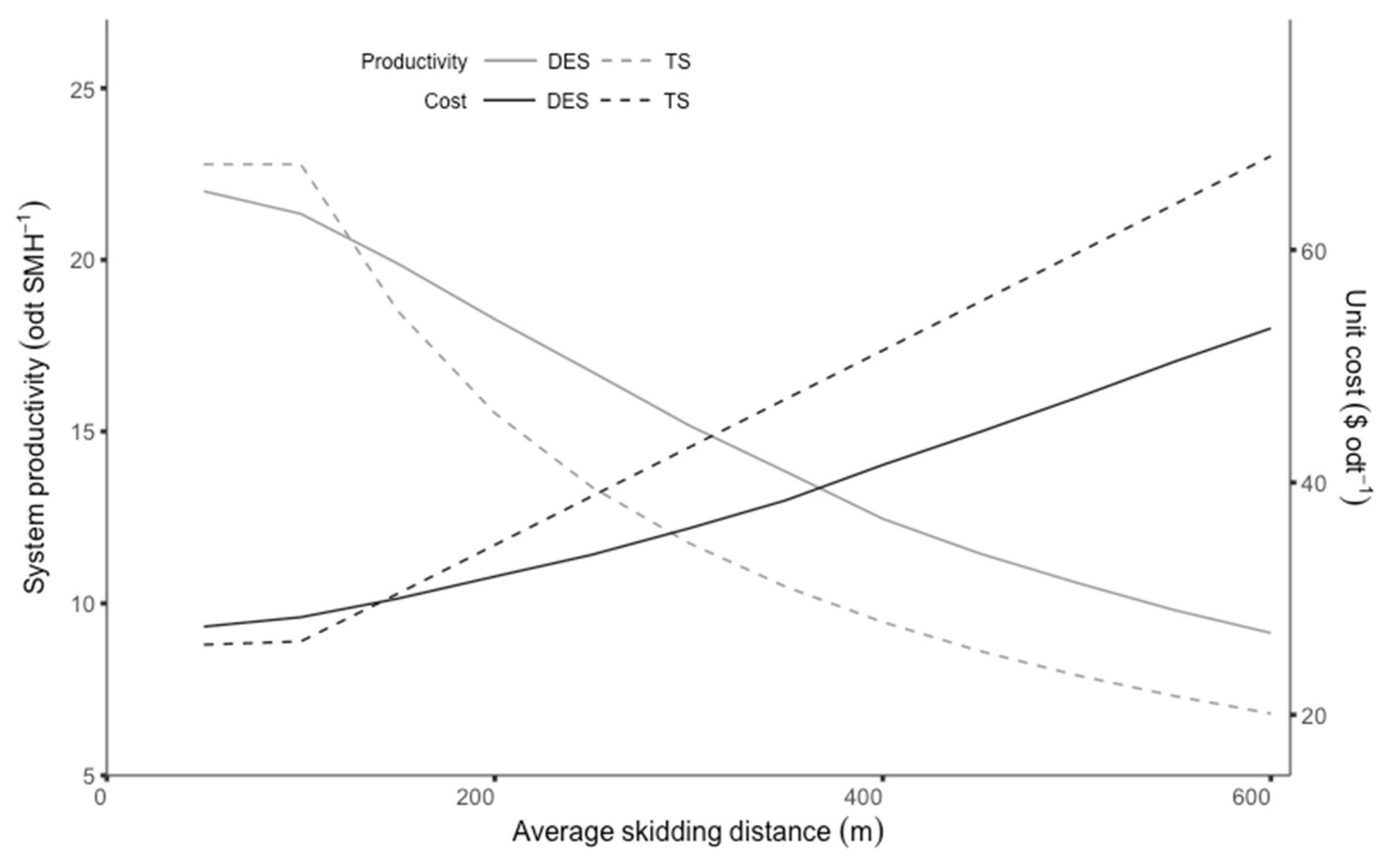
The productivity of the entire system and its unit production cost also change in response to different skidding distances (Figure 8). Overall, the estimated system productivity decreased and the unit cost increased as skidding distance increased in both models. However, when skidding distances were relatively short (i.e., less than 100 m), the TS model estimated the system productivity and unit cost to be constant, whereas the DES model showed gradual changes. This is because for the short skidding distances the delimber was the system bottleneck and skidding distance does not influence the system cost nor the productivity in the TS model. The DES model, however, was able to capture changes in skidder efficiency caused by different skidding distances and incorporate them into system productivity and cost estimation.

3.2.2. Trucking Schedules

The DES model estimated the utilization rate of the loader at about 55% when no trucks were scheduled (Figure 9). The utilization rate increased by approximately 2% per truck as more trucks were scheduled to pick up the logs. The results show that the loader spends an increasing amount of time in “direct loading” as more trucks are scheduled. On the other hand, the truck on-site time, which includes truck waiting time in queue and truck loading time, increased due to higher chances of queueing. When the scheduled truck number was less than four, the truck on-site time had an average of 60 min and a standard deviation of 15 min. Beyond that, the on-site time increased quickly in both the average and standard deviation. With 10 trucks visiting the harvesting site per day, the loader would spend about 30%, 25% and 25% of its productive times on “direct loading”, “load from deck”, and “sort and deck”, respectively, with a total utilization rate of approximately 80%. But the truck on-site time had an average of 177 min and a standard deviation of 35 min.

3.3. DES Model for the Lop-and-Scatter System

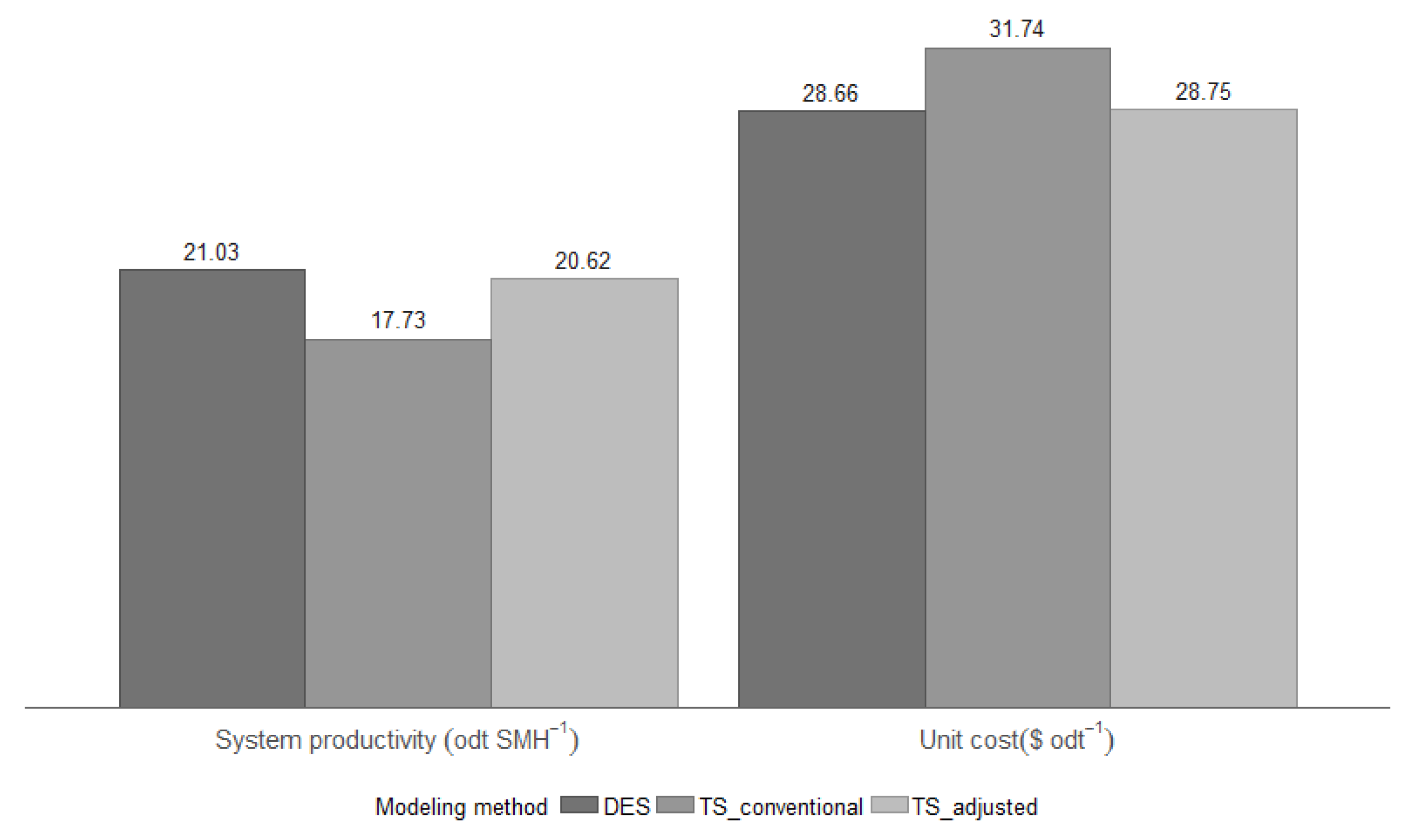
The results of the DES model built for the lop-and-scatter harvesting system using the whole-tree harvesting data show that the estimated machine productivities for individual machines were similar to the field-observed productivities (

Table 8. Comparison of the estimated mean machine productivities obtained from the LS DES model with the field-observed productivities for lop-and-scatter.

Machine	Productivity (odt/PMH)		Difference * (%)
	Observed	DES
Feller-buncher	41.35	41.88 (0.60)	1.3%
Delimber A	13.20	13.81 (0.35)	4.6%
Delimber B	13.20	13.72 (0.40)	4.0%
Skidder	41.07	37.10 (2.02)	−9.7%
Loader (load)	28.40	29.16 (3.98)	−3.4%
Loader (sort and deck)	40.98	39.60 (1.76)	2.7%

* Percentage difference between model estimates and the observed values.

). The biggest difference was with the skidder. The model underestimated the skidder productivity by 9.7% with the observed value being about two standard deviations from the mean estimate. This difference might be attributed to the intrinsic differences between transportation of trees and logs (e.g., turn size). Our comparisons of the LS DES model with the two LS TS models (i.e., TS conventional and TS adjusted) show that the LS DES model estimates were similar to those of TS adjusted, but somewhat different from TS conventional in terms of system productivity and unit production cost (Figure 10). This indicates that both the DES and TS models assess the performance of individual machines similarly when the same, scenario-based machine utilization rates are used as inputs. The results of the TS conventional model were different (15.7% and 10.7% difference in productivity and cost estimates, respectively) because of the published machine utilization rates used in the analysis.

4. Discussion

4.1. Process Synthesis and Model Resolution

Comparing the WT TS and DES model results, the TS model estimated the system productivity to be 7.4% lower and the unit cost to be 1.7% higher (Table 4 and Table 6). The differences were mainly caused by the synthesis procedure for machine processes of the two modeling approaches. The TS model does not track the material flow in the system and thus determines the system productivity as the lowest machine SMH productivity, whereas the DES model is able to keep track of material flow and machine activities as a series of events. As Asikainen [20] noted, static, deterministic models, such as the TS model, generate satisfactory results when the studied system is simple and unbalanced (i.e., apparent bottleneck) but may lead to biased estimates for complex systems.

The ability of capturing operational details in DES modelling is of great value for system improvement. In this study, the TS model was not able to provide information on machine utilization in enough detail to understand the system dynamics (Figure 6 and Figure 7). The DES model, however, could capture machine interactions more precisely by mimicking the actual work pattern and machine-to-machine wood flows. The DES model was able to not only quantify the amount of operational delays but also identify the cause of delays (e.g., the skidder’s operational delays were caused by other “bottleneck” machines, such as the delimber or the loader). While scheduled and other delays are unavoidable in machine operations, the amount of operational delays depicts the efficiency of the harvesting system, and understanding the cause-and-effect of delays can greatly help improve system balance and thus overall efficiency [18].

4.2. Sensitivity Analysis

When TS regression models are applied to a wide range of independent variable values, model extrapolation always becomes a concern. In the TS approach, coefficients in a regression model only infer associations between the dependent and independent variables in the given data set, not necessarily cause-and-effect relationships in general. For example, estimating skidding cycle times based on a linear relationship may produce unreasonable results when the coefficient is applied beyond the original observation range (Figure 7 and Figure 8). The DES approach has a similar restriction because input probability distributions are produced from site-specific data. However, in DES models, a full machine cycle is broken into multiple processes that can be estimated independently. Grappling time, dropping time, skidder empty and loaded traveling speed are still likely to be the same across a wide range of skidding distances, whereas skidder travel times is a direct function of skidding distance. This separate estimation of process times makes the DES models more applicable to a wider range of independent variable values than the TS models. The more gradual changes shown in the DES model outputs from the current study confirmed this benefit (Figure 7 and Figure 8).

The results of our sensitivity analysis on truck availability shows that loader operations and log transportation mutually affect each other. With very few trucks scheduled, the loader has to spend time for “sort and deck” and later “load from deck”, handling logs twice. Increasing the number of scheduled trucks increases the loader “direct loading” time and loader utilization, but too many trucks on site increases the average and variability of truck queue time. This leads to decreased trucking efficiency and increased transportation cost. In a forest supply chain, efficient wood flow from the harvesting system to transportation is critical in reducing logistics costs [46]. The strength of the DES in capturing changes in machine interactions is particularly beneficial to scenario analysis on trucking schedules [29,31]. Our DES model shows the potential tradeoff between loader utilization and truck on-site time (Figure 9) and can be used in operational planning to balance harvesting and transportation efficiency for optimal outcomes.

4.3. Analysis of Hypothetical Systems

In harvesting operations, delay times may vary significantly by system design, as well as stand and terrain conditions [18]. Our study shows that the use of general machine utilization rates in evaluating new harvesting systems (e.g., TS_conventional) may not be appropriate because such utilization rates do not reflect system-specific work conditions, such as machine interactions, that may be caused by a new composition or arrangement of machine processes (Figure 10). A discrete-event simulation of wood flow through a series of machine processes seems more appropriate for new system evaluation because of its ability to address potential machine interactions and precisely estimate the utilization of individual machines. Our finding is consistent with a previous study [30] that compared a DES model with a deterministic spreadsheet model developed for stump crushing and truck transportation.

4.4. DES Model Drawbacks

While the DES approach has many advantages, there are also drawbacks. Special skills are required to build DES models, and the modeling process can be expensive and time-consuming [23]. DES model construction also requires a considerable amount of data, such as time elements of individual machines and their probability distributions, and it is often the case that sufficient data are not available in forest operations to make DES modeling feasible. Although modern data acquisition technologies (e.g., auto-video recording, GPS tracking, sensors) can help access operational data more easily and frequently [47,48,49], long-term field data collection is still necessary to obtain a representative sample of field operations and thus ensure quality output. Also, the large amount of random inputs in DES modeling can make it difficult to interpret the output in simple terms, especially for highly complex systems [50].

5. Conclusions

Our comparison of the TS and DES approaches in modeling a ground-based timber harvesting system indicates that the DES approach may be a more appropriate method for analyzing complex systems especially where interactions among different machine processes are unknown. Randomness and uncertainties can be considered in DES throughout the modeling process to account for variations of operations. Replications of DES model runs enable the user to show a comprehensive picture of the system performance in terms of both average and variability. In addition, the ability of DES to reuse the previously collected data provides an opportunity to evaluate alternative or hypothetical systems that have not been tested in field. Although model construction and output interpretation can be complex and expensive, we believe the potential benefits of the DES approach to provide more comprehensive and precise information that can help identify problematic areas and improvement opportunities in forest operations planning, surpass its potential drawbacks.

References

- Uusitalo, J.; Pearson, M. Introduction to Forest Operations and Technology; JVP Forest Systems Oy: Hämeenlinna, Finland, 2010; ISBN 952-92-5269-2. [Google Scholar]
- Acuna, M.; Bigot, M.; Guerra, S.; Hartsough, B.; Kanzian, C.; Kärhä, K.; Lindroos, O.; Magagnotti, N.; Roux, S.; Spinelli, R.; et al. Good Practice Guidelines for Biomass Production Studies; CNR IVALSA: Sesto Fiorentino, Italy, 2012; ISBN 978-88-901660-4-4. [Google Scholar]
- Schillings, P.L. A Technique for Comparing the Costs of Skidding Methods; Intermountain Forest & Range Experiment Station, Forest Service, U.S. Dept. of Agriculture: Ogden, UT, USA, 1969.
- LeDoux, C.B.; Fight, R.D.; Ortman, T.L. Stump-to-truck cable logging cost equations for young-growth douglas-fir. West. J. Appl. For. 1986, 1, 19–21. [Google Scholar]
- Kellogg, L.D.; Bettinger, P. Thinning Productivity and Cost for a Mechanized Cut-to-Length System in the Northwest Pacific Coast Region of the USA. Int. J. For. Eng. 1994, 5, 43–54. [Google Scholar] [CrossRef]
- Gingras, J.F.; Godin, A. Comparison of Feller-Bunchers and Harvesters for Harvesting Blowdown Timber; Forest Engineering Research Institute of Canada: Pointe-Claire, QC, Canada, 1996; Volume 244. [Google Scholar]
- Han, H.-S.; Lee, H.W.; Johnson, L.R. Economic feasibility of an integrated harvesting system for small-diameter trees in southwest Idaho. For. Prod. J. 2004, 54, 21–27. [Google Scholar]
- Anderson, N.; Chung, W.; Loeffler, D.; Jones, J.G. A productivity and cost comparison of two systems for producing biomass fuel from roadside forest treatment residues. For. Prod. J. 2012, 62, 222–233. [Google Scholar] [CrossRef]
- Brinker, R.W.; Kinard, J.; Rummer, R.; Lanford, B. Machine rates for selected forest harvesting machines. In Machine Rates for Selected Forest Harvesting Maines; Alabama Agric. Expt. Sta., Auburn Univ: Auburn, AL, USA, 2002; p. 32. [Google Scholar]
- Bisson, J.A.; Han, S.-K.; Han, H.-S. Evaluating the System Logistics of a Centralized Biomass Recovery Operation in Northern California. For. Prod. J. 2015, 66, 88–96. [Google Scholar] [CrossRef]
- Kizha, A.R.; Han, H.-S. Processing and sorting forest residues: Cost, productivity and managerial impacts. Biomass Bioenergy 2016, 93, 97–106. [Google Scholar] [CrossRef]
- Mitchell, D.; Gallagher, T. Chipping whole trees for fuel chips: A production study. South. J. Appl. For. 2007, 31, 176–180. [Google Scholar]
- Pan, F.; Han, H.-S.; Johnson, L.R.; Elliot, W.J. Production and cost of harvesting, processing, and transporting small-diameter (<5 inches) trees for energy. For. Prod. J. 2008, 58, 47–53. [Google Scholar]
- Pan, F.; Han, H.-S.; Johnson, L.R.; Elliot, W.J. Net energy output from harvesting small-diameter trees using a mechanized system. For. Prod. J. 2008, 58, 25–30. [Google Scholar]
- Aedoortiz, D.M.; Olsen, E.; Kellogg, L. Simulating a harvester-forwarder softwood thinning: A software evaluation. For. Prod. J. 1997, 47, 36–41. [Google Scholar]
- Olsen, E.D.; Kellogg, L.D. Comparison of time-study techniques for evaluating logging production. Trans. ASAE 1983, 26, 1665–1668. [Google Scholar] [CrossRef]
- Olsen, E.D.; Hossain, M.M.; Miller, M.E. Statistical Comparison of Methods used in Harvesting Work Studies; College of Forestry, Forest Research Laboratory, Oregon State University: Corvallis, OR, USA, 1998. [Google Scholar]
- Spinelli, R.; Visser, R. Analyzing and Estimating Delays in Harvester Operations. Int. J. For. Eng. 2008, 19, 36–41. [Google Scholar] [CrossRef]
- Spinelli, R.; Magagnotti, N. Comparison of two harvesting systems for the production of forest biomass from the thinning of Picea abies plantations. Scand. J. For. Res. 2010, 25, 69–77. [Google Scholar] [CrossRef]
- Asikainen, A. Chipping terminal logistics. Scand. J. For. Res. 1998, 13, 386–392. [Google Scholar] [CrossRef]
- Ziesak, M.; Bruchner, A.-K.; Hemm, M. Simulation technique for modelling the production chain in forestry. Eur. J. For. Res. 2004, 123, 239–244. [Google Scholar] [CrossRef]
- Karnon, J.; Stahl, J.; Brennan, A.; Caro, J.J.; Mar, J.; Möller, J. Modeling Using Discrete Event Simulation: A Report of the ISPOR-SMDM Modeling Good Research Practices Task Force–4. Med. Decis. Mak. 2012, 32, 701–711. [Google Scholar] [CrossRef] [PubMed]
- Banks, J. Discrete-Event System Simulation; Prentice-Hall International Series in Industrial and Systems Engineering; Prentice-Hall: Englewood Cliffs, NJ, USA, 1984; ISBN 978-0-13-215582-3. [Google Scholar]
- Spinelli, R.; Hartsough, B. A survey of Italian chipping operations. Biomass Bioenergy 2001, 21, 433–444. [Google Scholar] [CrossRef]
- Winsauer, S.A.; Bradley, D.P. A Program and Documentation for Simulation of a Rubber-Tired Feller/Buncher; Research Paper NC-212; US Dept. of Agriculture, Forest Service, North Central Forest Experiment Station: St. Paul, MN, USA, 1982.
- Bradley, D.P.; Biltonen, F.E.; Winsauer, S.A. A Computer Simulation of Full-Tree Field Chipping and Trucking; Research Paper NC-129; US Dept. of Agriculture, Forest Service, North Central Forest Experiment Station: St. Paul, MN, USA, 1976; Volume 129, p. 14.
- Baumgras, J.E.; Hassler, C.C.; LeDoux, C.B. Estimating and validating harvesting system production through computer simulation. For. Prod. J. 1993, 43, 65–71. [Google Scholar]
- Abu-taieh, E.; Abdel Rahman, A.; El Sheikh, A. Commercial simulation packages: A comparative study. Int. J. Simul. Syst. Sci. Technol. 2007, 8, 66–76. [Google Scholar]
- Spinelli, R.; Gironimo, G.D.; Esposito, G.; Magagnotti, N. Alternative supply chains for logging residues under access constraints. Scand. J. For. Res. 2014, 29, 266–274. [Google Scholar] [CrossRef]
- Asikainen, A. Simulation of stump crushing and truck transport of chips. Scand. J. For. Res. 2010, 25, 245–250. [Google Scholar] [CrossRef]
- Zamora-Cristales, R.; Boston, K.; Sessions, J.; Murphy, G. Stochastic simulation and optimization of mobile chipping and transport of forest biomass from harvest residues. ResearchGate 2014, 47. [Google Scholar] [CrossRef]
- Wolfsmayr, U.J.; Merenda, R.; Rauch, P.; Longo, F.; Gronalt, M. Evaluating primary forest fuel rail terminals with discrete event simulation: A case study from Austria. Ann. For. Res. 2015, 59, 145–164. [Google Scholar] [CrossRef]
- Asikainen, A. Discrete-Event Simulation of Mechanized Wood-Harvesting Systems; Joensuun yliopisto: Joensuu, Finland, 1995; ISBN 978-951-708-357-7. [Google Scholar]
- Asikainen, D.A. Simulation of Logging and Barge Transport of Wood from Forests on Islands. Int. J. For. Eng. 2001, 12, 43–50. [Google Scholar] [CrossRef]
- Hogg, G.A.; Pulkki, P.D.R.E.; Ackerman, P.A. Multi-Stem Mechanized Harvesting Operation Analysis—Application of Arena 9 Discrete-event Simulation Software in Zululand, South Africa. Int. J. For. Eng. 2010, 21, 14–22. [Google Scholar] [CrossRef]
- Han, H.; Chung, W.; She, J.; Anderson, N.; Wells, L.; Han, H.; Chung, W.; She, J.; Anderson, N.; Wells, L. Productivity and Costs of Two Beetle-Kill Salvage Harvesting Methods in Northern Colorado. Forests 2018, 9, 572. [Google Scholar] [CrossRef]
- Chung, W.; Evangelista, P.; Anderson, N.; Vorster, A.; Han, H.; Poudel, K.; Sturtevant, R. Estimating aboveground tree biomass for beetle-killed lodgepole pine in the Rocky Mountains of northern Colorado. For. Sci. 2017, 63, 413–419. [Google Scholar] [CrossRef]
- Miyata, E.S. Determining Fixed and Operating Costs of Logging Equipment; General Technical Report NC-55; US Dept. of Agriculture, Forest Service, North Central Forest Experiment Station: St. Paul, MN, USA, 1980.
- Tigercat. Improving Fuel Economy for Logging Equipment. Available online: https://www.tigercat.com/service-tips/fuel-economy-counts/ (accessed on 17 October 2018).
- Nordfjell, T.; Athanassiadis, D.; Talbot, B. Fuel consumption in forwarders. Int. J. For. Eng. 2003, 14, 11–20. [Google Scholar] [CrossRef]
- Rockwell Automation. Arena Simulation Software; Arena 15; Rockwell Automation Technologies, Inc.: Milwaukee, WI, USA, 2016. [Google Scholar]
- Altiok, T.; Melamed, B. Simulation Modeling and Analysis with ARENA; Academic Press: Burlington, MA, USA, 2010; ISBN 978-0-08-054895-1. [Google Scholar]
- Rossetti, M.D. Simulation Modeling and Arena; John Wiley & Sons: Hoboken, NJ, USA, 2015; ISBN 978-1-118-60791-6. [Google Scholar]
- Kelton, W.D.; Sadowski, R.; Zupick, N. Simulation with Arena, 5th ed.; McGraw-Hill Education: Boston, MA, USA, 2009; ISBN 978-0-07-337628-8. [Google Scholar]
- R Core Team. R: A Language and Environment for Statistical Computing; R Foundation for Statistical Computing: Vienna, Austria, 2017. [Google Scholar]
- Beck, S.; Sessions, J. Forest Road Access Decisions for Woods Chip Trailers Using Ant Colony Optimization and Breakeven Analysis. Croat. J. For. Eng. 2013, 34, 201–215. [Google Scholar]
- Borz, S.A.; Talagai, N.; Cheţa, M.; Montoya, A.G.; Vizuete, D.D.C. Automating Data Collection in Motor-manual Time and Motion Studies Implemented in a Willow Short Rotation Coppice. BioResources 2018, 13, 3236–32499. [Google Scholar] [CrossRef]
- Contreras, M.; Freitas, R.; Ribeiro, L.; Stringer, J.; Clark, C. Multi-camera surveillance systems for time and motion studies of timber harvesting equipment. Comput. Electron. Agric. 2017, 135, 208–215. [Google Scholar] [CrossRef]
- Mușat, E.C.; Apăfăian, A.I.; Ignea, G.; Ciobanu, V.D.; Iordache, E.; Derczeni, R.A.; Spârchez, G.; Vasilescu, M.M.; Borz, S.A. Time expenditure in computer aided time studies implemented for highly mechanized forest equipment. Ann. For. Res. 2015, 59, 129–144. [Google Scholar] [CrossRef]
- Sharma, P. Discrete-Event Simulation. Int. J. Sci. Technol. Res. 2015, 4, 136–140. [Google Scholar]
Figure 1.
Site map showing the harvesting unit in Colorado State Forest State Park.
Figure 2.
Description of the whole-tree harvesting system used in Colorado State Forest State Park.
Figure 3.
The DES model logic developed for the feller-buncher (FB) (a), skidder (SK) (b), delimber (DL) (c), and loader (LO) (d) in the whole-tree harvesting system.
Figure 4.
Description of the lop-and-scatter system used in Colorado State Forest State Park.
Figure 5.
The DES model logic developed for the delimber (DL) (a) and skidder (SK) (b) in the lop-and-scatter system. The feller-buncher (FB) and loader (LO) have the same work patterns as in the WT DES model (Figure 3a,d), and thus are not presented here.
Figure 6.
Machine utilization and delay proportions estimated by the WT DES and WT TS models.
Figure 7.
Changes in machine utilization and delay proportions over different skidding distances estimated by the WT DES model (a) and the WT TS model (b).
Figure 8.
Changes in system productivity (left y-axis) and unit production cost (right y-axis) over different skidding distances estimated by the DES and TS models.
Figure 9.
Loader utilization with task proportions (left y-axis) and truck on-site time (right y-axis) under different trucking schedules.
Figure 10.
LS system performance estimated by the DES, TS conventional and TS adjusted models.