Effect of Rotation Age and Thinning Regime on Visual and Structural Lumber Grades of Douglas-Fir Logs

Abstract

Douglas-fir, the most important timber species in the Pacific Northwest, US (PNW), has high stiffness and strength. Growing it in plantations on short rotations since the 1980s has led to concerns about the impact of juvenile/mature wood proportion on wood properties. Lumber recovered from four sites in a thinning trial in the PNW was analyzed for relationships between thinning regime and lumber grade yield. Linear mixed-effects models were developed for understanding how rotation age and thinning affect the lumber grade yield. Log small-end diameter was overall the most important for describing the presence of an appearance grade, generally exhibiting an indirect relationship with the lower quality grades. Stand Quadratic Mean Diameter (QMD) was found to be the next most uniformly important predictor, its influence (positive or negative) depending on the lumber grade. For quantity within a grade, as log small-end diameter increased, the quantity of the highest grade increased, while decreasing the quantity of the lower grades differentially. Other tree and stand attributes were of varying importance among grades, including stand density, tree height, and stand slope, but logically depicted the tradeoffs or rebalancing among the grades as the tree and stand characteristics change. Structural lumber grade presence was described best by acoustic wave flight time, log position (decreasing presence in upper logs), and an increasing presence with rotation age. A smaller set of variables proved useful for describing quantity within a structural grade. Forest managers can use these results in planning to best capture value in harvesting, allowing them to direct raw materials (logs) to appropriate manufacturing facilities given market demand.

1. Introduction

Douglas-fir (Pseudotsuga menziesii (Mirb.) Franco), the most important commercial timber species in the Pacific Northwest (PNW), is predominantly recognized for its stiffness and strength [1]. About 70% of the harvested Douglas-fir is for lumber products, which includes less than 5% machine graded lumber (machine-stress-rated (MSR) and machine-evaluated-lumber (MEL)). Due to its value, intensively managed stands in the PNW are primarily Douglas-fir [2]. Intensive management and an improved genetic stock have increased the growth and yield amounts and tree size in young Douglas-fir plantations. Geneticists are also studying the heritability of the stiffness trait [3,4]. What has not been addressed fully are the effects of this management choice on wood quality. In the 1980s, an emphasis on volume production and short rotations in plantations led to concerns about the proportion of juvenile wood to mature wood [5,6] and its impact on stiffness and strength. Properties of juvenile wood, such as a lower wood density and a higher microfibril angle [7], can make it unsuitable for higher value, structural products. Megraw [8] reported that there was a broader juvenile wood zone than that found in other species. Increasing the complexity of determining the impact of juvenile wood on wood quality are the findings of Abdel-Gadir and Krahmer [9] who wrote that variation in the age of wood density maturation for Douglas-fir ranged from 15–38 years old. Aubry [10] found that wood density significantly influenced economic value using MSR grading rules. A symposium held in 1985, “Douglas-fir Stand Management for the Future”, spoke to these concerns as did a report prepared by Forintek Canada Corp. for the British Columbia (BC) Ministry of Forests Douglas-fir Task Force [11].

Faster grown trees have a higher proportion of juvenile wood in the core. Barrett and Kellogg [12,13] found a decline in strength and stiffness properties of second-growth Douglas-fir 5.1 × 10.2 cm (2 × 4 in) lumber relative to established standards for young-growth Douglas-fir and related it to the proportion of juvenile wood. They examined changes in the Modulus of Elasticity (MOE, or stiffness) and Modulus of Rupture (MOR, or strength) based on visual grade, log position, and percent of juvenile wood and found that MOE and MOR decreased with increasing height in the tree and with an increased overall percentage of juvenile wood.

In examining the product potential of Douglas-fir from young-growth, managed stands, Fahey [14] conducted a lumber recovery study in western Oregon, USA (OR) and Washington, USA (WA). They found that knot size and the amount of juvenile wood had a significant impact on the yields of visually and machine-stress-rated lumber and visually graded veneer. This study demonstrated that there can be a wide range of wood quality within the young-growth resource as a result of the management strategies employed and confirmed the results from other studies [11,13,15] that examined the structural properties of lumber manufactured from juvenile wood.

Knots are another wood quality concern, as noted in several research studies [14,16]. Silvicultural regimes that promote fast grown trees, such as wide initial spacing, also impact crown length, rate of crown recession [17], and branch longevity thus attainable branch size [18]. Weiskettel [19] found the maximum branch size to be very responsive to silvicultural treatment and Brix [20] saw thinning effects predominately in the bottom half of the crown. Predicting branch size has been the focus of several studies including those by Maguire [21,22] and Briggs [23]. The timing of thinning is also influential. Pre-commercial thinning in younger stands will have more of an impact on branch size in the lower bole [24] than a thinning conducted later (e.g., 40 years or more) [25].

Branches translate to knots in products and are considered defects that impact both the visual grades and structural properties. Visual lumber grading rules [26] have criteria for knot size, location (center or edge), number, and condition (sound or unsound) for a given width board in assigning a grade. In a study by Middleton and Munro [27], knots prevented lumber from being assigned to the highest grade Select Structural about 30% of the time. Grain deviation around knots has a strength- and stiffness-reducing effect [5].

Barratt and Kellogg [13] found that it was hard to recognize lumber from second-growth trees with high stiffness and strength by visual grades. A continued reliance on visual grades for Douglas-fir lumber grading may be due, in part, to its intrinsic microfibril angle (MFA) patterns. When compared to other species, the volume of low MFA or low shrinkage wood in a Douglas-fir log is large, which renders a stable lumber product [14]. Therefore, the lumber value of a Douglas-fir tree is mainly driven by the size (volume) of the log. The volume of logs in a tree is principally affected by tree diameter, height, and taper/form, all of which can be impacted by silviculture. These findings have led to additional research on the ability to predict lumber quality from a standing tree or bucked log attributes. Briggs [28] found that measuring the largest branch in the breast height region or calculating the branch index (the average of the largest four branches in each quadrant) could be used to predict product (lumber or veneer) quality in the first 4.9 m (16 ft) log (butt log) and was easy to measure. The use of non-destructive testing (NDT) tools (acoustic velocity) for predicting the potential of a log or a tree to produce stress-rated lumber is also becoming more common [23,29,30,31,32,33,34,35]. Branches can influence acoustic readings as Amishev and Murphy [36] found a negative correlation between branches size and acoustic velocity. They also noted that branches accounted for some of the variation noted in the acoustic measurements.

The impacts of the increased mix of juvenile wood and branch size on the performance of lumber products are of concern to the wood products industry. A diverse structural-grade yield among different plantation stands is not uncommon. The range of MOEs found among logs of the same morphology or grade is very large and with the increasing amount of juvenile wood in the log market, it is becoming more challenging to find high stiffness logs for mills producing structural and engineered wood products (EWP) in the PNW [6].

The effects of rotation age and cultural treatments on lumber grade recovery and the effects of MOE on different lumber products is presented first, followed by findings from exploratory modeling efforts to further understand and explain more rigorously how rotation age and other factors (site, silviculture, tree characteristics) act together to determine the presence and amount of lumber in particular grade classes. These results will assist land managers (a) in assessing if stands and stand treatments are within desired specifications and (b) in making improved marketing decisions. The acoustic data related to first-log lumber MOE results were previously summarized [37]. Here we quantify the distribution of lumber grades by silviculture and rotation age for all logs produced.

2. Materials and Methods

2.1. Study Sites

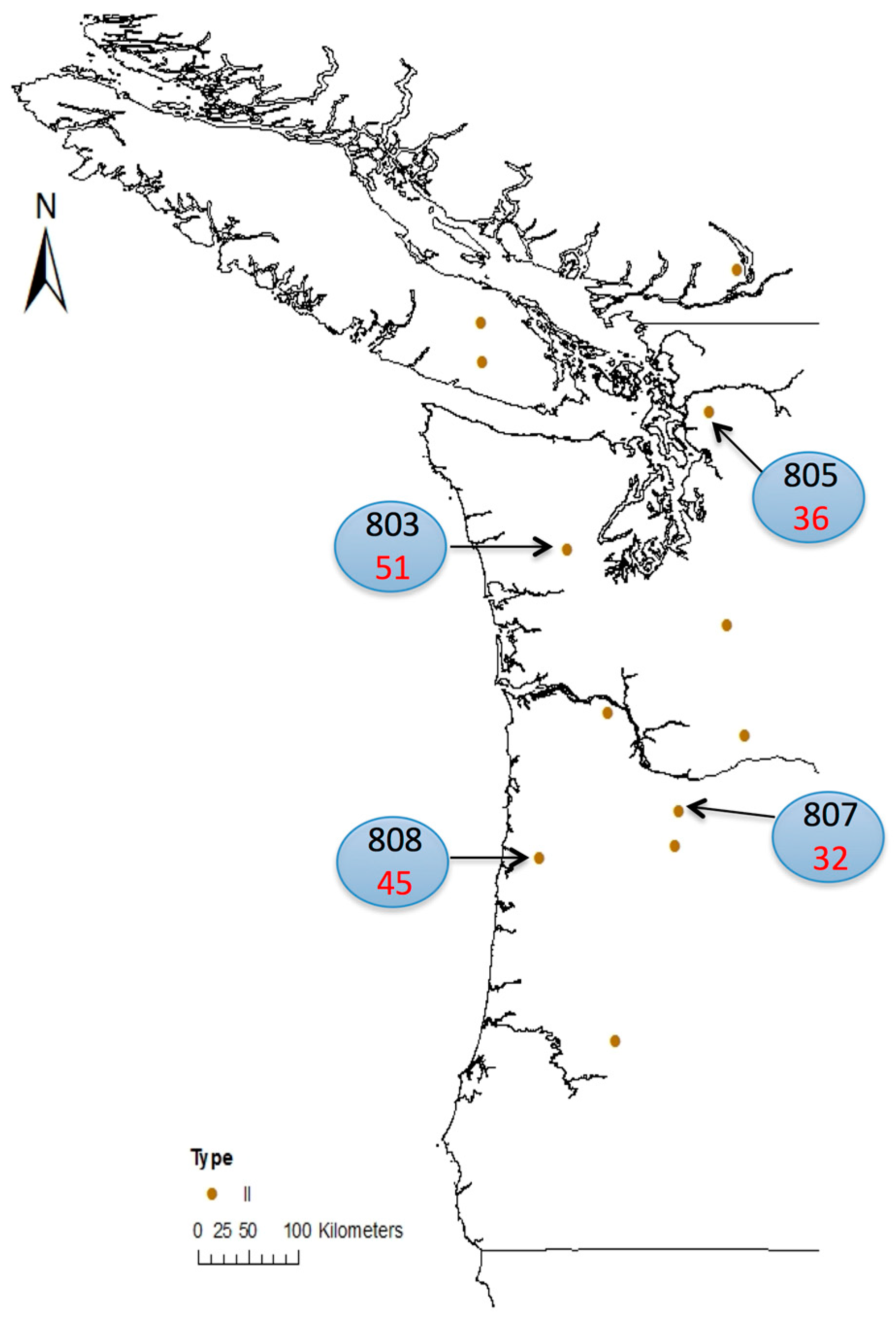
The Stand Management Cooperative (SMC), based at the University of Washington, established long-term research installations designed to address the effects of forest management regimes and silvicultural treatments on stand and tree growth and development. The SMC Type II installations were designed to provide data representative of plantations reaching a commercial thinning stage of development at the time of study establishment [38]. In 2006, these installations had reached the end of their designed measurement cycle and land owners were free to harvest them. Four of these installations (numbered 803, 805, 807, and 808) representing a wide geographic range and two rotation age levels (third and fifth decades) were selected for this study (Figure 1) in order to assess the relationship between lumber quality and stand/tree/log variables and to assess the effects of thinning on lumber stiffness at rotation (final harvest).

Each installation contained five plots (0.4 ha) representing different thinning regimes (

Table 1. Thinning regime, Relative Density triggers, and thinning dates (with corresponding stand ages) with the last row containing the rotation ages (final harvest ages in years since planting) for each installation. Study trees came from the final harvest.

Treatment Code	Thinning Regime	RD a Trigger Sequence	Installation Thinning Dates (Age at Thinning)
			803	805	807	808
A	No thinning (Control)		none	none	none	none
B	Thin heavy once	RD55-RD30;	1987	1990	1989	1991
		no further thinning	(33)	(21)	(15)	(31)
C	Delayed thinning	RD65-RD35; no further thinning	none	none	1993 (19)	1993 (33)
D	Repeated, heavy thinning	RD55-RD30; subsequent thinnings RD50-RD30	1987 (33)	1990 (21) 2004 (34)	1989 (15) 2001 (30)	1993 (33)
E	Repeated,	RD55-RD35;	1987(33)	1996(27)	1989(15)	1991(31)
	light thinning	RD55-RD40; subsequent thinnings RD60-RD40
	Rotation age	(Final harvest age)	51	36	45	32

^a RD = relative density [39].

) all harvested in the same calendar year (2006) to provide the material for this study. Thinnings were triggered (implemented) when the stand attained a particular value of Curtis’ [39] stand relative density (RD). Curtis’ relative density measures the extent that trees have captured available growing space. In the case of Douglas-fir, stands that have a measured RD lower than ~15 are essentially open-grown.

Stands in which the RD is between ~15 to 30 are growing large individual trees rapidly, but generally at the expense of per hectare production. Stands that have a measured RD between 30 and 55 may have slower individual tree growth rates but are still increasing the per hectare production with increases in RD. Whereas stands beyond an RD of 55 are beginning to lose stems due to competition-induced mortality though the individual tree size continues to increase as does the per hectare yield. Generally speaking, for the objective of producing wood volume, one strategy is to commercially thin either once or several times to earn income during a rotation, which serves at the same time to maintain or enhance tree and stand growth rates after thinning. If multiple thinnings are contemplated, a general strategy is to thin less frequently and more lightly as the stand ages. For example, the thinning regime behind treatment code D allows a stand to just reach the imminent competition-induced mortality boundary and thins back nearly to a condition where the per hectare production may be sacrificed; subsequent thinnings maintain an overall lower density stand condition by keeping the RD no higher than 50.

Site, stand, and average tree characteristics by treated plot at the age when harvested appear in

Table 2. Selected site, stand and tree characteristics for the four installations by plot.

Inst. (elev, m)	Plot	SI a	Density	BA b	QMD c	Ht	Avg Stem Taper	LCR d	LLAD Butt Log e
(slope, %)		m@50y	trees/ha	m2/ha	cm	m	cm/m	%	cm
803	A	36	791	56	30.0	36.6	1.05	30	2.54
(585)	B	37	306	45	43.4	39.0	1.12	37	2.54
(1)	C	35	899	52	26.9	35.1	0.97	29	1.78
	D	35	336	45	41.4	35.4	1.17	33	3.30
	E	34	459	47	36.1	33.8	1.05	30	1.78
805	A	38	860	52	27.7	30.8	0.94	36	4.57
(168)	B	40	454	40	33.5	31.4	1.03	37	3.05
(15)	C	39	366	33	34.0	32.3	1.00	41	4.32
	D	41	420	42	35.6	32.0	1.24	39	2.79
	E	39	405	36	33.8	32.3	1.12	39	5.33
807	A	33	1398	49	21.1	24.1	1.13	27	1.27
(152)	B	33	741	39	25.9	24.7	1.12	34	2.03
(1)	C	30	825	36	23.4	23.2	1.12	37	2.54
	D	35	395	27	29.2	25.9	1.17	43	3.05
	E	37	929	40	23.4	27.1	1.05	33	0.76
808	A	34	731	62	32.8	31.1	1.28	37	2.03
(762)	B	33	296	44	43.4	30.9	1.42	47	2.79
(5)	C	-	-	-	-	-	-	-	-
	D	31	247	42	46.7	28.7	1.57	51	2.29
	E	33	351	50	42.4	30.8	1.46	39	3.05

^a SI = site index; ^b BA = basal area; ^c QMD = quadratic mean diameter; ^d LCR = live crown ratio; ^e LLAD = largest limb average diameter in first 4.9 m (16 ft).

. The delayed thinning plot (C) of installation 808 was lost due to a windstorm, so no data were available for this treatment from that site.

2.2. Tree, Log, and Lumber Measurements

As there is a relationship among the NDT values of trees, logs, and lumber [34], TreeSonic velocity (TSV) was measured on the standing tree at breast-height as time-of-flight (nanoseconds) of an acoustic wave over a 1 m distance using the Fakopp TreeSonic instrument on 50 plot-centered trees on each of the plots. Mill trial trees were selected based on the distribution of the TSV. Twelve trees were selected from each plot. Two, four, four, and two trees from each plot were randomly selected from the following four TSV categories: The lowest 10%, medium-low 11–50%, medium-high 51–90%, and the top 10%, respectively for processing into lumber and veneer. Six trees were randomly chosen using the above TSV distribution and allocated to the lumber recovery study. The lumber recovery trees were bucked into 10 m (33 ft) logs in the woods, delivered to the South Union Sawmill in Elma, WA, and cut into 4.9 m (16 ft) logs in the log yard. From each tree, the resonant acoustic velocity of the merchantable bole and the 10 m (33 ft) length logs was measured in the woods, and the 4.9 m (16 ft) logs were measured at the sawmill using the Director HM200 [34]. Logs were processed into predominantly 5.1 × 10.2 cm (2 × 4 in) and 5.1 × 15.2 cm (2 × 6 in) lumber. Most of the MSR and MEL lumber produced were of these sizes. In addition, the location and size of the largest knot in each quadrant of the 4.9 m (16 ft) log segments were measured to calculate the large limb average diameter (LLAD) also known as branch index (BIX). The location and size of any ramicorn branches were also recorded.

Logs were sawn using a Mighty Mite circular saw (7.1 mm or 0.28 in saw kerf) with horizontal edger blades. Each piece of lumber was labeled to identify the tree and log it came from as well as the log position within the tree. The lumber was kiln-dried and surfaced. Finished lumber was visually graded by a certified lumber grader from the Western Wood Products Association and grade-limiting defects were recorded for each piece. All lumber was shipped to the USDA Forest Products Laboratory (FPL), Madison, WI for MOE determination using the MetriGuard e-computer. All data were collected from fall 2006 through spring 2007.

The MOE was adjusted to 15% moisture content [40] to calculate the volume-weighted log MOE. The percentage of lumber that met the MSR/MEL grade requirements was calculated based on the moisture content adjusted MOE.

2.3. Data Analysis

First, the branch index, grade-limiting defect, and lumber stiffness were summarized by the stand and silviculture regime. Next, the lumber grade distributions among the silviculture regimes and MOE distributions by lumber grade were examined more rigorously through an explanatory modeling effort. One set of equations was developed to assess the effects of site, stand, tree and log attributes on the proportion of log volume by visual lumber grade and another set of equations generated to assess how the same attributes affect the proportion of lumber volume that meets the structural design specifications for each grade. Each set of equations was developed using a two-step process.

The proportion of log volume in a visual grade was modeled first. In the first step, a model was developed to predict the presence of a grade within a log. The presence was indicated with a one (1), absence with a zero (0). In the second step, the abundance of the grade was estimated given that the grade was present. Although on the surface our data contained what appeared to be a very large number of observed zeroes, which indicate the absence of a grade within a log, methods to account for such a condition [41] showed no improvement to the fit when the model was recast as a fractional regression. Therefore, a generalized linear mixed-effects model was chosen to describe the presence of a grade, linked to a logistic error distribution, which maximized the likelihood of the parameters when the response is Bernoulli. The model appears in Equation (1).

$$p=\frac{1}{\left(1+e^{-\left({\mathsf{\beta }}_0+b_{0i}+{\mathsf{\beta }}_1{X}_1+{\mathsf{\beta }}_2{X}_2+\dots \right)}\right)}+{\mathsf{\delta }}_i$$

(1)

where p denotes presence (p = 1) or absence (p = 0) of a grade within a log, e denotes the base of the natural logarithm, Xs denote the set of predictor variables examined, βs are the fixed model coefficients, b_0i are random deviations due to the plot from the fixed component of the model coefficient, β₀, and δ_i are random error terms describing the residual variation unexplained by the predictor variables and random plot effects.

In the second step, an abundance model to predict the proportion of log volume in a particular visual grade given its presence was developed using a linear mixed-effects regression model. Since the proportion of a particular grade within a log is, by definition, any number between zero (0) and one (1), the log odds-ratio transformation (logit) was applied to the observed response values to normalize their distribution. The model form appears in Equation (2).

$$logit\left(\mathsf{\theta }\right)={\mathsf{\beta }}_0+b_{0i}+{\mathsf{\beta }}_1{X}_1+{\mathsf{\beta }}_2{X}_2+\dots e_i$$

(2)

where θ denotes the proportion of log volume in one of the grades, logit(θ) denotes the natural logarithm of the ratio of the proportion in the grade to the proportion that is not, or “log odds-ratio”, X_is denote the set of predictor variables examined, β_is are fixed model coefficients, b_0i is the random deviation due to the plot from the fixed component of the model coefficient, β₀, and e_i are the random error terms describing the residual variation unexplained by the predictor variables and random plot effects.

The design values were assigned [42] to meet the engineering requirements of the intended end use of the lumber (structural capability). They differ not only by end use but also by species and are influenced by such features as knots and slope of grain. The size of lumber was also a consideration in assigning design value. Structural lumber (including dimension lumber) can be visually and/or mechanically (MSR) graded for its strength and physical working properties. The set of models, derived to estimate the proportion of lumber volume meeting the structural design values for Douglas-fir, were derived similarly to the visual grade models.

In the first step, a model was derived to predict the presence of lumber meeting the structural value within a grade using the same model as Equation (1), while the second step model estimated the proportion of volume meeting the structural design value given that it was present using the same model as Equation (2). A two-step modeling process, such as used here, has previously been used quite successfully in other contexts where the conceptual framework is analogous (see for example Reference [43]).

Installation, or geographic location, effects were accounted for as fixed effects in the models in the form of site attributes, such as slope, aspect, elevation, among others. The effects of the plot were considered random in all fitted models, to assess and characterize the magnitude of uncontrollable noise, i.e., variation that is unaccounted for by the treatments applied. The only exceptions to this were the Economy visual grade and No. 3 structural grade abundance models, each of which lacked a sufficiently large sample size to assess the plot variation adequately. Thinning methods were expected to express their influences in the form of differing stand density, basal area, and average stand diameter that were attained over the course of time through stand dynamics processes as moderated by silvicultural thinning. Tree variables (Diameter at Breast Height [DBH] total height, taper, height-diameter ratio) were considered to be fixed, measurable effects. Each model set was developed using a forward selection of variables, with a chosen significance level of 0.1 for all models. Given the high level of variation observed among plots and trees, this less conservative significance level was chosen in order to capture all important variables influencing the presence and abundance of the grades. Twenty candidate predictor variables were evaluated for each model including treatment (silviculture regime and harvest age), site (latitude, longitude, slope, aspect, and elevation), plot (Trees Per Hectare [TPH], Quadratic Mean Diameter [QMD], basal area, relative density, site index), tree (DBH, height, height-DBH ratio, taper, and acoustic velocity), and log (small-end diameter, position along the stem, and LLAD) attributes. Only main effects were considered. The lme4 R package was used for fitting the models [44].

For binary presence/absence models, methods to assess the fit in a meaningful way are not well defined, which also holds true for logit models, or models where proportions represent the response. We chose the following method for evaluating the overall combined fit for the two-model sets. After fitting the models, the mean predicted abundance for each grade was determined using a Monte Carlo simulation. In this process, a random number between zero and one was generated 500 times per grade for each log in the dataset and compared to the modeled probability of presence. The abundance was then tallied as either the predicted abundance when the random number did not exceed the modeled presence probability or zero otherwise. The results were averaged to calculate the mean response per grade for each log. Finally, the predicted abundance for all grades within a log was scaled proportionally to sum to one. The set of equations were evaluated as a system by comparing these predictions to the observed values by calculating the following set of fit statistics: The adjusted R-squared, root mean squared error, mean absolute deviation, mean bias, and mean percent error.

3. Results

3.1. Initial Data Summary

A total of 1758 pieces of lumber were sawn from 317 logs out of 97 trees. The reduced number of trees from the 112 trees originally selected was primarily due to weather conditions on installation 807 (13 trees were not transported to the mill) and the inability to saw the remaining four trees due to defects (sweep) and size (log small-end scaling diameter). About 25% of the lumber produced was 5.1 × 10.2 cm (2 × 4 in) and the remaining 75% was 5.1 × 15.2 cm (2 × 6 in). A very small amount of 2.5 cm (1 in) lumber was sawn. Restricting the lumber sizes allowed for a better assessment of the impact of knots on the lumber grade. The yield of No. 2 and better (a grade grouping often found in marketing Douglas-fir) lumber ranged from 91 to 95%.

Table 3. Sample data and percent volume yield by lumber grade of the sampled installations.

Inst.	Age	Tree	DBH	Height	Logs Processed	Lumber Pieces	Lumber Grade
	yr	n	cm	m	n	n			pct
							Sel Str a	No. 1	No. 2	No. 3	Econ b
803	51	29	39.11	35.97	119	718	29	40	26	4	1
805	36	27	35.05	31.70	77	368	23	44	29	3	2
807	32	17	28.70	24.69	33	119	7	35	49	6	3
808	45	24	43.43	30.18	88	553	23	37	31	7	2
Total		97			317	1758

^a Sel Str = select structural lumber grade; ^b Econ = economy lumber grade.

shows the lumber data and grade yield from the study.

3.1.1. Branch Index

Another of the main factors directly affecting the lumber grade is the size of knots, which start as branches on the tree. The branch index (LLAD) on the bottom 4.9 m (16 ft) log ranged from a low of 1.8 cm (0.7 in) to a high of 5.3 cm (2.1 in). Douglas-fir is not prone to self-pruning dead branches below the live crown [22]. Thus, thinning that impacts the crown structure can impact knot type and size. The butt log typically contains the highest value lumber.

3.1.2. Grade-Limiting Defect

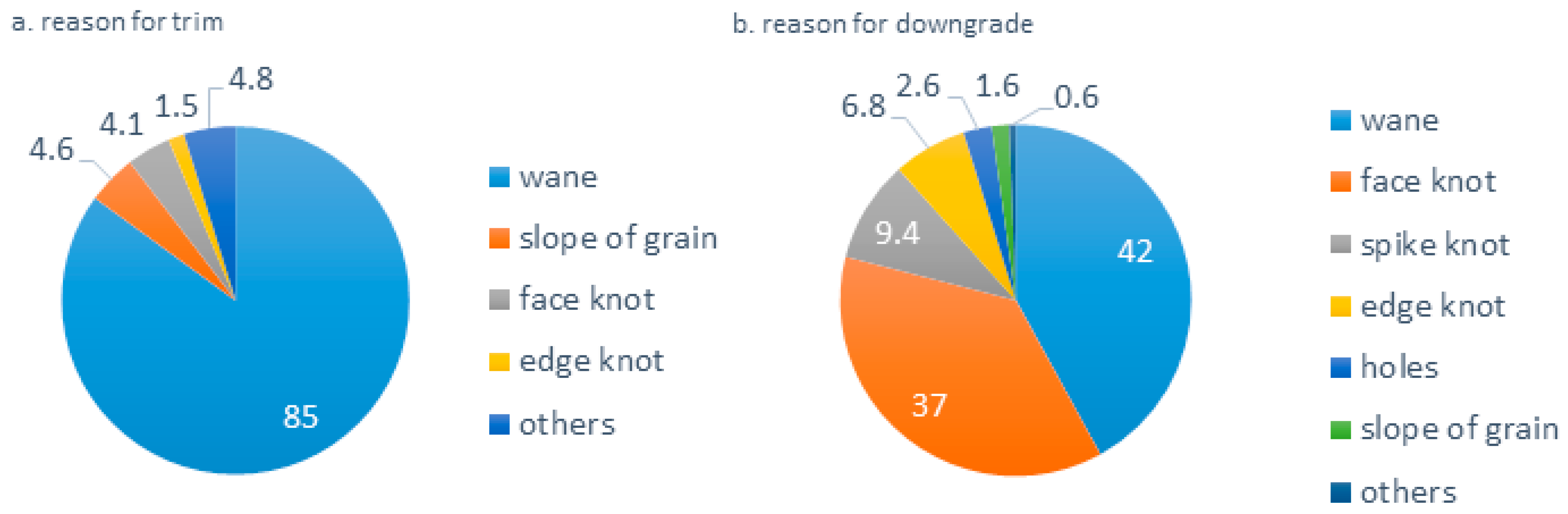
Wane (85%) and knots (6%) were the dominant reasons for trimming lumber (about 190 pieces or 11%) to increase the grade (Figure 2a). These were also the two factors that were the grade-limiting defects, causing the lumber to be downgraded (Figure 2b). Intensive management can increase taper in a tree, especially in the upper stem, that leads to the presence of wane in lumber. Forty-two percent of the lumber was downgraded for wane. Face knots (the primary grade-limiting knot type) accounted for 37% of the downgrade. Spike and edge knots accounted for an additional 16% of the downgrade.

3.1.3. Lumber Stiffness

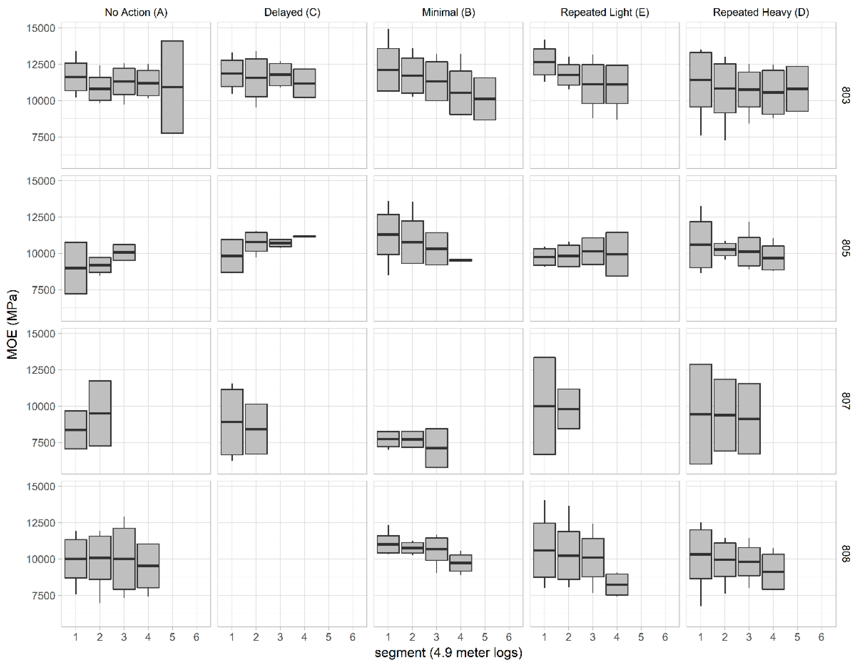
The volume-weighted MOE by log position of the tested installations is shown in Figure 3. The MOE exhibits gradients from the tree base to the tree top, being more variable in the younger stands (805 and 808). The log lumber MOE is related to other variables besides log diameter and log position, including juvenile wood proportion and wood density. Upper segments near the top of the tree (e.g., segment 4) generally have a higher proportion of juvenile wood and a lower wood density.

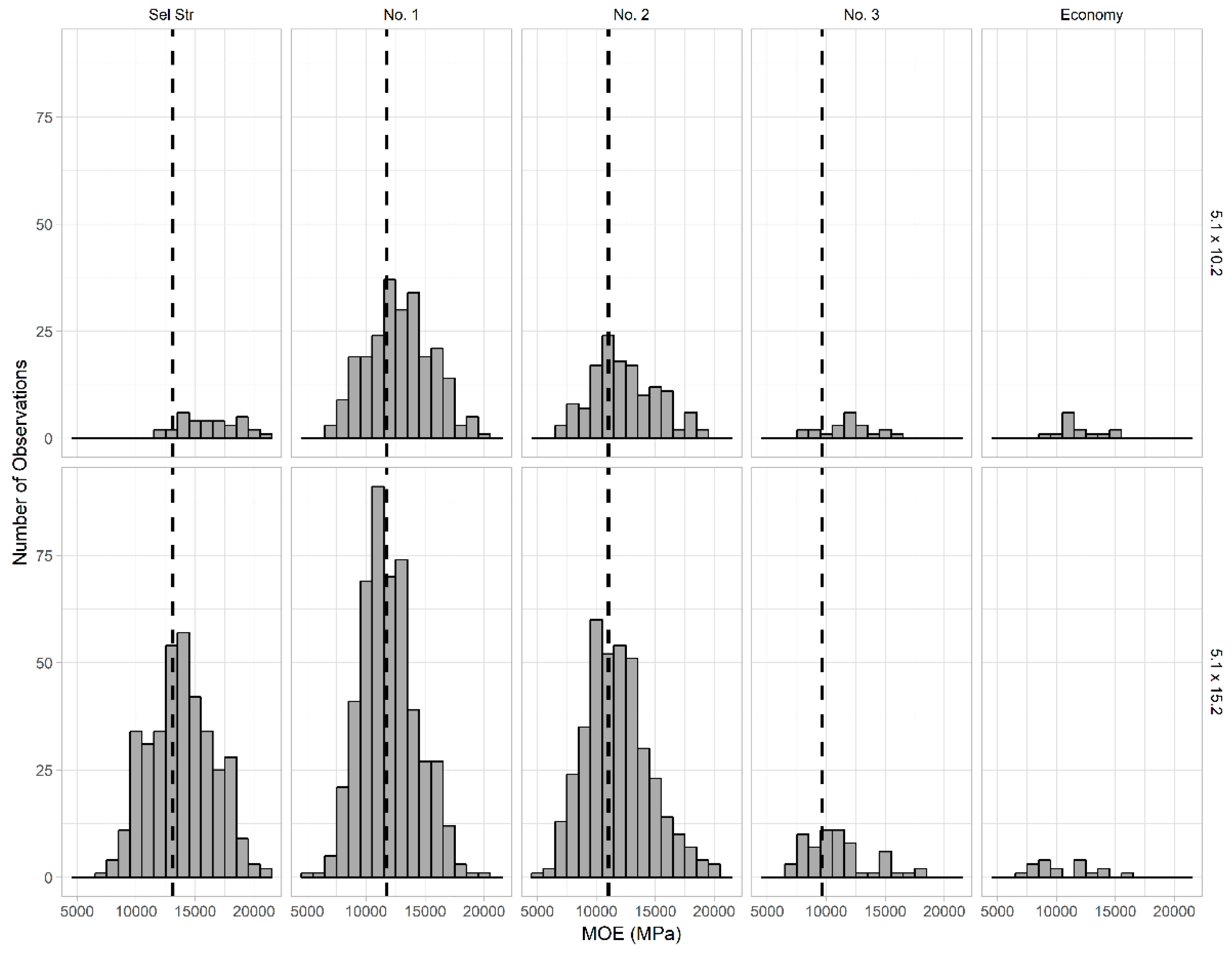
The percentage of Douglas-fir visual grade lumber that meets the design value is related to the amount of juvenile wood [13]. In this study, about 50% of the visually graded lumber met or exceeded the design value [26] (Figure 4). Of note is the small sample size of No. 3 grade lumber and the number of 5.1 × 10.2 cm (2 × 4 in) lumber that met the Select Structural grade.

Except for installation 803, the higher grades of the tested plantation lumber had average MOE values that fell below the published MOE design values (

Table 4. Average density (weighted by lumber volume) and lumber MOE by site and visual grade (number in parentheses is MOE design value of the grade).

Site	Density	MOE	Sel Str (13,100)	No. 1 (11,721)	No. 2 (11,032)	No. 3 (9653)	Econ
	(kg/m3)	MPa
803	569	13,334	14,162 ^	12,473 *	12,638 *	12,555 **	12,052
805	551	11,625	12,114	11,438	11,052 ^	10,587 **	11,101
807	521	10,004	11,749	9694	9894	11,018 *	10,949
808	580	11,521	13,017	11,321	10,839	9218	10,018

^ MOE average meets the specification but its distribution does not; * MOE average meets MEL; ** MSR meets MOE specifications (the amount of below-grade MOE pieces is more lenient for MEL grading rules).

).

The calculations used to derive the proportions meeting the design values relied only on the MOE limit, so if additional design limits were incorporated in those calculations, the amounts of below-grade lumber will probably be larger. One interesting observation of the test results is that when compared to pine species, the MOE of the lower visual grade Douglas-fir lumber was relatively high, which may be explained by the intrinsic stiffness property of Douglas-fir. There were many high MOE pieces within the visual grade plantation-grown lumber that keep the average MOE of the grade on par, but the amount of low MOE lumber in the distribution can fail the grading rules. The cause of the additional low MOE pieces could most likely be due to the increased proportion of juvenile wood within the log.

3.2. Modeling Summary

3.2.1. Lumber Grade Distribution

In the first step, the presence/absence of each grade within a log was modeled. This resulted in the selected predictor variables listed in

Table 5. Selected parameters and level of significance for lumber visual grade presence/absence models.

Variable	Sel Str	No. 1	No. 2	No. 3	Econ
Intercept	−3.4227 **	0.1283	1.4725	−4.6907 ***	−5.9568 ***
Plot QMD	0.0926 *		−0.0539 *
Tree DBH				0.0943 ***
Tree height			−0.1158 **
Tree taper	−4.3120 ***
Log SED	0.2006 ***	0.0707 *	0.1554 ***		0.1007 **
Log LLAD			0.1194 **
Log position				−1.6142 *
${\sigma }_{b_0}^2$	0.4847	0.0789	0.0097	0.0958	0.9674

Significance level symbols ***, **, and * indicate p-value ranges of p < 0.001, 0.001 < p < 0.01, and 0.01 < p < 0.05, respectively. Intercept terms were always included regardless of significance to maintain unbiasedness.

showing the coefficient estimates and significance. Intercepts were kept in all models, even if not significant, so that models remain unbiased and would at minimum be capable of predicting a mean presence value, in cases where there may be no significant tree or stand variables.

In the second step, the abundance of each grade within a log, given that it was present, was modeled. This resulted in the selected predictor variables listed in

Table 6. Selected parameters and level of significance for the lumber visual grade abundance models.

Variable	Sel Str	No. 1	No. 2	No. 3	Econ
Intercept	5.7471 **	1.9021	−1.1781 +	−0.1635	1.620
Installation slope		0.0985 +
Plot TPA			0.0009 *
Plot QMD	0.0491 +
Plot site index	−0.1135 *	−0.1440 **
Tree DBH	−0.0481 *
Tree height		0.0994 ***
Tree taper	−1.6227 +		1.3858 **
Tree velocity		7.7888 *
Log SED		−0.1264 ***	−0.0593 ***	−0.0384 *	−0.2373 +
Log LLAD			0.0773 *
${\sigma }_{b_0}^2$	0.0661	0.0097	0.0132	0.0058	NA
${\sigma }_e^2$	1.4872	1.6036	1.3930	0.4116	1.8578

Significance level symbols ***, **, *, and ⁺ indicate p-value ranges of p < 0.001, 0.001 < p < 0.01, 0.01 < p < 0.05, and 0.05 < p < 0.1, respectively. Intercept terms were always included regardless of significance to maintain unbiasedness.

, showing the coefficient estimates and level of significance. Here as well, intercepts were kept in all models, even if not significant, so that models remain unbiased and will at minimum be capable of predicting a mean abundance value, in cases where there may be no significant tree or stand variables.

As stated in the methods section, each set of equations was evaluated as a system by comparing the Monte Carlo predicted values to the observed values. Summary statistics were calculated based on 1575 data points (315 logs × 5 lumber grades) and 34 parameters (

Table 7. Summary of the fit statistics for the final lumber visual grade model system.

Statistic	Value
Adjusted R-squared	0.4279
Root Mean Squared Error	0.2015
Mean Absolute Deviation	0.1409
Mean Bias	2.4939 × 10−18
Mean Percent Error	0.7045

).

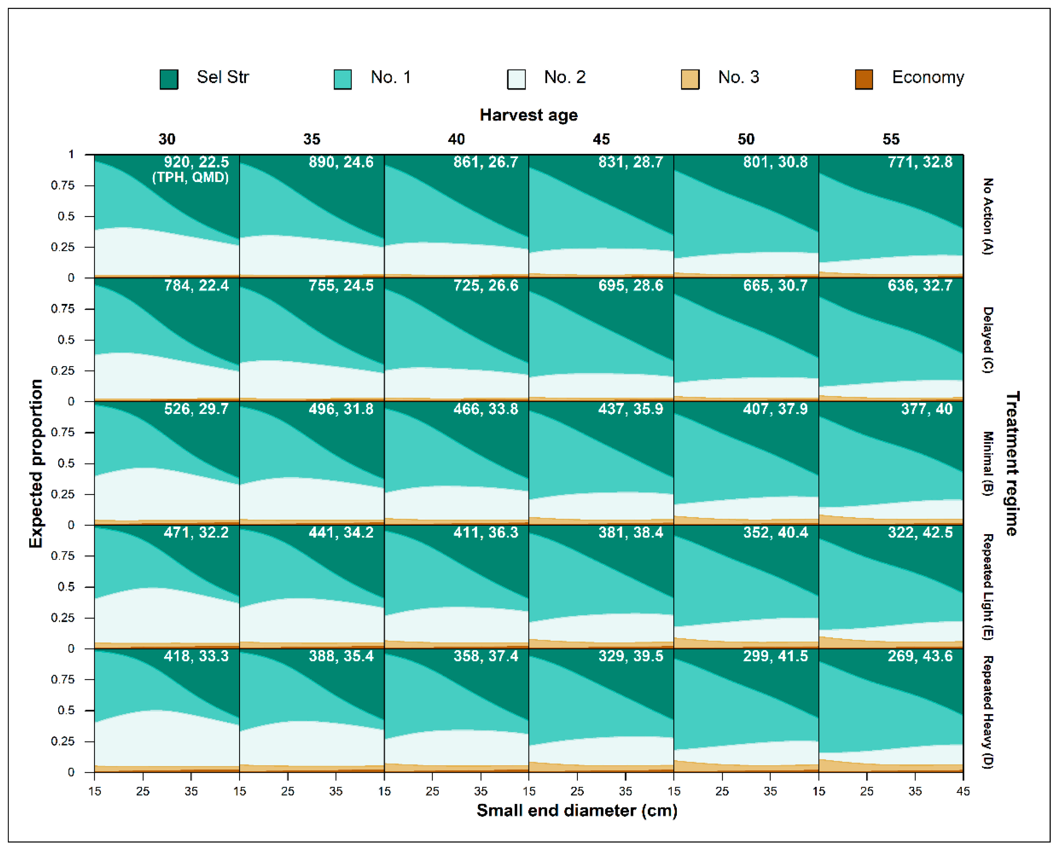
The behaviors of the visual grade models as a system were explored by comparing the effects of log small-end diameter (SED), harvest age, and treatment regime on the predicted grade proportions. To accomplish this, linear regression models were first developed to predict model input parameters, including TPH, QMD, tree height, and LLAD, from harvest age and treatment regime. Harvest ages were chosen to range from 30 to 55 years by 5-year steps. The log SED values were chosen to range from 10.2 to 45.7 cm (6 to 18 in) by 7.6 cm (3 in) steps. The log position parameter was chosen to be 0.25, representing the butt log of the tree. The remaining parameters were set to median values for the data set. The results are illustrated in Figure 5.

Log SED and harvest age have the largest effects on the model. As the small-end diameter of a log increases, the proportion of the Select Structural grade increases at the expense of the No. 1 grade, while No. 2 and the remaining grades stay relatively flat. For a given harvest age, grade No. 2 has a positive relationship with the log SED at its low end but turns negative for larger SEDs. Increasing the harvest age results in proportionally larger amounts of Select Structural in the lower SED range, but proportionally smaller amounts in the larger SEDs. Proportionally more No. 1 grade was produced over all SEDs as the harvest age increased. The No. 2 grade decreases proportionally over the range of the SED with harvest age, while No. 3 and Economy (E) were predicted in very small proportions in all scenarios.

The thinning regime appears to have a much smaller effect on the distribution of grade, for reasons stated previously. Grades Select Structural and No. 1 occurred in slightly larger proportions in a smaller diameter, denser stands for a given harvest age and small end diameter. These results may differ for absolute abundance, as logs with larger small-end diameters would be expected to occur more frequently in stands with a lower density (fewer trees per hectare that are larger in diameter for a given harvest age). This system of models provides a methodology to better understand the influences of silvicultural thinning on the tree and stand attributes that can be used directly to predict the proportion of lumber grades to expect under the different regimes. This will lead to greater accuracy and precision when appraising/valuing the resultant products produced.

3.2.2. Lumber Structural Grade

The proportion of lumber volume for a visual grade that met the MOE standard was calculated for each log. For presence/absence modeling purposes, presence was defined as any proportion greater than zero that met the MOE standard for a particular grade. Economy grade does not have a structural design standard. The selected variables and estimates of the coefficients are reported in

Table 8. Selected parameters and level of significance for lumber structural grade presence/absence models.

Variable	Sel Str	No. 1	No. 2	No. 3
Intercept	−10.2863 **	−3.5808 ***	−4.1380 **	−29.5200 *
Harvest age	0.0997 **	0.0642 **
Tree height			0.2028 ***
Tree velocity	21.5060 *			83.0200 *
Log position	−3.0699 **		−2.1948 **
Log SED		0.0642 **
${\sigma }_{b_0}^2$	0.0629	0.0770	0.1012	3.5360

Significance level symbols ***, **, *, and ⁺ indicate p-value ranges of p < 0.001, 0.001 < p < 0.01, 0.01 < p < 0.05, and 0.05 < p < 0.1, respectively. Intercept terms were always included regardless of significance to maintain unbiasedness.

and

Table 9. Selected parameters and level of significance for lumber structural grade abundance models.

Variable	Sel Str	No. 1	No. 2	No. 3
Intercept	−6.4760 +	−4.9053 +	7.7580 ***	9.495 ***
Tree velocity	22.7280 **	16.6633 *
Tree taper			−3.6568 ***	−4.2934 ***
Log LLAD			−0.1663 *
${\sigma }_{b_0}^2$	0.2970	9.142 × 10−16	4.113 × 10−16	NA
${\sigma }_e^2$	4.4090	4.7690	4.3180	1.9061

Significance level symbols ***, **, *, and ⁺ indicate p-value ranges of p < 0.001, 0.001 < p < 0.01, 0.01 < p < 0.05, and 0.05 < p < 0.1, respectively. Intercept terms were always included regardless of significance to maintain unbiasedness.

for the presence/absence and abundance models, respectively.

Overall, the structural grade models explained a very low amount of variation in the response variables. Summary statistics are reported in

Table 10. Summary of the fit statistics for the two-equation structural grade model sets by visual grade.

Statistic	Sel Str	No. 1	No. 2	No. 3
Adjusted R-squared	0.1533	0.0407	0.1405	0.3649
Root Mean Squared Error	0.3714	0.3804	0.3821	0.3092
Mean Absolute Deviation	0.3269	0.3320	0.3403	0.2153
Mean Bias	−1.601 × 10−17	2.0497 × 10−17	−5.7301 × 10−19	−4.8720 × 10−18
Mean Percent Error	0.4631	0.5559	0.4952	0.2539

.

4. Discussion

The data themselves are highly variable, leading to somewhat low R-squared values in all models, but the main objective, again, was assessing the significance of factor effects to explain the responses, not necessarily creating a model with a high precision for predictive use; though that remains an outcome to be desired and eventually achieved. It should be noted that although treatment regime variables were actually tested throughout in all the models, they were always supplanted by the actual stand and tree attributes at final harvest. This does not mean that treatments were ineffective in producing differences in log and lumber grades, only that treatment affects themselves appear indirectly through their accumulated impact over the rotation on the responses by way of their influence on stand dynamics processes [19,45].

Considering first the lumber visual grade presence model (Table 5), it is seen that the greatest single impact on a single grade is tree taper. Logically, as taper increases, the presence of the Sel Str grade is less likely. The single predictor that had influence over most of the grades was the small-end diameter of the log (log SED) variable. This is completely expected since this is the main driving variable in the visual log grading system that is used in the Pacific Northwest [46]. Log small-end diameter was most influential in the select structural lumber grade (largest coefficient), but it will be seen that a large diameter log benefits the presence of all grades (positive signs). The average diameter of the stand (plot QMD) positively influenced the presence of the Select Structural grade, as expected, further enhancing the positive effect of the log SED. For the Select Structural grade, a greater degree of taper negatively influenced its presence, likely due to less solid central wood in the log that is capable of producing higher grade lumber, i.e., a larger proportion of wood in jacket boards (lumber sawn from the outer portion of a log), slabs and edgings. The presence of the No. 2 grade was negatively impacted by stands with an overall larger plot QMD, and especially so if the tree was among the taller component. Though a large Tree DBH will help the probability that the No. 3 grade is present, it will be less likely in the upper logs. The Economy grade presence seems insensitive to all other stand and tree attributes, perhaps because it captures all the lumber not in the other grades.

When considering the abundance of visual grades, given their presence, we see again that log small-end diameter was the most important variable overall (Table 6), because it remained significant in four of the five grade models, which no other predictor variable did. Though the coefficients were all negative, we can interpret the magnitudes of the coefficients as indicating tradeoffs in lumber volume between grades. For example, a log with a large SED may produce all grades of lumber, but will produce the most Select Structural lumber (coefficient is zero, i.e., no negative impact from the SED), followed by No. 3 (smallest magnitude negative coefficient), then, No. 2 (next larger magnitude coefficient), No. 1 (even larger negative coefficient), and finally Economy (largest negative coefficient), respectively. The next overall most important variable might be considered to be either the plot site index or tree taper. A higher site index decreases the Select Structural and No. 1 grades, likely due to fewer rings per inch in the logs produced since the site index has been shown to be reflected visibly in rings per inch, the two variables being essentially interchangeable [47]. A greater tree taper negatively impacts the Select Structural grade, which seems to be offset by more No. 2 grade, another tradeoff. The slope of the ground at the site (installation slope) positively impacted the abundance of No. 1 grade lumber. This result was somewhat unexpected, and while further exploration of why this might be important is beyond the scope of this study, it is interesting to speculate how this and other environmental attributes or climatic variables may influence tree growth, wood production and subsequent lumber grade turnout; currently under investigation elsewhere [48]. Overall, stands with a larger average diameter produced relatively more Select Structural lumber, though it was tempered by individual tree DBH; its abundance was decreased to a greater degree if the tree had a DBH larger than QMD. As expected, grade No. 2 tolerates larger knots (LLAD) [26]. The net effect of high-density stands is to produce trees with less taper and seems to positively influence the abundance of No. 2 grade lumber. The magnitude of between-plot variation for the visual grade abundance models was quite small compared to residual error.

For the structural grade models (Table 8 and Table 9), log position (inversely related to log diameter) or log SED were chosen for the Select Structural, No. 1, and No. 2 grades. Log diameter has been correlated to lumber grade recovery and thus value [27]. Harvest age and TSV (Tree Velocity) were each selected for multiple models. The presence of the Select Structural and No. 1 grades showed positive relationships with harvest age. This might be expected since as trees age, annual ring widths tend to become narrower, even if the growth rate doesn’t slow because the annual wood layer would be laid down on an ever increasing diameter. This, in turn, would lead to an increased density in the outer rings (higher proportion of LW), leading to a greater stiffness. The tree velocity (TSV) showed a positive relationship with the response variables, also as expected, because the speed of an acoustic wave through wood is directly and positively correlated with wood stiffness; an important structural attribute [34]. The Select Structural and No. 1 grades of lumber were more likely to be present in larger diameter logs (occurring lower in the tree) harvested from older stands, as expected. The presence of No. 2 grade was more likely in logs from taller trees located lower in the bole. No. 3 grade presence was predicted by only the Tree velocity. The Economy grade is known not to yield any structural lumber, so there is no design value assigned to it.

The structural abundance models (Table 9), largely exhibited variables with signs that were easily interpreted. As expected, the greater the TSV, the greater the abundance of the Select Structural and No. 1 grades, given that they were present. Given the presence of the No. 2 and 3 grades, a greater tree taper reduced abundance. The abundance of the No. 2 grade was further negatively impacted when the LLAD was large, likely due to grain distortion around the knots. Fahey [14] also found that the LLAD influenced lumber grade recovery in Douglas-fir. The magnitude of plot-to-plot variation for the structural grade abundance models was relatively small compared to residual error.

Both sets of models for both the visual grade presence and abundance and presence and abundance of structural lumber within a grade clearly demonstrated that visual lumber grade alone is insufficient for predicting the actual quantity of lumber produced that meets the structural design values for each grade. The incorporation of other tree and stand variables, resulting from stand treatment, into the models helped the prediction of visual lumber grades more so than for structural lumber, as judged by the fit statistics evaluated (Table 7 and Table 10).

5. Conclusions

Decision support tools need to be integrated at every step in the value chain, from stand management to log marketing. For a lumber mill, the amount of high MOE material is enough to satisfy the current small MSR/MEL market and the visual grade lumber is the main product. Therefore, the effects of low MOE wood on Douglas-fir lumber mills are relatively small as long as the majority of the lumber meets the visual specifications. On the other hand, the MOE is directly related to the value of engineered wood products (EWP), so for manufacturers producing EWP, the additional low MOE materials directly reduce mill profit. Not only does having surplus low MOE material cause waste in an EWP facility, but additional high MOE materials need to be purchased on the open market to fill customer orders. Unlike visually graded lumber, the internal strength and stiffness are the key value factors of EWP. Balancing the MOE in a log mix for EWP mills is getting more complicated with the increasing amount of low MOE juvenile wood in the wood basket.

The use of non-destructive, in-woods testing equipment to measure acoustic velocity was found to be the most important variable for predicting the presence of structural grades in the lumber produced.

The MOE is but one factor among other considerations in making various types of timberland investment and forest management decisions. Plantation forests are a long-term investment and knowledge gained from operational research, such as a mill trial, enables tree growers to tailor their prescriptions to meet customer needs and allocate logs for maximum profit. A clear understanding of the internal quality of standing timber provides flexibility for landowners to capture established and emerging markets and for manufacturers to meet product specifications, adapt to changing grading rules, and develop new products. Such knowledge is necessary to gain a market share and price advantage. Internal wood quality sorting technologies are necessary for log suppliers to deliver the right log to the right mill; however, the vendors may not have a sufficient understanding in operation constraints for developing cost-effective tools for the timberlands and the mills. Logs account for 50–70% of the operational cost of a mill, and a consistent and reliable supply of log mix is a necessity for mill managers. For some reason, communication barriers are frequently found between mills and log suppliers. The disappearance of vertically integrated forest companies makes the information sharing even more difficult.

References

- Barbour, R.J.; Kellogg, R.M. Forest management and end-product quality: A Canadian perspective. Can. J. For. Res. 1990, 20, 405–414. [Google Scholar] [CrossRef]
- Vance, E.D.; Maguire, D.A.; Zalesney, R.S., Jr. Research Strategies for Increasing Productivity of Intensively Managed Forest Plantations. J. For. 2010, 108, 183–192. [Google Scholar]
- Cherry, M.; Vikas, V.; Briggs, D.; Cress, D.W.; Howe, G.T. Genetic variation in direct and indirect measures of wood stiffness in coastal Douglas-fir. Can. J. For. Res. 2008, 38, 2476–2486. [Google Scholar] [CrossRef]
- Vikram, V.; Cherry, M.L.; Briggs, D.; Cress, D.W.; Evans, R.; Howe, G.T. Stiffness of Douglas-fir lumber: Effects of wood properties and genetics. Can. J. For. Res. 2011, 41, 1160–1173. [Google Scholar] [CrossRef]
- Jozsa, L.A.; Middleton, G.R. A Discussion of Wood Quality Attributes and Their Practical Implications, SP-34; Forintek Canada Corp.: Vancouver, BC, Canada, 1994. [Google Scholar]
- Kennedy, R.W. Coniferous wood quality in the future: Concerns and strategies. Wood Sci. Technol. 1995, 29, 321–338. [Google Scholar] [CrossRef]
- Gartner, B.L. Assessing wood characteristics and wood quality in intensively managed plantations. J. For. 2005, 103, 75–77. [Google Scholar]
- Megraw, R. Douglas-fir Wood Properties. In Douglas-Fir: Stand Management for the Future; Oliver, C.D., Hanley, D.P., Johnson, J.A., Eds.; College of Forest Resources, University of Washington: Seattle, WA, USA, 1986; pp. 81–96. [Google Scholar]
- Abdel-Gadir, A.Y.; Krahmer, R.L. Estimating the age of demarcation of juvenile and mature wood in Douglas-fir. Wood Fiber Sci. 2007, 25, 242–249. [Google Scholar]
- Aubry, C.A.; Adams, W.T.; Fahey, T.D. Determination of relative economic weights for multitrait selection in coastal Douglas-fir. Can. J. For. Res. 1998, 28, 1164–1170. [Google Scholar] [CrossRef]
- Kellogg, R.M. Second Growth Douglas-Fir: Its Management and Conversion for Value, SP-32; Forintek Canada Corp.: Vancouver, BC, Canada, 1989. [Google Scholar]
- Barratt, J.D.; Kellogg, R.M. Lumber Quality from second growth managed forests. In A Technical Workshop: Juvenile Wood–What Does It Mean to Forest Management and Forest Products? Forest Products Research Society: Madison, WI, USA, 1986; pp. 57–71. [Google Scholar]
- Barrett, J.D.; Kellogg, R.M. Strength and Stiffness of Dimension Lumber. In Second Growth Douglas-Fir; Its Management and Conversion for Value, Special Publ. SP-32; Kellogg, R.M., Ed.; Forintek Canada Corp.: Vancouver, BC, Canada, 1989; pp. 50–58. [Google Scholar]
- Fahey, T.D.; Cahill, J.M.; Snellgrove, T.A.; Heath, L.S. Lumber and Veneer Recovery from Intensively Managed Young-Growth Douglas-Fir; US Department of Agriculture, Forest Service: Portland, OR, USA, 1991.
- Bendtsen, B.A.; Plantinga, P.L.; Snellgrove, T.A. The influence of juvenile wood on the mechanical properties of 2 by 4’s cut from Douglas-fir plantations. In Proceedings of the International Conference on Timber Engineering, Pullman, WA, USA, 19–22 September 1988; Washington State Univ.: Pullman, WA, USA, 1988; pp. 226–240. [Google Scholar]
- Lowell, E.C.; Maguire, D.A.; Briggs, D.G.; Turnblom, E.C.; Jayawickrama, K.J.; Bryce, J. Effects of silviculture and genetics on branch/knot attributes of coastal Pacific Northwest Douglas-fir and implications for wood quality—A Synthesis. Forests 2014, 5, 1717–1736. [Google Scholar] [CrossRef]
- Curtis, R.O.; Reukema, D.L. Crown development and site estimates in a Douglas-fir plantation spacing test. For. Sci. 1970, 16, 287–301. [Google Scholar]
- Grah, R.F. Relationship between tree spacing, knot size, and log quality in young Douglas-fir stands. J. For. 1961, 59, 270–272. [Google Scholar]
- Weiskittel, A.R.; Maguire, D.A.; Monserud, R.A.; Rose, R.; Turnblom, E.C. Intensive management influence on Douglas fir stem form, branch characteristics, and simulated product recovery. N. Z. J. For. Sci. 2006, 36, 293–312. [Google Scholar]
- Brix, H. Effects of thinning and nitrogen fertilization on branch and foliage production in Douglas-fir. Can. J. For. Res. 1981, 11, 502–511. [Google Scholar] [CrossRef]
- Maguire, D.A.; Kershaw, J.A., Jr.; Hann, D.W. Predicting the effects of silvicultural regime on branch size and crown wood core in Douglas-fir. For. Sci. 1991, 37, 1409–1428. [Google Scholar]
- Maguire, D.A.; Johnston, S.R.; Cahill, J. Predicting branch diameters on second-growth Douglas-fir from tree-level descriptors. Can. J. For. Res. 1999, 29, 1829–1840. [Google Scholar] [CrossRef]
- Briggs, D.G.; Kantavichai, R.; Turnblom, E.C. Predicting the diameter of the largest breast-height region branch of Douglas-fir trees in thinned and fertilized plantations. For. Prod. J. 2010, 60, 322–330. [Google Scholar] [CrossRef]
- Reukema, D.L. Crown expansion and stem radial growth of Douglas-fir as influenced by release. For. Sci. 1964, 10, 192–199. [Google Scholar]
- Barbour, R.J.; Parry, D.L. Log and Lumber Grades as Indicators of Wood Quality in 20- to 100-Year Old Douglas-Fir Trees from Thinned and Unthinned Stands; US Department of Agriculture, Forest Service: Portland, OR, USA, 2001.
- Western Wood Products Association (WWPA). Western Lumber Grading Rules; Western Wood Products Association: Portland, OR, USA, 2017. [Google Scholar]
- Middleton, G.R.; Munro, B.D. Log and Lumber Yields. In Second Growth Douglas-Fir: Its Management and Conversion for Value; Kellogg, R.M., Ed.; Forintek Canada Corp.: Vancouver, BC, Canada, 1989; Chapter 7; pp. 66–74. [Google Scholar]
- Briggs, D.G.; Ingaramo, L.; Turnblom, E.C. Number and Diameter of Breast-height Region Branches in a Douglas-fir Spacing Trial and Linkage to Log Quality. For. Prod. J. 2007, 57, 28–34. [Google Scholar]
- Ross, R.J.; McDonald, K.A.; Green, D.W.; Schad, K. Relationship between log and lumber modulus of elasticity. For. Prod. J. 1997, 47, 89–92. [Google Scholar]
- Ross, R.J.; Willits, S.A.; VonSegen, W.; Black, T.; Brashaw, B.K.; Pellerin, R.F. A stress wave based approach to NDE of logs for assessing potential veneer quality. Part I. Small diameter ponderosa pine. For. Prod. J. 1999, 49, 60–62. [Google Scholar]
- Ridoutt, B.G.; Wealleans, K.R.; Booker, R.E.; McConchie, D.L.; Ball, R.D. Comparison of log segregation methods for structural lumber yield improvement. For. Prod. J. 1999, 49, 63–66. [Google Scholar]
- Carter, P.; Briggs, D.; Ross, R.J.; Wang, X. Acoustic testing to enhance western forest values and meet customer wood quality needs. In Productivity of Western Forests: A Forest Products Focus; Harrington, C.A., Schoenholz, S.H., Eds.; US Department of Agriculture Forest Service: Portland, OR, USA, 2005; pp. 121–129. [Google Scholar]
- Wang, X.; Ross, R.J.; McClellan, M.; Barbour, R.J.; Erickson, J.R.; Forsman, J.W.; McGinnis, G.D. Nondestructive evaluation of standing trees with a stress wave method. Wood Fiber Sci. 2001, 33, 522–533. [Google Scholar]
- Wang, X.; Carter, P.; Ross, R.J.; Brashaw, B.K. Acoustic assessment of wood quality of raw forest materials—A path to increased profitability. For. Prod. J. 2007, 57, 6–14. [Google Scholar]
- Wang, X.; Ross, R.J.; Carter, P. Acoustic evaluation of wood in standing trees. Part I. Acoustic wave behavior. Wood Fiber Sci. 2007, 39, 28–38. [Google Scholar]
- Amishev, D.; Murphy, G.E. In-forest assessment of veneer grade Douglas-fir logs based on acoustic measurement of wood stiffness. For. Prod. J. 2008, 58, 42–47. [Google Scholar]
- Briggs, D.G.; Thienel, G.; Turnblom, E.C.; Lowell, E.; Dykstra, D.; Ross, R.J.; Wang, X.; Carter, P. Influence of thinning on acoustic velocity of Douglas-fir trees in western Washington and western Oregon. In Proceedings of the 15th International Symposium on Nondestructive Testing of Wood, Duluth, MN, USA, 10–12 September 2007; pp. 113–123. [Google Scholar]
- Maguire, D.A.; Bennett, W.S.; Kershaw, J.A., Jr.; Gonyea, R.; Chappell, H.N. Establishment Report Stand Management Cooperative Project Field Installations, Institute of Forest Resources Contrib. 72; College of Forest Resources, University of Washington: Seattle, WA, USA, 1991. [Google Scholar]
- Curtis, R.O. A simple index of stand density for Douglas-fir. For. Sci. 1982, 28, 92–94. [Google Scholar]
- Evans, J.W.; Kretschmann, D.E.; Herian, V.L.; Green, D.W. Procedures for Developing Allowable Properties for a Single Species Under ASTM1900 and Computer Programs Useful for the Calculation; US Department of Agriculture, Forest Service: Madison, WI, USA, 2001.
- Ramalho, E.A.; Ramalho, J.J.; Murteira, J.M. Alternative estimating and testing empirical strategies for fractional regression models. J. Econ. Surv. 2011, 25, 19–68. [Google Scholar] [CrossRef]
- American Forest and Paper Association/American Wood Council (AF & PA/AWC). Wood Structural Design Data; American Forest and Paper Association: Washington, DC, USA, 2004. [Google Scholar]
- Zhao, D.; Borders, B.; Wang, M. Survival model for fusiform rust infected loblolly pine plantations with and without mid-rotation understory vegetation control. For. Ecol. Manag. 2006, 235, 232–239. [Google Scholar] [CrossRef]
- Bates, D.; Maechler, M.; Bolker, B.; Walker, S.; Christensen, R.H.B.; Singmann, H.; Dai, B.; Scheipl, F.; Grothendieck, G.; Green, P. Linear Mixed-Effects Models Using ‘Eigen’ and S4: Package ‘lme4’. 2018. Available online: https://cran.r-project.org/web/packages/lme4/lme4.pdf (accessed on 19 February 2018).
- Oliver, C.D.; Larson, B.C. Forest Stand Dynamics; Update Edition; Wiley: New York, NY, USA, 1996; 520p. [Google Scholar]
- Northwest Log Rules Advisory Group. Official Rules for the Following Log Scaling and Grading Bureaus: Columbia River, Grays Harbor, Northern California, Puget Sound, Southern Oregon, Yamhill; Northwest Log Rules Advisory Group: Eugene, OR, USA, 1998; 48p. [Google Scholar]
- Hoibo, O.A.; Turnblom, E.C. Models of knot characteristics in young coastal U.S. Douglas-fir: Are the effects of tree and site data visibly rendered in the annual ring width pattern at breast height? For. Prod. J. 2017, 67, 29–38. [Google Scholar]
- Todoroki, C.L.; Lowell, E.C.; Kantavichai, R. Growth and mortality in response to climatic extremes and competition in thinning trials of Douglas-fir. manuscript in preparation.
Figure 1.
Locations of the Stand Management Cooperative (SMC) installations selected for this study. The numbers in red are the rotation ages of the stands when harvested.
Figure 2.
Percent of end-trim of lumber (a) and visual grade downgrade factors (b) for all lumber combined.
Figure 3.
Log lumber MOE by segment (log position within the tree with the butt log being segment 1) and thinning type by installation. Note: Segments are 4.9 m logs (16 ft logs).
Figure 4.
Distribution of lumber MOE by lumber size and visual grades. The dotted vertical line is the published MOE value for the specific grade. Economy lumber does not have a structural design value assigned to it.
Figure 5.
Expected proportion of log volume by lumber visual grade by harvest age, treatment regime, and log small end diameter. Trees per hectare (TPH) and quadratic mean diameter (QMD) for each rotation age by treatment panel are shown in the upper right corner.