What Makes a UI Simple? Difficulty and Complexity in Tasks Engaging Visual-Spatial Working Memory


1
Automated Control Systems Department, Novosibirsk State Technical University, 630073 Novosibirsk, Russia
2
Psychology and Pedagogy Department, Novosibirsk State Technical University, 630073 Novosibirsk, Russia
*
Author to whom correspondence should be addressed.
Future Internet 2021, 13(1), 21; https://0-doi-org.brum.beds.ac.uk/10.3390/fi13010021
Submission received: 22 December 2020
/
Revised: 15 January 2021
/
Accepted: 16 January 2021
/
Published: 19 January 2021
(This article belongs to the Special Issue VR, AR, and 3-D User Interfaces for Measurement and Control)
Abstract
:Tasks that imply engagement of visual-spatial working memory (VSWM) are common in interaction with two-dimensional graphical user interfaces. In our paper, we consider two groups of factors as predictors of user performance in such tasks: (1) the metrics based on compression algorithms (RLE and Deflate) plus the Hick’s law, which are known to be characteristic of visual complexity, and (2) metrics based on Gestalt groping principle of proximity, operationalized as von Neumann and Moore range 1 neighborhoods from the cellular automata theory. We involved 88 subjects who performed about 5000 VSWM-engaging tasks and 78 participants who assessed the complexity of the tasks’ configurations. We found that the Gestalt-based predictors had a notable advantage over the visual complexity-based ones, as the memorized chunks best corresponded to von Neumann neighborhood groping. The latter was further used in the formulation of index of difficulty and throughput for VSWM-engaging tasks, which we proposed by analogy with the infamous Fitts’ law. In our experimental study, throughput amounted to 3.75 bit/s, and we believe that it can be utilized for comparing and assessing UI designs.
1. Introduction
The growing diversity of devices and contexts in which users interact with online resources is leading to the advent of the so-called Big Interaction. With it, custom “hand-made” design and testing of user interfaces (UIs) are increasingly supported or even substituted with computer-aided automated approaches. Already it is argued [1] that the main prerequisite for designing human–computer UIs of adequate quality is our ability to formalize and model user behavior: cognitive processes (memory, attention, learning) [2], decision-making [3], performance in selection tasks, etc. Predictive models of user behavior, particularly if they concern features that designers can affect and tasks that are widespread in real interactions, are recognized as an efficient way of encapsulating knowledge and a sound basis for design tools [2]. Particularly, researchers call for more extensive usage of mathematical cognitive models that are currently “under-exploited” in HCI [4] (p. 2), and [2]. Today’s trend in such models is consideration of utility for subjects [4] or cost-benefit trade-offs [5], e.g., the ones optimizing the “expenditure” of perceptual-motor plus cognitive resources [6]. Among other things, they can predict the time spent by users in tasks of various difficulties so that the verification of UIs can be carried out without studies with the actual users [2,4].
One of the popular factors for behavior models is visual complexity (VC), which can act as a proxy for various HCI-related parameters, like aesthetic impression, which is considered highly important for the overall positive user experience [7]. The baseline metric for VC of most types of visual objects is produced by a compression algorithm, such as JPEG (as specified e.g., in ISO/IEC 10918-1:1994 standard), which was specifically designed to consider particulars of images perception by humans. Some alternatives include calculating Subband Entropy [8] or Fractal Dimension of the image, using Zipf’s Law, preliminary edge detection filters application, etc. [9]. In HCI and UI analysis, the above approaches have been successfully applied to images, textual content (characters recognition in fonts, graphic complexity [10], etc.), high-order UI design measures (e.g., amount of whitespace in [11]), and so on.
In our own previous work [12], we examined the user-subjective visual complexity of UI layouts, predicting it with objective metrics based on compression algorithms. An obvious argument for limited applicability of the VC factor for the models in HCI is its static nature and the resulting detachment from the actual user interaction with UI. On the other hand, VC is known to affect cognitive load [13], which is an essential component in the interaction efficiency and thus for UI usability. Although there are publications in other fields (e.g., cartography [14] or driving [15]) that study the effect of VC beyond first impression and attractiveness perception, this kind of research in HCI is comparatively scarce. Therefore, in our work, we address the interaction tasks that engage the users’ visual-spatial working memory, which are prominent in modern graphic and web UIs. The study is motivated by the need for quantitative expressions of such tasks’ difficulty for the users, which could be further employed in automated assessment of UIs based on models of user behavior.
In interaction with today’s computer systems, a human primarily perceives information via the visual channel, while his or her information output is carried out through engagement of the motor system. In this interaction, the key element is working memory, particularly its visual-spatial short-term component, whose performance is also known to be an important index of intelligence and successful adaptation [16]. In relation to HCI, it reflects personal abilities in perception, storage, and designation of information, which are central for more sophisticated cognitive tasks in interaction: search, problem solving, activities planning, navigation in virtual space, etc. [17].
In psychology, there is still no ultimately clear distinction for the notions of “short-term memory” and “working memory” [18,19], as both functional purpose and temporal storage timeframe depend on the kind of information and the processing method. Working memory has been conceived and defined in three different, slightly discrepant ways: as short-term memory applied to cognitive tasks, as a multi-component system that holds and manipulates information in short-term memory, and as the use of attention to manage short-term memory [18] (p. 323). The short-term memory is generally opposed to the long-term one, as capacity and storage time of the former are limited, unlike the latter. Traditionally, the short-term memory capacity in sequential information presentation experiments (for letters, digits, words, images) was assessed as 7 ± 2 information units (items or “chunks”) by Miller and his co-authors—exceeding it would significantly worsen accuracy of the memorization. More recent results from [20,21], where objects with varying color, shape, and spatial location were presented to the subjects, suggest the limitation of 3–4 units. In the latter experiments, the stimuli were presented for quite a short time, which in our opinion makes information structuring volatile, and probably has less ecological validity with respect to HCI-related tasks. Although distinction between working memory and short-term memory is far from clear, the specific function of working memory refers to holding complex span tasks [19]. All in all, the working memory capabilities are rather dynamically shaped and affected by the nature of the presented material, its organization, context, and the cognitive load [22,23].
The visual-spatial information processing is considered a key component in working memory [24], which is reinforced by the numerous visual attention models existing in HCI [25]. The amount and spatial organization of the visualized information are the main factors of interest, as the corresponding results have clear implications for 2D UIs design and user performance prediction. Particularly, quite a large body of research work has shown that groping of visual elements does increase working memory performance [26,27,28].
Thus, in our paper, we study the factors influencing human performance in tasks that require engagement of visual-spatial working memory (VSWM) and inquire what the memorized information items (chunks) are. On the other hand, we can use the concept of working memory (VSWM) to refer to the maintenance plus manipulation of visual information while its reproduction by motor reaction. Particularly, we explored whether the popular characteristic of visual complexity, and its objective metrics based on compression algorithms can be used as an adequate predictor. As an alternative, we considered the metrics based on a simpler Gestalt groping principle of proximity, operationalized as von Neumann and Moore neighborhoods from the cellular automata theory. To that end, we undertook experimental sessions with the total of 164 subjects who performed about 5000 VSWM-related tasks and assessed visual complexity of their configurations.
The findings and contributions of our studies, further detailed in the Conclusions, are as follows:
- visual complexity and its metrics are rather weakly related to the accuracy in VSWM-related tasks,
- the strongest regularity used for grouping is best described with von Neumann range 1 neighborhood rule,
- the index of difficulty and throughput measure for the tasks engaging VSWM can be formulated as inspired by Fitts’ law,
- the throughput of 3.75 bit/s that we obtained in the experiment is consistent with the estimated range of 2–4 bit/s for memory-engaging tasks known from the literature.
2. Methods and Related Work
In the current section, we refine the research methodology and overview the work related to the information processing and complexity. We focus on the applications in HCI, without going into the underlying neurophysiologic and psychological mechanisms—more detailed info on Hick’s law can be found e.g., in [29], on Fitts’ law in [30], and the consideration of the laws’ practical applicability in [31]. In the final part of the section, we describe the experimental study that we undertook to validate our reasoning.
2.1. Information Theory-Based Measures
The enormous effect of Information Theory rapidly caused attempts to apply Shannon’s approaches to describe human behavior. One of the regularities in cognitive psychology that stood the test of time was proposed in 1952 and was subsequently named Hick’s law:
where RT is reaction time when choosing from equally probable alternatives, N is the number of alternatives, and b is a constant that Hick named the rate of gain of information. When proposing the final formulation for his model, Hick noted that it corresponds to the number of steps in hierarchical sequence of binary classification decisions [23]—hence the logarithm to the base two. Indeed, today we have convincing evidence that human information processing is based on binary search (dichotomies).
Further, the generalization of (1) to non-equiprobable alternatives was proposed by R. Hyman:
where H is the entropy (information quantity) of the stimuli set, aH and bH are empirically defined coefficients.
Another akin regularity, inspired by the Shannon-Hartley theorem on maximum transmission rate in a noisy channel, was put forward in 1954 and consolidated as Fitts’ law:
where MT is time needed to perform a rapid aimed movement to a target, A is movement distance, W is size of the target, a and b are coefficients usually found from regression. Fitts’ goal was to calculate the “transmission rate” of human motor system, so he formulated the index of difficulty (ID) as can be seen in (3) and used it to express the index or performance (IP):
An important subsequent advance was introduction of the means to account for the movement accuracy: the “effective” index of difficulty (IDe). In each actual movement task performed, effective distance (Ae) can be calculated as the distance actually travelled. Effective target width (We) is the normalized area where movements for each particular combination of the independent variables terminate (details can be found e.g., in [30]). Thus, the classic Fitts’ model (7) with the IDe becomes:
This allowed obtaining the motor system throughput (TP) measure that has substituted Fitts’ IP and that is calculated with some experimental data as follows:
where P is the number of participants and M is the number of combinations for the independent variables (A and W) in the experiment. TP is an objective and full measure of both speed and accuracy in certain experimental conditions, independent of a particular task’s setup.
Of the two above regularities, Fitts’ law sees much wider usage in HCI, which is particularly due to high practicality of the throughput measure, which can be used to effectively compare different versions of UIs or interface devices. For instance, Fitts’ law studies that employ standardized methodology reported throughput values in the ranges 3.7–4.9 bit/s for mouse, 1.6–2.6 for joystick, 1.0–2.9 for trackball, etc. [30] (p. 784). On the contrary, applicability of Hick-Hyman’s law (2) is rather limited, since it is unclear how to calculate the information quantity in stimuli in most practical tasks [31]. Examples of successful applications of the law in HCI include design of specially organized menus [32], describing behavior in visual search [33,34] and perception of visual complexity [12]. Still, objective measurement of “cognitive throughput” remains much more complicated compared to the motor system’s one, as we detail in the next sub-section.
2.2. Human Information Processing
In the classical work on Hick’s law, the coefficient 1/b, essentially information processing speed in choice reaction tasks, was found to be equal to about 6.7 bit/s. This value can vary significantly due to characteristics of the subjects and the stimuli type [35]. The Human Processor model (MHP) that was introduced in the 1980s but remains influential till the present day details the information processing in several interlinked sub-systems [36]: perceptual, cognitive, and motor one (Figure 1).
MHP allows prediction of the time required to perform HCI-related tasks, e.g., with GOMS model, as the sum of the times in the involved sub-systems. However, these may differ significantly for various user groups, tasks, contexts, etc.: e.g., a cognitive processor cycle duration varies in the range of 25–170 ms. The experimental values for human information input (Rin) and output (Rout) speeds reported in different research publications are not entirely consistent, particularly since different information measurement units had been used and the experimental setup wasn’t always specified in enough detail to convert to a single unified unit.
Still, available sources seem to be in agreement that the upper limit of human vocal cords’ long-term information output is about Rout = 5 syllables/s, i.e., about 12.5 sounds/s for English (for other languages, this value may differ). For humans equipped with instruments or tools, the values are generally presented in bit/s or chars/s. Handwriting is limited at 3.5 chars/s, while average typing speed is about 6.7 chars/s, with 10 chars/s being the top record. In any case, maximum speed of human as information transmitter is estimated at 40 bit/s. The values for conscious information reception are only marginally higher: Rin for speaking comprehension is estimated at 3–4 words/s, for reading comprehension at 2.5 words/s or 18 bit/s, for reading aloud at 30 bit/s, for visual recognition of familiar letters and digits at 55 bit/s. Most sources agree that although Rin for reading reaches about 45 bit/s, the average capability of human visual perception in long-term operation is only around 8 bit/s [37].
The information processing speed can be enhanced using more complex [38] and multi-dimensional signals—e.g., size, brightness, and color, instead of just one varying facet. Another factor that is known to increase the speed is training, which is partially related to the fact that the operator can process information with various degrees of memory engagement. For tasks that do require considerable information exchange with the memory, the performance speed is reported to decrease by the order of magnitude, to about 2–4 bit/s [37]. The comparative analysis of numerous publications on working memory mechanisms presented in [37] (pp. 201–206), suggests that in most cases, information processing speed amounted to 3–5 units/s (sic!—not bits, but various units, such as figures). Similar quantitative estimations of human information processing capabilities and working memory performance can also be traced back to [39] or [40].
Overall, it is believed that the analytical information-theoretic paradigm that does not consider spatial structures is fundamentally limited in explaining human perception that is mostly top-down, i.e., focused on higher-order images and structures. An important advantage in the field was the development of Algorithmic Information Theory (AIT) in the 1980s that allowed bonding Information Theory with the integral Gestalt approach, which is focused on organization of visual sensory input into a percept [41].
2.3. Gestalt Principles of Perception and Algorithmic Complexity-Based Measures
Gestalt is a psychology school that emerged in Germany in the early 20th century from research in perception (primarily a visual one) and the ability of the human mind to organize individual elements into a large whole, “other than the sum of its parts”. Detailed review of the history, main points and the “decline” of the school in the 1960s can be found in [42], where the authors also note that, during the last 20 years, there has been a revival of interest towards Gestalt approaches. We believe it may be due to the increasing complexity of HCI that accompanies the development of the ubiquitous online environment, to the rapid development of computer vision technologies, and so on.
The central position in the Gestalt approach belonged to the law of Prägnanz, stating that human organizes the perceived information in a regular, ordered, symmetrical and simple way. Thus, the common essence of the Gestalt principles is decreasing the number of perceived information chunks (units) for more efficient information processing—the human ability obtained from both evolution of the species and from individual experience. The list of Gestalt principles of perception is somehow poorly organized, but they can be briefly summarized as the following [42]:
- “proximity”: objects that are placed nearby or in the same area (e.g., inside a frame) are perceived as a group;
- “similarity”: objects that are matching in color, size, behavior (e.g., movement direction or speed), etc. are perceived as a group;
- “good form” and “closure”: groups are perceived in such a way that the objects form more simple and familiar figures (e.g., cross as two intersecting lines, not as two adjoined angles; or separate dots and strokes as discontinuous drawing of a letter);
- the principles that relate to interaction between foreground and background.
It is known that the Gestalt principles are not equivalent in their effect on perception, but until now, no convincing structure describing the effects of individual principles and their combinations was proposed [43,44,45]. For example, objects allocated on a two-dimensional field may be groped either based on proximity or on good form, depending on the circumstances. Indeed, the Gestalt adherents proposed no unified formal theory, the fact that allowed critics to declare Gestalt to be merely descriptive and poorly suited for a deeper understanding of psychological and cognitive processes. However, AIT allowed directly linking the Gestalt’s concept of “simplicity” and the probability—the foundation of the Information Theory—thus uniting the two approaches. AIT implies coded representations of visual forms and states that the complexity of a percept is the length of the shortest string that generates the percept, thus basing itself on Kolmogorov’s algorithmic complexity [41]. Since the latter is incomputable, the lengths of the strings produced with compression algorithms often act as its practical approximation, and indeed it has been shown that the coded string lengths, the complexity measures, and performance measures in experiments are highly correlated [43].
In one of our previous works [12], we applied two classical lossless image compression algorithms, RLE [44] and Deflate [45], to describe visual complexity perception. The former algorithm replaces “runs” of data with a single data value and the count of how many times it’s repeated (see programming code of the implementation in Appendix A). The algorithm doesn’t deal with 2D images but can work with the linear string of bytes containing serialized rows of the image. Deflate is based on combination of LZ77 algorithm and Huffman coding: frequent symbols in the string are replaced with shorted representations, while rare symbols are coded with longer ones. The Huffman coding is now widespread, being used in compression of many kinds of data, especially photos (JPEG) and multimedia, as well as in data transmission protocols. To obtain the Deflate-compressed string length, we relied on PHP’s standard zlib_encode function, called with ZLIB_ENCODING_RAW parameter, corresponding to the RFC 1951 specification (please see [12] for a more detailed description of the implementation for both algorithms and the related AIT basis) (The online tool outputting the RLE and Deflate compressed string lengths for a given coded representation is available at http://www.wuikb.info/matrix/). Therefore, in the current study, we compare the predictive ability of the compressed strings’ lengths with the simpler metrics that basically only consider the proximity groping in the perceptual organization.
2.4. Von Neumann and Moore Neighbourhoods in Cellular Automata
Cellular automata (CA) are discrete dynamic models consisting of a regular grid of cells, each of which can be in a finite number of states σi,j:
where (i,j) are integer values representing the cells’ coordinates for a two-dimensional CA. In the simplest case, k equals 2, corresponding to the “off” (0) and “on” (1) states of the cell.
Another constituent of CA that make them useful for mathematical modeling of dynamic processes, are generations that start from the initial state (t = 0) and go onwards (advancing t by 1). The transitions between the generations are performed according to pre-specified rules for changing the states of the cells, generally based on the states of neighboring cells. In CA apparatus, there are two most common approaches for determining proximity:
- (1)
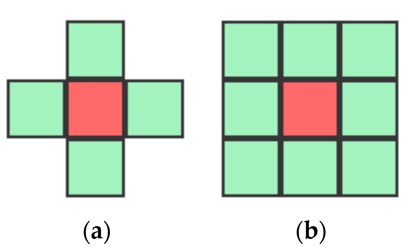
- Von Neumann neighborhood of range R is defined as:
- (2)
- Moore neighborhood of range R is defined as:
Figure 2 illustrates the two neighborhoods of range R = 1.
The maximum number of different transition rules (NR) for n neighbors and k possible states is then:
However, consideration of transitions in CA as interface models is beyond the scope of this paper, in which we consider only “static” complexity, i.e., corresponding to a 2-dimensional GUI screen. In the subsequent experiment, we calculate the number of “figures” that are formed from randomly positioned cells in “on” state (corresponding to interface elements) among cells in “off” state (corresponding to whitespace) in the cellular automation grid (The online tool that we developed for calculating the numbers of von Neumann and Moore figures is also available at http://www.wuikb.info/matrix/).
3. Experiment Description
In the first round of our experiment, the subjects performed memorization of graphical elements randomly positioned within 2D area. To constrain the number of factors in the experiment and to maintain similarity with CAs (7), we did not alter color, size, etc. of the elements, so the setup corresponded to k = 2, i.e., the basic CA with 0 and 1 states of cells. The preliminary results of the first round’s analysis were previously published in [46] (in Russian). In the second round, we collected subjective visual complexity evaluations for the same allocations (layouts) of the elements in the 2D area. To negate the effect of familiarity, we held it more than 1 year later, and mostly with different subjects. As we mentioned before, we previously published the results of our visual complexity investigation in [12], but there we did not consider the difficulty of the tasks engaging VSWM, which is the major focus of our current work.
In psychology, memorization performance is traditionally measured as accuracy, but for the purposes of HCI, we also consider the time on task. The latter is, however, unavoidably biased by the designation stage, so accuracy generally has the priority, even though the throughput measure that we ultimately propose encompasses both.
3.1. Goals and Hypotheses
The goal of our experiment was twofold: (1) to check if visual complexity and its compression-based measures characterize the difficulty of tasks engaging VSWM, or if proximity-based measures inspired by CA have an advantage, (2) to develop and validate objective performance measure for such tasks, in a fashion similar to Fitts’ throughput. The first goal would result foremost in contributions 1 and 2 as listed in the Conclusions, while the second one would be closely associated with contributions 3 and 4.
Reasoning about the formulation of the index of difficulty for VSWM-related tasks (IDM), we can assume that in visual-spatial perception tasks (visual search and memorization of objects), two components can be identified: informational and spatial. The former relates to information quantity of the “message” held in memory, while the latter relates to spatial allocation of its elements. Indeed, the widely accepted model is that the “what” and “where” information processing is performed in ventral and dorsal streams of the brain, respectively. Our assumption is also supported by [38], where performance in 2D objects selection tasks was best explained with the index of selection difficulty incorporating the number of objects and binary logarithm of their vocabulary size. In that study, the effect of the perceived area size combined with the two other factors was also significant, but the exact nature of their effects is seemingly task-dependent. That is, if the search runs through the memorized information, the performance will be affected by the logarithm of items in memory, such as e.g., images of friends in [47]. Correspondingly, if the search instead runs through some applicable spatial positions, the difficulty of such tasks should be characterized by the number of memorized items (NI) and the binary logarithm of the size of the considered area (S0), where the items can be located:
The proposed function (11) is based on the above reasoning and our assumptions, which are to be experimentally validated. Thus, we formulated the following hypotheses for the experiment:
- Performance in VSWM tasks is best predicted with the same compression-based factors as visual complexity.
- Performance in VSWM tasks is best predicted with the simpler proximity-based factors.
- Performance in VSWM tasks is best predicted with our proposed index of difficulty.
- The values calculated for the corresponding quantitative task setup-independent measure of performance that also encompasses time are consistent with the ones found in the literature.
3.2. Material and Procedure
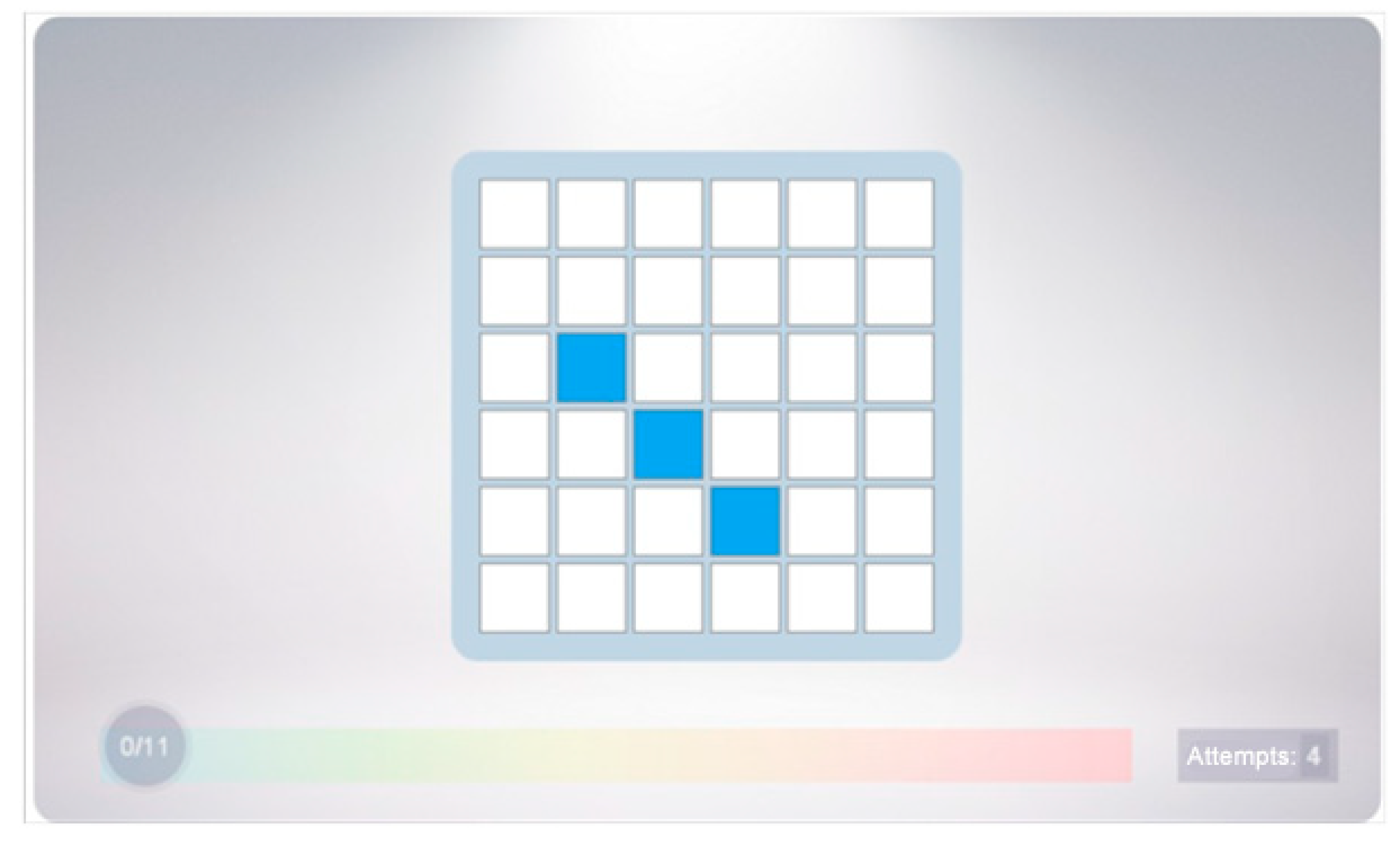
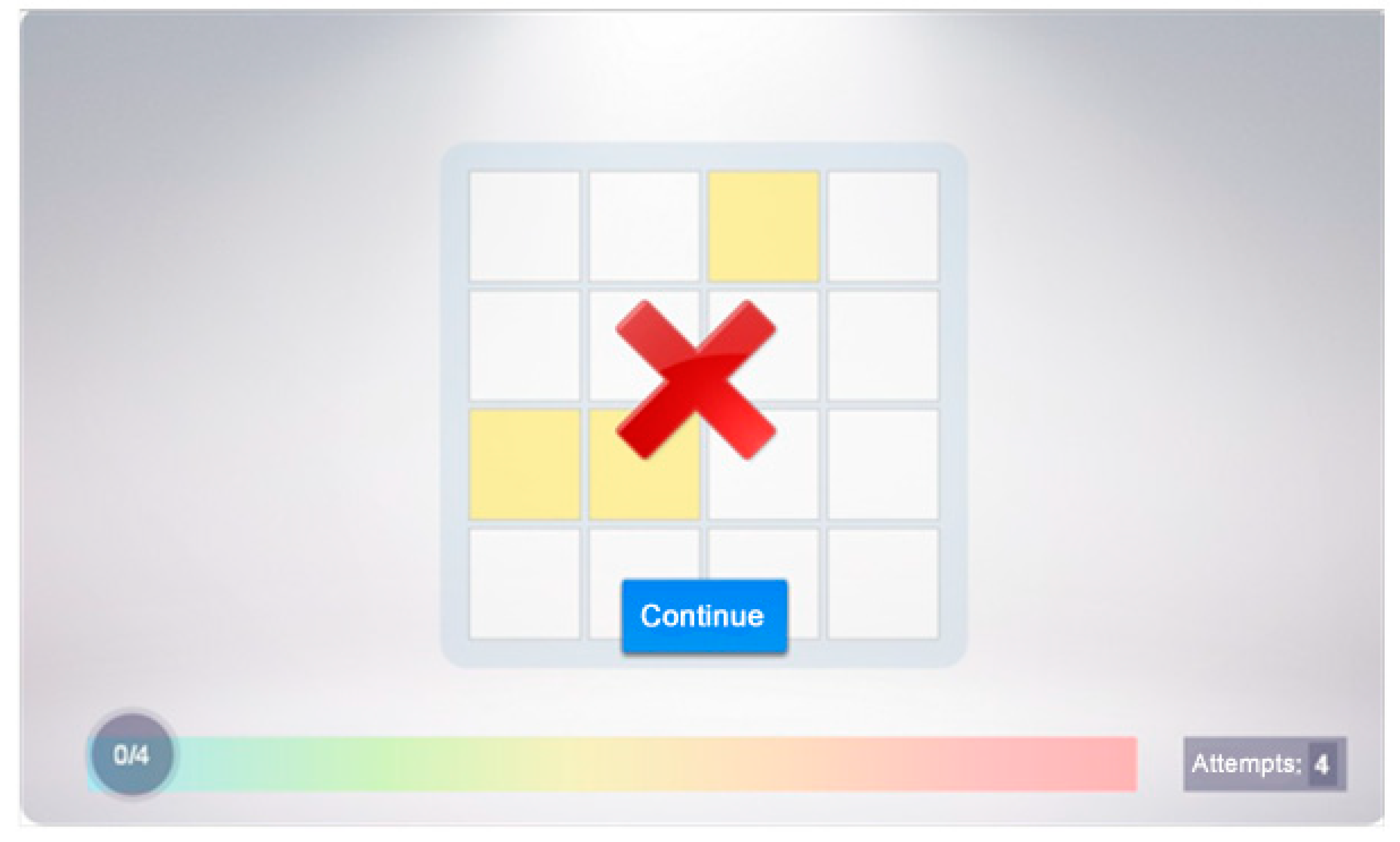
Each trial in the first round of the experiment would include the two stages, memorization, and designation. Such an approach is generally accepted in the field as Visual Patterns Test, and we believe that separation of the stages is virtually impossible when studying working memory in healthy people. In the memorization stage, the subject was shown square 2D area with grid lines that formed square cells, of which randomly selected ones were filled with blue color (Figure 3). We allowed a reasonably long time (2 s) for the stimuli presentation, unrelated of the number of the cells, so that our experimental setup corresponds to the classic works of Miller and co-authors. For the subsequent designation stage, all the cells would turn blank, and the participant needed to remember and click the ones that used to be filled. The correctly clicked cells would turn green, while incorrectly designated ones would mark red; and if there were any of the latter, the trial was regarded as being incorrect (Figure 4). In the latter case, the subject would be taken to the task with the same number of the blue squares (re-located randomly again), but the total allowed number of incorrect trials in the session was limited to 5. This configurable number emerged empirically for preventing neglectful participants from submitting biased experimental data. After a correct trial (i.e., if all the previously filled cells were designated accurately), the subject would be taken to the task where the number of the blue squares increased by 1. The experimental session was over when the number of the squares totaled the pre-set maximum or if the limit of the allowed incorrect trials was reached. In our experiment, each participant was requested to complete 5 sessions, with varying size of the 2D area (The experimental procedure was supported by web-based software that we specially developed, available for authorized access at http://psytest.nstu.ru/tests/23/. The instructions for using the software are available at http://psytest.nstu.ru/t/memory/instruction.php). The area had size 25 (5 × 5) for moderate difficulty level and 36 (6 × 6) for the high difficulty. There was also easy level (4 × 4), which was intended for training. After getting familiar with the experimental software, the subjects would take 2 sessions on moderate difficulty and 3 sessions on high difficulty. Some of them volunteered to take more.
In the second round of our experiment, we asked the participants to provide subjective evaluations of complexity for the grids with the filled cells that we saved in each trial in the first round—now they were re-created and presented in random order (for this, we developed a web-based survey software, available at http://ks-new.wuikb.info/). The perception of the grids by the subjects was purely visual, as no interaction with them was involved.
3.3. Design
The experiment used within-subjects design. The main independent variables were:
- Number of filled cells in the grid, which were set to range from 4 to 13: Sp;
- Number of all cells in the square grid, for which we used two levels, 25 (5 × 5 grid) and 36 (6 × 6 grid): S0;
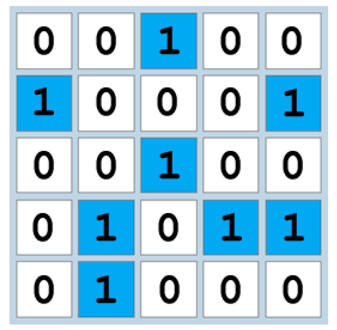
- Configuration—i.e., allocation of filled cells in the grid, coded as a matrix of 1s (corresponding to the cells filled with blue) and 0s (corresponding to the blank cells)—see example in Figure 5.
From the above, several derived independent variables were obtained. To apply the compression algorithms, we converted each configuration into bit strings using two ways: by rows (an example matrix [[1,1],[0,0]] becomes [1100] string) and by columns (the same matrix becomes [1010]), in both cases starting from the top left element.
- Length of the shortest string compressed with the RLE algorithm (from the row-based or the column-based conversion): LRLE;
- Length of the shortest string compressed with the RLE algorithm (from the row-based or the column-based conversion): LDEF;
- Number of figures composed from adjacent cells based on the range 1 von Neumann neighborhood rule (elements that touch diagonally do not constitute a figure): FN;
- Number of figures composed from adjacent cells based on the range 1 Moore neighborhood rule (elements that touch diagonally do constitute a figure): FM.
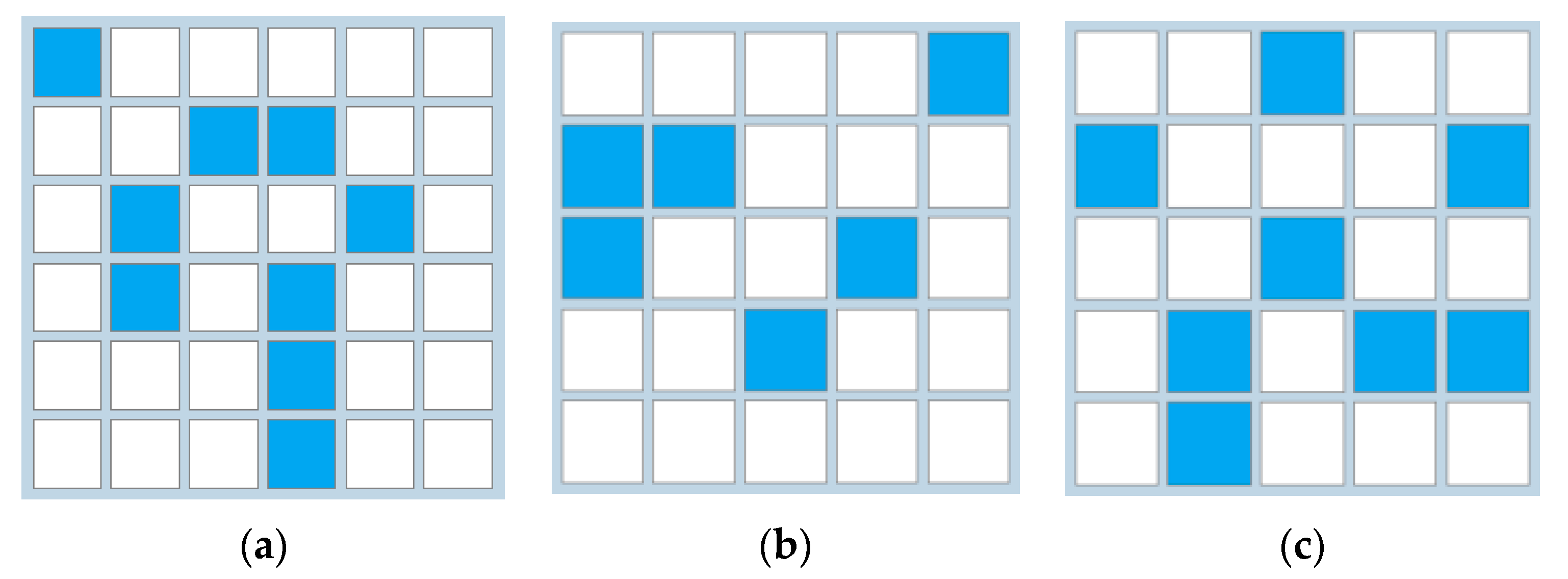
In Figure 6 we present some example configurations, for which the corresponding values are the following: (a) FN = 5, FM = 2; (b) FN = 4, FM = 3; (c) FN = 6, FM = 4.
The dependent variables were:
- the number of correctly designated cells in a trial (SC);
- the performance time in the trial (TM)—excluding the 2 s of the initial blue cells demonstration;
- the subjective evaluation of the configuration’s visual complexity, for which we used 5-point Likert scale (1 being “low complexity” and 5 being “high complexity”): Complexity.
One more dependent variable was a derived one—for each trial, we would calculate the error level (EM):
3.4. Subjects
In the first round of our experiment, there were 88 participants (26 males, 62 females). They were Bachelor and Master students of Novosibirsk State Technical University (NSTU), who took part in the experiment voluntary (no random selection was performed). Their age ranged from 16 to 22, mean 19.4 (SD = 1.1). All the participants had normal or corrected to normal vision and reasonable experience in using computers and mouse. They employed desktop computer equipment and software installed in the university computer rooms, all having similar parameters, particularly monitor sizes and screen resolutions. The approval for the study with humans was provided by Novosibirsk State Technical University, based on the internal regulations.
The number of valid subjects in the second round of the experiment was 78 (57 females, 20 males, 1 undefined). Most of them were also Bachelor and Master students of NSTU, who took part in the experiment voluntary (no random selection was performed), and only 2 of them (2.6%) had also participated in the first round. The subjects’ age ranged from 17 to 65, mean 21.7 (SD = 2.03). All the participants had normal or corrected to normal vision and reasonable experience in IT usage. Most of the participants worked from desktop computers installed in the university computer rooms. There were also 17 other registrations with the online surveying system, but none of those subjects completed the assignment (on average, each of them completed only 4.4% of the assigned evaluations), so they were discarded from the experiment.
4. Results
The dataset with the experimental data is available from the authors upon request. The analysis was performed with SPSS statistical software.
4.1. Descriptive Statistics
In the first round of the experiment, data for 5243 trials were collected, of which 4607 (87.9%) were considered valid. We excluded mistakes and outliers: outcomes for which the performance time exceeded the working memory limit (TM > 14 s), when subjects did not actually perform the task (TM ≤ 0 s), or when the error level was too high (EM > 0.75), implying negligence by the subject. In the second round of the experiment, the participants submitted in total 7800 complexity evaluations, which were averaged for each configuration. Of the configurations that resulted from the first round, 4546 (98.7%) received enough valid evaluations to be used in further analysis. In Table 1 we show ranges, means, and standard deviations (SD) for the independent and dependent variables.
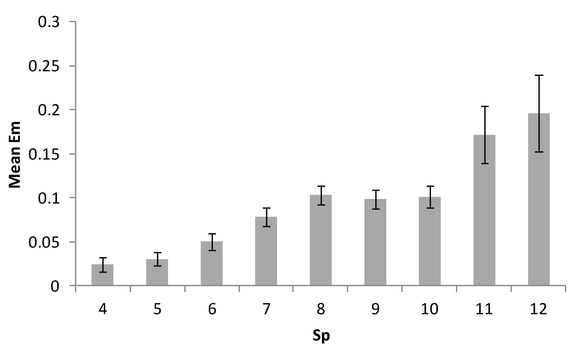
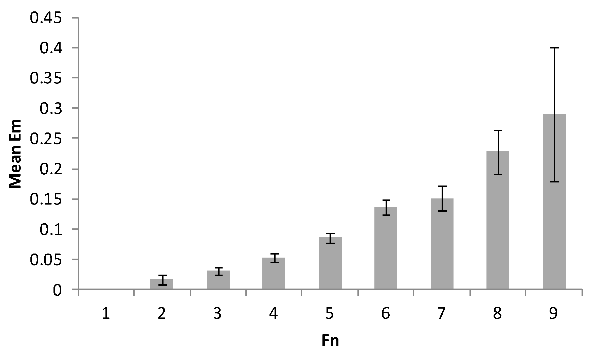
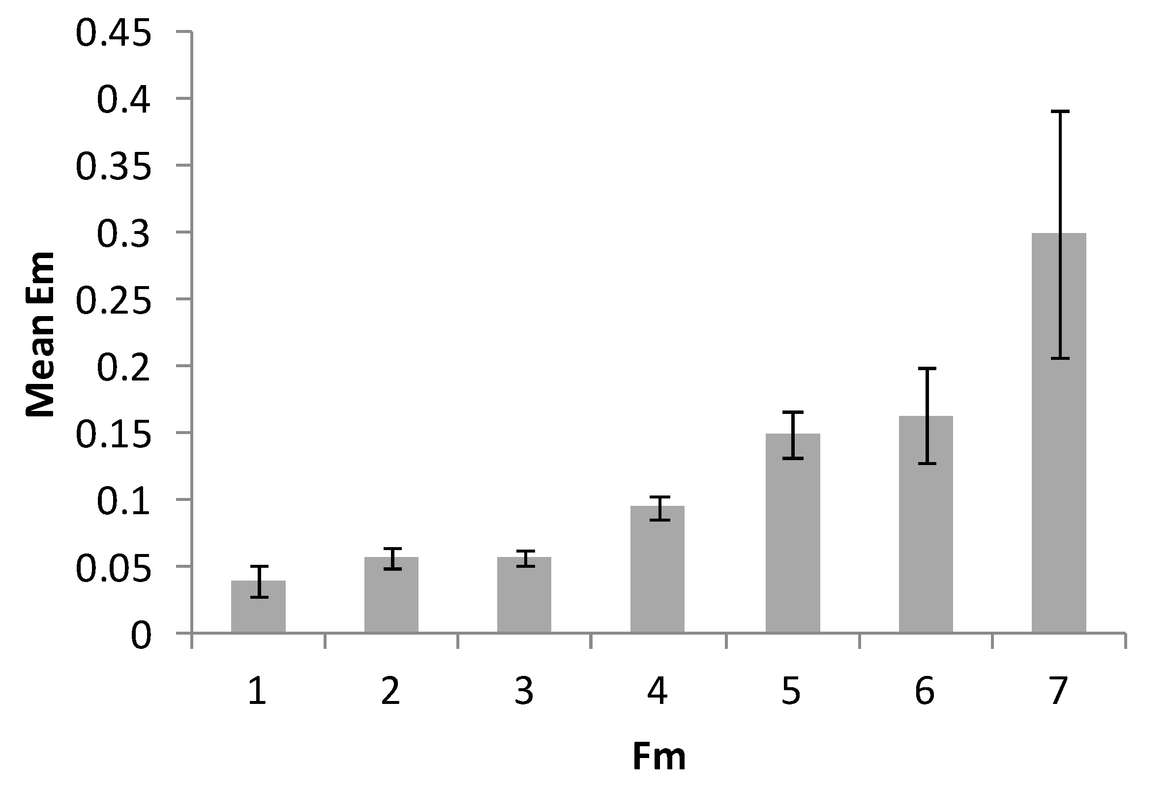
In Figure 7, Figure 8 and Figure 9 we present the diagrams that show mean values for EM due to the independent variables corresponding to the three possible ways to define the memorized information items (NI): SP, FN, and FM, respectively. The mean errors for the rightmost values are not presented, since the amounts of trials for the maximum number of filled cells and figures were too low. From the diagrams, one can note that for FN, the error shows a sharp increase in the range corresponding to Miller’s 7 ± 2 number, whereas for SP no such effect can be observed. For FM, no conclusion could be made due to its limited range.
4.2. Correlation Analysis
The Pearson correlation between EM and TM was positive and significant (r4546 = 0.14; p < 0.001), which was to be expected, since more difficult tasks were both prone to errors and required more time to complete. It may also imply that extra time spent in the task did decrease the chances to extract the elements’ correct positions from working memory, which could start to decay. The positive correlation (non-parametric Kendall Tau-b for ordinal scales) between Complexity and TM (τ4546 = 0.218; p < 0.001) was somehow stronger than between Complexity and EM (τ4546 = 0.196; p < 0.001).
The correlations between the independent and the main dependent variables are presented in Table 2, all correlations are significant (p < 0.001). One can note that the strongest correlate for EM was FN, while for Complexity it was SP (highlighted in bold), which suggest support for Hypothesis 2 rather than Hypothesis 1. The strongest correlate for TM was SP (r4546 = 0.408, p < 0.001), which seems obvious, since the subjects had to designate each memorized cell by clicking it.
4.3. Regression Analysis
To construct regression model for EM, we used backwards variable selection method with the 6 independent variables (listed in the Table 1 above) plus log2SP that represented Hick’s law. In the resulting model, 4 factors were significant: FN (Beta = 0.203, p < 0.001), SP (Beta = 0.143, p < 0.001), FM (Beta = 0.104, p < 0.001), S0 (Beta = 0.052, p = 0.001). However, R2 = 0.134 of the model was rather low (F4,4541 = 176.1, p < 0.001):
In a similar fashion, we constructed regression model for Complexity, in which the backwards variable selection method yielded 4 significant factors out of the 7 candidate ones: log2SP (Beta = 0.345, p < 0.001), FN (Beta = 0.182, p < 0.001), LRLE (Beta = 0.122, p < 0.001), LDEF (Beta = 0.039, p = 0.037). The model had somehow improved R2 = 0.342 (F4,4541 = 590.4, p < 0.001):
As expected, the best predictors for Complexity were the ones based on information theory and compression, with the exception of FN. On the contrary, the model for accuracy in VSWM tasks included no such predictors, which reinforces Hypothesis 2 and refutes Hypothesis 1. In the next sub-chapter, we address Hypothesis 3 related to the index of difficulty.
4.4. Index of Difficulty
In our formulation for the index of difficulty in accordance with (11), we considered three possible options for the memorized information items NI = {SP, FN, FM}, corresponding to the significant factors we previously found in (13):
In Table 3 we present the candidate indexes’ ranges, means, SDs and correlations (all of them significant, p < 0.001) with the dependent variables. As expected, due to the designation stage, TM had the highest correlation (r4546 = 0.390) with IDMSP, which was also the strongest correlate for Complexity (r4546 = 0.421). However, for EM, the highest correlation (r4546 = 0.340) was found with IDMFN, which was even higher than with FN (see in Table 2 above), which supports Hypothesis 3.
In the regression analysis for EM, we first calculated its average values per levels of each of the index of difficulty formulations (unlike in Fitts’ law, we don’t do it per trials, since we predict not time, but accuracy), as well as per each level of Complexity. We obtained the following regression equations with the respective statistics:
R2 = 0.597, F1,15 = 22.2, p < 0.001
R2 = 0.893, F1,16 = 133.5, p < 0.001
R2 = 0.827, F1,13 = 62.2, p < 0.001
R2 = 0.572, F1,20 = 26.7, p < 0.001
The model (21) with Complexity had the lowest R2, while the model with IDMFN (19) explained the most variation in EM, and we will be using this formulation in further analysis. The regression model for performance time due to this factor had R2 = 0.474 (F1,16 = 14.4, p = 0.002):
The lower degree of variation explained by the index of difficulty in TM compared to EM is natural, since the former is affected not only by the working memory capabilities, but also by skill with a computer mouse that was used in the designation stage in the experiment.
4.5. Effective Index of Difficulty and VSWM Throughput
Proper formulation of throughput—one that accounts for both speed and accuracy of the task performance—needs to be based on the difficulty of the task “effectively” performed by the subject. In our IDM formulation (11), “effective” NI would correspond to the information items correctly memorized and designated (clicked), which we can obtain by multiplying the nominal number of the information items by the accuracy level. Effective S0, the area that is actually searched through by the subject, should depend of the placement of the items. For the purpose of the current study, we assume that the subject always searched the whole area and thus, in a way, use the nominal S0. Thus, the formulation for the effective index of difficulty for VSWM tasks is:
Thus, calculated effective IDMeFN in our experiment ranged from 3.45 to 46.53 bit, mean = 20.47 (SD = 6.71). Its correlation with the nominal IDMFN was significant: r4546 = 0.831, p < 0.001. However, the effective index of difficulty had weaker correlation r4546 = −0.218 (p < 0.001) with EM than the nominal IDMFN (r4546 = 0.340, see in Table 3 above), so instead of replacing the latter with the effective one, let us introduce the effective time.
Given the relation between the nominal and the effective indexes of difficulty, we can re-write the throughput equation (6) as follows:
where TMe is effective time, which basically involves penalty for error-making.
The mean value for the effective time in our experiment was 6.88 s (SD = 3.35). The correlation between TMe and IDMFN was r4546 = 0.297 (p < 0.001), which is higher than r4546 = 0.211 that we previously found between the nominal TM and IDMFN (see in Table 3 above). The regression model for TMe and IDMFN, which can be seen as an equivalent to Fitts’ law, was highly significant (F1,16 = 150.0, p < 0.001) and had R2 = 0.904, i.e., higher than both for TM in (22) and for EM in (19):
The TPM calculated for our experiment data (averaged for all the valid trials) was 3.75 bit/s (SD = 1.69). Its correlation with Complexity was not significant (τ4546 = 0.011, p = 0.314), so TPM can be recognized as a measure independent of a particular task setup in a given experiment. ANOVA showed that TPM averaged per participants was significantly different due to subject’s gender (F1,86 = 3.87, p = 0.05, η2 = 0.0435), the mean values being 3.9 bit/s for males and 3.6 bit/s for females. The effect of gender on error was not significant (F1,86 = 2.91; p = 0.09). All in all, absolute values of TPM in our experiment suggest strong support for Hypothesis 4, as we discuss further on.
5. Discussion
Automation of design and validation of user interfaces for human–computer systems is essential for the development of the internet ecosystem, adoption of smart systems, etc. Effective organization of the interaction necessitates that human needs and limitations, particularly in the cognitive aspects, are expressed quantitatively and are properly accounted for [48]. In our work, we explored different predictors that characterize the difficulty of tasks engaging visual-spatial working memory, which are relatively rarely covered in the currently existing computational models of user behavior, unlike e.g., visual attention [25] or visual complexity [49].
The results of our analysis suggest that Hypothesis 1 has to be rejected in favor of Hypothesis 2, as the compression-based metrics of visual complexity (LRLE, LDEF), as well as Hick’s law information theoretic metric, were inferior to the proximity-based metrics, as demonstrated by the regression equation for EM (13). The compression-based factors and the Hick’s law factor were significant in the regression equation for Complexity (14), which replicated our previous findings [12], even though in that work, we did not test FN and FM as the candidate factors for VC. That said, the actual subjective evaluations of VC did have significant positive correlation to the measures of performance in VSWM-related tasks: τ4546 = 0.196 (p < 0.001) for EM and τ4546 = 0.218 (p < 0.001) for TM. The practicality of collecting the subjective evaluations from users is doubtful though, as the performance can be better predicted with the metrics that can be automatically evaluated from the configurations.
Indeed, our study suggests that Hypothesis 3 should be accepted, as the proposed index of difficulty (16) had the highest correlation with the performance in VSWM-related tasks (as operationalized with EM): r4546 = 0.340 (p < 0.001). Of the three candidate factors (NI), the formulation of IDM that uses the number of von Neumann figures (FN) as the memorized item showed clear advantage in correlation (see Table 3) and regression analyses (19). It is also aligned with Hypothesis 2, and FN showed the best match to the 7 ± 2 information chunks limit found by Miller and colleagues for working memory.
Hypothesis 4 should also be accepted, as the value of throughput obtained in our experiment, 3.75 bit/s, is consistent with the ones reported in the literature: 2–4 bit/s for human operator tasks relying on working memory [37,39,40]. The Fitts’ throughput values generally found for computer mouse, which the subjects used in the designation stage of the experiment, are also coherent: 3.7–4.9 bit/s [30]. The significant effect of gender on time that we found, 3.9 bit/s for males and 3.6 bit/s for females, is in line with the general advantage of younger males in both spatial orientation tasks and motor reaction speed, which is well described in the existing works [50,51]. At the same time, the difference in accuracy between the genders is often non-existent [52], and in our experiment, it was not significant either (p = 0.09).
The limitations of our research, first of all, include relatively low values for correlations and R2 coefficients in the regression analysis for the per-trial data. Indeed, many established user behavior models have higher R2 values, particularly Fitts’ law, for which R2s of over 0.9 are generally reported [30]. On the other hand, for models involving Hick’s law, the fit is generally lower, e.g., in [34], they reported R2 = 0.52 for traditional menu selection. The discrepancy in our study is explained in part by the experimental procedure, which included not only memorization, but also motor behavior-based designation stage, i.e., clicking the memorized cells. Because of the fusion of the two task types, the number of uncontrolled factors amplified, particularly since we did not consider the difficulty of the movement tasks. Indeed, the absolute R2 values could have been increased by including more variables in the regression equation, since the potential number of perceived regularities is unlimited, but our main goal was comparison of the factors’ effects, not accurate models. At the same time, regression analysis for the data averaged per IDMFN values (so that the bias factors were negated) yielded rather high values of R2 about 0.9, for both EM (19) and TeM (25).
Biases to conceptual validity of our study include the formulation of IDM (11), which is novel to the field and should require further verification. Particularly, its units of measurement are not the same bits as the ones in Fitts’ law or the information-theoretic bits, so that they should probably be called “spatial bits”, as they result from multiplication of the information and spatial components of the complexity. This assumption seems justified on neurophysiologic level, since information processing in VSWM is carried out in two distinct streams of the brain (ventral and dorsal) but needs further investigation. Also, visual complexity was measured in a survey, so a subjectivity bias might have been introduced. However, this is a widely used method for quantification of VC, which is rather inexorable since the subjects performed no interactions with the grids in the experiment (due to the very nature of visual complexity), so that their responses to the stimuli were scarce.
External validity of our study is somehow limited by the low diversity of participants engaged in our experiments: they were all young and skilled with computers. That said, we need to highlight that we did not seek to develop generalizable user behavior models, but to compare the effects of factors. Still, in the future, we plan to explore the subjects of various demographics to see if the found effects preserve, and if not, what it can tell about the variability of cognitive processes and complexity perception. For instance, it was previously found that elder people sometimes can reproduce information from working memory even quicker that younger ones due to its decreased capacity associated with inhibition processes [53].
Our future research directions also include further detailing of the proposed IDM formulation. Particularly, we plan to introduce the log2k multiplier to its informational component, in accordance with Hartley’s formula for the quantity of information (a fixed k = 2 was used in the current study, corresponding to a blank or a filled cell). For detailing the spatial component, we intend to look into the spatial entropy and cell automata complexity measures.
6. Conclusions
We see the main contributions of our study in factors affecting the performance in VSWM-related tasks as follows:
- We demonstrated that the information-theoretic and compression algorithms-based metrics that are known to be representative of visual complexity do not adequately predict performance in tasks that engage visual-spatial working memory.
- We found that the memorized information chunks in 2D area containing uniform cells are not individual elements, but figures composed per the range 1 von Neumann neighborhood rule.
- We proposed the corresponding formulation for the index of difficulty for the tasks engaging visual-spatial working memory (16), quantitatively expressing it in “spatial bits”.
- We outlined the approach for calculating throughput (24), which can be used to predict users’ memorization performance with different designs of a GUI screen. We also believe that the approach can be generalized to other tasks that emerge in HCI.
We believe that the results of our study can be of practical usage in UI design and development. In a manner similar to Fitts’ law application for optimizing movements and pointing [30], IDM can be used to refine the layout of UI elements in order to lower VSWM load. Several candidate UI designs can be compared with respect to the achieved user performance using the TPM measure. The discovered stronger influence of Gestalt principles-based factors suggests that these approaches might be preferred over the currently utilized compression-based visual complexity measures, although this requires further practical exploration.
7. Patents
“Software for measuring complexity and performance in tasks engaging visual-spatial working memory” (M. Bakaev, R. Petrov, O. Razumnikova, V. Khvorostov), No. 2018610926, awarded by the Russian Federal Service for Intellectual Property (2018).
Author Contributions
Conceptualization, M.B.; methodology, M.B. and O.R.; software, M.B.; validation, M.B.; formal analysis, M.B.; investigation, M.B.; resources, M.B. and O.R.; data curation, M.B. and O.R.; writing—original draft preparation, M.B.; writing—review and editing, O.R.; visualization, M.B.; funding acquisition, O.R. All authors have read and agreed to the published version of the manuscript.
Funding
The reported study was funded by RFBR according to the research project No. 19-29-01017.
Institutional Review Board Statement
The study was conducted according to the guidelines of the Declaration of Helsinki, and approved by the Institutional Review Board of Novosibirsk State Technical University, #11 of 23 Nov 2016.
Informed Consent Statement
Informed consent was obtained from all subjects involved in the study.
Data Availability Statement
The data presented in this study are available on request from the corresponding author. The data are not publicly available due to privacy considerations.
Acknowledgments
We thank Vladimir Khvorostov and Roman Petrov who provided technical assistance in development and using the software for the data collection.
Conflicts of Interest
The authors declare no conflict of interest.
Appendix A
The encode function implements simple RLE algorithm compression. The input variable for the function is binary string.
function encode($input)
{
if (!$input) {
return “;
}
$output = “;
$prev = $letter = null;
$count = 1;
foreach (str_split($input) as $letter) {
if ($letter === $prev) {
$count++;
} else {
if ($count > 1) {
$output .= $count;
}
$output .= $prev;
$count = 1;
}
$prev = $letter;
}
if ($count > 1) {
$output .= $count;
}
$output .= $letter;
return $output;
}
References
- Oulasvirta, A. Can computers design interaction? In Proceedings of the 8th ACM SIGCHI Symposium on Engineering Interactive Computing Systems, Brussels, Belgium, 21–24 June 2016; pp. 1–2. [Google Scholar]
- Bailly, G.; Oulasvirta, A.; Brumby, D.P.; Howes, A. Model of visual search and selection time in linear menus. Proc. SIGCHI Conf. Hum. Factors Comput. Syst. 2014, 3865–3874. [Google Scholar] [CrossRef] [Green Version]
- Chen, X.; Starke, S.D.; Baber, C.; Howes, A. A cognitive model of how people make decisions through interaction with visual displays. In Proceedings of the 2017 CHI Conference on Human Factors in Computing Systems, Denver, CO, USA, 6–11 May 2017; pp. 1205–1216. [Google Scholar]
- Chen, X.; Bailly, G.; Brumby, D.P.; Oulasvirta, A.; Howes, A. The emergence of interactive behavior: A model of rational menu search. In Proceedings of the 33rd Annual ACM Conference on Human Factors in Computing Systems, Seoul, Korea, 18–23 April 2015; pp. 4217–4226. [Google Scholar]
- Tseng, Y.-C.; Howes, A. The adaptation of visual search to utility, ecology and design. Int. J. Hum. Comput. Stud. 2015, 80, 45–55. [Google Scholar] [CrossRef] [Green Version]
- Gray, W.D.; Sims, C.R.; Fu, W.-T.; Schoelles, M.J. The soft constraints hypothesis: A rational analysis approach to resource allocation for interactive behavior. Psychol. Rev. 2006, 113, 461–482. [Google Scholar] [CrossRef] [PubMed] [Green Version]
- Miniukovich, A.; Marchese, M. Relationship between Visual Complexity and Aesthetics of Webpages. In Proceedings of the 2020 CHI Conference on Human Factors in Computing Systems, Honolulu, HI, USA, 25–30 April 2020; pp. 1–13. [Google Scholar]
- Rosenholtz, R.; Li, Y.; Nakano, L. Measuring visual clutter. J. Vis. 2007, 7, 17–22. [Google Scholar] [CrossRef] [PubMed] [Green Version]
- Carballal, A.; Santos, A.; Romero, J.; Machado, J.T.A.P.; Correia, J.; Castro, L. Distinguishing paintings from photographs by complexity estimates. Neural Comput. Appl. 2018, 30, 1957–1969. [Google Scholar] [CrossRef]
- Chang, L.-Y.; Chen, Y.-C.; Perfetti, C.A. GraphCom: A multidimensional measure of graphic complexity applied to 131 written languages. Behav. Res. Methods 2017, 50, 427–449. [Google Scholar] [CrossRef] [Green Version]
- Reinecke, K.; Yeh, T.; Miratrix, L.; Mardiko, R.; Zhao, Y.; Liu, J.; Gajos, K.Z. Predicting users’ first impressions of website aesthetics with a quantification of perceived visual complexity and colorfulness. In Proceedings of the SIGCHI Conference on Human Factors in Computing Systems, Paris, France, 27 April–2 May 2013; pp. 2049–2058. [Google Scholar]
- Bakaev, M.; Goltsova, E.; Khvorostov, V.; Razumnikova, O. Data Compression Algorithms in Analysis of UI Layouts Visual Complexity. In International Andrei Ershov Memorial Conference on Perspectives of System Informatics; Springer: Cham, Switzerland, 2019; pp. 167–184. [Google Scholar]
- Harper, S.; Michailidou, E.; Stevens, R. Toward a definition of visual complexity as an implicit measure of cognitive load. ACM Trans. Appl. Percept. TAP 2009, 6, 1–18. [Google Scholar] [CrossRef]
- Schnur, S.; Bektaş, K.; Çöltekin, A. Measured and perceived visual complexity: A comparative study among three online map providers. Cartogr. Geogr. Inf. Sci. 2018, 45, 238–254. [Google Scholar] [CrossRef]
- Kondyli, V.; Bhatt, M.; Suchan, J. Towards a Human-Centred Cognitive Model of Visuospatial Complexity in Everyday Driving. arXiv 2020, arXiv:2006.00059. [Google Scholar]
- Conway, A.R.; Cowan, N.; Bunting, M.F.; Therriault, D.J.; Minkoff, S.R. A latent variable analysis of working memory capacity, short-term memory capacity, processing speed, and general fluid intelligence. Intelligence 2002, 30, 163–183. [Google Scholar] [CrossRef]
- Unsworth, N.; Fukuda, K.; Awh, E.; Vogel, E.K. Working Memory Delay Activity Predicts Individual Differences in Cognitive Abilities. J. Cogn. Neurosci. 2015, 27, 853–865. [Google Scholar] [CrossRef] [PubMed] [Green Version]
- Cowan, N. Chapter 20 What are the differences between long-term, short-term, and working memory? Prog. Brain Res. 2008, 169, 323–338. [Google Scholar] [CrossRef] [PubMed] [Green Version]
- Aben, B.; Stapert, S.Z.; Blokland, A. About the Distinction between Working Memory and Short-Term Memory. Front. Psychol. 2012, 3, 301. [Google Scholar] [CrossRef] [PubMed] [Green Version]
- Cowan, N. The magical mystery four: How is working memory capacity limited, and why? Curr. Dir. Psychol. Sci. 2010, 19, 51–57. [Google Scholar] [CrossRef] [PubMed] [Green Version]
- Cowan, N. Working memory maturation: Can we get at the essence of cognitive growth? Perspect. Psychol. Sci. 2016, 11, 239–264. [Google Scholar] [CrossRef] [PubMed]
- Emacken, B.; Etaylor, J.; Ejones, D. Limitless capacity: A dynamic object-oriented approach to short-term memory. Front. Psychol. 2015, 6, 293. [Google Scholar] [CrossRef] [Green Version]
- Proctor, R.W.; Schneider, D.W. Hick’s Law for Choice Reaction Time: A Review. Q. J. Exp. Psychol. 2017, 24, 1–56. [Google Scholar] [CrossRef]
- Baddeley, A.D.; Logie, R.H. Working memory: The multiple-component model. In Models of Working Memory: Mechanisms of Active Maintenance and Executive Control; Miyake, A., Shah, P., Eds.; Cambridge University Press: Cambridge, UK, 1999; pp. 28–61. [Google Scholar]
- Filipe, S.; Alexandre, L.A. From the human visual system to the computational models of visual attention: A survey. Artif. Intell. Rev. 2013, 39, 1–47. [Google Scholar]
- Peterson, D.J.P.; Berryhill, M.E. The Gestalt principle of similarity benefits visual working memory. Psychon. Bull. Rev. 2013, 20, 1282–1289. [Google Scholar] [CrossRef] [Green Version]
- Gao, Z.; Gao, Q.; Tang, N.; Shui, R.; Shen, M. Organization principles in visual working memory: Evidence from sequential stimulus display. Cognition 2016, 146, 277–288. [Google Scholar] [CrossRef]
- Kałamała, P.; Sadowska, A.; Ordziniak, W.; Chuderski, A. Gestalt Effects in Visual Working Memory. Exp. Psychol. 2017, 64, 5–13. [Google Scholar] [CrossRef] [PubMed] [Green Version]
- Schneider, D.W.; Anderson, J.R. A memory-based model of Hick’s law. Cogn. Psychol. 2011, 62, 193–222. [Google Scholar] [CrossRef] [PubMed] [Green Version]
- Soukoreff, R.W.; MacKenzie, I.S. Towards a standard for pointing device evaluation, perspectives on 27 years of Fitts’ law research in HCI. Int. J. Hum. Comput. Stud. 2004, 61, 751–789. [Google Scholar] [CrossRef]
- Seow, S. Information Theoretic Models of HCI: A Comparison of the Hick-Hyman Law and Fitts’ Law. Hum. Comput. Interact. 2005, 20, 315–352. [Google Scholar] [CrossRef]
- Landauer, T.K.; Nachbar, D.W. Selection from alphabetic and numeric menu trees using a touch screen: Breadth, depth, and width. In Proceedings of the CHI ‘85 Conference: Human Factors in Computer Systems, San Francisco, CA, USA, 14–18 April 1985; pp. 73–78. [Google Scholar]
- Bakaev, M.; Avdeenko, T.; Cheng, H.-I. Modelling selection tasks and assessing performance in web interaction. IADIS Int. J. Comput. Sci. Inf. Syst. 2012, 7, 94–105. [Google Scholar]
- Cockburn, A.; Gutwin, C.; Greenberg, S. A predictive model of menu performance. In Proceedings of the SIGCHI Conference on Human Factors in Computing Systems, San Jose, CA, USA, 27 April–2 May 2007; pp. 627–636. [Google Scholar]
- Longstreth, L.E.; El-Zahhar, N.; Alcorn, M.B. Exceptions to Hick’s law: Explorations with a response duration measure. J. Exp. Psychol. Gen. 1985, 114, 417–434. [Google Scholar] [CrossRef]
- Huesmann, L.R.; Card, S.K.; Moran, T.P.; Newell, A. The Psychology of Human-Computer Interaction. Am. J. Psychol. 1984, 97, 625. [Google Scholar] [CrossRef]
- Prisnyakov, V.F.; Prisnyakova, L.M. Mathematic Modeling of Information Processing by Human-Machine Systems’ Operator; Mashinostroenie: Moscow, Russia, 1990. (In Russian) [Google Scholar]
- Bakaev, M.; Avdeenko, T. A quantitative measure for information transfer in human-machine control systems. In Proceedings of the 2015 International Siberian Conference on Control and Communications (SIBCON), Omsk, Russia, 21–23 May 2015; pp. 1–4. [Google Scholar]
- Pierce, B.F.; Woodson, W.E.; Conover, D.W. Human Engineering Guide for Equipment Designers. Technol. Cult. 1966, 7, 124. [Google Scholar] [CrossRef]
- Sperling, G. A Model for Visual Memory Tasks. Hum. Factors J. Hum. Factors Ergon. Soc. 1963, 5, 19–31. [Google Scholar] [CrossRef]
- Solomonoff, R. The application of algorithmic probability to problems in artificial intelligence. Mach. Intell. Pattern Recognit. 1986, 4, 473–491. [Google Scholar]
- Wagemans, J.; Elder, J.H.; Kubovy, M.; Palmer, S.E.; Peterson, M.A.; Singh, M.; von der Heydt, R. A century of Gestalt psychology in visual perception: I. Perceptual grouping and figure–ground organization. Psychol. Bull. 2012, 138, 1172–1217. [Google Scholar] [CrossRef] [PubMed] [Green Version]
- Donderi, D.C. Visual complexity: A review. Psychol. Bull. 2006, 132, 73. [Google Scholar] [CrossRef] [PubMed] [Green Version]
- Robinson, A.; Cherry, C. Results of a prototype television bandwidth compression scheme. Proc. IEEE 1967, 55, 356–364. [Google Scholar] [CrossRef]
- Deutsch, P. DEFLATE Compressed Data Format Specification Version 1.3. 1996. Available online: https://0-dl-acm-org.brum.beds.ac.uk/doi/pdf/10.17487/RFC1951 (accessed on 18 January 2021).
- Bakaev, M.A.; Razumnikova, O. Defining complexity for visual-spatial memory tasks and human operator s throughput. Upr. Bol’shimi Sist. 2017, 70, 25–57. (In Russian) [Google Scholar]
- Wolfe, J.M. Saved by a log: How do humans perform hybrid visual and memory search? Psychol. Sci. 2012, 23, 698–703. [Google Scholar] [CrossRef]
- Xing, J. Measures of Information Complexity and the Implications for Automation Design; No. DOT/FAA/AM-04/17; Federal Aviation Administration: Washington, DC, USA; Oklahoma City Ok Civil Aeromedical Inst.: Oklahoma City, OK, USA, 2004. [Google Scholar]
- Miniukovich, A.; Sulpizio, S.; De Angeli, A. Visual complexity of graphical user interfaces. In Proceedings of the 2018 International Conference on Big Data and Education, Honolulu, HI, USA, 9–11 March 2018; p. 20. [Google Scholar]
- Blough, P.M.; Slavin, L.K. Reaction time assessments of gender differences in visual-spatial performance. Percept. Psychophys. 1987, 41, 276–281. [Google Scholar] [CrossRef] [Green Version]
- Halpern, D.F. Sex Differences in Cognitive Abilities, 3rd ed.; Psychology Press: New York, NY, USA, 2013. [Google Scholar]
- Loring-Meier, S.; Halpern, D.F. Sex differences in visuospatial working memory: Components of cognitive processing. Psychon. Bull. Rev. 1999, 6, 464–471. [Google Scholar] [CrossRef]
- Razumnikova, O.M.; Volf, N.V. Re-organization of relation of intelligence with attention and memory in aging. Zhurnal Vyss. Nervn. Deyatelnosti Im. I.P. Pavlov. 2017, 67, 55–67. (In Russian) [Google Scholar]
Figure 1.
Outline of the Human Processor model.

Figure 2.
Illustrations of von Neumann (a) and Moore (b) neighborhoods of range 1.

Figure 3.
An example stimuli configuration with 3 squares that compose 3 von Neumann figures or 1 Moore figure (a screenshot from the software that we used in the experiment).
Figure 3.
An example stimuli configuration with 3 squares that compose 3 von Neumann figures or 1 Moore figure (a screenshot from the software that we used in the experiment).

Figure 4.
An example of a completed trial: the designation was performed incorrectly, and the correct location of the squares is shown to the participant (a screenshot from the software that we used in the experiment).
Figure 4.
An example of a completed trial: the designation was performed incorrectly, and the correct location of the squares is shown to the participant (a screenshot from the software that we used in the experiment).

Figure 5.
Example of the grid configuration with the numerical values corresponding to the cells.

Figure 6.
Examples of the grid configuration with the numerical values corresponding to the cells.

Figure 7.
Mean error level per the number of information items, filled cells (SP).

Figure 8.
Mean error level per the number of information items, von Neumann neighborhood (FN).

Figure 9.
Mean error level per the number of information items, Moore neighborhood (FM).


Table 1.
Descriptive statistics for the variables in the experiment.
| Variable | Range | Mean (SD) |
|---|---|---|
| S0 | 25, 36 | - |
| SP | 4–13 | 7.42 (1.99) |
| FN | 1–10 | 4.58 (1.42) |
| FM | 1–8 | 3.21 (1.19) |
| LRLE | 8–30 | 17.07 (3.52) |
| LDEF | 8–20 | 13.91 (1.98) |
| SC | 1–13 | 6.76 (1.96) |
| EM | 0–0.75 | 0.08 (0.14) |
| TM | 1–14 s | 6.03 (2.21) |
| Complexity | 1.0–5.0 | 2.57 (0.96) |
Table 2.
Correlations of the independent variables with EM (Pearson) and Complexity (Kendall tau-b).
Table 2.
Correlations of the independent variables with EM (Pearson) and Complexity (Kendall tau-b).
| Variable | r (EM) | τ (Complexity) |
|---|---|---|
| S0 | 0.176 | 0.13 |
| SP | 0.231 | 0.424 |
| FN | 0.332 | 0.329 |
| FM | 0.239 | 0.115 |
| LRLE | 0.302 | 0.410 |
| LDEF | 0.215 | 0.342 |
Table 3.
Descriptive statistics and correlations for the different formulations of the index of difficulty.
Table 3.
Descriptive statistics and correlations for the different formulations of the index of difficulty.
| Index of Difficulty | Range | Mean (SD) | r (EM) | r (TM) | τ (Complexity) |
|---|---|---|---|---|---|
| IDMSP | 18.6–67.2 | 36.5 (10.2) | 0.259 | 0.390 | 0.421 |
| IDMFN | 4.6–51.7 | 22.6 (7.5) | 0.340 | 0.211 | 0.314 |
| IDMFM | 4.6–41.4 | 15.9 (6.3) | 0.251 | 0.068 | 0.124 |
Publisher’s Note: MDPI stays neutral with regard to jurisdictional claims in published maps and institutional affiliations. |
© 2021 by the authors. Licensee MDPI, Basel, Switzerland. This article is an open access article distributed under the terms and conditions of the Creative Commons Attribution (CC BY) license (http://creativecommons.org/licenses/by/4.0/).
Share and Cite
MDPI and ACS Style
Bakaev, M.; Razumnikova, O. What Makes a UI Simple? Difficulty and Complexity in Tasks Engaging Visual-Spatial Working Memory. Future Internet 2021, 13, 21. https://0-doi-org.brum.beds.ac.uk/10.3390/fi13010021
AMA Style
Bakaev M, Razumnikova O. What Makes a UI Simple? Difficulty and Complexity in Tasks Engaging Visual-Spatial Working Memory. Future Internet. 2021; 13(1):21. https://0-doi-org.brum.beds.ac.uk/10.3390/fi13010021
Chicago/Turabian StyleBakaev, Maxim, and Olga Razumnikova. 2021. "What Makes a UI Simple? Difficulty and Complexity in Tasks Engaging Visual-Spatial Working Memory" Future Internet 13, no. 1: 21. https://0-doi-org.brum.beds.ac.uk/10.3390/fi13010021
Note that from the first issue of 2016, this journal uses article numbers instead of page numbers. See further details here.