Article

Architecture for Enabling Edge Inference via Model Transfer from Cloud Domain in a Kubernetes Environment

VTT Technical Research Centre of Finland, 90571 Oulu, Finland
*
Author to whom correspondence should be addressed.
Submission received: 20 November 2020 / Revised: 23 December 2020 / Accepted: 24 December 2020 / Published: 29 December 2020
(This article belongs to the Section Network Virtualization and Edge/Fog Computing)

Abstract

:
The current approaches for energy consumption optimisation in buildings are mainly reactive or focus on scheduling of daily/weekly operation modes in heating. Machine Learning (ML)-based advanced control methods have been demonstrated to improve energy efficiency when compared to these traditional methods. However, placing of ML-based models close to the buildings is not straightforward. Firstly, edge-devices typically have lower capabilities in terms of processing power, memory, and storage, which may limit execution of ML-based inference at the edge. Secondly, associated building information should be kept private. Thirdly, network access may be limited for serving a large number of edge devices. The contribution of this paper is an architecture, which enables training of ML-based models for energy consumption prediction in private cloud domain, and transfer of the models to edge nodes for prediction in Kubernetes environment. Additionally, predictors at the edge nodes can be automatically updated without interrupting operation. Performance results with sensor-based devices (Raspberry Pi 4 and Jetson Nano) indicated that a satisfactory prediction latency (~7–9 s) can be achieved within the research context. However, model switching led to an increase in prediction latency (~9–13 s). Partial evaluation of a Reference Architecture for edge computing systems, which was used as a starting point for architecture design, may be considered as an additional contribution of the paper.

1. Introduction

Buildings have an important dual role in reducing Green House Gas (GHG) emissions. Firstly, buildings are major consumers of energy (e.g., roughly 40% of the total energy consumption in the EU and U.S. [1,2] comes from buildings). Therefore, even small improvements in energy efficiency are significant if the improvements can be implemented in scalable and cost-efficient way. Secondly, buildings are important to successfully integrate a large share of intermittent generation from renewables such as windmills and solar panels. This is because a significant portion of a building’s energy consumption comes from heating, ventilation, and air conditioning (HVAC) systems [3], and buildings possess a large thermal mass that could be used for demand-side flexibility.
Buildings are not currently operated in the most energy-efficient way, and their thermal capacity is not properly utilised for flexibility management at a global scale. The main technical challenge is that HVAC systems are complex (i.e., consist of chillers, pipes, heat pumps, fans, pumps, boilers, and heat exchangers) and have nonlinear dynamics with long feedback loops caused by thermal inertia of buildings. To address this complex modelling and optimisation challenge, machine learning-based advanced control methods have been proposed in the literature. These approaches can be classified into Reinforcement Learning (RL) and Artificial Neural Network (ANN)-based Model Predictive Control (MPC). The main difference between these approaches is that in RL a control policy is learned directly, whereas in ANN-MPC a model of the system (e.g., a heat demand model) is learned and then used for searching optimal actions. Approaches based both on RL [4,5,6,7] and ANN-MPC [8,9] have been shown to significantly improve energy efficiency when compared to more traditional rule-based control strategies.
Although good results on optimal building energy management have been demonstrated in simulation and small-scale laboratory environments, a lot of work needs to be done in order to replicate the results on a larger scale and in operational environments. In this paper, the goal of energy management is to achieve economic savings for building owners by shifting energy consumption during peak load hours, when the electricity price is high [10]. For realisation of economic savings, energy consumption of buildings must be predicted reliably. Additionally, realisation of automated energy management for buildings is complicated by resource-constraints of edge devices [11], scalability concerns on network bandwidth with a large number of nodes in the edge domain [12], and privacy concerns [12] of building information.
Automation of energy management in buildings is a challenge requiring advanced and continuous on-site data collection (i.e., from building inside temperature and local weather forecasts), prediction, optimisation, and control capabilities for controlling the individual energy loads at buildings. As a technical end-to-end system, an advanced continuous data analytics-based energy management system can be characterised as Information, Communication, Computing and Automation Technology (ICCAT)-based system [13] providing a service of managing energy consumption in individual buildings, where the system has been deployed. Such a system may be realised by placing prediction/inference functionality within a cloud or edge domain (Table 1). In both cases, prediction models may be trained and managed in the cloud domain due to the resource-constraints of edge nodes (e.g., low computing power and memory available). If trained prediction models would be executed (for each building) in the cloud domain, it may create scalability concerns in terms of network bandwidth, when the number of buildings to be managed increases (large number of predictions to be communicated). Constant transfer of predictions may also lead to increased energy consumption at the edge nodes. Additionally, predictions may not be available when the network connection is down between cloud and edge domains (e.g., building in a rural area), and the prediction model is executed in the cloud domain. The downside of placing inference functionality at edge nodes is their lower performance in terms of computing power (CPU/GPU) and memory. Both approaches have privacy concerns regarding the communicated information (prediction model, predictions) between the domains.
While both approaches may be feasible for design and deployment of an energy management system, in this paper model, training and deployment is centralised to the cloud domain while placing inference functionality to the edge domain. The argued benefits of edge inference (vs. cloud inference) is better scalability in terms of the amount of communication needed (constant transfer of predictions is not needed for each building), which may also lead to lower energy consumption at edge nodes (network access is needed less frequently), and independency of operation during a possible network outage. Particularly, a goal is to design and evaluate a distributed computing system architecture, where software-, data- and ML-engineering activities (DevOps [14], ModelOps [15] CI/CD) are centrally supported by cloud computing, but ML-based predictive models are deployed and managed as software for continuous forecasting of building-specific energy consumption at edge computing environments.
Various Reference Architectures (RA) have been designed for edge computing environments for facilitating the design of concrete architectures [16,17]. Also, many choices have been explored for increasing the performance of Machine learning (ML)-based inference in cloud-edge continuum [12]. Further, technologies (e.g., Rancher [18], k3s [19]) have been developed for management of services in cloud and edge computing environments. Finally, energy consumption prediction in power plants has been studied earlier [20,21]. However, architecture design in cloud-edge continuum, focusing on the integration between service management technologies for building energy modelling, has not been studied according to the authors’ best knowledge.
The contribution of this paper is an architecture in cloud-edge continuum focusing on building’s heat demand forecasting (energy consumption prediction) in buildings. The research was performed based on Design Science Research Methodology (DSRM) [22]. Particularly, an architecture was designed based on a RA for edge computing systems [17]. The architecture was evaluated with a prototype system, which was implemented to private cloud and edge computing environments. Within the architecture, a Stacked Booster Network (SBN)-based [23] heat demand forecasting model was trained in a private cloud domain. The weights of the trained model were transferred to edge device(s), where a prediction model was created based on the weights, and finally the model was utilised for energy consumption prediction. Services across private and edge domains were managed in Kubernetes environment with Rancher [18] and k3s [19]. Also, a mechanism was developed was enabling continuous updating of ML-based models in edge nodes.
The paper is structured as follows. Related work is presented in Section 2, and our research based on DSRM is described in Section 3. Final design of the architecture is presented in Section 4. The architecture is evaluated in Section 5. The results are discussed in Section 6, and the study is concluded in Section 7. Appendix A includes the most important service interface descriptions of the prototype. Appendix B presents how the performance tests were executed. Appendix C presents HW capabilities of the nodes and versions of the main SW components, which were utilised in the prototype system. Appendix D presents the design, implementation, and evaluation of the initial phases (3) of architecture design.

2. Related Work

Related work consists of RA approaches for edge computing systems, architectures for optimising model training and inference in cloud-edge-continuum, related service management technologies, performance of ML frameworks and service management technologies with edge devices, and energy consumption optimisation in the context of facility management.
Different reference architecture (RA) design approaches have been proposed for edge computing domain [16,17,24,25,26,27]. Pääkkönen & Pakkala [17] proposed a RA focusing on the utilisation of ML in edge computing environments. The RA consists of several views, which have been designed based on 16 published implementation architectures of big data systems utilising ML in edge computing environments. The RA provides a data processing oriented high-level view of a big data system, and a view covering the mapping of processing components and data stores to different edge computing environments (private and public cloud, MEC/Edge, On-site, In-device). Finally, a view has been designed with ArchiMate [28] illustrating the relationship between business layer concepts (AIOps [29]/DevOps [14] processes) to the more detailed elements on the technological layer (ML development and deployment). Even though the RA was designed inductively based on many implementation architectures (16), evaluation of the RA [17,30] was left for future work.
Several approaches have been tested regarding optimisation of model training and inference in cloud-edge computing continuum [12]. Model training performance may be improved by selecting and compressing gradient updates to be exchanged between parameter servers [31]. Performance of inference may be improved by offloading inference functionality between edge/cloud computing environments [32]. Additionally, the trained neural network (NN) may be partitioned between the cloud-edge continuum for reducing latency of ML inference [33]. In the partitioning, the impact of different Convolutional Neural Network (CNN)-layers on memory consumption, computation, and bandwidth requirements (when transferring the layers) should be understood [34,35]. Trained models may also be distributed among a set of edge-nodes for reducing latency of inference [36]. Finally, the trained models may need to be compressed for enabling improved performance in edge nodes [37].
Docker has been created for standardising sharing and execution of applications in containers. Particularly, Docker solves problems related to application package dependencies and platform differences [38]. Kubernetes (K8S) [39] further facilitates the management of services, which are executed in Docker containers. K8S components (etcd, API server, etc.) enable the management of K8S clusters, where application services are executed. Services to K8S clusters can be created based on Helm charts [40], which provide an abstraction for managing and executing container-based services, which are executed in virtual and/or physical nodes. k3s [19] has been created for enabling the execution of containers in resources-constrained devices (e.g., edge-nodes). k3s minimises memory consumption and storage footprint of a K8S implementation. Rancher [18] enables the management of K8S-based services in different domains (e.g., private/public clouds, custom devices, k3s-enabled devices). Rancher supports Helm [40] for the management of services via Rancher’s service catalogue. Finally, Rancher enables continuous integration and delivery (CI/CD) of services with Rancher Pipelines. For example, code may be published via Git, which triggers the building of Docker images, and deployment of application services in K8S-clusters.
The execution of ML frameworks and models in resource-constrained edge-devices has been studied [11]. Temperature and energy measurements were performed when different ML implementations were executed. However, no single ML framework provided the best performance in all cases. Docker was discovered to cause only negligible overhead (<5%). CPU and memory consumption of k3s has been initially attempted with RPi devices [41]. Memory and storage requirements of a Kubernetes compatible container solution (FLEDGE) has been compared to k3s with edge devices (RPi) [42]. The results indicated that FLEDGE has lower memory requirements (25–30%) on ARM-devices than k3s. DLASE [43] enables execution of ML-based models (object detection) on edge nodes with OpenBalena and Tensorflow Serving, while packaging the deployed models with Docker.
ML techniques have been applied for optimisation of energy consumption in the context of facility management. An energy consumption optimisation solution has been presented for an office environment [44]. Edge gateways were used for data collection and training of the model, and cloud was used as a secondary storage, and for improving prediction latency (offloading). Another smart city-related system applied edge-nodes for data collection, and a DNN was trained continuously for optimising energy consumption in power plants [20]. An ML platform has been proposed for optimising energy consumption in power plants with minimal interruption to the prediction service [21].
The review indicates that different RA approaches [16,17,24,25,26,27] have been designed for edge computing systems. There exist several techniques [12] for optimising training and inference of models within the cloud-edge continuum. Further, Rancher and k3s provide an interesting solution for managing services across the cloud-edge continuum. Finally, various solutions have been proposed [20,21,23,44] for optimising energy consumption in plants and facilities based on ML-based models. However, an architecture has not been presented (to the authors’ best knowledge), which enables continuous training and deployment of models on edge-devices for optimising energy consumption in the context of facility management, when ML-based services are managed in Kubernetes-clusters with Rancher and k3s.

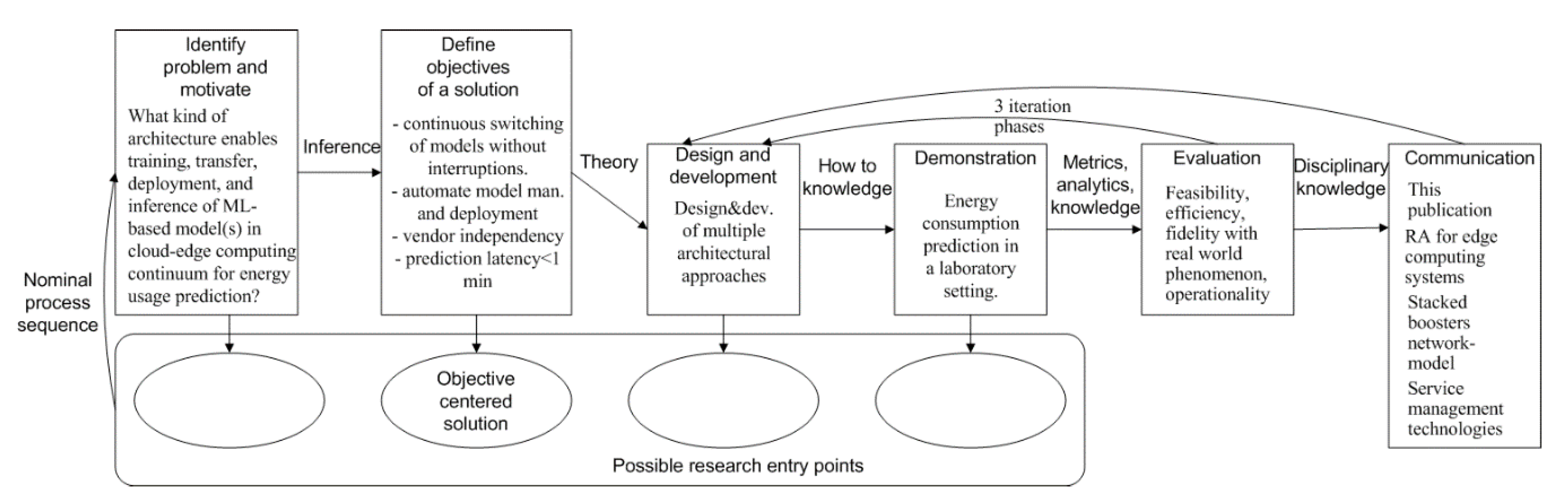
3. Research Method and Process

This research applies the existing Design Science Research Methodology (DSRM) [22]. The research process has been illustrated in Figure 1. The DSRM research process consists of six activities [22]. Initially, a research problem is defined, and the value of a solution is described and motivated. Subsequently, objectives of a solution are specified. Then, an artifact is designed and developed. The artifact can be utilised for demonstrating the solving of the research problem. Evaluation focuses on comparing objectives of a solution to the results obtained with the developed artifact(s) in use. Different evaluation criteria can be used for performing ex-post evaluations [45]. At the end of the evaluation activity, the researcher may iterate back to the design and development activity for improving the performance of the solution. Finally, the problem, artifact(s), and results are communicated to the research community (typically in publications). In the following, our research applying the DSRM is explained in detail.
The initial problem originated from the need to realise energy consumption prediction for building energy management, which should ultimately enable cost savings for building owners the main research problem was:
  • What kind of architecture enables training, transfer, deployment, and inference of ML-based model(s) in cloud-edge computing continuum for energy usage prediction?
Due to the benefits of placing inference in close proximity of buildings (Table 1), an objective was defined for designing, developing, and evaluating an architecture, which enables inference functionality in edge nodes while training the model(s) in the cloud domain. We focused on enabling predictions at edge nodes, and left optimisation of energy consumption for future work. Subsequently, we defined additional objectives for the architecture. First, the architecture should enable continuous training (CI/CD) and switching of models in cloud-edge continuum, which should not lead to interruptions in the prediction service. Model switching is required due to concept drift, which may cause inaccurate predictions with outdated models. Additionally, management and deployment of models should be automatic. Latency of predictions should be less than 1 min, because the frequency of the best smart energy meters has been 1 min [46]. Finally, the architecture should be vendor-independent to avoid locking into company-specific offerings. Our research was objective-centred, because the objectives drove our research process.
The objectives triggered design and development, demonstration, and evaluation phases of the research. Especially, three different architectural approaches were designed, developed, and evaluated regarding feasibility before reaching to the final version of the architecture. Existing knowledge regarding RA for edge computing systems [17], a Stacked Boosters Network-model [23], and service management technologies (Rancher, k3s, Docker) were utilised in the design and development of the architecture. The implemented architectural approaches based on SBN-model and service management technologies can be considered as DSRM-artifacts [22] for solving the research problem. Energy consumption prediction was used as a use case for demonstration and evaluating architectural approaches in a laboratory setting.
Performance of the final architecture version was tested in terms of prediction and model switching latency in edge nodes for evaluation of efficiency. Additionally, the architecture was evaluated in terms of different ex-post criteria [45] (feasibility, efficiency, fidelity with real-world phenomena, operationality of the architecture).

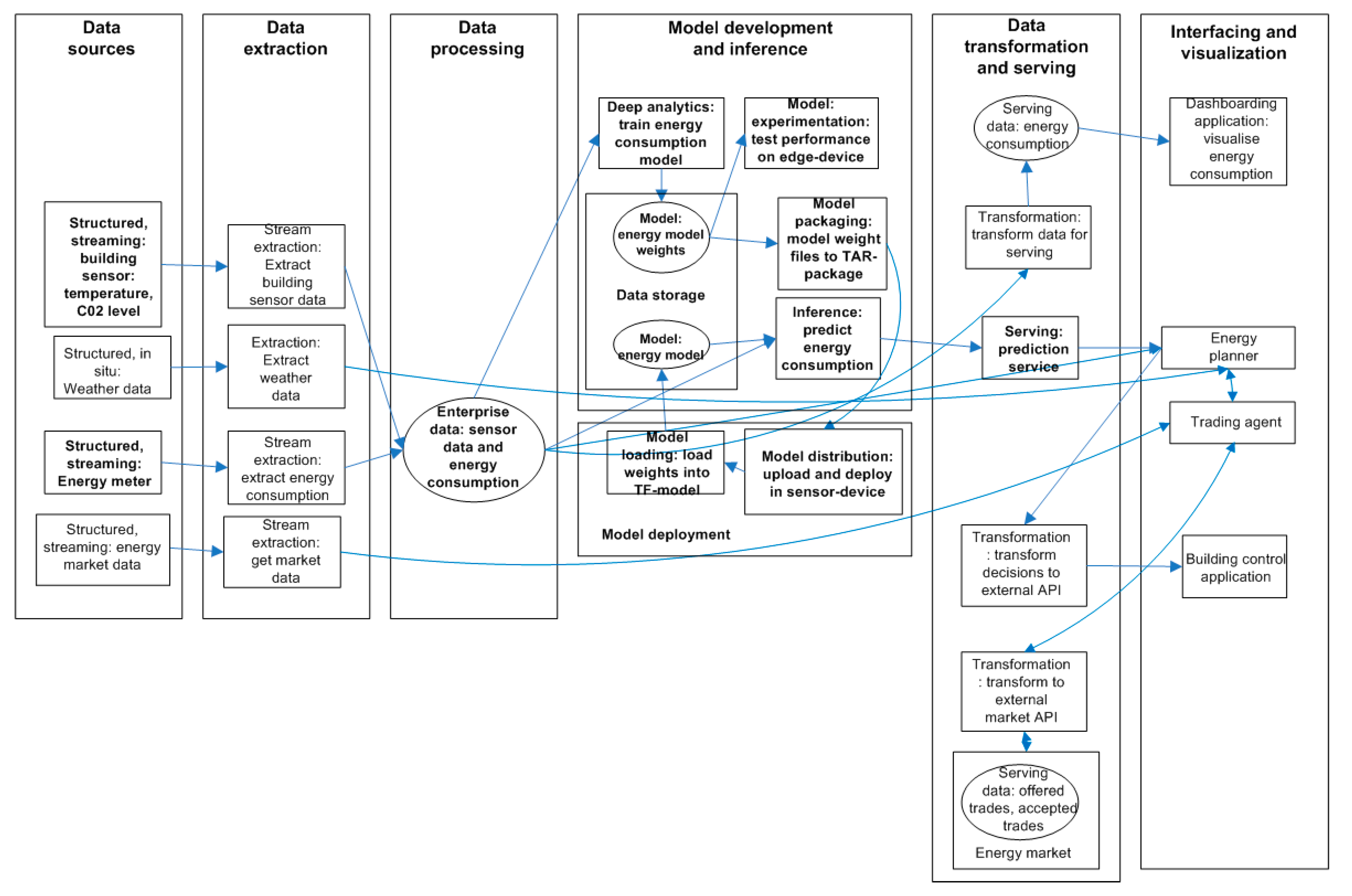
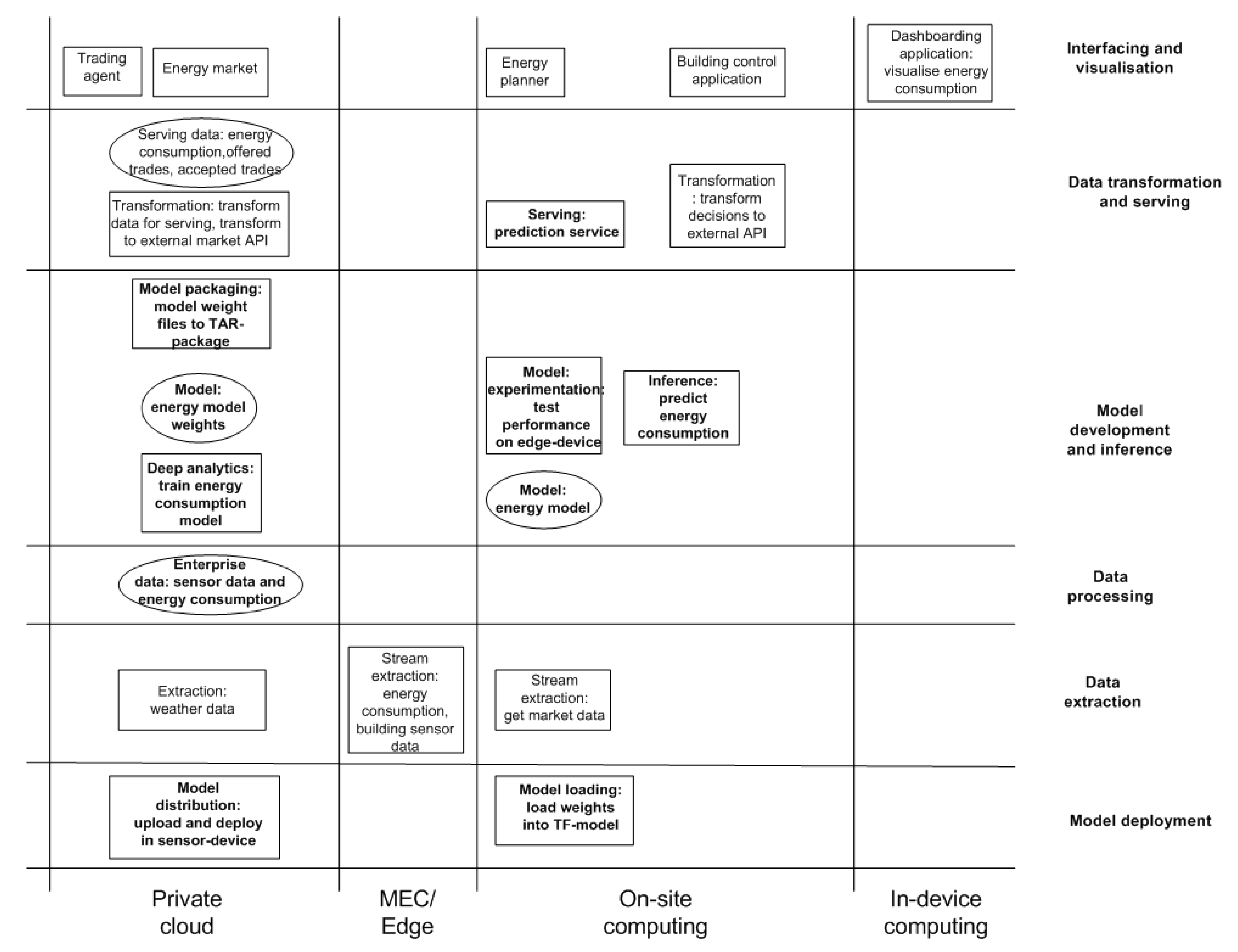
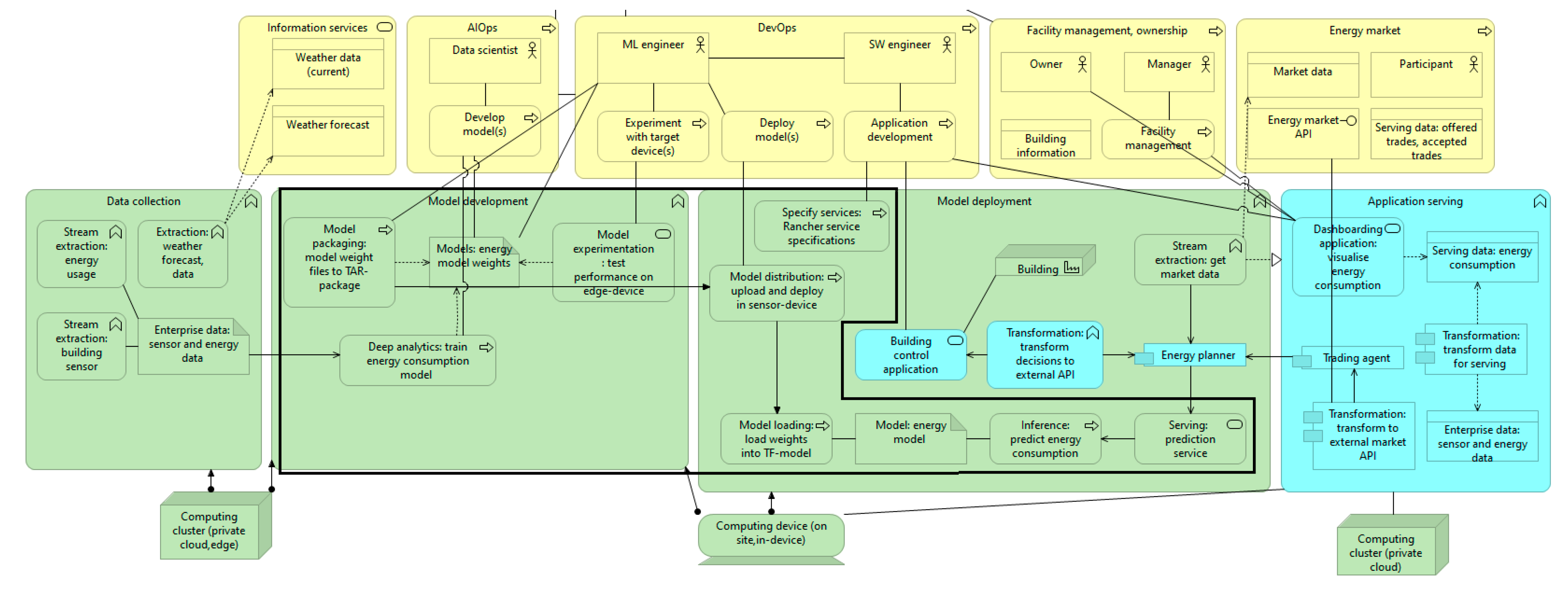
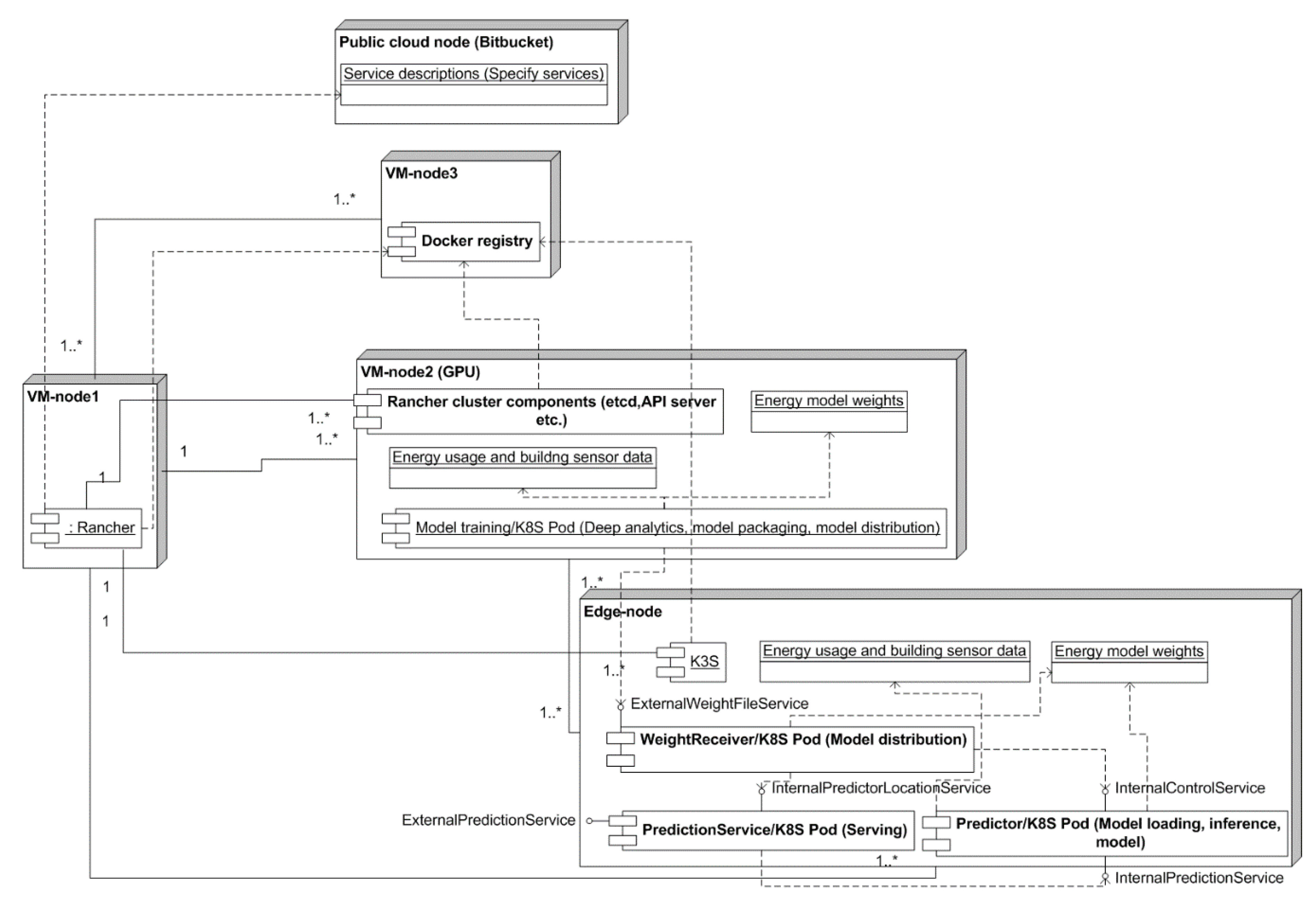
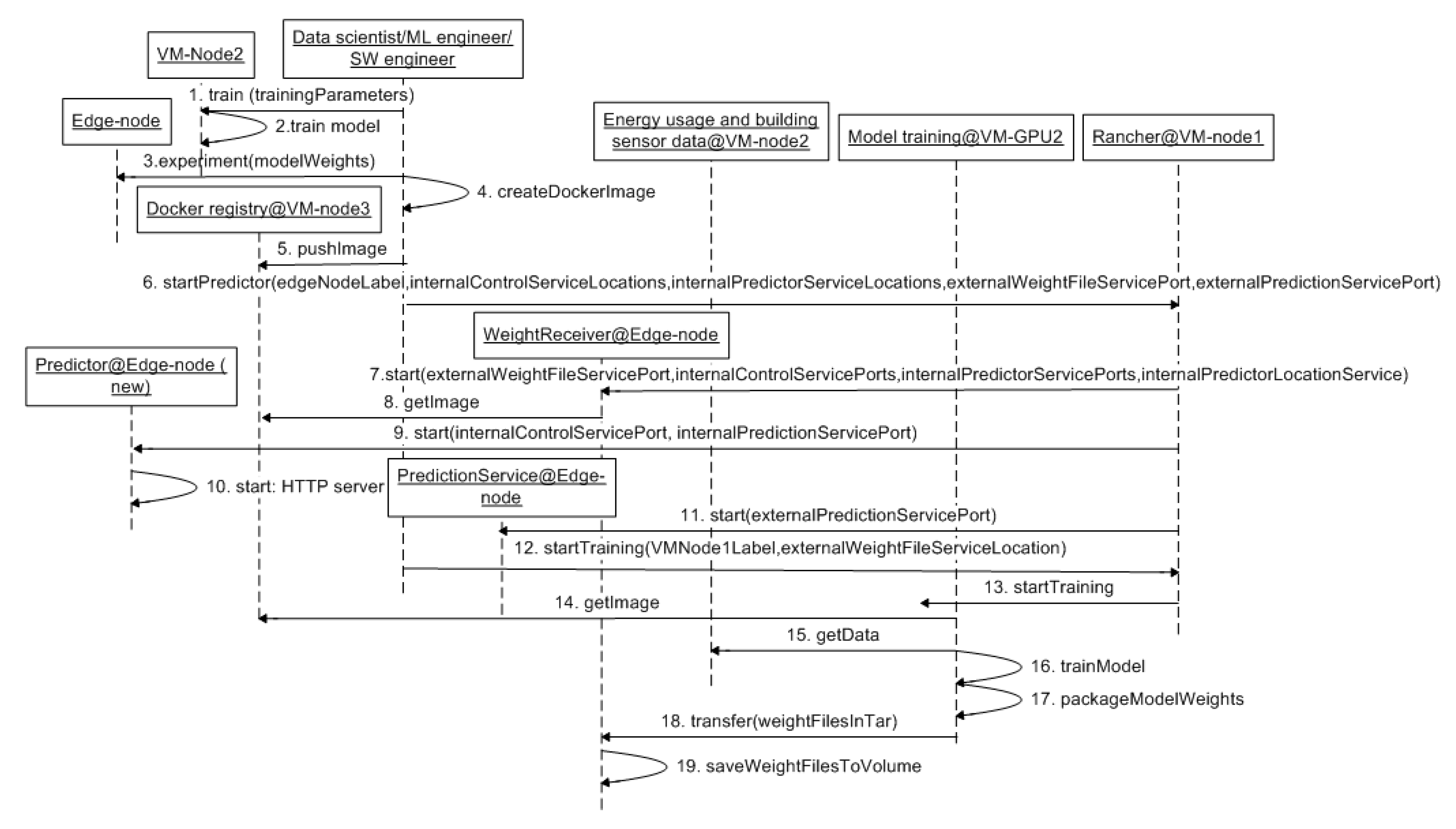
4. Design and Development of the Final Architecture Design

Design and development of the architecture included several phases. The first three phases are described in Appendix D. The results of the initial phases were utilised as a starting point for the design of the final version of the architecture, which is described in this Chapter.
Appendix C presents nodes and main SW components of the prototype system in detail. Especially, HW capabilities of the nodes are described in terms of computing power and memory (in Table A1).

Phase 4: Final Architecture Design

In the following, the design of the architecture is described with several views. Figure 2 provides a high-level data processing view of the architecture. The view was created based on the high-level view of the RA for edge computing systems [17], where ellipsis is used for describing data stores, rectangles illustrate data processing, and arrows describe data flows between architectural elements.
Several data sources may be used within the system. Data may be extracted as a stream from building sensors (e.g., temperature, CO2 level). Energy consumption data of buildings is extracted from energy meters. Other important data sources may include weather data, and associated information about energy markets for trading purposes. In the prototype, sensor and energy consumption data were extracted and saved in an earlier research project into files (Enterprise data) [23]. The data was used for training a model for prediction of energy consumption (Deep analytics). Weights of the model were saved and utilised for performance testing in edge nodes (Model experimentation). After initial experimentation, a mechanism was created for packaging model weight file(s) to a TAR-file (Model packaging), which was transferred to the edge-node (Model distribution). In the edge-node, the files of the package were extracted into the file system, and a new NN-based model was constructed, which the weights were loaded into (Model loading). The model was used for energy consumption prediction of buildings (Inference). A prediction service (Serving) provided responses to requests regarding buildings’ energy consumption.
There are several elements in the architecture, which were not implemented, but are described for providing a better view of the research context. First, energy consumption should be visualised for building owners (Dashboarding application). Energy consumption data may need to be transformed before serving the end users. Additionally, energy consumption predictions should be utilised by an entity (Energy planner), which is able to perform concrete decisions regarding the control of energy devices. Such decisions may need to be transformed prior to executing control commands to actual building control applications. Further, the planned energy consumption information may be utilised for trading in energy markets (Trading agent).
Figure 3 presents a deployment environment view of the architecture, which was designed based on a similar view of the RA for edge computing systems [17]. In the RA, computing devices closest to the data source were considered edge nodes. On-site computing devices were at least one hop closer from the edge nodes towards the point of use. Finally, computing devices, which contained a user interface or an end user application at the point of use, were described in computing devices (e.g., wearables or mobile terminals).
Model training, packaging, and distribution functionalities were deployed in a private cloud (in the prototype), where a VM had access to a powerful GPU (Nvidia Tesla P100 [47]). The trained model was tested and deployed in edge-node(s) (on-site computing environment), where the loaded model was used for prediction of energy consumption in buildings.
Control applications of buildings may be located in close proximity of buildings in order to minimise communication to other domains. Energy consumption may be visualised with mobile terminals to the building owners (in-device computing). Components related to accessing external energy markets may be located within a private cloud.
Figure 4 presents a model development and deployment view, which was designed based on the RA for edge computing systems [17]. Archi-notation [28] was utilised in the design. The view is divided into technological, application, and business layers. Architectural components of the earlier figures (Figure 2 and Figure 3) have been utilised in the design.
First, data was collected in an earlier project [23] from building sensors and energy meters into measurement files (Data collection-function), which was utilised for model training (Deep analytics). Models were trained, packaged, and tested in the Model development-function. AIOps/DevOps could perform the afore-mentioned activities in a real business case. Model deployment-function included model distribution, loading, inference, and serving functionalities. Deployed services in K8S-clusters were managed with Rancher service specifications (Helm [40]). Energy planner would utilise predictions for controlling a buildings energy consumption. Application serving function (not implemented) should contain visualisation of energy consumption for end users (building owners/managers), and possibly trading in energy markets.
Figure 5 presents a Unified Modelling Language (UML) deployment view of the implemented architecture. One VM (VM-node1) was allocated for Rancher, which enabled service management in K8S clusters. Another VM (VM-node2) was allocated for model training. VM-node2 had access to a powerful GPU (Tesla P100) via Nvidia’s drivers. k3s was installed to both edge-nodes (Jetson Nano, RPi 4). RPi 4 acted in a master role in the cluster, and Jetson Nano acted in a worker role. K8S (VM-node2) and k3s-clusters were registered to Rancher. Additionally, a VM (VM-node3) was allocated for running a private Docker registry. Finally, descriptions of services (Helm charts [40]) were uploaded into an external Git (Bitbucket). Git content was imported into Rancher as a new service catalogue [18].
Model training was started from Rancher’s service catalogue to VM-node2. After training was completed, the model weights were packaged into a TAR-file. The file was transferred to the WeightReceiver-component (K8S Pod), which was executed at the edge-node. The component provided a public service interface (ExternalWeightFileService) for receiving packages of new weight files. The weight files were saved into a directory in the local volume (virtualised disk drive). The location of the extracted weight file was provided to the Predictor (K8S Pod) via the internal service (InternalControlService, see the Appendix A for REST API description). After the Predictor had finalised the initialisation of the model, the internal location of the prediction service (InternalPredictionService at the Predictor) was provided to the PredictionService-component (K8S Pod) via the provided service (InternalPredictionLocationService). Finally, PredictionService provided a service interface (ExternalPredictionService, see Appendix A for REST API description) to end users for getting predictions on energy consumption.
Figure 6 presents how models were trained, packaged, and transferred to the edge-node. The steps of the diagram are described as follows:
Steps 1–2: A data scientist/ML engineer starts model training and provides several parameters as input to the process (e.g., hyperparameters). Once training has been finalised, model weights are available for further experimentation.
Step 3: The data scientist/ML engineer may test performance of the model (with weights) in the edge-node. For example, inference latency may be tested.
Steps 4–5: Once initial experimentation with the model has been finalised, the final implementation of the training code is embedded to a Docker image, which is pushed into the private Docker registry.
Step 6: The ML/SW engineer starts Predictor from Rancher’s service catalogue. Several parameters are provided. EdgeNodeLabel indicates the location of the edge-node, where the service will be deployed. The label has been pre-configured (to an IP address) for each registered node in Rancher [18]. Additionally, external ports of WeightReceiver and Predictor-components, and internal service locations of the Predictor-component have to be provided.
Steps 7–8: Rancher starts WeightReceiver based on the provided parameters. Additionally, the internal location of PredictorService-component is provided (InternalPredictorLocationService). The associated Docker image is downloaded from the Docker registry.
Steps 9–10: A Predictor will be started based on the received parameters. The Predictor starts an internal HTTP server for serving prediction requests.
Step 11: The PredictionService is initialised, and the public external port is provided as a parameter.
Steps 12–14: The ML engineer starts model training from Rancher. Label of VM-node1 is provided as a parameter for indicating a node for deployment of the service. Also, the public location of the WeightReceiver-component is provided as a parameter. Finally, the Docker Image is downloaded from the Docker registry.
Steps 15–17: Energy usage and building sensor data is read from internal files. Subsequently, the model is trained, and model weight file is packaged into a TAR-file.
Steps 18–19: The TAR-file is transferred to the WeightReceiver-component (ExternalWeightFileService), and the files are extracted into a volume.
Figure 7 presents model loading based on the received weight file. The view is a continuation of the earlier sequence view (Figure 6). The steps of the view are described as follows:
Step 20: The WeightReceiver-component provides the location of the weight file via the internal control service of the Predictor (see Appendix A for REST API description).
Step 21: The new Predictor provides the received parameter, and an internal port to be utilised for serving of prediction requests.
Step 22: The model is prepared (including loading of weight files into the model).
Step 23: An internal HTTP server is started for serving of prediction requests. Finally, 200 OK HTTP response is returned to the WeightReceiver.
Step 24: The WeightReceiver will update the location of the new Predictor to the PredictionService, after it has received 200 OK response from the new Predictor.
Steps 25–28: The old Predictor will be stopped. HTTP server and Keras/Tensorflow sessions are closed. However, an existing prediction request will be served before closing.

5. Evaluation

5.1. Results of Performance Tests

The purpose of the performance tests was to evaluate the designed architecture in terms of efficiency. Initially, prediction (inference) latency was measured in the edge-nodes. Additionally, the effect of model switching on prediction latency was measured. The executed tests are presented in detail in Appendix B.
The results of the prediction tests are presented in Figure 8. It can be observed that Jetson Nano achieved ~2.2 s lower latency (99th perc. latency= 6.97 s) than RPi 4 (99th perc. latency= 9.16 s).
Figure 9 presents latency of prediction, when a model was switched once per minute. Particularly, new model weights were transferred to edge nodes for switching of a model (see steps 18–28 in Figure 6 and Figure 7), while predictions were provided simultaneously to simulated end users. It can be observed that prediction latency and deviation is higher with both edge-nodes, when the results are compared to prediction without model switching (Figure 8). Figure 10 presents switching latency with both edge-nodes. The switching latency is significantly larger with RPi 4 than with Jetson Nano. Finally, statistics of the tests have been summarised in Table 2. In overall, model switching led to ~2.1–3.7 s increase in prediction latency.

5.2. Feasiblity Evaluation of the Initial (Phases 1–3) Architectural Approaches

Feasibility evaluation results of the first three architectural approaches (see Appendix D) were utilised in the design of the final architecture. The results are summarised in the following:
  • A model created based on NN weights provided feasible predictions in the edge nodes (with a negligible rounding error).
  • Rancher pipelines [18] was not feasible due to an unresolved error in the Docker image building phase (error was related to updating of pip).
  • 64-bit OS version (Ubuntu 20.04 in RPi4) in the edge nodes was compatible with k3s.
  • Predictors have to be placed into separate K8S pods in order to achieve uninterrupted operation of prediction services, when a ML-based model is updated in the edge node.

5.3. Evaluation of the Final Architecture Design

5.3.1. Feasibility

The following implementation-related lessons were learnt regarding feasibility of the final architecture design:
  • NFS server was tested for storing of model weight files. The integration between Rancher and NFS server was performed successfully with K8S Persistent Volume Claims [48]. However, k3s didn’t provide support for a NFS client. Thus, the received weight files were stored locally to the edge-node, and Rancher’s Local Path Provisioner [18] was utilised for accessing of the files.
  • Initially, Docker images for ARM-devices (Jetson Nano, RPi 4) were built with a laptop, which contained Ubuntu VM in a VirtualBox. Docker images were compiled with Docker’s buildx-tool [49], which is an experimental feature in Docker. However, it was discovered that building of the images was too slow as images couldn’t be built within a working day. Thus, Docker images for ARM-devices had to be built with Jetson Nano.
  • Nvidia has published base images including Tensorflow libraries to be used for building of Docker images for ARM-devices based on Nvidia’s libraries [50]. The Docker image for Jetson Nano was built based on Nvidia’s base image (l4t-tensorflow:r32.4.3-tf1.15-py3), which contained Tensorflow v1.15. However, RPi 4 does not support Nvidia’s libraries. The authors could not find official Docker images, which would contain Tensorflow libraries for RPi. Thus, an unofficial Tensorflow image [51] was used as a base image for RPi 4.
  • In order to get access to GPU-resources, Docker’s default runtime had to be changed to ‘nvidia’ in Jetson Nano. Additionally, k3s uses contained as the default container runtime, which had to be changed to Docker in order to get access to GPU resources via Nvidia’s libraries.
The SBN-implementation [23] was utilised for energy consumption prediction in the architecture. Model weights of a trained model (trained with the SBN-implementation) were transferred in a file to the edge nodes. Additionally, data had to be available in the edge node for scaling input data similarly, which was performed during training. Model conversion/saving to a file may have been a better option, which would not have required the presence of training data in the edge node(s). However, model conversion was not feasible due to an error, which was encountered during model saving (see Phase 1 in Appendix D).
Feasibility of the architecture may be evaluated in terms of the RA it is based on, and the applied technological choices. Three architectural views of the RA for edge computing systems [17] were applied as a starting point in the design of the presented implementation architecture (Figure 2, Figure 3 and Figure 4). The implemented architecture was designed based on the elements of the RA. However, the RA could be evaluated only partly, as all elements of the RA were not covered by the prototype. For example, data extraction was performed in an earlier project [23], and visualisation and interfacing-related elements were not implemented. Similarly, only model development and deployment technological layers of the Archimate-view could be evaluated in this paper. We presented the unimplemented architectural elements, due to their importance for understanding the context of energy consumption prediction in facilities.

5.3.2. Efficiency

Latency of prediction was quite high. The factors behind the low performance were studied further. It was discovered that parsing of a JSON-request to a Python Dataframe took ~40–80 ms (an input request contained 600 data samples with a timestamp and temperature (Appendix A)). The rest of the delay (~6–9 s) consisted of getting predictions from the SBN-model [23]. Within the chosen research context, the observed latency was feasible, because the frequency of energy consumption data from the best smart meters has been 1 min [46]. Thus, predictions can be provided for realising energy consumption optimisation (in the future) within the performance requirement (1 min). However, SBN-model prediction latency should be reduced in future work.
With the presented model switching mechanism (Figure 7) predictions could be provided simultaneously from the old model during the loading of a new model. Performance results (Figure 9) indicated that model switching increased prediction latency by ~2.1–3.7 s. However, the increased latency is below the performance requirement (1 min). Without the implemented model switching mechanism, serving of prediction requests would have been interrupted (at least) for the duration of model loading in the new predictor (due to closing of Keras/Tensorflow session of the old predictor; see Appendix D; phase 3). Further tests with Jetson Nano indicated ~21–22 s model loading latency.
In reality models may be switched much less often (e.g., few times per day/week), because the frequency of the best smart energy meters is 1 min [46]. Thus, the results present an extreme situation, where models are switched more often than may actually be needed.

5.3.3. Fidelity with Real World Phenomenon

Energy consumption optimisation of buildings is the ultimate goal of our work. Particularly, we enabled predictions in edge-nodes, which could be located in buildings. Realising of energy consumption optimisation is left for future work.
Implementation of energy consumption optimisation in the real world depends on the feasibility of the architecture and applied technologies (see Section 5.3.1). The main technologies may be additionally analysed in terms of industry adoption. K8S has become the de-facto technology for running workloads in computing clusters. Rancher is vendor independent (a solution objective; Figure 1). Particularly, Rancher is open source and does not lock users into vendor-specific solutions [18]. Both Rancher and k3s are utilised increasingly in the industry [18].

5.3.4. Operationality

Prediction feasibility was initially tested by comparing predictions after training, and after model loading with an edge-node (Phase 1 in architecture design and development; Appendix D). UML sequence diagrams (Figure 6 and Figure 7) describe functionality of the architecture, which included model switching without interrupting inference services to end users. Particularly, it was illustrated how models are trained, weights are packaged, transferred, and deployed to edge nodes. Finally, prediction feasibility was ensured in the final architecture, which was implemented.

6. Discussion

The results can be compared to related work. The RA [17] was evaluated in this work for realising an implementation architecture in the context of energy consumption prediction for facilities. The earlier work did not focus on evaluation [17], and this work may be considered as one step toward evaluating the RA. A similar mapping between the earlier version of our RA [52] and an implementation architecture has been performed for a system focusing on anomaly detection on power consumption [53]. Their work covered all functional areas of the RA [52], which was not covered by this work for the newer version of the RA [17]. However, the major differences between the RAs [17,52] is in ‘Model development and inference’ and ‘Model deployment’ FAs, which were focused in this work. Other RA proposals are also available for edge computing systems, which have been compared to our proposal earlier [17].
We relied on the utilisation of container implementations (Docker in Jetson Nano and contained in RPi 4) in each of the edge nodes, which may add some overhead to edge-nodes. However, earlier research has shown that Docker has negligible effect on the performance (<5%) in edge nodes [11]. DLASE [43] packaged ML-models into Docker images, which were transferred via REST API to edge nodes (with enhanced OpenBalena), and models were deployed with Tensorflow Serving. Instead of deploying pre-configured models [43], we focused on updating of the predictors based on new weight files. Also, we managed Docker-based services in Kubernetes clusters with Rancher instead of using OpenBalena [43].
Several approaches have been proposed in the literature for improving the performance of inference in cloud-edge continuum [33,34,35,36,37]. The main difference is that we do distribute inference between nodes in cloud-edge continuum, due to the argued benefits of our approach (Table 1). Li et al. [21] proposed an interesting architecture for enabling container-based continuous training and deployment of models in the context of optimising energy consumption in power plants. A major difference between the architectures is our focus on placing model training to the private cloud, and inference to the resource-constrained edge nodes. On the contrary, Li et al. had placed both functionalities to powerful servers with GPU-cards. Additionally, we executed functionalities in K8S clusters and integrated with Rancher for service management, whereas Li et al. focused on execution in Docker containers. They also implemented a similar model switching mechanism, which can be compared to our proposal. The difference is that their broker queries master/slave instances of models for determining, which model instance can be utilised for providing a response. We decided to keep the broker/service always up-to-date regarding the location of the model instance, which is able to provide predictions. Their proposal reaches low latency (~100–150 ms) in prediction, and model switching had a small effect on the latency. We analysed the factors of high prediction latency earlier (in terms of efficiency; see Section 5.3.2), which should be focused on in future work.
Functionality related to continuous model training and transfer of models to edge nodes is associated with DevOps [14], ModelOps [15] and AIOps [29] concepts. ModelOps is a platform for management and improvement of AI application artifacts, while AIOps refers to empowering SW/service engineers for addressing the challenges associated to the utilisation of AI/ML techniques [17]. The afore-mentioned concepts have been taken into consideration in the RA [17], which was utilised as a basis for the design of our system view (Figure 4). However, feasibility of the architecture should be evaluated in the future in a real SW development project with actors in suitable AIOps/DevOps roles.
Comparison to related work indicates novelty of the presented architecture for predicting energy consumption in cloud-edge continuum. Especially, it is argued that a combination of the chosen technologies (Rancher, k3s, Docker) has not been experimented in environments consisting of a private cloud and edge nodes for prediction of facilities’ energy consumption. Several implementation-related lessons were learnt during the implementation work. Another contribution is partial evaluation of the RA for edge computing systems [17] with the presented prototype system.
As our contribution focused on enabling energy consumption prediction in edge nodes, future work should focus on realising energy consumption optimisation based on the predictions. For example, economic savings for building owners may be realised by shifting energy loads at peak times based on the predictions [10]. Additionally, decision making on energy consumption optimisation, frequency of model updates, and integration to buildings’ energy control interfaces (e.g., HW/SW interfaces) should be focused on. Also, cost of edge devices (including network connection) should be analysed for evaluating commercialisation of the solution.
Finally, it should be mentioned that the evaluation of the RA [11] is biased by our familiarity with the RA design [17]. Particularly, we didn’t observe a learning curve related to the adoption of the RA [54], when the RA was utilised as a basis of the implementation architecture design. This may have affected reliability of the research. For example, a research scientist who is unfamiliar of the RA may perform different design choices due to the learning curve associated with the adoption of the RA, if the study would be repeated. However, our design should be considered at least as an example, how the RA [17] could be evaluated in the future by others.

7. Conclusions

This paper focused on architecture design for predicting facilities’ energy consumption in a cloud-edge continuum. The study was performed by applying the Design Science Research Methodology. Particularly, the research question was related to architecture design, which enables ML-based inference in edge-nodes while performing model training within the private cloud. Subsequently, objectives for the architecture were specified. A Reference Architecture for edge computing systems was utilised as a starting point for the design of the implementation architecture. Different architectural approaches were designed, implemented, and evaluated in multiple phases of the study. Architecture design of the final version of the implemented system was presented from several viewpoints. Performance of the prototype system was tested regarding latency of inference and model switching. Finally, the architecture was evaluated against specified criteria. Rancher and k3s were feasible for management of K8S-based services in cloud-edge continuum, while the SBN-implementation enabled energy consumption prediction in the edge nodes. Efficiency of the solution in terms of prediction latency (~7–9 s) was low (but acceptable to the research context) due to delay associated with model inference. Additionally, a mechanism for continuous switching of prediction models in edge nodes was implemented. Switching of the models led to an increased latency (~9–13 s), when simultaneously serving prediction requests. Operationality of the architecture was visualised with several architectural views, and by ensuring feasibility of edge node predictions.
The RA was utilised successfully in the design of the concrete system architecture. Comparison to related work indicated novelty of the applied technologies (Rancher, k3s, Docker) in the chosen research context. Partial evaluation of the Reference Architecture with the prototype system may be considered as an additional contribution.
Future work may include improvement of the SBN-model [23] for enabling saving and conversion of the prediction model into compressed files (e.g., TFLite-format [55]), optimisation of inference performance in the edge nodes, design, and development of components utilising energy consumption predictions for energy management of buildings, and evaluation of the architecture in a real development project with actors in AIOps/DevOps roles.

Author Contributions

Conceptualisation, P.P. and D.P.; methodology, P.P. and D.P.; software, P.P.; validation, P.P., D.P., R.S. and J.K.; investigation, P.P.; resources, P.P. and D.P.; data curation, P.P.; writing—original draft preparation, P.P. and D.P.; writing—review and editing, P.P., D.P, and J.K.; supervision, D.P. and J.K.; project administration, D.P.; funding acquisition, D.P. All authors have read and agreed to the published version of the manuscript.

Funding

This research was funded by VTT Technological Research Centre of Finland.

Conflicts of Interest

The authors declare no conflict of interest.

Appendix A

In the following, selected service interfaces of the prototype systems are presented. ExternalPredictionService enabled the querying of predictions based on input consisting of hourly timestamps and temperature readings.
REST API: ExternalPredictionService:
Request: HTTP POST with JSON payload
{
 “Request”: “PredictEnergyUsage”,
 “DataPoints”: {
  “2012-02-23 10:00:00”: {
   “Temperature”: “0.4”,
   “EnergyUsage”: “160”
  },
  “2012-02-23 11:00:00”: {
   “Temperature”: “0.5”,
   “EnergyUsage”: “166”
  }
 }
}
Response: HTTP 200 OK with JSON payload
{
 “Response”: “PredictedEnergyUsage”,
 “DataPoints”: {
  “2012-02-23 10:00:00”: {
   “EnergyUsage”: “160”
  },
  “2012-02-23 11:00:00”: {
   “EnergyUsage”: “166”
  }
 }
}
InternalControlInterface of the Predictor enabled starting and stopping of a Predictor based on received weight file(s). The location of the weight file(s) was indicated to the Predictor, when a Predictor was started.
REST API: InternalControlInterface:
Request: HTTP POST with JSON payload
{
 “Request”: “StartPredictor/StopPredictor”,
 “WeightFileLocation”: “/fdf/dsds/”
}
Response: HTTP 200 OK with JSON payload
{
 “Response”: “OK/Failed”
}

Appendix B

In the following, the executed performance tests are described. Duration of both experiment was 3 h.
Prediction inference tests:
  • The edge-node was booted.
  • A Docker image was built in the edge node, and a weight file was included into the image.
  • A Docker container was started based on the Docker image. A model was created based on the weight file.
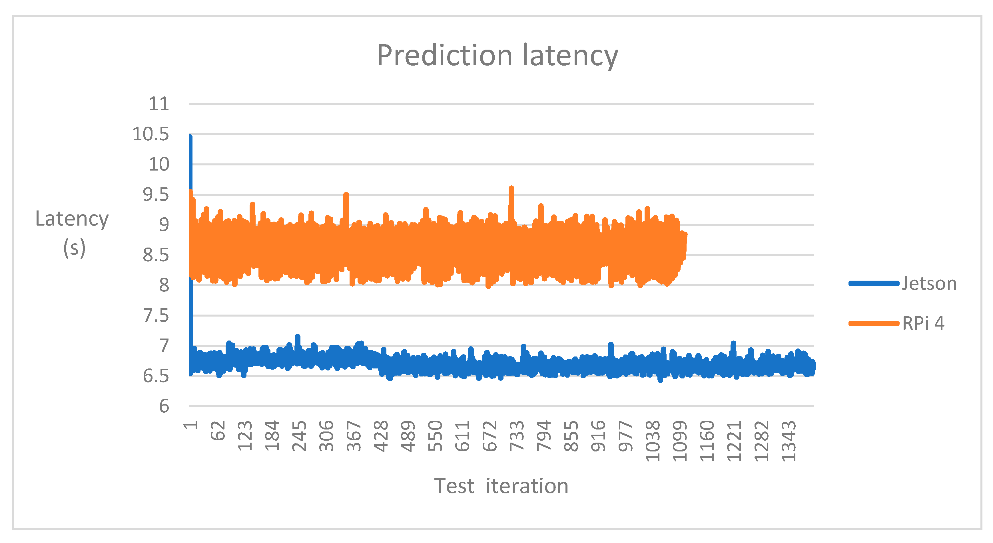
  • A wget() loop was used for getting predictions (predictions for ~2.6 days; 62 hourly predictions). Each request consisted of 600 data points (~3 weeks of input data). The loop slept 1 s after completion of a request.
  • Latencies were extracted into a file based on the terminal output.
Model switching tests:
  • The Edge-node was booted.
  • Predictor components (Figure 5) were deployed to the edge-node from Rancher’s service catalogue.
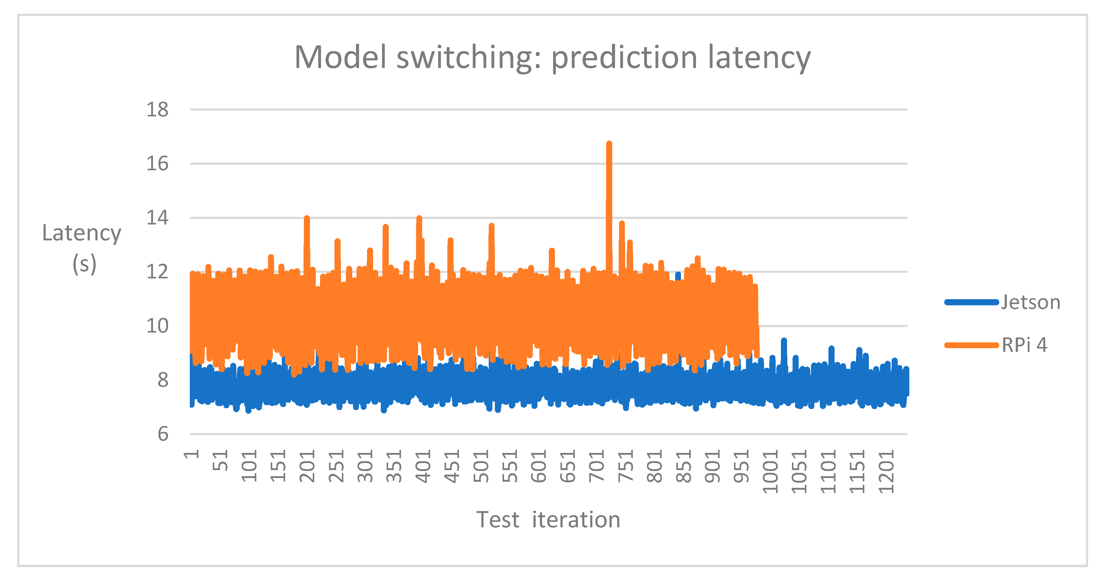
  • A loop was started, which transferred a new weight file to the edge-node once per minute (by utilising ExternalWeightFileService in Figure 5).
  • Another loop was started for requesting predictions (similar loop as step 4 in the prediction inference tests).
  • Latencies of both loops were extracted into a text file based on the terminal output.

Appendix C

HW capabilities of the nodes in the prototype system are presented in Table A1. Table A2 presents SW components, and the nodes utilised for execution.
Table A1. HW capabilities of the nodes in terms of memory, CPU and GPU/CUDA cores.
NodeMemory (GB)CPU (cores)GPU (CUDA Cores)
VM-node1 (Rancher)403x
VM-node2 (GPU)197 12 3584
Jetson Nano44128
RPi 444x
Table A2. SW component versions and nodes, where the components were executed in.
SW ComponentVersionNode
Rancher2.4.7VM-node1
Kubernetes-k3s1.18.8Jetson Nano, RPi 4
Kubernetes-VM1.18.6VM-node1, VM-node2
Tensorflow1.14–1.15VM-node2, Jetson Nano, RPi4
Keras2.2.0VM-node2, Jetson Nano, RPi4

Appendix D

This appendix contains design, implementation and evaluation of the initial design phases of the architecture.

Appendix D.1. Phase 1: Feasibility of Predictions in Edge-Nodes

The existing SBN-implementation [23] was utilised for predicting energy consumption in buildings. The initial approach was to save the SBN-model into a file, which could be loaded into memory at the edge-node(s). However, due to the way the earlier implementation was constructed, the model couldn’t be saved into a file. Thus, an alternative approach was chosen for transferring the model to the edge node(s). Weights of the trained NN model were saved, and transferred to the edge-node(s), where the NN-based model was constructed based on the weight file(s). The goal of the experiment was to ensure that the loaded model provides valid predictions in the edge node(s). In the design (Figure A1), ellipsis is used for describing data stores, rectangles illustrates data processing, and arrows describe data flows between architectural elements (a similar notation was used in the RA [17]).
A demonstration was performed based on the following steps:
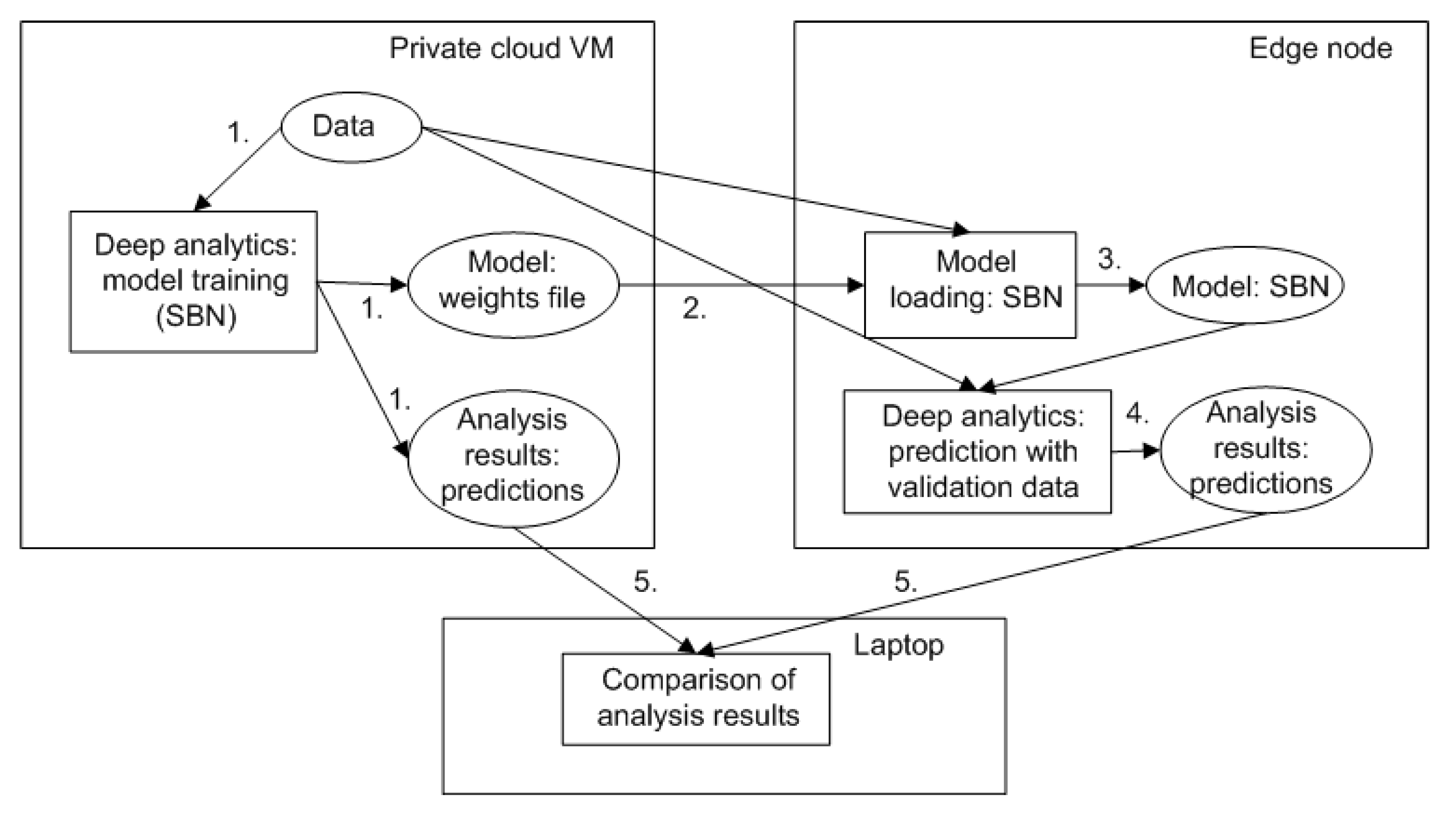
  • SBN model(s) were trained in the private cloud based on several existing datasets [23]. After each training phase, weights of the trained model were saved into a file. Additionally, predictions were produced based on validation data (energy consumption prediction for 3 weeks) and saved.
  • The weight files were transferred to the edge-node.
  • A prediction model was created based on the loaded weight file(s) in the edge-node. Additionally, training data was needed in the edge-node to perform similar scaling of features, which was performed during the training phase.
  • Predictions were performed in the edge node (based on validation data) and saved.
  • The predictions after training (step 1) and after reloading of the model in the edge-node (step 4) were compared to ensure feasibility of the approach.
Figure A1. Architecture design for evaluating feasibility of predictions in edge nodes.
Futureinternet 13 00005 g0a1
Feasibility evaluation:
  • In most cases, the loaded model in edge node produced the same predictions as the original model in the private cloud. However, in ~2.7% of the predictions, there was a rounding error (10−5) which is negligible. Thus, the chosen architectural approach for model training, transfer, and model loading was feasible for further design of the architecture.

Appendix D.2. Phase 2: Automation of ML-Based Model Management and Deployment with Rancher Pipelines

Rancher pipelines [18] enable CI/CD of code into production. Rancher pipelines was integrated with the SBN-implementation [23] for enabling automatic creation of Docker images. The demonstration was executed as follows (Figure A2):
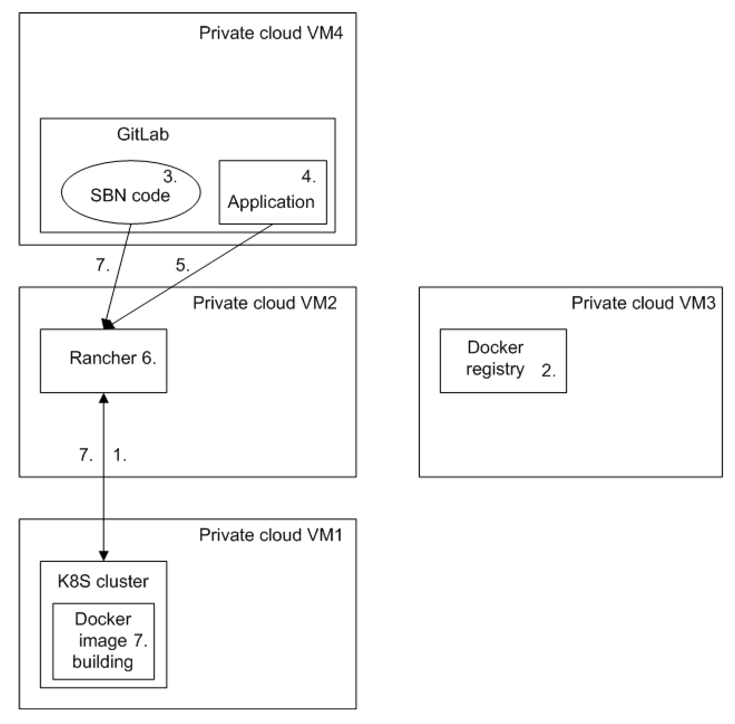
  • A K8S cluster was created to a Virtual Machine (VM) (VM1) in the private cloud. The cluster was registered into Rancher (VM2).
  • Docker registry [56] was initialised to another VM (VM3) in the private cloud for storing of Docker images.
  • Code of the existing SBN-implementation was published in GitLab (VM4). A Dockerfile was added to the code base for building a Docker image based on the code.
  • An application was added to GitLab for integration with Rancher.
  • The GitLab-application was authenticated with Rancher (Tools/Pipeline).
  • A pipeline was added into the K8S-cluster with Rancher. Location of the Dockerfile and Docker registry were provided.
  • Building of the Docker image was triggered from Rancher UI, or based on a Git commit to GitLab. The SBN-implementation was downloaded from GitLab, and placed into the K8S-cluster for building.
Figure A2. Architecture design for continuous integration/delivery with Rancher pipelines.
Futureinternet 13 00005 g0a2
Feasibility evaluation:
  • Building of the Docker image based on the SBN-implementation (at GitLab) was triggered successfully based on the Git commit. However, the Docker image could not be built due to an error encountered in building. Particularly, the latest version of pip could not be installed, and Docker image creation stopped.
  • It was concluded that Rancher pipelines may be utilised for CI/CD of code, but the feature was not applicable for our purpose. Thus, we decided to proceed without Rancher pipelines for further development.

Appendix D.3. Phase 3: Continuous Training and Switching/Updating (CI/CD) of ML-Based Model(s)/Uninterrupted Operation of Prediction Services: Multi-Threaded Predictors in a K8S Pod

An architecture was designed for a system, in which multiple (2) predictors (running in separate threads) were placed within a K8S Pod (Figure A3). With this approach, a predictor was loaded/updated based on a weight file, which had been trained earlier. Also, the old predictor (created based on an old model weight file) was deactivated. The following experiments were executed:
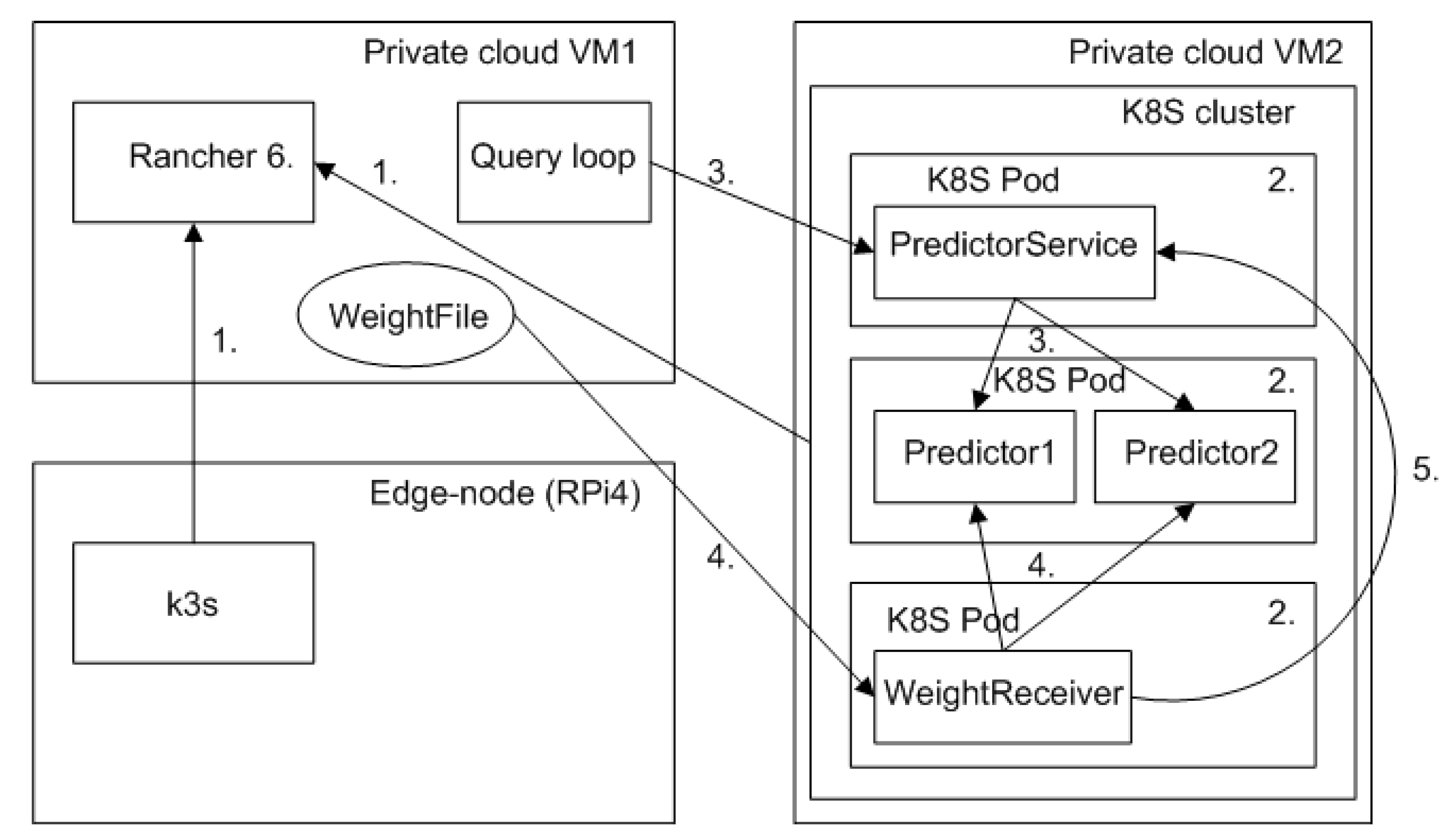
  • Two K8S clusters were created and registered to Rancher (VM1). One cluster was running in the private cloud (VM2). The other k3s cluster was executed in the edge node (RPi 4).
  • The architecture consisting of multi-threaded predictors, a weight receiver, and a prediction service was placed to the K8S cluster of the private cloud (VM2).
  • The predictor was queried for energy consumption prediction from the predictor service, which forwarded queries to the active predictor.
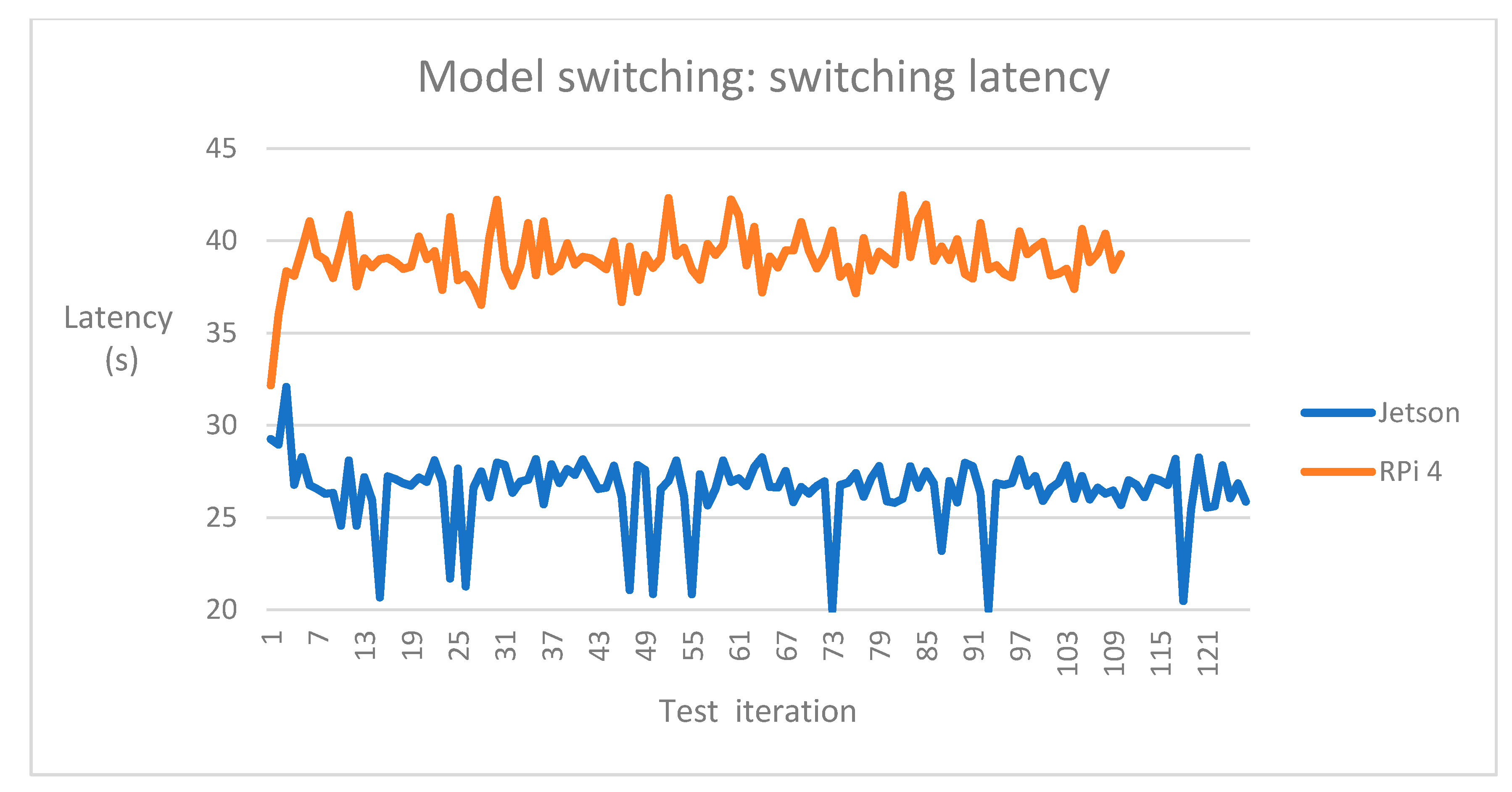
  • Model switching was experimented by transferring new weight files to a weight receiver, which managed switching of the predictors. Each time a new weight file was received, the inactive predictor was loaded with a new weight file, and the old predictor was deactivated.
  • Location of the active predictor was updated to the prediction service.
Figure A3. Architecture design for multi-threaded predictors in a K8S-Pod.
Futureinternet 13 00005 g0a3
Feasibility evaluation:
  • First, a 64-bit OS (Ubuntu 20.04; aarch64) had to be installed to RPi 4 in order to be compatible with k3s (32-bit Raspbian installation wasn’t compatible with k3s; See the issue in k3s GitHub [57]). After the installation of Ubuntu 20.04 in RPi 4, the k3s cluster was registered successfully to Rancher.
  • It was discovered that a Keras/Tensorflow-session of the old predictor had to be closed, before the new predictor could be initialised successfully. Thus, predictions couldn’t be provided to end users from the old predictor during the switching operation. This caused an additional delay to the provisioning of predictions. Based on the discovery, it was decided to place predictors to separate K8S Pods in further design of the architecture.

References

  1. Annual Energy Outlook Early Release. Energy Information Administration (EIA). Available online: https://www.eia.gov/outlooks/aeo/ (accessed on 18 November 2020).
  2. Rousselot, M. ODYSSEE-MURE Policy Brief: Energy Efficiency Trends in Buildings. Available online: https://www.odyssee-mure.eu/publications/policy-brief/buildings-energy-efficiency-trends.html (accessed on 18 November 2020).
  3. Heating Cooling. Available online: https://ec.europa.eu/energy/topics/energy-efficiency/heating-and-cooling_en (accessed on 18 November 2020).
  4. Ruelens, F.; Iacovella, S.; Claessens, B.J.; Belmans, R. Learning agent for a heat-pump thermostat with a set-back strategy using model-free reinforcement learning. Energies 2015, 8, 8300–8318. [Google Scholar] [CrossRef] [Green Version]
  5. Barrett, E.; Linder, S. Autonomous hvac control, a reinforcement learning approach. In Proceedings of the Joint European Conference on Machine Learning and Knowledge Discovery in Databases, Porto, Portugal, 7–11 September 2015. [Google Scholar]
  6. Jia, R.; Jin, M.; Sun, K.; Hong, T.; Spanos, C. Advanced building control via deep reinforcement learning. Energy Procedia 2019, 158, 6158–6163. [Google Scholar] [CrossRef]
  7. Zhang, Z.; Chong, A.; Pan, Y.; Zhang, C.; Lu, S.; Lan, K.P. A Deep Reinforcement Learning Approach to Using Whole Building Energy Model for HVAC Optimal Control. In Proceedings of the Building Performance Modeling Conference and SIMBuild, Chicago, IL, USA, 26–28 September 2018. [Google Scholar]
  8. Afram, A.; Janabi-Sharifi, F.; Fung, A.S.; Raahemifar, K. Artificial neural network (ANN) based model predictive control (MPC) and optimization of HVAC systems: A state of the art review and case study of a residential HVAC system. Energy Build. 2017, 141, 96–113. [Google Scholar] [CrossRef]
  9. Jain, A.; Smarra, F.; Reticcioli, E.; D’Innocenzo, A.; Morari, M. NeurOpt: Neural network based optimization for building energy management and climate control. In Proceedings of the 2nd Annual Conference on Learning for Dynamics and Control, Berkeley, CA, USA, 11–12 June 2020; pp. 445–454. [Google Scholar]
  10. Zhou, B.; Li, W.; Chan, K.W.; Cao, Y.; Kuang, Y.; Liu, X.; Wang, X. Smart home energy management systems: Concept, configurations, and scheduling strategies. Renew. Sustain. Energy Rev. 2016; 61, pp. 30–40. [Google Scholar]
  11. Hadidi, R.; Cao, J.; Xie, Y.; Asgari, B.; Krishna, T.; Kim, H. Characterizing the Deployment of Deep Neural Networks on Commercial Edge Devices. In Proceedings of the IEEE International Symposium on Workload Characterization (IISWC), Orlando, FL, USA, 3–5 November 2019. [Google Scholar]
  12. Chen, J.; Ran, X. Deep learning with edge computing: A review. Proc. IEEE 2019, 107, 1655–1674. [Google Scholar] [CrossRef]
  13. Pakkala, D.; Spohrer, J. Digital Service: Technological Agency in Service Systems. In Proceedings of the Hawaii International Conference on System Sciences, Honolulu, HI, USA, 8–11 January 2019. [Google Scholar]
  14. Wiedemann, A.; Forsgren, N.; Wiesche, M.; Gewald, H.; Krcmar, H. Research for practice: The DevOps phenomenon. Comm. ACM 2019, 62, 44–49. [Google Scholar] [CrossRef] [Green Version]
  15. Hummer, W.; Muthusamy, V.; Rausch, T.; Dube, P.; El Maghraoui, K.; Murthi, A.; Oum, P. ModelOps: Cloud-based lifecycle management for reliable and trusted AI. In Proceedings of the IEEE International Conference on Cloud Engineering (IC2E), Prague, Czech Republic, 24–27 June 2019. [Google Scholar]
  16. Sittón-Candanedo, I.; Alonso, R.S.; Corchado, J.M.; Rodríguez-González, S.; Casado-Vara, R. A review of edge computing reference architectures and a new global edge proposal. Future Gener. Comput. Syst. 2019, 99, 278–294. [Google Scholar] [CrossRef]
  17. Pääkkönen, P.; Pakkala, D. Extending reference architecture of big data systems towards machine learning in edge computing environments. J. Big Data 2020, 25, 1–29. [Google Scholar] [CrossRef] [Green Version]
  18. Rancher. Available online: https://rancher.com/ (accessed on 18 November 2020).
  19. k3s-Lightweight Kubernetes. Available online: https://rancher.com/docs/k3s/latest/en/ (accessed on 18 November 2020).
  20. Luo, H.; Cai, H.; Yu, H.; Sun, Y.; Bi, Z.; Jiang, L. A short-term energy prediction system based on edge computing for smart city. Future Gener. Comput. Syst. 2019, 101, 444–457. [Google Scholar] [CrossRef]
  21. Li, K.; Gui, N. CMS: A Continuous Machine-Learning and Serving Platform for Industrial Big Data. Future Internet 2020, 12, 102. [Google Scholar] [CrossRef]
  22. Peffers, K.; Tuunanen, T.; Rothenberger, M.A.; Shatterjee, S. A Design Science Research Methodology for Information Systems Research. J. Manag. Inf. Syst. 2007, 24, 45–77. [Google Scholar] [CrossRef]
  23. Salmi, T.; Kiljander, J.; Pakkala, D. Stacked Boosters Network Architecture for Short-Term Load Forecasting in Buildings. Energies 2020, 13, 2370. [Google Scholar] [CrossRef]
  24. ISO/IEC JTC1/SC 42 Committee. Available online: https://www.iso.org/committee/6794475.html (accessed on 18 November 2020).
  25. Big Data Value Association. BVA SRIA—European Big Data Value Strategic Research and Innovation Agenda. Available online: http://bdva.eu/sites/default/files/BDVA_SRIA_v4_Ed1.1.pdf (accessed on 18 November 2020).
  26. Chang, W.L.; Boyd, D.; Levin, O. NIST Big Data Interoperability Framework: Volume 6, Reference Architecure. NIST Big Data Program. Available online: https://www.nist.gov/publications/nist-big-data-interoperability-framework-volume-6-reference-architecture (accessed on 18 November 2020).
  27. Lin, S.; Simmon, E. The Industrial Internet of Things Volume G1: Reference Architecture; Industrial Internet Consortium: Needham, MA, USA, 2019. [Google Scholar]
  28. ArchiMate 3.1 Specification. The Open Group. Available online: https://pubs.opengroup.org/architecture/archimate3-doc/ (accessed on 18 November 2020).
  29. Dang, Y.; Lin, Q.; Huang, P. AIOps: Real-World challenges and research innovations. In Proceedings of the IEEE/ACM 41st International Conference on Software Engineering: Companion Proceedings (ICSE-Companion), Montreal, QC, Canada, 25–31 May 2019. [Google Scholar]
  30. Galster, M.; Avgeriou, P. Empirically-grounded reference architectures: A proposal. In Proceedings of the Joint ACM SIGSOFT Conference on Quality of Software Architectures and ACM SIGSOFT Conference on Quality of Software Architectures and ACM SIGSOFT Symposium on Architecting Critical Systems, Boulder, CO, USA, 20–24 June 2011. [Google Scholar]
  31. Hardy, C.; Merrer, E.L.; Sericola, B. Distributed deep learning on edge-devices: Feasibility via adaptive compression. In Proceedings of the IEEE 16th International Symposium on Network Computing and Applications (NCA), Cambridge, MA, USA, 30 October–1 November 2017. [Google Scholar]
  32. Jeong, H.; Jeong, I.; Lee, H.; Moon, S. Computation offloading for machine learning web apps in the edge server environment. In Proceedings of the IEEE 38th International Conference on Distributed Computing Systems, Vienna, Austria, 2–5 July 2019; pp. 1492–1499. [Google Scholar]
  33. Zhou, L.; Wen, H.; Teodorescu, R.; Du, D.H.C. Distributing deep neural networks with containerized partitions at the edge. In Proceedings of the 2nd Usenix Workshop on Hot Topics in Edge Computing, Renton, WA, USA, 9 July 2019. [Google Scholar]
  34. Mehta, R.; Shorey, R. DeepSplit: Dynamic Splitting of Collaborative Edge-Cloud Convolutional Neural Networks. In Proceedings of the 12th International Conference on Communication Systems Networks (COMSNETS), Bengaluru, India, 7–11 January 2020. [Google Scholar]
  35. Hadidi, R.; Asgari, B.; Cao, J.; Bae, Y.; Kim, H.; Ryoo, M.S.; Kim, H. Edge-Tailored Perception: Fast Inferencing in-the-Edge with Efficient Model Distribution. Available online: https://deepai.org/publication/edge-tailored-perception-fast-inferencing-in-the-edge-with-efficient-model-distribution (accessed on 18 November 2020).
  36. Hadidi, R.; Cao, J.; Ryoo, M.S.; Kim, H. Toward Collaborative Inferencing of Deep Neural Networks on Internet-of-Things Devices. IEEE Internet Things 2020, 7, 4950–4960. [Google Scholar] [CrossRef]
  37. Ran, X.; Chen, H.; Chu, X.; Liu, Z.; Chen, J. DeepDecision: A Mobile deep learning framework for edge video analytics. In Proceedings of the IEEE Conference on Computer Communications, Honolulu, HI, USA, 16–19 April 2018; pp. 1421–1429. [Google Scholar]
  38. Merkel, D. Docker: Lightweight Linux Containers for Consistent Development and Deployment. Linux J. 2014, 239, 1–5. [Google Scholar]
  39. Burns, B.; Grant, B.; Oppenheimer, D.; Brewer, E.; Wilkes, J. Borg, Omega, and Kubernetes. Commun. ACM 2016, 59, 50–57. [Google Scholar] [CrossRef]
  40. Helm. The Package Manager for Kubernetes. Available online: https://helm.sh/ (accessed on 18 November 2020).
  41. Fathoni, H.; Yang, C.; Chang, C.; Huang, C. Performance Comparison of Lightweight Kubernetes in Edge Devices. In Proceedings of the I-SPAN: International Symposium on Pervasive Systems, Algorithms and Networks, Naples, Italy, 16–20 September 2019. [Google Scholar]
  42. Goethals, T.; De Turck, F.; Volckaert, B. FLEDGE: Kubernetes Compatible Container Orchestration on Low-Resource Edge Devices. In Proceedings of the IOV: International Conference on Internet of Vehicles, Kaohsiung, Taiwan, 18–21 November 2019. [Google Scholar]
  43. Le Minh, K.; Le, K.; Le-Trung, Q. DLASE: A light-weight framework supporting Deep Learning for Edge Devices. In Proceedings of the 4th International Conference on Recent Advances in Signal Processing, Telecommunications Computing (SigTelCom), Hanoi, Vietnam, 28–29 August 2020. [Google Scholar]
  44. Lee, S.H.; Lee, T.; Kim, S.; Park, S. Energy Consumption Prediction System Based on Deep Learning with Edge Computing. In Proceedings of the 2nd International Conference on Electronics Technology, Chengdu, China, 10–13 May 2019. [Google Scholar]
  45. Sonnenberg, C.; vom Brocke, J. Evaluations in the Science of the Artificial–Reconsidering the Build-Evaluate Pattern in Design Science Research. In Proceedings of the International Conference on Design Science Research in Information Systems and Technology, Las Vegas, NV, USA, 14–15 May 2012. [Google Scholar]
  46. Wang, Y.; Chen, Q.; Kang, C. Review of Smart Meter Data Analytics: Applications, Methodologies, and Challenges. IEEE Trans. Smart Grid 2019, 10, 3125–3148. [Google Scholar] [CrossRef] [Green Version]
  47. Nvidia Tesla P100. Available online: https://www.nvidia.com/en-us/data-center/tesla-p100/ (accessed on 18 November 2020).
  48. Persistent Volumes. Available online: https://kubernetes.io/docs/concepts/storage/persistent-volumes/ (accessed on 18 November 2020).
  49. Docker Buildx. Available online: https://docs.docker.com/buildx/working-with-buildx/ (accessed on 18 November 2020).
  50. NVIDIA L4T TensorFlow. Available online: https://ngc.nvidia.com/catalog/containers/nvidia:l4t-tensorflow (accessed on 18 November 2020).
  51. hellozcb/tensorflow-arm64 at Docker Hub. Available online: https://hub.docker.com/r/hellozcb/tensorflow-arm64 (accessed on 18 November 2020).
  52. Pääkkönen, P.; Pakkala, D. Reference Architecture and Classification of Technologies, Products and Services for Big Data Systems. Big Data Res. 2015, 2, 166–186. [Google Scholar] [CrossRef] [Green Version]
  53. Lipcak, P.; Macak, M.; Rossi, B. Big Data Platform for Smart Grids Power Consumption Anomaly Detection. In Proceedings of the Federated Conference on Computer Science and Information Systems, Leipzig, Germany, 1–4 September 2019. [Google Scholar]
  54. Martínez-Fernández, S.; Ayala, C.P.; Franch, X.; Marques, H.M. Benefits and drawbacks of software reference architectures: A case study. Inf. Softw. Technol. 2017, 88, 37–52. [Google Scholar] [CrossRef] [Green Version]
  55. TensorFlow Lite. Available online: https://www.tensorflow.org/lite (accessed on 18 November 2020).
  56. Docker Registry. Available online: https://docs.docker.com/registry/ (accessed on 18 November 2020).
  57. k3s issue (#1278) in GitHub. Available online: https://github.com/rancher/k3s/issues/1278 (accessed on 18 November 2020).
Figure 1. Our study was performed based on the Design Science Research Methodology [22].
Futureinternet 13 00005 g001
Figure 2. High-level data processing view of the architecture. The implemented elements have been described in bold.
Futureinternet 13 00005 g002
Figure 3. Deployment environment view of the architecture. The architectural elements from functional areas (Y-axis) have been mapped to different deployment environments (X-axis). The implemented elements have been described in bold.
Futureinternet 13 00005 g003
Figure 4. Model development of deployment view of the architecture. Elements are divided into technological layer (green), application layer (blue), and business layer (yellow). The implemented elements have been marked off with a black line.
Futureinternet 13 00005 g004
Figure 5. Unified Modelling Language (UML) deployment view of the architecture.
Futureinternet 13 00005 g005
Figure 6. UML sequence view illustrating model training, packaging, and transferring to the edge-node.
Futureinternet 13 00005 g006
Figure 7. UML sequence view illustrating model loading at the edge-node based on the received weight file.
Futureinternet 13 00005 g007
Figure 8. Results of prediction tests.
Futureinternet 13 00005 g008
Figure 9. Results of prediction tests with model switching.
Futureinternet 13 00005 g009
Figure 10. Results of model switching latency.
Futureinternet 13 00005 g010
Table 1. Comparison between placing prediction/inference functionality in cloud or edge domains. Cloud = prediction model is executed in cloud domain, and predictions are transferred to edge nodes; Edge = prediction model is transferred from the cloud domain to edge nodes for prediction.
Cloud Edge
CommunicationPredictions have to be constantly transferred to the edge-nodes. Model updates are transferred periodically to edge nodes.
Privacy concernsCommunicated predictions on building’s energy consumption Communicated updates to the prediction model.
Independency of operationThe solution is dependent on the predictions provided from the cloud domain.The latest model may be used for predicting energy consumption in the edge node, when network connection is down.
Energy consumption concern in edge nodesIncreased energy consumption caused by transfer of predictions. Transfer of model updates to the edge nodes.
Execution of prediction model.
Processing performanceHigh performance CPU/GPU (thousands of CUDA cores)Low performance CPU/GPU
(up to hundreds CUDA cores)
MemoryHigh (up to hundreds GBs)Low (few GBs)
Table 2. Latency in model switching tests.
Inference Model Switching
JetsonRPi4JetsonRPi4
Avg. latency (s)7.7210.0326.4939.09
99th perc. latency (s)9.0512.8529.1742.29
Publisher’s Note: MDPI stays neutral with regard to jurisdictional claims in published maps and institutional affiliations.

