Evaluation of Deep Convolutional Generative Adversarial Networks for Data Augmentation of Chest X-ray Images


Department of Analytics, Harrisburg University of Science and Technology, Harrisburg, PA 17101, USA
*
Author to whom correspondence should be addressed.
Future Internet 2021, 13(1), 8; https://0-doi-org.brum.beds.ac.uk/10.3390/fi13010008
Submission received: 20 November 2020
/
Revised: 20 December 2020
/
Accepted: 29 December 2020
/
Published: 31 December 2020
(This article belongs to the Collection Computer Vision, Deep Learning and Machine Learning with Applications)
Abstract
:Medical image datasets are usually imbalanced due to the high costs of obtaining the data and time-consuming annotations. Training a deep neural network model on such datasets to accurately classify the medical condition does not yield the desired results as they often over-fit the majority class samples’ data. Data augmentation is often performed on the training data to address the issue by position augmentation techniques such as scaling, cropping, flipping, padding, rotation, translation, affine transformation, and color augmentation techniques such as brightness, contrast, saturation, and hue to increase the dataset sizes. Radiologists generally use chest X-rays for the diagnosis of pneumonia. Due to patient privacy concerns, access to such data is often protected. In this study, we performed data augmentation on the Chest X-ray dataset to generate artificial chest X-ray images of the under-represented class through generative modeling techniques such as the Deep Convolutional Generative Adversarial Network (DCGAN). With just 1341 chest X-ray images labeled as Normal, artificial samples were created by retaining similar characteristics to the original data with this technique. Evaluating the model resulted in a Fréchet Distance of Inception (FID) score of 1.289. We further show the superior performance of a CNN classifier trained on the DCGAN augmented dataset.
1. Introduction
Datasets for medical imaging are limited in size due to privacy issues and annotation costs. Deep learning techniques need massive data to train effective models for image detection, segmentation, and classification. Getting annotation of medical images is expensive and time-consuming, leading to only small amounts of labeled medical imaging data for image classification tasks. Data augmentation is commonly used in deep learning to expand data and prevent over-fitting in such data-limited situations. In such data-limited situations, to increase the training data’s size, data augmentation techniques are usually performed. However, it is not guaranteed to be advantageous in domains with limited data, especially medical image data, and could lead to further over-fitting [1]. We investigated the use of Deep Convolutional Generative Adversarial Networks for generating chest X-ray images to augment the original dataset. This study’s main contribution is demonstrating the superiority of generative adversarial network based data augmentation.
The rest of the paper is structured as follows. In Section 2, we briefly review the related work. Section 3 introduces the methods and materials used and referred to throughout the paper. Section 4 evaluates the results obtained. Section 5 discusses the comparative performance. Section 6 presents the conclusions.
1.1. Generative Adversarial Network (GAN)
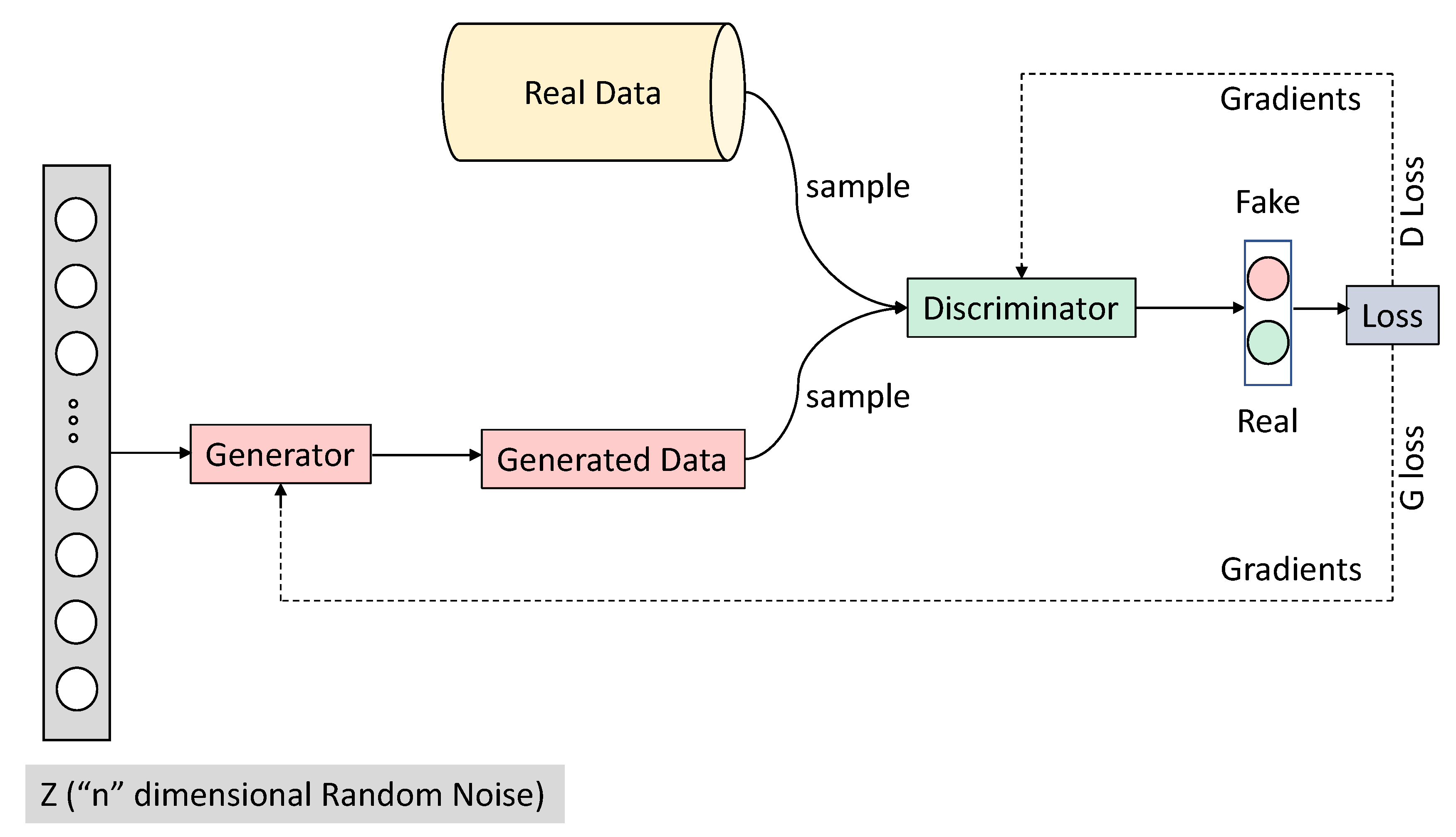
Ian Goodfellow and his colleagues introduced Generative Adversarial Networks (GANs) in 2014 [2], and Ian Goodfellow is often considered the inventor of GAN. GANs utilize two neural networks: a generator network and a discriminator network. Both are deep neural networks. A Generator network takes random noise as input to create samples (data) as realistic as possible to the original dataset, and a discriminator network distinguishes between real (actual data) and data (generated data) data, as shown in Figure 1.
GANs are a framework that learns to produce realistic objects that are difficult to differentiate from existing real objects, i.e., GANs capture the distribution of training data and generate new examples from the same distribution. GANs are versatile models that consist of two components, typically two distinct neural network models: a generator and a discriminator. The goal of the generator network is to produce plausible/fake examples. In contrast, the discriminator network’s goal is to differentiate between the real example from the training data and the fake example generated from the generator network.
Intuitively, one can think of the generator network as a forger that forges fake examples to try to look as realistic as possible and the discriminator network as an inspector that tries to tell which ones are real and which ones are fake. During training, the generator network gets better and better at producing artificial examples. In contrast, the discriminator learns to become a better investigator and properly distinguish the real and fake samples, i.e., it learns to model the probability of an example being real or fake. The probability of an example being real or fake from the discriminator is the one that helps the generator network to produce better examples/samples over time. This game’s equilibrium is where the generator produces realistic fake examples that look similar to actual examples from the training data. Simultaneously, the discriminator is left guessing at a 50% probability that the generated example is real or fake.
1.2. Deep Convolutional Generative Adversarial Network (DCGAN)
The DCGAN proposed by Radford et al. [3] is an extension of the original GAN [2], except that the discriminator network and generator network explicitly use convolutional and convolutional-transpose layers, respectively. In Section 3.1, we show the detailed architecture of the generator network, which maps the latent space vector () to dats space, and the presence of the batch normalization layers assist with healthy gradient flow during training [3]. Section 3.2 shows the detailed components of the discriminator network, which takes an image as input and outputs a scalar probability that the input image is real or fake. Instead of pooling to downsample, the discriminator network uses strided convolutional layers. It helps the network learn its own pooling feature, and, again, the presence of batch normalization layers and leaky ReLU activations facilitate healthy gradient flow during training [3].
2. Related Work
Data augmentation in the medical image domain is an active research field. In recent years, GANs have been employed by researchers to augment the datasets with various levels of success. Yi et al. [4] surveyed the same. We present a brief list of relevant works here. Chuquicusma et al. [5] proposed to use unsupervised learning with Deep Convolutional Generative Adversarial Networks (DC-GANs) to generate realistic lung nodule samples and evaluated the quality of generated nodules by presenting Visual Turing tests to two radiologists. Salehinejad et al. [6] demonstrated that augmenting the original imbalanced dataset with DCGAN generated images improved chest pathology classification performance. Madani et al. [7] utilized deep convolutional generative adversarial networks in a semi-supervised learning architecture for classification of cardiac abnormality in chest X-rays. Madani et al. [8] investigated DCGAN for generating chest X-ray images to augment the original dataset and trained a convolutional neural network to classify the images for cardiovascular abnormalities, which showed higher classification accuracy. Frid-Adar et al. [9] explored the use of GANs for data augmentation of liver lesion medical images. They showed that the GAN model used for synthetic data augmentation of liver lesion images improved the convolutional neural network (CNN) performance for liver lesion medical image classification. Bermudez et al. [10] used GANs for the unsupervised T1-weighted brain MRI synthesis by learning from 528 examples of 2D axial slices of brain MRI. Mondal et al. [11] explored generative adversarial networks for 3D multi-modal medical image segmentation and observed a significant performance improvement compared to the state-of-the-art segmentation networks. Lahari et al. [12] demonstrated the generative adversarial network framework for a structured prediction model for medical image segmentation and observed that the model outperformed fully supervised benchmark models by significant margins.
3. Materials and Methods
We used X-ray image data obtained by Kermany et al. [13] in the experiment. The dataset was already organized by Kermany et al. [13] into three folders (train, validation, and test). Each folder contained sub-folders for each image category (Normal/ Pneumonia).
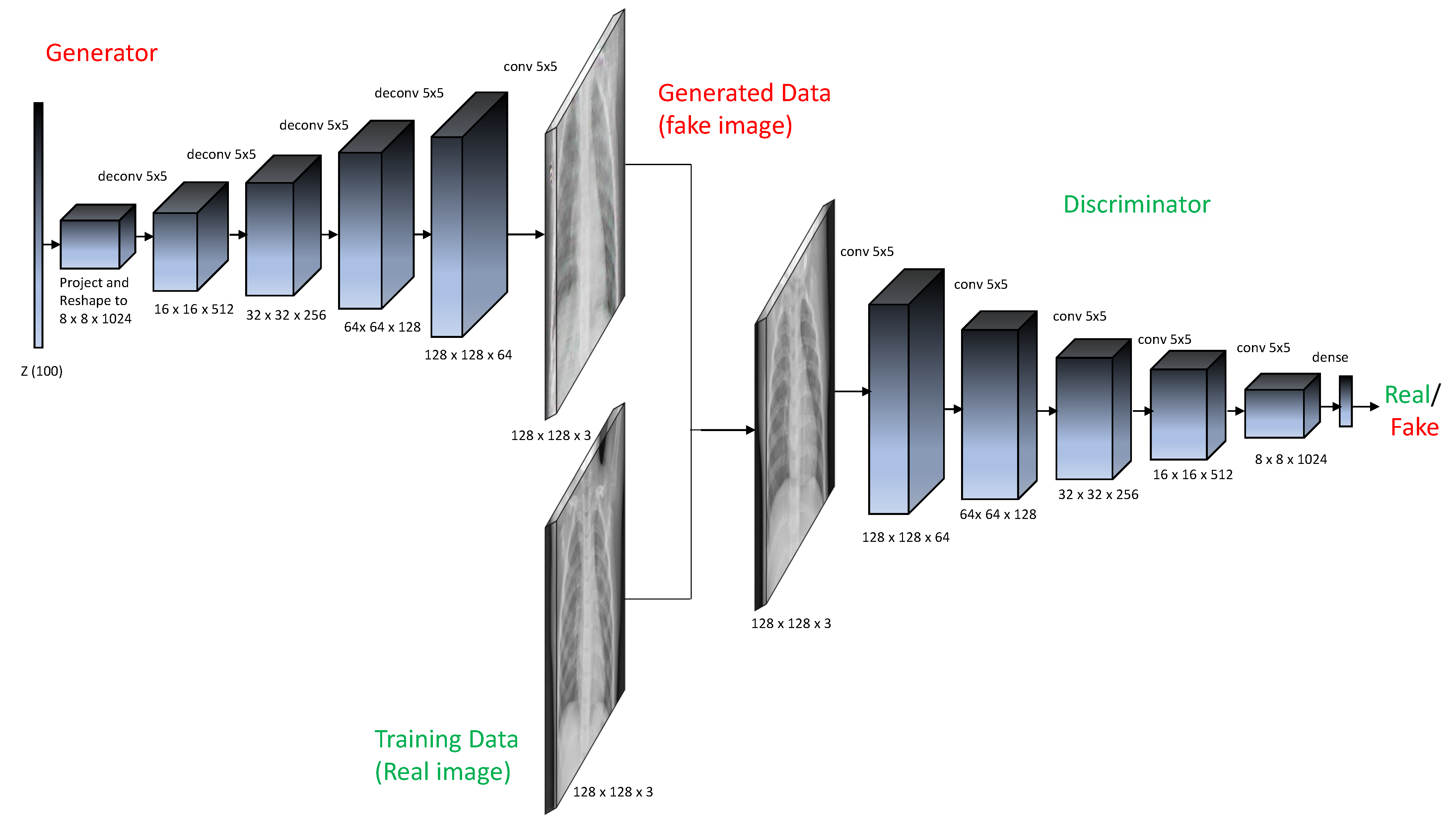
The train folder consists of 5216 X-ray images (1341 images labeled as Normal and 3875 images labeled as Pneumonia). There are 16 X-ray images in the validation folder, and 624 X-ray images in the test folder. It is evident that the data in the train folder are imbalanced, with the majority of the data labeled as Pneumonia, and training a deep neural network to classify the data among two categories will over-fit the data. This experiment augmented the Normal chest X-ray images by Deep Convolutional Generative Adversarial Networks (DCGAN). Figure 2 shows the architecture of the DCGAN.
First, because of GPU memory limitations, the images were resized to 128 × 128 pixels. Second, the images were scaled to a [−1,1] pixel value range to match the generator’s output as it uses the Tanh activation function. In this architecture, the generator network takes a 100 × 1 noise vector as input. There are then four convolutional-transpose layers with batch norm layers applied with the ReLU activation function interlaced in-between to scale to the appropriate 128 × 128 × 3 image size. A 128 × 128 × 3 image is taken as input by the discriminator network, followed by five strided convolution layers with batch norm layers and leaky ReLU as an activation function. A sigmoid activation function follows the last strided convolution block’s output to output whether the image is real (original data) or fake (generated data).
3.1. Generator Network
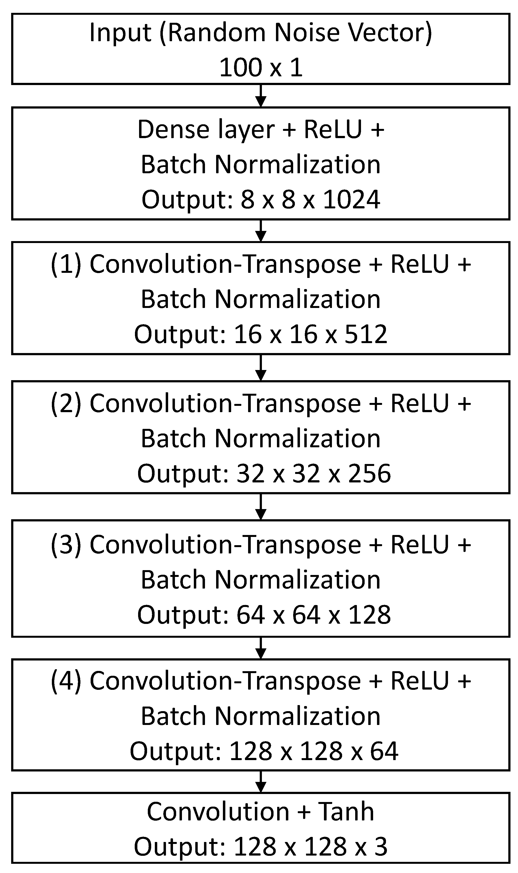
The detailed architecture of the generator network is shown in Figure 3. First, a generator network takes a 100 × 1 random noise vector as an input, which is fed to the dense layer to reshape the random noise vector to a representation of 8 × 8 × 1024. Second, to generate an image of size 128 × 128 × 3, the output from the dense layer is followed by a series of convolution-transpose layers to upsample the representation. Third, ReLU activation [14] is used, except for the output layer that uses Tanh activation, for all layers within the network. This enables the model to learn to saturation quickly and cover the training distribution’s color space [3]. Fourth, batch normalization [15] is used for all layers, except for the output layer, which normalizes the input to have zero mean and unit variance to stabilize the learning process. In this architecture, we use four convolution-transpose layers to upsample the representation of size 8 × 8 × 1024 to an image of size 128 × 128 × 3.
3.2. Discriminator Network
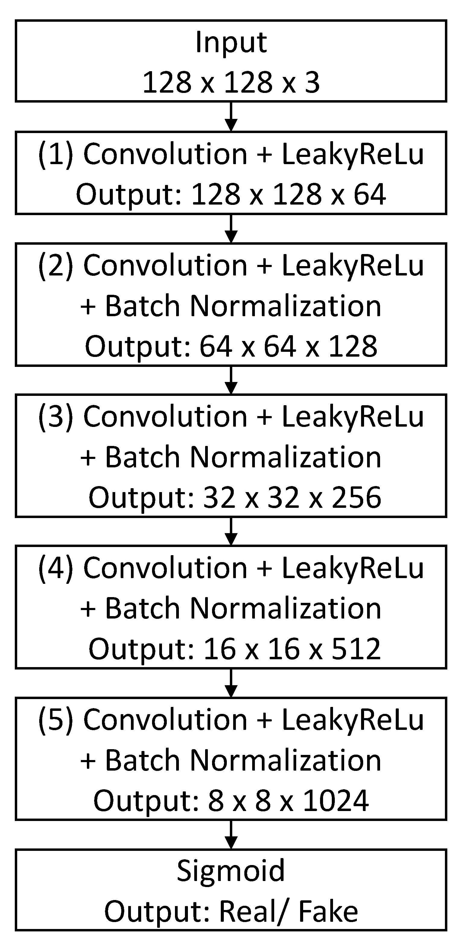
The goal of the discriminator network is to classify if the images are real or fake. The detailed architecture of the Discriminator Network is shown in Figure 4. The discriminator network takes images of size 128 × 128 × 3 as input, a combination of real images from the original dataset and the generated images from the generator network. In this network, the input image undergoes a series of convolutions, followed by a sigmoid activation function to output if the image is real or fake. As suggested by Radford et al. [3], each convolution block is followed by a LeakyReLU activation function [16] and Batch Normalization [15] is applied to all the layers in the network, except for the input layer.
3.3. GAN Objective Function
The objective of the GAN is to minimize the distance between the generated data probability distribution and real data probability distribution. In this study, we used the minimax loss introduced by Goodfellow et al. [2], which is given by Equation (1), where the generator network tries to minimize the loss function, and the discriminator network tries to maximize the same loss function. Thus, the GAN’s learning method is to simultaneously train discriminator and generator networks, which is a minmax game between the discriminator and the generator.
where is the expected value over all real instances, is the expected value over all the fake instances, is the random noise variable sampled from a standard normal distribution, is the generator function that maps to the data space, represents original data, and is the probability that came from the original data distribution rather than the generated data distribution [2].
The goal of is to estimate the distribution that the training data came from so it can generate fake samples from that estimated distribution [2]. The discriminator tries to maximize the likelihood that real images and fake images are correctly classified. Likewise, the generator tries to minimize . Theoretically, the solution to this minmax game is where = , such that the discriminator guesses randomly if the inputs are real images (training data) or fake images (generated data). However, GAN’s theory of convergence is still actively studied, and, to this extent, the models are not trained.
3.4. Loss Function
The discriminator network’s job is to classify the real images from the fake images, which is considered a binary classification problem. Thus, we use binary cross-entropy (BCE) as the loss function, which is given by Equation (2).
where M is the number of training examples in a mini-batch, is the target label for training example m (the real label is 1 and the fake label is 0), is the input for training example m, and is the model with neural network weights .
At the beginning of the equation, the summation sign indicates that we are summing over the variable M, i.e., taking the average cost of all the examples in the entire batch. The first term, , is the product of the true label times the log of the prediction, which is features parameterized by for the model that penalizes the probabilistic false negatives. In the perfect case, if the training model outputs 1, then the loss is = 0 and the training example is a real image. The same logic applies for the second term, , that penalizes the probabilistic false positives.
4. Results
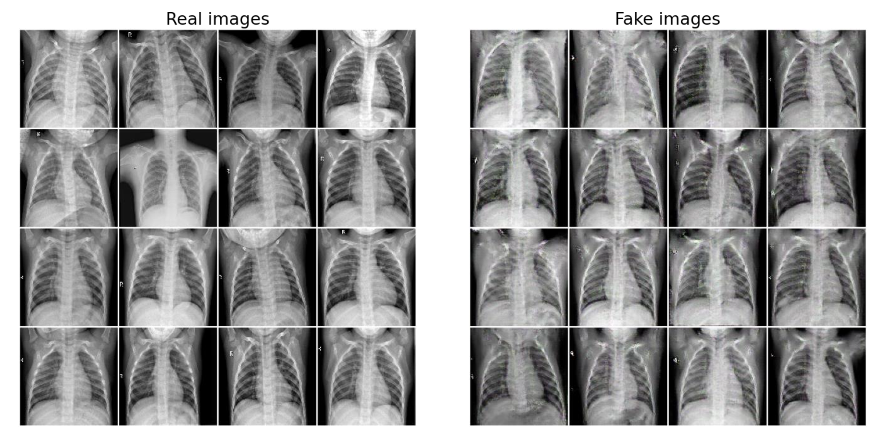
DCGAN training consists of two steps: (1) training the discriminator network; and (2) training the generator network. The objective is to train the discriminator to correctly classify the input image as real or fake and train the generator to produce better fake examples. First, the discriminator is trained with a batch of real examples to calculate . Second, the generator creates a batch of fake samples, and then the discriminator is trained with this batch of fake examples to calculate . We trained the DCGAN for 500 epochs, and the DCGAN was able to produce images that resembled chest X-ray images in about 50 epochs. Then, the quality of generated images further improved over 500 epochs.
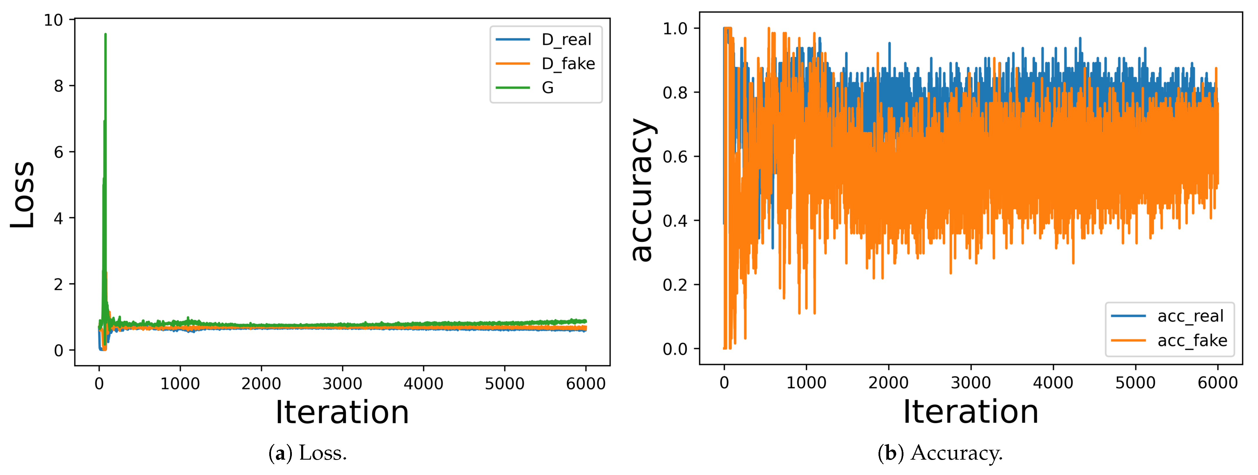
For comparison, we show a grid of real images (original data) and fake images (generated images) in Figure 5. During the GAN training, we simultaneously calculated the loss and accuracy of the discriminator and generator network. Referring to Section 3.3, a typical GAN model converges to a stable equilibrium when the discriminator loss is about 0.5, where the discriminator network is left to guess that the image is real or fake randomly. Simultaneously, the discriminator network’s accuracy on both real and fake images should be greater than 50%.
Figure 6 shows the loss and accuracy during the generator and discriminator training, where the generator loss and discriminator loss for both real and fake images is around 0.5, and the accuracy of the discriminator network is around 60–70%, indicating the GAN model converged to a stable equilibrium.
4.1. Evaluation
Deep learning models are usually trained with a loss function until neural network convergence. There is no loss function to train GAN generator models in order to objectively access the training progress and quality of the samples generated by the model from either the loss of the discriminator network or the loss of the generator network [17] because GANs are trained with two neural networks simultaneously to achieve a Nash equilibrium. In general, to access the quality of the generated images based on the GAN models’ performance, two techniques have been developed: (1) quantitative measures such as average log-likelihood, Inception Score (IS) [17], Fréchet Inception Distance (FID) [18], Maximum Mean Discrepancy (MMD) [19], etc.; and (2) qualitative measures such as nearest neighbours, rating and preference judgment, evaluating mode drop and mode collapse [20], etc. IS and FID are two widely accepted GAN evaluation measures [21]. In this work, we evaluate the DCGAN model using the FID measure.
4.1.1. FréChet Distance of Inception
The FID score is a measure used to evaluate the performance of GANs based on the quality of generated images. It captures the similarity of the generated images to the real images proposed by [18], which is an improvement on IS [17]. The FID score is calculated using the statistics of generated images to real images using the Fréchet distance also known as Wasserstein-2 distance, between the two multivariate Gaussians and is given by Equation (3),
where and are the feature-wise mean of real and generated images, respectively; and are the covariance matrix of real and generated images, respectively; is the trace which is the sum of the elements along the main diagonal of the square matrix; and and are the 2048-dimensional activations of the Inception-V3 pool3 layer for real images and generated images, respectively.
To calculate the Gaussian statistics (mean and covariance), the number of samples (real images and generated images, respectively) should be greater than the coding layer’s dimension, i.e., the samples should be greater than 2048 for the Inception-V3 pool 3 layer. Otherwise, there is no full rank of covariance matrix, resulting in NANs and complex numbers. Since we had very limited samples (fewer than 2048) in our training dataset, we could not take advantage of the Inception-V3 pool 3 layer, so we used the previous layer, a Pre-aux classifier, a 768-dimensional feature. We then calculated the (FID score using pyt [22], and the model achieved an FID score of 1.289 (lower scores correspond to better GAN performance).
4.1.2. Comparative Evaluation
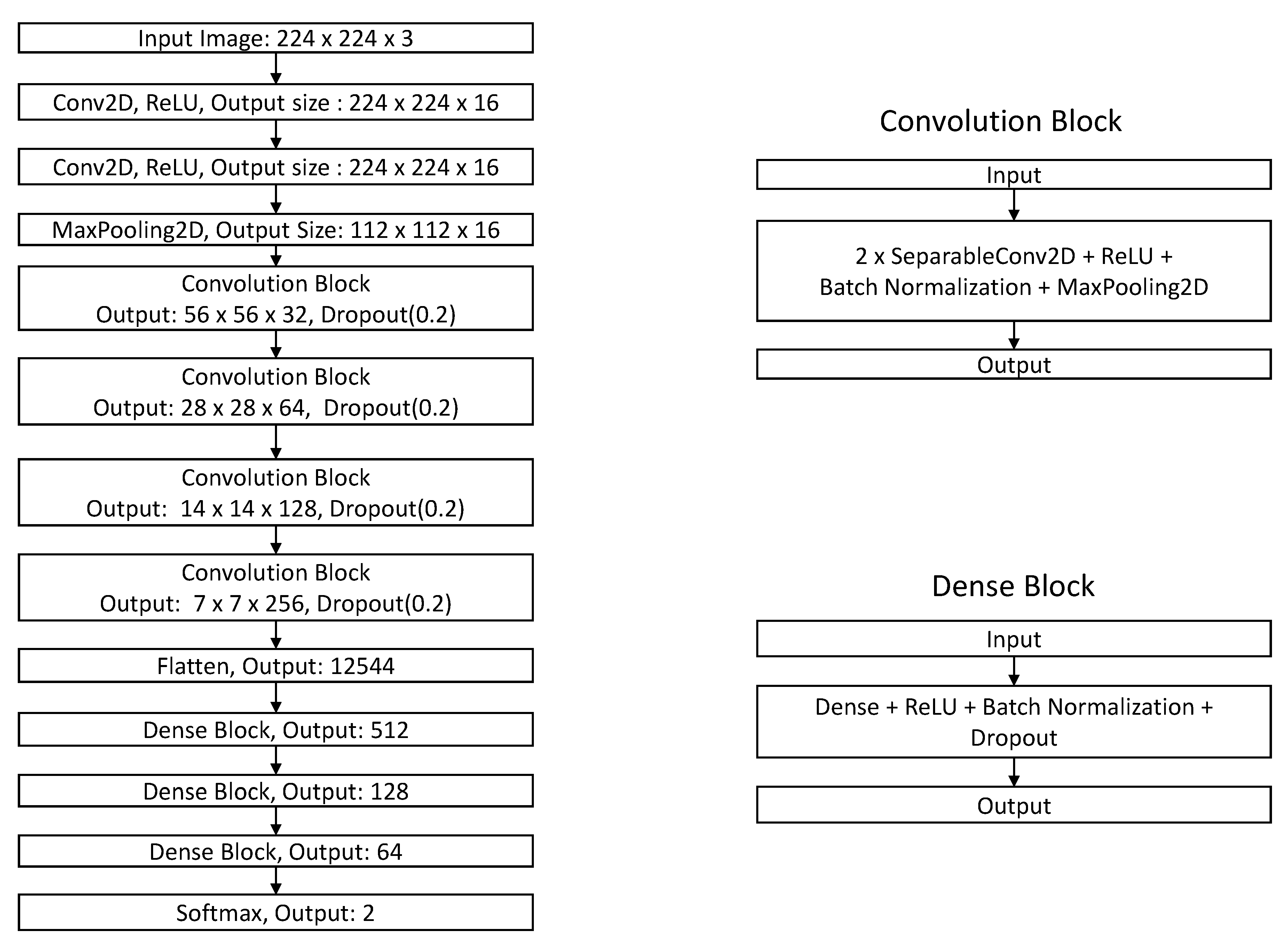
Further, we evaluated the comparative performance of DCGAN augmentation method. Improved data augmentation reduces over-fitting and results in better test accuracy. Thus, we trained a neural network classifier using GAN augmented dataset along with traditional augmented datasets with the architecture shown in Figure 7. The network takes an image of size 224 × 224 × 3 as an input, which is followed by two convolution layers to output a representation of size 224 × 224 × 16 and is subjected to the MaxPooling layer to output a representation of size 112 × 112 × 3. The output from the MaxPooling layer is subjected to four Convolutional blocks, where each convolution block consists of two separable convolution layers with ReLU activation, batch normalization, maxpooling, and dropout to output a representation of size 7 × 7 × 256. The 7 × 7 × 256 representation is flattened and then passed on to a series of dense blocks, which consists of a dense layer with batch normalization and dropout. The output from the last dense block is passed on to the softmax layer to output the probability of an image as Normal or Pneumonia. We used accuracy and receiver operating characteristics as evaluation metrics for model comparison.
Table 1 provides evidence that GAN based data augmentation results in improved accuracy of the classifier, which is also supported by the metrics of the confusion matrix, as shown in Table 2. While traditional data augmentation methods result in accuracy above 92%, GAN augmentation results in an accuracy of 95.5%. Contrast and brightness adjustment methods averaged 92% accuracy with varying levels of precision and recalls. Random crop and random flip methods have relatively better performance compared to adjustment methods, but still are inferior to GAN-based data augmentation.
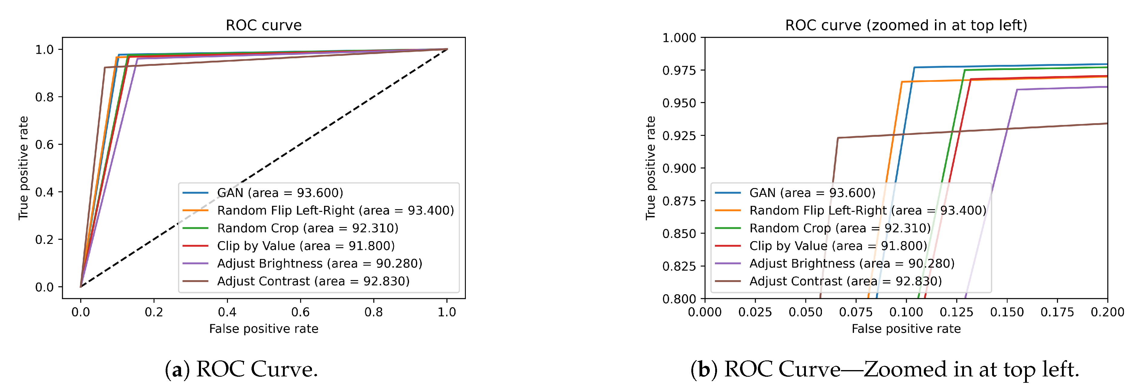
Table 1 presents the area under the ROC curve (AUC) for all data augmentation methods. The table shows that the GAN-based methods resulted in AUC of 93.6%, which is the best across all methods. While random flip method resulted in an AUC of 93.4%, all other methods have less than 93% AUC.
Figure 8 illustrates the ROC graphically. The graph confirms the superior performance of GAN based data augmentation over traditional augmentation methods. The comparative evaluation clearly demonstrates GAN methods superiority on both accuracy and ROC metrics.
Prior GAN based medical image augmentation research focused on evaluating image quality stand alone. Some works that evaluated the augmentation using ancillary tasks such as classification reported accuracy, precision, and recall in the range of 90%. Table 3 shows the details. While our task is different, the classification performance is better than these results. Kermany et al. [13] attempted classification of the current dataset using traditional augmentation methods and achieved an accuracy of 92.8%, sensitivity of 93.2%, and specificity of 90.1%. Our proposed model outperformed the classification metrics, achieving an accuracy of 95.5%, a precision of 96.2%, and a recall (sensitivity) of 97.7%.
5. Discussion
Usually, training deep learning models requires huge amounts of data. Data augmentation is a common technique used to increase the dataset sizes in data-limited situations, especially medical image datasets where there is limited access to the data due to the patients’ ethical/privacy concerns and high costs of obtaining the labeled data. In this study, we applied deep convolutional generative adversarial networks (DCGAN) to generate artificial chest X-ray images of the under-represented class (Normal) in the dataset that resembles the Normal chest X-ray images from the original dataset. Our results demonstrate that it is possible to generate plausible chest X-ray images using the DCGAN model with a small dataset of 1341 chest X-ray images. The evaluation of the model using FID achieved a score of 1.289, indicating that the synthetic images are close to the original images. Further, a neural classifier trained on DCGAN augmented datasets have superior performance compared to those generated using traditional methods. This higher performance indicates that the DCGAN generated synthetic images, compared to traditional methods, present additional information to the classifier, thereby reducing the over-fitting.
6. Conclusions
Researchers use data augmentation to increase the available sample size for training deep learning models. In computer vision tasks, this means generating synthetic images from the original dataset. While there are numerous methods to achieve this, imbalanced small sample sets create further challenges in the medical domain. The generation of a large number of high-resolution synthetic images can improve classifier performance significantly. This work demonstrates the utility of DCGAN methods for achieving the same. Hence, researchers working in the medical image analysis domain can use DCGAN for data augmentation and achieve better accuracy than traditional methods. In this study, we achieved high-quality synthetic image generation using the cross-entropy loss function. The future work can include the use of Wasserstein loss or Wasserstein loss with gradient penalty to replace the minimax loss to improve the quality of the generated images. In addition, combination methods such as stacking GAN samples with random cropping to further enhance the dataset can be attempted.
7. Forthcoming Research
- To test the visual quality of the generated X-ray images, we intend to supply the generated images to a clinician to label the images as either real or fake (generated).
Author Contributions
Conceptualization, S.K.V.; methodology, S.K.V.; software, S.K.V.; validation, S.K.V. and S.R.; formal analysis, S.K.V.; investigation, S.K.V.; resources, S.K.V.; data curation, S.K.V.; writing—original draft preparation, S.K.V.; writing—review and editing, S.K.V. and S.R.; visualization, S.K.V. and S.R.; and funding acquisition, S.R. All authors have read and agreed to the published version of the manuscript.
Funding
This research received no external funding.
Acknowledgments
We thank kermany et al. for making the datasets publicly accessible and we also thank Harrisburg University of Science and Technology for their support.
Conflicts of Interest
The authors declare no conflict of interest.
References
- Shorten, C.; Khoshgoftaar, T.M. A survey on image data augmentation for deep learning. J. Big Data 2019, 6, 60. [Google Scholar] [CrossRef]
- Goodfellow, I.; Pouget-Abadie, J.; Mirza, M.; Xu, B.; Warde-Farley, D.; Ozair, S.; Courville, A.; Bengio, Y. Generative adversarial nets. In Proceedings of the 27th International Conference on Neural Information Processing Systems, Montreal, QC, Canada, 8–13 December 2014; pp. 2672–2680. [Google Scholar]
- Radford, A.; Metz, L.; Chintala, S. Unsupervised representation learning with deep convolutional generative adversarial networks. arXiv 2015, arXiv:1511.06434. [Google Scholar]
- Yi, X.; Walia, E.; Babyn, P. Generative adversarial network in medical imaging: A review. Med. Image Anal. 2019, 58, 101552. [Google Scholar] [CrossRef] [PubMed] [Green Version]
- Chuquicusma, M.J.M.; Hussein, S.; Burt, J.; Bagci, U. How to Fool Radiologists with Generative Adversarial Networks? A Visual Turing Test for Lung Cancer Diagnosis. arXiv 2018, arXiv:1710.09762. [Google Scholar]
- Salehinejad, H.; Valaee, S.; Dowdell, T.; Colak, E.; Barfett, J. Generalization of Deep Neural Networks for Chest Pathology Classification in X-rays Using Generative Adversarial Networks. arXiv 2017, arXiv:1712.01636. [Google Scholar]
- Madani, A.; Moradi, M.; Karargyris, A.; Syeda-Mahmood, T. Semi-supervised learning with generative adversarial networks for chest X-ray classification with ability of data domain adaptation. In Proceedings of the 2018 IEEE 15th International Symposium on Biomedical Imaging (ISBI 2018), Washington, DC, USA, 4–7 April 2018; pp. 1038–1042. [Google Scholar]
- Madani, A.; Moradi, M.; Karargyris, A.; Syeda-Mahmood, T. Chest X-ray generation and data augmentation for cardiovascular abnormality classification. In Proceedings of the Medical Imaging 2018, Image Processing, Houston, TX, USA, 10–15 February 2018; Angelini, E.D., Landman, B.A., Eds.; International Society for Optics and Photonics, SPIE: Bellingham, WA, USA, 2018; Volume 10574, pp. 415–420. [Google Scholar] [CrossRef]
- Frid-Adar, M.; Diamant, I.; Klang, E.; Amitai, M.; Goldberger, J.; Greenspan, H. GAN-based synthetic medical image augmentation for increased CNN performance in liver lesion classification. Neurocomputing 2018, 321, 321–331. [Google Scholar] [CrossRef] [Green Version]
- Bermudez, C.; Plassard, A.J.; Davis, L.T.; Newton, A.T.; Resnick, S.M.; Landman, B.A. Learning Implicit Brain MRI Manifolds with Deep Learning. arXiv 2018, arXiv:1801.01847. [Google Scholar]
- Mondal, A.K.; Dolz, J.; Desrosiers, C. Few-shot 3D Multi-modal Medical Image Segmentation using Generative Adversarial Learning. arXiv 2018, arXiv:1810.12241. [Google Scholar]
- Lahiri, A.; Jain, V.; Mondal, A.; Biswas, P.K. Retinal Vessel Segmentation under Extreme Low Annotation: A Generative Adversarial Network Approach. arXiv 2018, arXiv:1809.01348. [Google Scholar]
- Kermany, D.S.; Goldbaum, M.; Cai, W.; Valentim, C.C.; Liang, H.; Baxter, S.L.; McKeown, A.; Yang, G.; Wu, X.; Yan, F.; et al. Identifying medical diagnoses and treatable diseases by image-based deep learning. Cell 2018, 172, 1122–1131. [Google Scholar] [CrossRef] [PubMed]
- Nair, V.; Hinton, G.E. Rectified linear units improve restricted boltzmann machines. In Proceedings of the 27th International Conference on International Conference on Machine Learning, Madison, WI, USA, 21–24 June 2010. [Google Scholar]
- Ioffe, S.; Szegedy, C. Batch normalization: Accelerating deep network training by reducing internal covariate shift. arXiv 2015, arXiv:1502.03167. [Google Scholar]
- Xu, B.; Wang, N.; Chen, T.; Li, M. Empirical evaluation of rectified activations in convolutional network. arXiv 2015, arXiv:1505.00853. [Google Scholar]
- Salimans, T.; Goodfellow, I.; Zaremba, W.; Cheung, V.; Radford, A.; Chen, X. Improved Techniques for Training GANs. arXiv 2016, arXiv:1606.03498. [Google Scholar]
- Heusel, M.; Ramsauer, H.; Unterthiner, T.; Nessler, B.; Hochreiter, S. GANs Trained by a Two Time-Scale Update Rule Converge to a Local Nash Equilibrium. arXiv 2017, arXiv:1706.08500. [Google Scholar]
- Fortet, R.; Mourier, E. Convergence of the empirical distribution towards the theoretical distribution. Sci. Ann. Ecole Norm. Supérieure 1953, 70, 267–285. [Google Scholar] [CrossRef]
- Srivastava, A.; Valkov, L.; Russell, C.; Gutmann, M.U.; Sutton, C. VEEGAN: Reducing Mode Collapse in GANs using Implicit Variational Learning. arXiv 2017, arXiv:1705.07761. [Google Scholar]
- Borji, A. Pros and Cons of GAN Evaluation Measures. arXiv 2018, arXiv:1802.03446. [Google Scholar] [CrossRef] [Green Version]
- pytorch-fid · PyPI. Available online: https://pypi.org/project/pytorch-fid/ (accessed on 9 January 2020).
- Tang, Y.; Cai, J.; Lu, L.; Harrison, A.P.; Yan, K.; Xiao, J.; Yang, L.; Summers, R.M. CT image enhancement using stacked generative adversarial networks and transfer learning for lesion segmentation improvement. In Proceedings of the International Workshop on Machine Learning in Medical Imaging, Granada, Spain, 16 September 2018; Springer: Berlin/Heidelberg, Germany, 2018; pp. 46–54. [Google Scholar]
Figure 1.
Generative Adversarial Network Architecture.

Figure 2.
Deep Convolutional Generative Adversarial Network Architecture.

Figure 3.
Generator Network Architecture.

Figure 4.
Discriminator Network Architecture.

Figure 5.
Images from the original dataset (real) and images generated by the generator of DCGAN (fake).
Figure 5.
Images from the original dataset (real) and images generated by the generator of DCGAN (fake).

Figure 6.
Generator and discriminator network loss and accuracy during training.

Figure 7.
Convolutional Neural Network Architecture.

Figure 8.
Receiver operating characteristics curve.


Table 1.
Classification performance metrics.
| Model/ Method | Accuracy | Precission | Recall | F1 Score | AUC | FPR | TPR |
|---|---|---|---|---|---|---|---|
| Randomflip-leftright | 94.9 | 96.39 | 96.6 | 96.5 | 93.4 | 0.09 | 0.97 |
| RandomCrop | 94.71 | 95.31 | 97.54 | 96.42 | 92.31 | 0.13 | 0.98 |
| ClipByValue | 94.11 | 95.17 | 96.84 | 96 | 91.8 | 0.13 | 0.97 |
| AdjustBrightness | 92.91 | 94.37 | 96.02 | 95.18 | 90.28 | 0.16 | 0.96 |
| AdjustContrast | 92.58 | 97.41 | 92.29 | 94.77 | 92.83 | 0.07 | 0.92 |
| GAN | 95.5 | 96.2 | 97.7 | 97 | 93.6 | 0.1 | 0.98 |
Table 2.
Confusion matrix.
| Model/ Method | True Negative | False Positive | False Negative | True Positive |
|---|---|---|---|---|
| Randomflip-leftright | 286 | 31 | 29 | 826 |
| RandomCrop | 276 | 41 | 21 | 834 |
| ClipByValue | 275 | 42 | 27 | 828 |
| AdjustBrightness | 268 | 49 | 34 | 821 |
| AdjustContrast | 296 | 21 | 66 | 789 |
| GAN | 284 | 33 | 20 | 835 |
Publisher’s Note: MDPI stays neutral with regard to jurisdictional claims in published maps and institutional affiliations. |
© 2020 by the authors. Licensee MDPI, Basel, Switzerland. This article is an open access article distributed under the terms and conditions of the Creative Commons Attribution (CC BY) license (http://creativecommons.org/licenses/by/4.0/).
Share and Cite
MDPI and ACS Style
Kora Venu, S.; Ravula, S. Evaluation of Deep Convolutional Generative Adversarial Networks for Data Augmentation of Chest X-ray Images. Future Internet 2021, 13, 8. https://0-doi-org.brum.beds.ac.uk/10.3390/fi13010008
AMA Style
Kora Venu S, Ravula S. Evaluation of Deep Convolutional Generative Adversarial Networks for Data Augmentation of Chest X-ray Images. Future Internet. 2021; 13(1):8. https://0-doi-org.brum.beds.ac.uk/10.3390/fi13010008
Chicago/Turabian StyleKora Venu, Sagar, and Sridhar Ravula. 2021. "Evaluation of Deep Convolutional Generative Adversarial Networks for Data Augmentation of Chest X-ray Images" Future Internet 13, no. 1: 8. https://0-doi-org.brum.beds.ac.uk/10.3390/fi13010008
Note that from the first issue of 2016, this journal uses article numbers instead of page numbers. See further details here.