
Underwater Target Recognition Based on Multi-Decision LOFAR Spectrum Enhancement: A Deep-Learning Approach


National Key Laboratory of Science and Technology on Communications, University of Electronic Science and Technology of China, Chengdu 610054, China
*
Author to whom correspondence should be addressed.
Future Internet 2021, 13(10), 265; https://0-doi-org.brum.beds.ac.uk/10.3390/fi13100265
Submission received: 10 September 2021
/
Revised: 2 October 2021
/
Accepted: 5 October 2021
/
Published: 13 October 2021
(This article belongs to the Special Issue Machine Learning for Wireless Communications)
Abstract
:Underwater target recognition is an important supporting technology for the development of marine resources, which is mainly limited by the purity of feature extraction and the universality of recognition schemes. The low-frequency analysis and recording (LOFAR) spectrum is one of the key features of the underwater target, which can be used for feature extraction. However, the complex underwater environment noise and the extremely low signal-to-noise ratio of the target signal lead to breakpoints in the LOFAR spectrum, which seriously hinders the underwater target recognition. To overcome this issue and to further improve the recognition performance, we adopted a deep-learning approach for underwater target recognition, and a novel LOFAR spectrum enhancement (LSE)-based underwater target-recognition scheme was proposed, which consists of preprocessing, offline training, and online testing. In preprocessing, we specifically design a LOFAR spectrum enhancement based on multi-step decision algorithm to recover the breakpoints in LOFAR spectrum. In offline training, the enhanced LOFAR spectrum is adopted as the input of convolutional neural network (CNN) and a LOFAR-based CNN (LOFAR-CNN) for online recognition is developed. Taking advantage of the powerful capability of CNN in feature extraction, the recognition accuracy can be further improved by the proposed LOFAR-CNN. Finally, extensive simulation results demonstrate that the LOFAR-CNN network can achieve a recognition accuracy of 95.22%, which outperforms the state-of-the-art methods.
1. Introduction
The ocean contains rich mineral resources, marine living resources and chemical resources. Its huge economic value has attracted the attention of almost all coastal countries in the world. Therefore, ocean development such as seabed exploration, oil platform monitoring, and economic fish detection is of great significance. The ability to accurately determine whether an underwater target is an ordinary aquatic fish or a dangerous obstacle with the help of underwater acoustic target-recognition technology is extremely critical to the safety of shipping vessels. Deep Learning (DL) is a discipline that specializes in how computers simulate or implement human learning behaviors to acquire new knowledge or skills, and reorganize the existing knowledge structure to continuously improve its own performance [1,2,3]. It is found that it also has a good performance in the field of communications. Underwater target recognition based on DL is a new method to realize underwater target recognition based on existing recognition methods. Using this method, it can automatically extract features from the original signal, compress feature vectors, fit the target map, reduce the impact of noise, avoid feature loss during manual extraction, improve generalization capabilities, and constantly improve the efficiency and accuracy of identification during the model process.
The application of deep learning in the field of underwater target recognition mainly involves three aspects. The first is the field of underwater recognition. Due to many reasons such as confidentiality and security, the collection and production of data sets are difficult. Therefore, researchers will use as many existing samples as possible, such as using Generative Adversarial Networks (GAN) to achieve sample expansion to meet the needs of deep learning with large data volumes. The second is the orthodox field of deep learning, such as computer vision and natural language recognition. Researchers start from optimizing and designing complex deep neural network structures, and only rely on neural networks to complete feature extraction. The third is the data preprocessing stage before inputting the neural network. In view of the serious pollution of the collected data by environmental noise, researchers perform denoising and spectral transformation on audio samples, or perform image denoising on sonar images. Its purpose is to make the sample features as obvious as possible through feature engineering, which is more conducive to the needs of deep neural network feature extraction.
In this paper, we are interested in underwater target-recognition methods based on deep learning. The Low-frequency analysis and recording (LOFAR) spectrum is widely used in the field of passive sonar ship target recognition due to its significant sound source information and relatively high signal-to-noise ratio. It transforms the signal from the time domain to the time-frequency domain. Sonars usually observe the line spectrum in the LOFAR spectrum to determine whether the target exists, and perform tracking and recognition. This type of method is mainly realized by extracting features and training classifiers. Unfortunately, because the data are always contaminated by environmental noise, breakpoints are introduced in the LOFAR spectrum, which reduces the performance of signal processing. To overcome this problem and further improve the performance of underwater target recognition, we use deep-learning methods for underwater target recognition, and propose an underwater target-recognition scheme based on LOFAR spectral enhancement (LSE). This solution can restore the breakpoints in the LOFAR spectrum and combine with Convolutional Neural Network (CNN) for online recognition, which reduces the impact of environmental noise and significantly improves the target recognition rate of existing algorithms.
1.1. Contributions
The main contributions of this paper are summarized as follows:
- (1)
- In contrast to the traditional algorithm, we use the decomposition algorithm based on resonance signal to preprocess the signal. Based on the multi-step decision algorithm with the line spectrum characteristic cost function [4], this paper proposes the specific calculation method of double threshold. In the purpose, this algorithm not only retains the continuous spectrum information in the original LOFAR spectrum, but also merges the extracted line spectrum with the original LOFAR spectrum. Finally, the breakpoint completion of the LOFAR spectrum is realized.
- (2)
- To further improve the recognition rate of underwater targets, we adopt the enhanced LOFAR spectrum as the input of CNN and develop a LOFAR-based CNN (LOFAR-CNN) for online recognition. Taking advantage of the powerful capability of CNN in feature extraction, the proposed LOFAR-CNN can further improve the recognition accuracy.
- (3)
- Simulation results demonstrate that when testing on the ShipsEar database [5], our proposed LOFAR-CNN method can achieve a recognition accuracy of 95.22% which outperforms the state-of-the-art methods.
1.2. Related Works
Recently, CNN has proven its powerful capability in many fields, such as computer vision, nature language processing, and wireless physical layer [6,7,8]. Convolutional neural networks are deep feedforward neural networks that include operations such as convolution calculations, pooled sampling, and nonlinear activation [4,9,10]. Compared with the traditional feedforward neural networks such as MLP, three strategies in CNN make use of the spatial correlation of data which include weight sharing, local receptive field and down sampling. They reduce the risk of over fitting, the defect of gradient disappearance the complexity and parameter size of the network. However, they improve the generalization ability of the network. CNN was first proposed by LeCun [11] in 1990 and applied to the handwritten character detection system. In 2014, Szegedy [12] proposed GoogleLeNet which introduced the inception module. Receptive fields of different sizes enhanced the adaptability of the network to scale. The improved version [13,14] greatly reduces the parameter amount to enhance the nonlinearity of the network and speed up the calculation. The residual network was proposed by Kaiming. He [15] in 2015 adopted the idea of Shortcut Connection (SC) to solve the problem of network degradation. After full investigation and experimental verification, CNN is very suitable for underwater target recognition.
In addition, many effective and efficient DL-based schemes have been proposed for underwater target recognition. For example, Refs. [16,17] focused on underwater target recognition which have sufficient training samples. In the first step, the original audio was converted into LOFAR spectrum, and then GAN was used for sample expansion. In the second step, a 15% performance improvement could be obtained using convolutional neural networks (CNNs) for feature learning and classification when the number of samples was more sufficient. Ref. [18] combined competitive learning with deep belief network (DBN) and proposed a deep competitive network that used unlabeled samples to solve small number of samples in acoustic target recognition. This method could achieve a classification accuracy of 90.89%. To address the negative impact of redundant features on recognition accuracy and efficiency, the authors in [19] proposed a compressed deep competition network which combined network pruning with training quantization and other technologies and could achieve a classification accuracy of 89.1%. Refs. [20,21] proposed a new time-frequency feature extraction method by jointly exploiting the resonance-based sparse signal decomposition (RSSD) algorithm, the phase space reconstruction (PSR), the time-frequency distribution (TFD), and the manifold learning. At the same time, a one-dimensional convolutional auto-encoder-decoder model was used to further extract and separate features from high-resonance components, which finally completed the recognition task and achieves a recognition accuracy of 93.28%. In addition, Refs. [22,23,24] all used convolutional neural networks for feature extraction, but the application scenarios and the classifiers were different. Ref. [22] proposed an automatic target-recognition method of unmanned underwater vehicle (UUV), which adopted CNN to extract features from sonar images and used support vector machine (SVM) classifier to complete the classification. Ref. [23] aimed to study different types of marine mammals. It also used the CNN+SVM structure to complete the feature extraction and classification recognition task. It compared the two classification and multi-class task scenarios. Ref. [24] adopted the civil ship data set and exploited the framework structure of CNN+ELM (extreme learning machine) as the underwater target classifier, which improved the recognition accuracy. We can see that with the in-depth research of scholars, the recognition rate of underwater targets based on deep learning has gradually increased.
1.3. Organization
The rest of this article is organized as follows. The second section introduces the model of the system. The third section introduces the deep-learning underwater target signal recognition framework based on multi-step decision LOFAR line spectrum enhancement. The fourth section is the experimental verification and simulation results of our proposed algorithm framework. The fifth section is the summary of the article.
Some notations in this paper are shown in the following. and respectively represent the L2 norm and L1 norm. is short-time Fourier transform. Term is the statistical expectation. represents the variable value when the objective function is minimized.
2. System Model
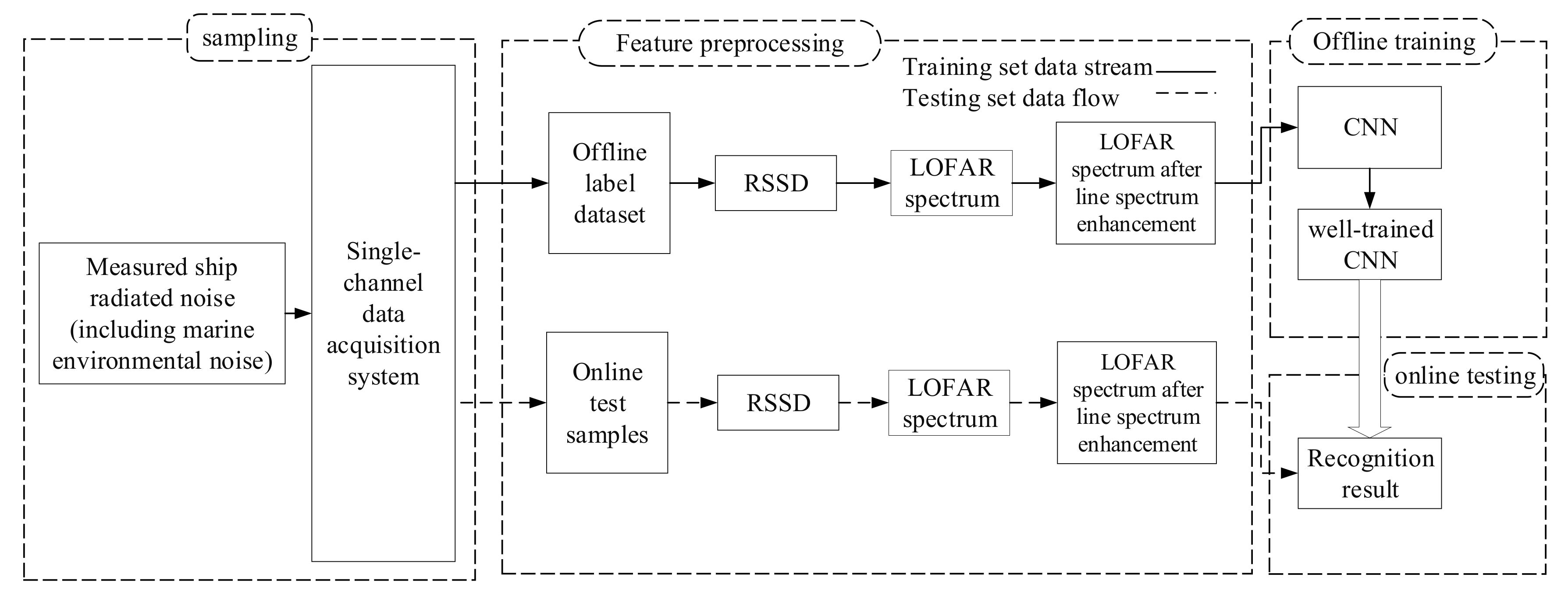
In this paper, we consider a deep-learning underwater target-recognition framework based on multi-step decision LOFAR line spectrum enhancement which is shown in Figure 1. It is divided into four modules: sampling, feature preprocessing, offline training and online testing.
2.1. Signal Decomposition Algorithm Based on Resonance
In traditional signal processing, Fourier transform is usually used to analyze in the frequency domain or time-frequency domain, but these methods are only valid for periodic stationary signals [25]. However, due to the generation mechanism of ship radiated noise and the complex channel conditions in the marine environment, the ship radiated noise collected by hydrophones is usually the mixture of oscillating signals and transient non-oscillating signals [20]. The harmonic component (or oscillation component) of the ship’s radiated noise plays an important role in the identification of underwater targets. Therefore, a signal decomposition algorithm based on resonance that effectively responds to nonlinear signals is used to preprocess the signal. Based on the oscillation characteristics rather than the frequency or scale, the method can obtain a signal composed of multiple simultaneous and continuous oscillations (high-resonance component). To some extent, it weakens the transient non-oscillation signal of uncertain duration (low-resonance component) and gaussian white noise (residual component) which is conducive to feature extraction.
The RSSD algorithm regards resonance as the basis for signal decomposition [26], and the Q factor quantifies the degree of signal resonance. Specifically, high-resonance signals exhibit a higher degree of frequency aggregation in the time domain, more simultaneous oscillating waveforms with a larger Q factor. Low-resonance signals appear non-oscillating and indefinite transient signal with a smaller Q factor. Therefore, the basic theory of the RSSD algorithm is that using two different wavelet basis functions (corresponding to Q factors of different sizes), we can find a sparse representation of a complex signal and reconstruct the signal.
The algorithm mentioned in this section is divided into adjustable Q-Factor Wavelet Transform (TQWT) [27] and Morphological Component Analysis (MCA) [28]. Its algorithm framework is shown in Figure 2.
2.1.1. Morphological Component Analysis
Morphological component analysis is usually used to decompose signals with different morphological characteristics [29]. The ship radiated noise with oscillating and non-oscillating component has different morphological characteristics. So, the MCA algorithm can be used to separate and extract the ship radiated noise to construct the optimal sparse representation for its high-resonance and low-resonance component.
Considering the discrete ship radiated noise sequence, the signal can be sparsely expressed as:
where , are the wavelet coefficients corresponding to the high resonant component and the low resonant component . , are wavelet basis functions corresponding to , . n represents the residual components of the signal which removes first two.
The purpose of MCA is to obtain an optimal representation , of the high-resonance component and low-resonance component of the signal. This problem can be solved by minimizing the following objective function:
Here, and represent the number of decomposition layers of and . and are the wavelet coefficients of the high-resonance component and the low-resonance component of the jth layer, respectively. , are the normalized coefficients of , and their values are related to energy of , :
where , , are the proportionality coefficient of the energy distribution of the high-resonance component and the low-resonance component. are selected to balance the energy distribution of the two components.
Through decomposition of the Augmented Lagrangian Shrinkage Algorithm (SALSA) [26], the optimal wavelet coefficients can be obtained by solving the optimization problem of the formula. Therefore, the optimal expressions for the high-resonance component and the low-resonance component obtained by the MCA algorithm are:
In summary, the purpose of the RSSD algorithm is to construct the optimal sparse representation of the high and low-resonance components of the ship radiated noise. The specific steps can be expressed as follows:
- (1)
- Select the appropriate filter scaling factor , according to the waveform characteristics of the signal. Then calculate the parameters , , corresponding to the high-resonance component, and the parameters , , corresponding to the low-resonance component. At last, construct the corresponding wavelet basis function , .
- (2)
- Reasonably set the weighting coefficient , of the L1 norm of the wavelet coefficients of each layer. Obtain the optimal wavelet coefficient , by minimizing the objective function through the SALSA algorithm.
- (3)
- Reconstruct the optimal sparse representation , of high-resonance components and low-resonance components.
2.1.2. Adjustable Q-Factor Wavelet Transform
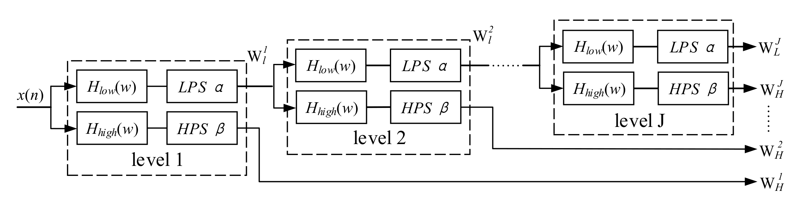
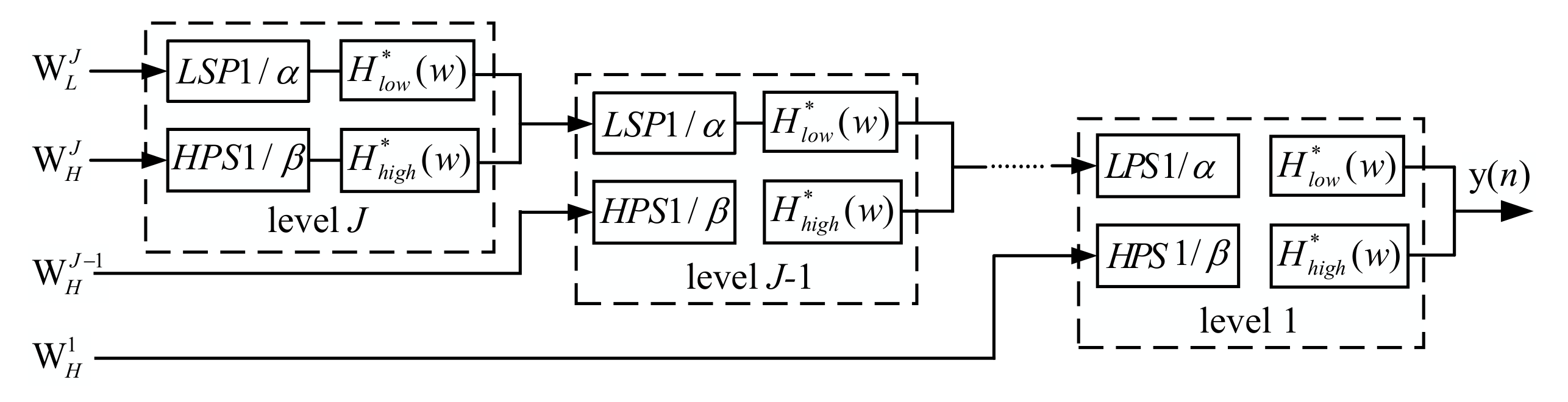
TQWT is a discrete wavelet transform that can flexibly adjust the constant Q factor according to the resonance of the processed signal, which has an overcomplete basis and can be perfectly reconstructed [30]. This section uses the TQWT toolbox to complete simulation experiments and signal processing. The implementation framework consists of two filter banks which are analysis filter bank and integrated filter bank. They are shown in Figure 3 and Figure 4. A filter bank refers to a group of filters. They have a common input, or a common output. The analysis filter bank has a common input to obtain multiple subband signals. In contrast, the integrated filter has a common output, combining multiple subband signals into a single signal to restore the original analyzed signal.
The analysis filter bank of each layer is composed of high-pass filter , low-pass filter , and the corresponding scaling process, which are defined as follows:
is the Daubechies filter with second-order disappearing moment [27]. , are the scaling factors after the signal passes through the low-pass and high-pass filters, respectively. The scaling process of low-pass and high-pass are defined as:
The Q factor quantifies the degree of signal resonance, and its definition is , where represents the center frequency of the signal and represents the bandwidth.
If the sampling frequency of the original input signal is , then the center frequency , the filter bank level j and , [31] can be expressed as:
Similarly, bandwidth can be expressed as:
Therefore, the Q factor is derived as:
After the original signal passes through the filter bank, the output of the low-pass channel is iteratively inputted to the deeper level filter bank until the preset level J. At the same time, the wavelet basis functions , are constructed by selecting the oversampling rate r. The deepest level and the oversampling rate r are defined as follows:
In summary, in the TQWT algorithm, Q, r, J can be calculated by selecting , , and , selection is only determined by the inherent oscillation characteristics of the signal. Therefore, it can flexibly select , according to the specific requirements of Q, r, J. For the input signal of ship radiated noise, we need to set , , to extract its high-resonance information and set , , to extract its low-resonance information.
3. LOFAR Spectral Line Enhancement Based on Multi-Step Decision
The line spectrum has been widely used in the field of passive sonar ship target recognition because of its significant sound source information and relatively high signal-to-noise ratio. The Low-Frequency Analysis Representation (LOFAR) spectrum transforms the signal received by the passive sonar from time domain to time-frequency domain using the short-time Fourier transform (STFT), which can reflect the signal in the two dimensions of time domain and frequency domain. Scientists observe the line spectrum in the LOFAR spectrum to determine the presence or absence of the target, and perform tracking and recognition [9]. Because there is more demand of the stealth technology of the ship and the radiated noise of the ship’s target is greatly reduced, the signal-to-noise ratio of the ship radiated noise received by the hydrophone array is also decreasing. The line spectrum components become more difficult to identify. There are many research results on automatic detection and extraction of line spectrum under low signal-to-noise ratio.
In this paper, we study from the multi-step decision algorithm based on the line spectrum feature cost function proposed by Di Martino [32]. Then we propose a specific calculation method of double threshold, and retain the continuous spectrum information in the original LOFAR spectrum. At last, we combine the original LOFAR spectrum with the extracted line spectrum, and complete the recognition and detection of underwater target by making full use of the advantages of deep neural network feature extraction.
3.1. Structure LOFAR Spectrum
The LOFAR spectrum is calculated by short-time Fourier transform (STFT). Unlike the traditional Fourier transform, which requires signal stability, STFT is suitable for non-stationary signals. It takes advantage of the short-term stationary characteristics of the signal. After windowing and framing the signal, the Fourier transform is performed to obtain the signal at time-frequency. Then it is more accurately characterize the distribution of signal frequency components and time nodes. The calculation formula is as follows:
where is short-time Fourier transform, is the signal to be transformed and is the window function (truncating function). The process of calculating the LOFAR spectrum can be compared with the “LOFAR Spectrum” in the Feature Processing stage in Figure 1. The specific calculation steps are as follows:
- (1)
- Framing and windowing. The sound signal is unstable globally, but can be regarded as stable locally. In the subsequent speech processing, a stable signal needs to be input. Therefore, it is necessary to frame the entire speech signal, i.e., to divide it into multiple segments. We divide the sampling sequence of the signal into K frames and each frame contains N sampling points. The larger the N and K, the larger the amount of data, and the closer the final result is to the true value. Due to the correlation between the frames, there are usually some points overlap between the two frames. Framing is equivalent to truncating the signal, which will cause distortion of its spectrum and leakage of its spectral energy. To reduce spectral energy leakage, different truncation functions which are called window function can be used to truncate the signal. The practical application window functions include Hamming window, rectangular window and Hanning window, etc.
- (2)
- Normalization and decentralization. The signal of each frame needs to be normalized and decentralized, which can be calculated by the following formula:Here, is the normalization of , which makes the power of the signal uniform in time. is the decentralization of , which makes the mean of the samples zero.
- (3)
- Perform Fourier transform on each frame signal and arrange the transformed spectrum in the time domain to obtain the LOFAR spectrum.
3.2. Analysis and Construction of Line Spectrum Cost Function
The definition of the line spectrum feature cost function is as follows:
where represents a summation path along the time axis in the observation window of the LOFAR graph, and the length of the path is N. characterize the amplitude characteristics of the line spectrum, is the frequency continuity of the line spectrum, and is the trajectory continuity of the line spectrum, and are weighting coefficients. The definitions of , , and are as follows:
Each pixel on the summing path is , which means a point on the i line of the time axis. characterizes the amplitude of the point . characterizes the frequency gradient at two points in the path, which is defined as follows:
where represents the frequency of the point . characterizes the breakpoint identification, which is defined as follows:
If the amplitude of the point is less than , it is regarded as a breakpoint and recorded as 1, otherwise it is recorded as 0. Regarding the calculation of the threshold , the original algorithm is mostly set by empirical values, and a new calculation method is proposed as follows:
where represents the marine environmental noise. The sampling sequence of the interference noise in the marine environment is subjected to STFT transformation which can obtain the LOFAR spectrum. At the same time, the instantaneous power of each time-frequency point is calculated. M, N represent the points of frequency domain and time domain of LOFAR spectrum. The power of all time and frequency points is summed and averaged to obtain the average power. Take a square to obtain the average amplitude of the LOFAR spectrum of marine environment interference noise, which is the threshold for determining whether the point is a breakpoint.
It can be analyzed from the cost function: the problem of line spectrum detection is transformed into the problem of finding the optimal path and minimizing the cost function about the path .
3.3. Sliding Window Line Spectrum Extraction Algorithm Based on Multi-Step Decision
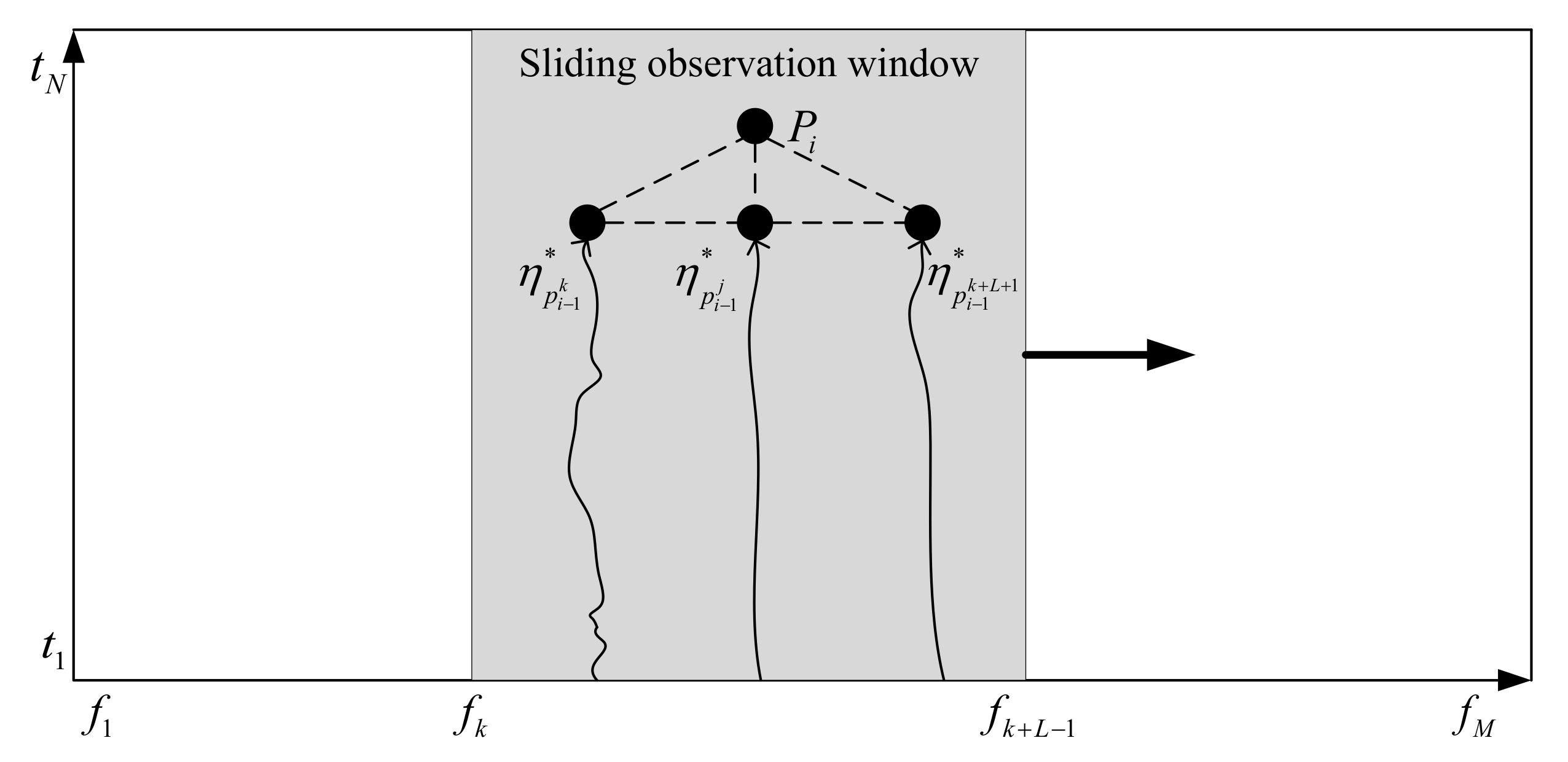
In this section, a sliding window line spectrum extraction algorithm based on multi-step decision is used to search for the optimal path. As shown in Figure 5, in this algorithm, a window which can slide along the frequency axis and cover the whole time axis is set in the LOFAR spectrum. We search the optimal path in this window. The reason for setting the window is that there may be multiple line spectrum co-existing in the LOFAR spectrum. By properly setting the size of the window, the search range of the path can be limited to a certain region of the LOFAR spectrum. Then the line spectrum in each window can be extracted, which can avoid that only the strongest spectral line is extracted in the whole LOFAR spectrum.
To cover a line spectrum in a search window, the size of the window is related to the line spectrum broadening and the frequency resolution in the LOFAR spectrum. The specific calculation steps are as follows:
- (1)
- The length of the frequency axis in the LOFAR spectrums M. The start point is , and the end point is . The length of the time axis is N. The start point is , and the end points . The search window size is defined as L.
- (2)
- Each point in the figure is defined as , representing the time-frequency pixel on the jth column on the frequency axis and the ith row on the time axis, where , . represents the optimal path from to in the observation window, defines as a set of ternary vectors for points , and the triplet of each point at is initialized to .
- (3)
- From to , find the optimal path with length from 2 to N in the search window line by line. In the figure, is set to any point in , the start position of the observation window is , and the corresponding end position is . At , the neighboring L points of form a set as follows, , the optimal path to the length i of the point is obtained from the optimal path of , i.e., , where satisfies:where represents the set of points .
- (4)
- At , the optimal path of the k points in the search window is , where , then the optimal path of length N in the search window is:
- (5)
- Set a counter for each time-frequency point in the LOFAR spectrum, and the counter value is initialized to 0. If the value of the objective function corresponding to the optimal path in the search window is greater than the threshold , we would consider that there is a line spectrum on the optimal path, and the counter values corresponding to the N points on the optimal path are increased by 1 respectively. The specific steps of threshold calculation are as follows:First, the input of the algorithm is changed from the LOFAR spectrum of ship radiation noise to the LOFAR spectrum of marine environmental noise. The corresponding cost function of the optimal path in the observation window is obtained, where then the threshold is:
- (6)
- Slide the search window with a step size of 1. Repeat the above steps until the observation window slides to the end. The output count value graph is the traced line spectrum.
4. Underwater Target-Recognition Framework Based on CNN
CNN has proven its powerful capability in many fields, such as pattern recognition, computer vision, nature language processing, and wireless physical layer [1,7,8,10]. It is composed of input layer, convolutional layer, activation function, pooling layer, and fully connected layer. The input layer can handle multi-dimensional data; similar to other neural networks, because of the use of gradient descent learning, the input features of CNN need to be standardized. The convolutional layer is used for feature extraction. The activation layer strengthens the expressive ability of the neural network. The pooling layer compresses the input features and extracts the main features [33,34,35]. The fully connected layer connects all the features and sends the output value to the classifier.
From the LOFAR spectrum of the measured underwater acoustic signal which is extracted through multi-step judgment, we design a convolutional neural network structure according to its characteristics. The specific network parameters can be seen in Table 1. For this CNN network structure, it refers some ideas of the inception module which uses different sizes of convolution kernels and weighs the characteristics of the global and local information distribution. This network structure selects different convolution kernels and pooling kernels for preliminary feature extraction. The output of each sub-layer is cascaded and passes through several convolutional layers and pooling layers. Finally, the flatten layer extends the feature map into vectors and the network completes the classification by the dense layer. Convolution and pooling performed in parallel in the network obtain features of different information scales. The network has strong feature extraction capabilities for the positional relationship of line spectrum on different frequency points in the LOFAR spectrum.
The network parameters of CNN have been marked in Table 1. means the size of the convolution kernel is , r means the number of channels. means the step size is . Conv and MaxPool are convolution layer and max pooling layer, respectively. CNN training and optimization hyperparameters are shown in Table 2.
Adam was originally proposed by Diederik Kingma of OpenAI and Jimmy Ba of the University of Toronto [36]. It is a first-order optimization algorithm that can replace the traditional stochastic gradient descent process. It can iteratively update neural network weights based on training data.
5. Numerical Results
5.1. Source of Experimental Data
The experimental data used in this article is divided into two parts: The first part of the underwater acoustic database is named ShipsEar [5], which was recorded by David et al. in the port of Vigo and it is vicinity on the Atlantic coast of northwestern Spain. The second part is based on the four types of signals simulated by the ship radiated noise. By mixing with the audio No. 81–92 in the database which are treated as the pure marine environment background noise, the simulated actual ship radiated noise under different signal-to-noise ratios is obtained.
Vigo Port is one of the largest ports in the world with a considerable cargo and passengers. Taking advantage of the high traffic intensity of the port and the diversity of ships, it can record the radiated noise of many different types of ships on the dock, including fishing boats, ocean liners, Roll-on/Roll-off ships, tugboats, yachts, small sailboats, etc. The ShipsEar database contains 11 ship types (marine environmental noise) and a total of 90 audio recordings in “wav” format, with audio lengths varying from 10 s to 11 min.
By extracting and summarizing audios in the database, it is divided into four categories according to the size of the ship types collected which is shown in Table 3. In addition, the date and weather conditions of the collected audios, the coordinates and driving status of the ship’s specific position, the number, depth and power gain of hydrophones, atmospheric and marine environmental data are also listed in detail. The information can be used as a reference in the study.
Because of military security considerations in the field of underwater target recognition, military databases are mostly kept secret. However, due to the inconvenience of collection and the high cost of civil databases, there are few public civilian databases for researchers to use. After the emergence of the ShipsEar database, it has been used in the application research of ship radiated noise separation, denoising, classification, etc. It is also common to use this database to complete research in the field of deep learning [18,19,20,21,37,38,39].
5.2. Experimental Software and Hardware Platform
The hardware platform and software support required to complete the deep-learning experiment are shown in Table 4.
During the whole experiment, we mainly use two pieces of software, Pycharm 2019.1 and MATLAB R2016B. Referring to Figure 1, we used MATLAB to complete the entire process of feature extraction. The algorithm in Section 3 is based on MATLAB for the calculation of LOFAR spectrum samples. For the algorithm in Section 4, we used Pycharm and Python to complete the task of CNN-based underwater target recognition. In addition, the depth library and software toolbox used are Keras (offline training and online testing), Librosa (all phasis) and TWQT (sampling and feature preprocessing).
5.3. Multi-Step Decision LOFAR Line Spectrum Enhancement Algorithm Validity Test
In this section, the audio data of ShipsEar (a database of measured ship radiated noise) is used to verify the effectiveness of the algorithm.
In the process of testing the effectiveness of the multi-step decision LOFAR line spectrum enhancement algorithm, morphological component analysis is required. In Section 2.1.1, we detailed the use of the RSSD algorithm to construct the optimal sparse representation of the high and low-resonance components in the ship radiated noise. In the RSSD algorithm, it is necessary to select an appropriate filter scaling factor according to the waveform characteristics of the signal, to calculate the parameters corresponding to the two types of resonance components, and construct the corresponding wavelet basis functions. In this regard, we have completed the calculation of the parameters with the help of MATLAB. For the signal decomposition algorithm based on resonance, the parameters setting for extracting high-resonance components are , , , and the parameters setting for extracting low-resonance components are , , . The energy distribution of the low-resonance component signal and the high-resonance component signal is finally calculated as follows:
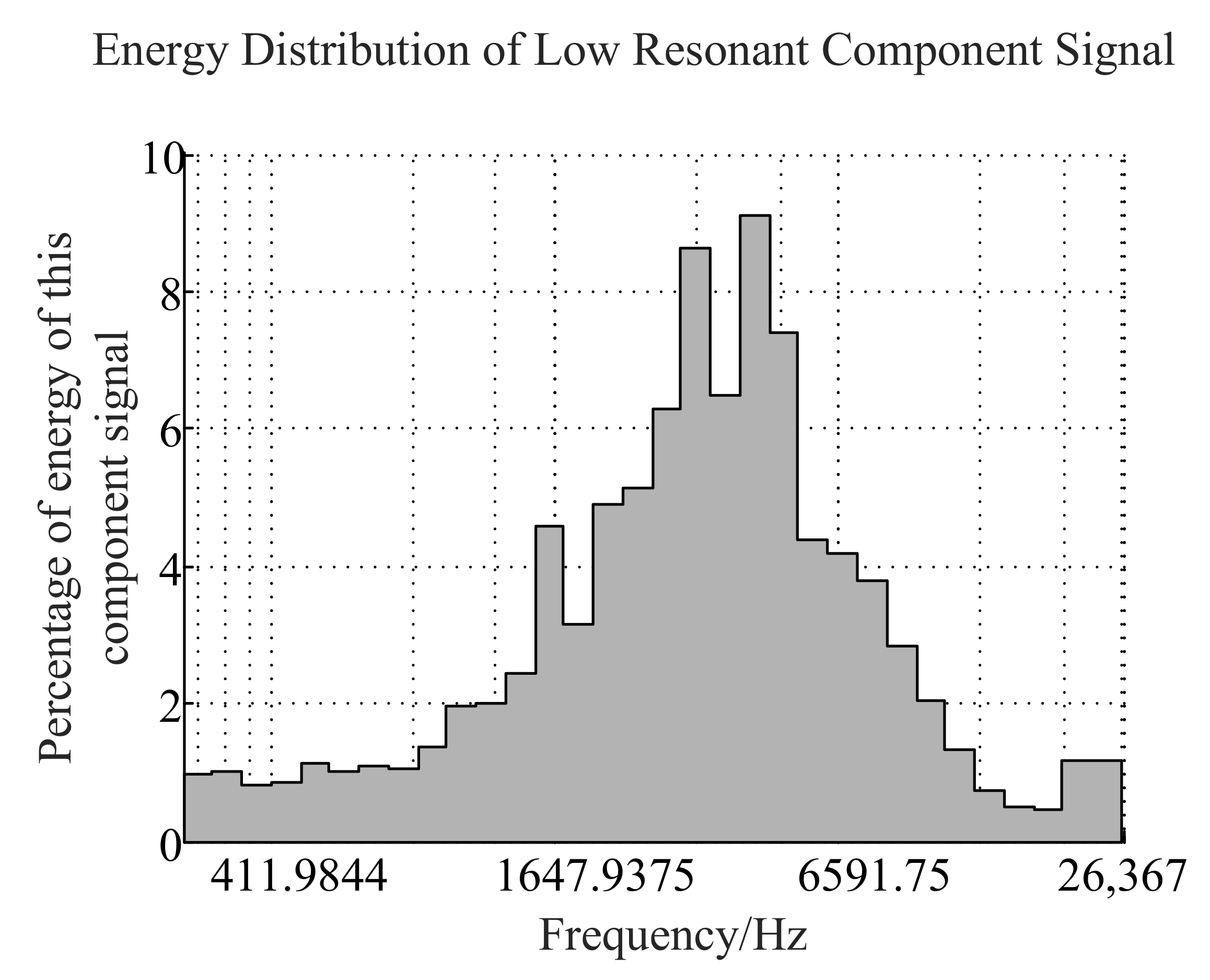
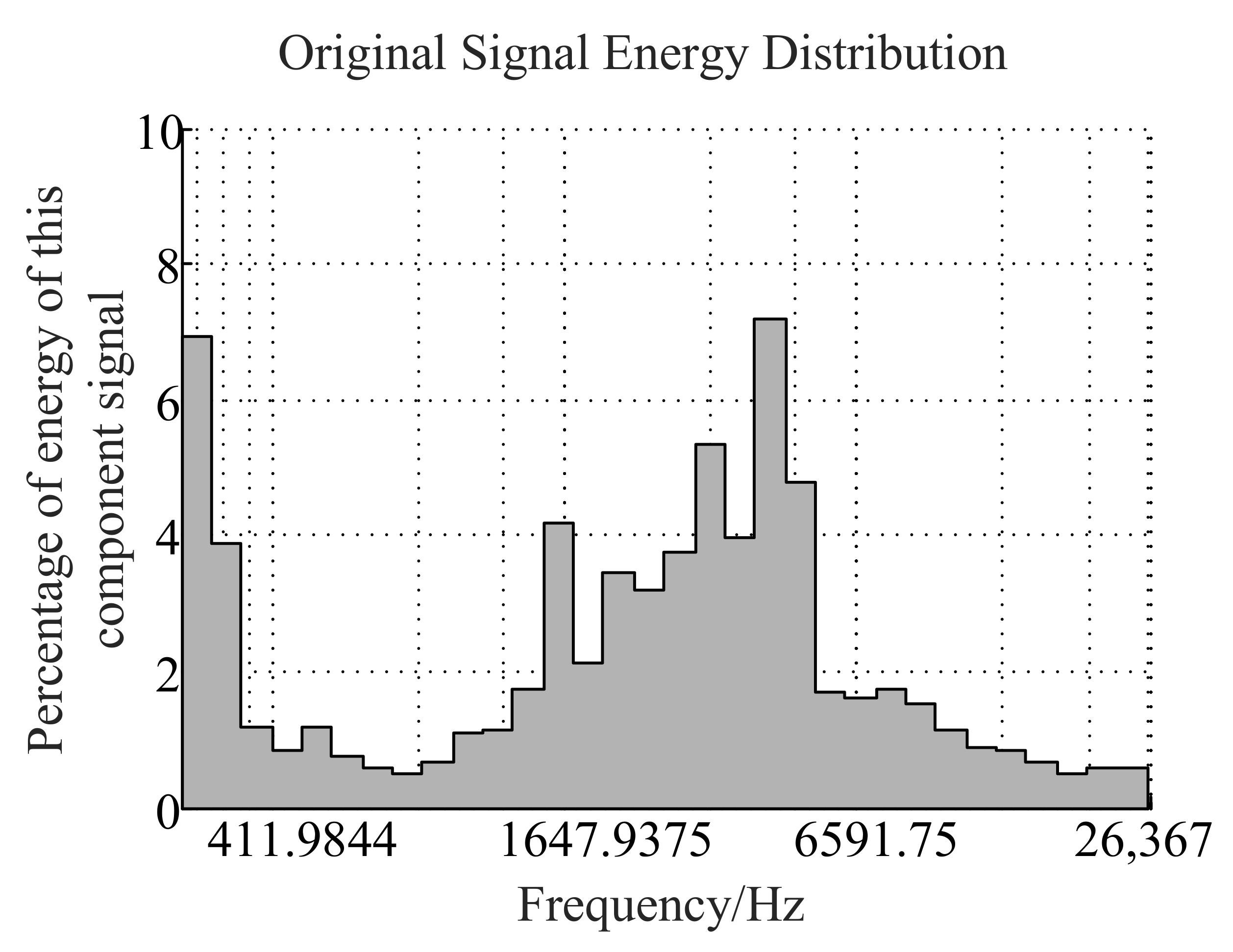
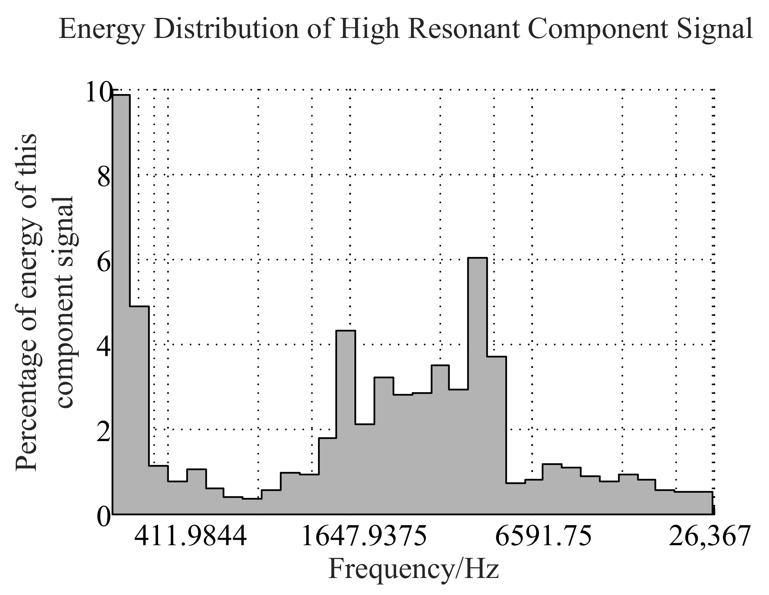
From the energy percentage of each frequency band in Figure 6, the energy distribution of the low-resonance component is mostly concentrated in the higher frequency band (greater than 1000 Hz), while the energy distribution in the low-frequency band is very small. Compared to Figure 7, we find that higher energy distribution of the original signal comes from the low-resonance component. In Figure 8, most of the energy of the high-resonance component is concentrated in the low-frequency narrow band, and the narrow band energy distribution characteristic is usually regarded as a line spectrum. In previous studies, the low-frequency line spectrum is the main manifestation of mechanical noise and propeller cavitation noise in the LOFAR spectrum. It is also an important basis for the identification of ship radiated noise. Therefore, the separated high-resonance component retains the main features of underwater target recognition well.
In addition, Spectral Correlation Coefficient (SCC) [40] can also be used to measure the effectiveness of the RSSD algorithm. The physical significance of the spectral correlation coefficient is measuring the similarity of the power spectrum of the two signals, which is defined as follows:
where and represent the power spectrum of the two types of signals A and B, respectively. and represent the range of the power spectrum. This means that the radiated noise of the two types of ships with a higher degree of difference has a smaller spectral correlation coefficient. It can be seen from Table 5 that the spectral correlation coefficients in the high-resonance components of signals A and B are smaller than their original spectral correlation coefficients. It means we can enhance the degree of difference between the two signals by extracting the high-resonance components of the signal.
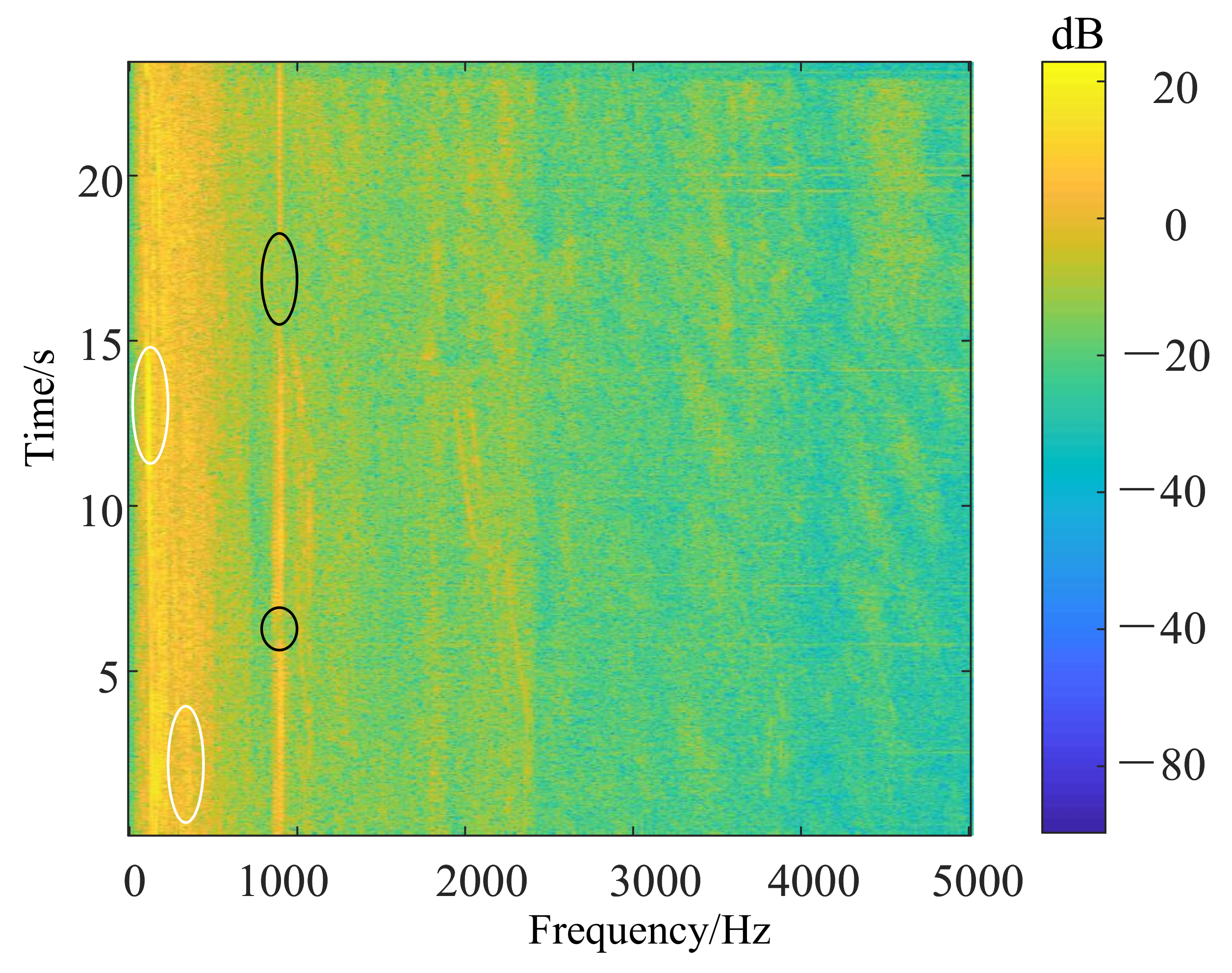
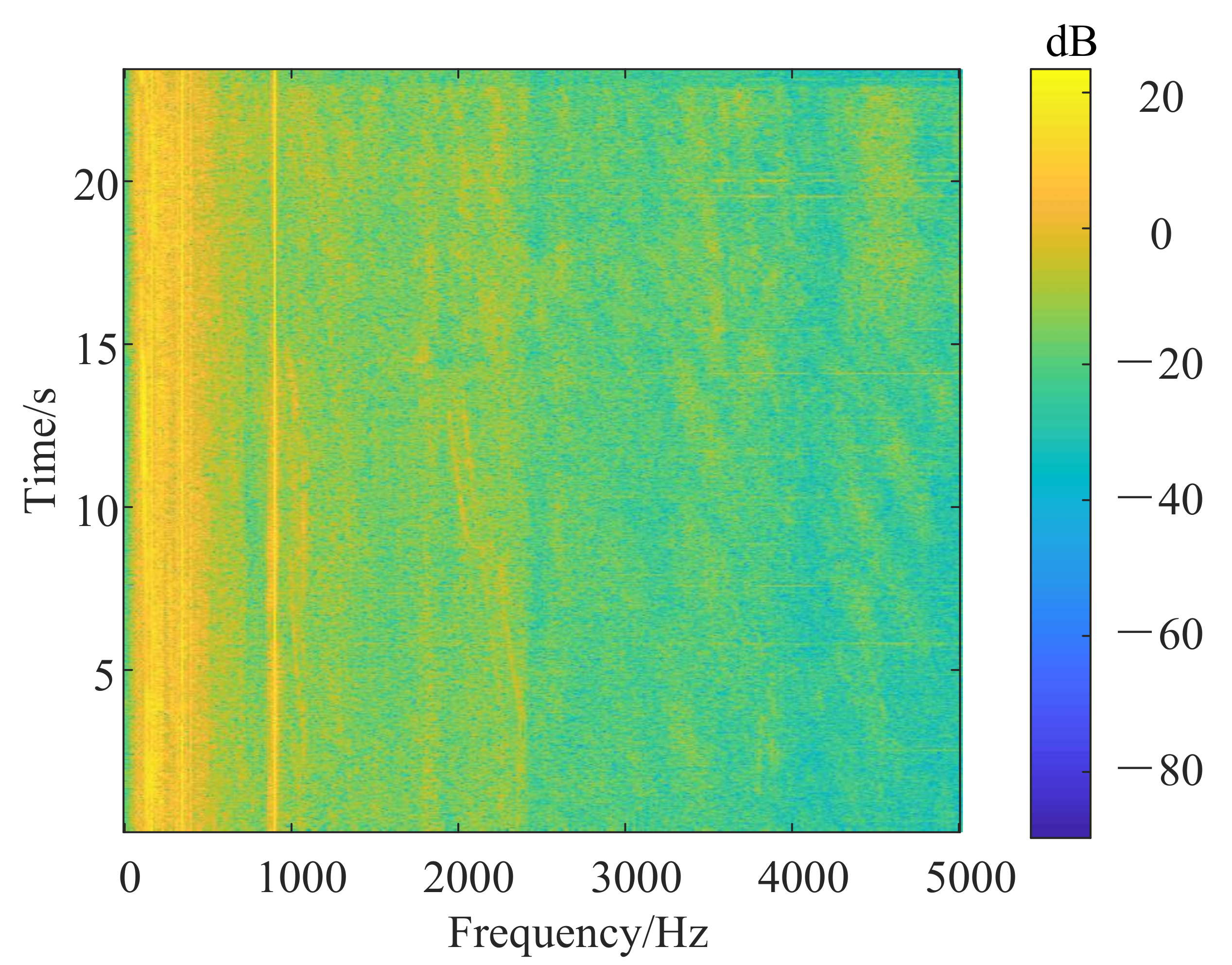
For the line spectrum enhancement algorithm based on multi-step decision, the experimental results are shown in Figure 9 and Figure 10, which are the LOFAR spectrum of the original signal and the LOFAR spectrum after line spectrum enhancement. In Figure 9, there is an obvious line spectrum in the part marked by white circles, but the line spectrum is broken in the part marked by black circles. In Figure 10, the line spectrum indicated by the white circles are extended to completeness, and the vacant part of the line spectrum indicated by the black circles is also completed. Therefore, even if the line spectrum in the LOFAR spectrum has “breakpoints”, “broken lines” or only a short line due to noise interference, the line spectrum enhancement algorithm can still extend and complete the line spectrum.
5.4. Experimental Verification of Underwater Target Recognition Based on Convolutional Neural Network (CNN)
5.4.1. CNN Network Offline Training Process
According to the frame structure of underwater target recognition in Figure 1, the specific settings and steps can be divided into:
- (1)
- Read the high-resonance component signals in sequence, then windowing and framing the signal. We choose Hanning window (Hanning), and the window size is 2048 (i.e., FFT points are 2048). The overlap between frames is 75%.
- (2)
- The signal of each frame is normalized and decentralized. The power of the signal is uniform in time and the average value of the sample is 0. It means the data are limited to a certain range, which can eliminate singular sample data. At the same time, it can also avoid the saturation of neurons and accelerate the convergence rate of the network.
- (3)
- First, perform Fourier transform on each frame signal. Second, take the logarithmic amplitude spectrum of the transformed spectrum and arrange it in the time domain. Last, take 64 points on the time axis as a sample, which means obtaining a size of LOFAR spectrum sample. The sampling frequency of audio is 52,734 Hz, and the duration of each sample is about s. The numbers of training and testing sets of various samples are shown in Table 6. The ID in the table is the label of the audio in the ShipsEar database. The corresponding type of ship for each segment can be obtained according to the ID. The type of ship corresponding to audio is used as a label for supervised learning of deep neural networks.
- (4)
- The sample obtained in step (3) is treated with LOFAR spectrum enhancement. The specific sample processing process and calculation process are in Section 3.3. Then the LOFAR spectrum with enhanced line spectrum characteristics is obtained. The LOFAR spectrum is a two-dimensional matrix, which can be regarded as a single-channel image. After that as shown in Figure 1, the data enhanced by the multi-step decision LOFAR spectrum is input into the CNN network for subsequent identification.
5.4.2. Identification of Measured Ship Radiated Noise
The testing data set adopts the same feature preprocessing as the training set and inputs the trained model to complete the test.
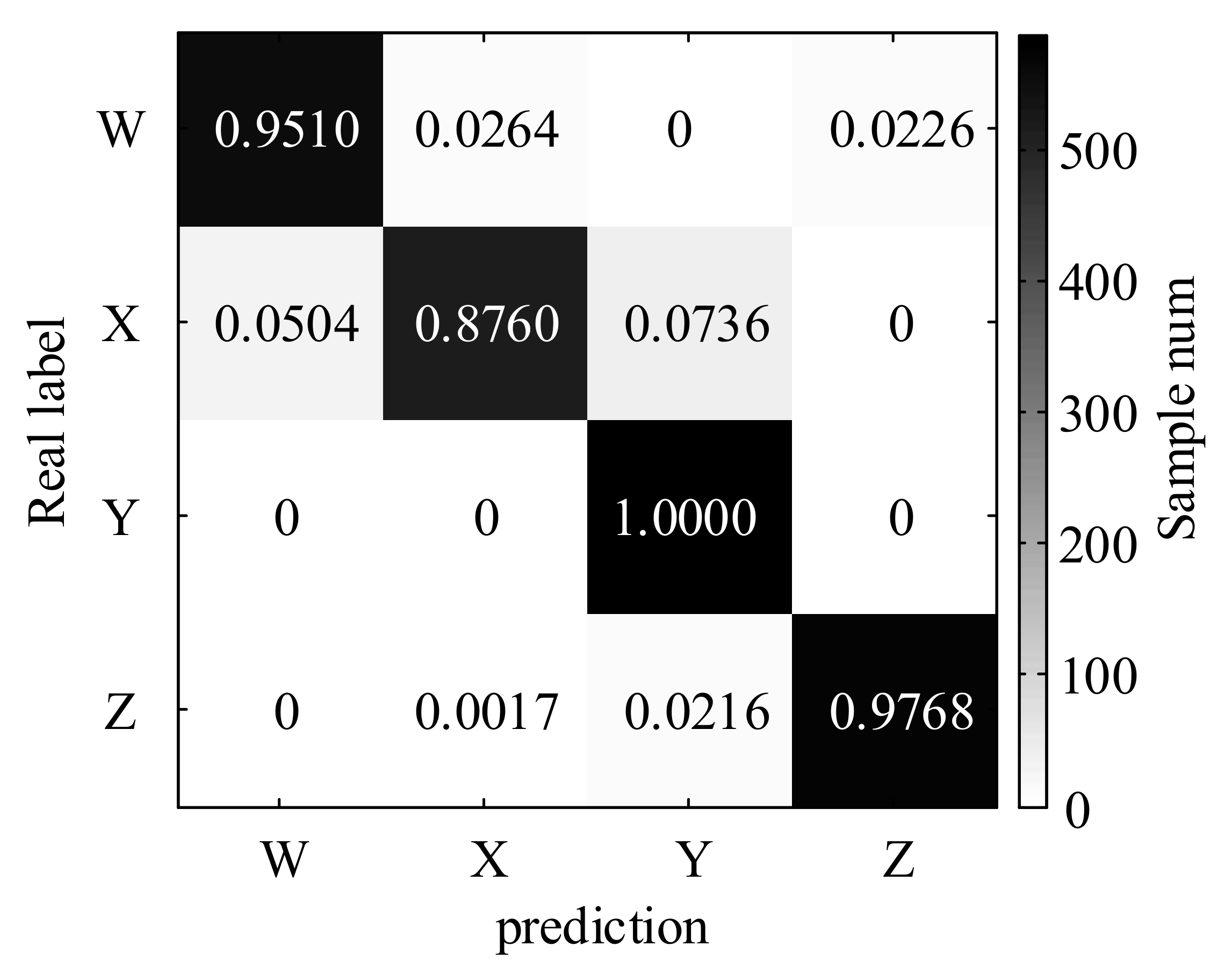
Figure 11 shows the standardized confusion matrix. The recognition accuracy of the radiated noise of the four types of ships is different. Among them, the recognition effect of the Y-signal is the best and the recognition accuracy rate reaches 100.00%. The recognition accuracy rates of the W-type and Z-type are slightly worse, and they are 95.10% and 97.68%. Additionally, the recognition effect of the X-type is the worst, which is only 87.60%. In summary, the total recognition accuracy rate is 95.22%. The recognition accuracy of four kinds of measured ship radiated noise is shown in Table 7.
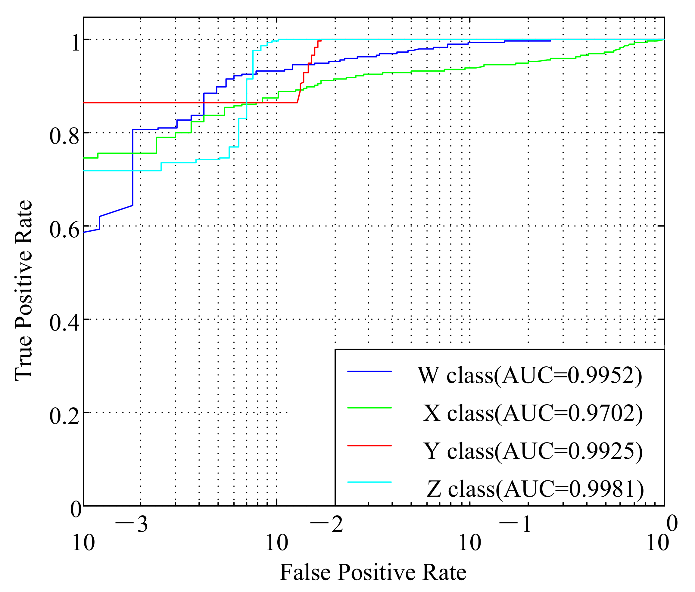
Figure 12 shows the ROC curve and the corresponding AUC value of the four types of signals. The horizontal axis uses a logarithmic scale to enlarge the ROC curve in the upper left corner. The ROC curves of the signals of W, Y, and Z are relatively close to the point, and their classification effects are relatively good. However, the ROC curve of the signals of type X is closest to the 45-degree line, so the classification effect is worst. Judging from the AUC value, the AUC of the Z-type signal is the highest, which reaches . The AUC values of the W-type and Y-type signals have respectively reached and . The AUC value of the X-type signal is only . Therefore, the classification effect of the X-type signal is also inferior to the other three types of signals.
6. Conclusions
In this paper, we have studied underwater target recognition using the LOFAR spectrum. First, a deep-learning underwater target-recognition framework based on multi-step decision LOFAR line spectrum enhancement is developed, in which we use CNN for offline training and online testing. Under the developed underwater target-recognition framework, we then use the LOFAR spectrum as the input of CNN. In particular, on calculating the LOFAR spectrum of the high-resonance component, we use the algorithm based on resonance and design the LOFAR spectrum line enhancement algorithm which is based on multi-step decision. To the best of our knowledge, the difference between the radiated noise of different types of ships is enhanced, and the broken line spectrum can be detected and enhanced. Finally, we conduct extensive experiments in terms of the detection performance, scalability, and complexity. The results have shown that the LOFAR-CNN method can achieve the highest recognition rate of 95.22% with the measured ship radiation noise which can further improve the recognition accuracy compared with other traditional method.
7. Future Works
This paper uses deep-learning methods to provide a framework to realize underwater target recognition. This algorithm shows excellent underwater target-recognition ability, and has great application value in many aspects such as seabed exploration, oil platform monitoring and economic fish detection. It can not only predict dangerous objects in advance, improve the safety of ship navigation, but also create greater economic benefits. However, there are still some shortcomings that need to be resolved.
- (1)
- Most studies on underwater target recognition do not disclose data sources for reasons such as confidentiality. There is also a lack of unified and standardized data sets in the industry. The actual measured ship radiated noise data set used in this article is already one of the few publicly available underwater acoustic data sets. However, the data set itself is seriously disturbed by marine environmental noise. The number of samples of various types of ships is unevenly distributed, and the total number of samples is also insufficient. Therefore, how to combine underwater target recognition with deep learning under limited conditions is a big problem.
- (2)
- Because the data set is seriously disturbed, this paper adopts a series of feature-enhancing preprocessing methods to improve the recognition rate, and has achieved excellent results. In fact, further reducing the impact of ocean noise and evaluating the impact of various neural networks on the recognition effect can be considered in the future work.
Author Contributions
Conceptualization, J.C.; methodology, J.C., B.H., X.M. and J.Z.; software, B.H. and X.M.; validation, B.H. and X.M.; formal analysis, J.C. and B.H.; investigation, J.C. and B.H.; resources, J.C. and B.H.; data curation, J.C., B.H., X.M. and J.Z.; writing—original draft preparation, J.C. and B.H.; writing—review and editing, J.C. and B.H.; visualization, J.C. and B.H.; supervision, J.C.; project administration, J.C.; funding acquisition, J.C. All authors have read and agreed to the published version of the manuscript.
Funding
This research was funded by the China National Key R&D Program under grant 2020YFB1807700.
Data Availability Statement
Not Applicable, the study does not report any data.
Conflicts of Interest
The authors declare no conflict of interest.
References
- Xie, J.; Fang, J.; Liu, C.; Li, X. Deep learning-based spectrum sensing in cognitive radio: A CNN-LSTM approach. IEEE Commun. Lett. 2020, 24, 2196–2200. [Google Scholar] [CrossRef]
- Liu, C.; Yuan, W.; Li, S.; Liu, X.; Ng, D.W.K.; Li, Y. Learning-based Predictive Beamforming for Integrated Sensing and Communication in Vehicular Networks. arXiv 2021, arXiv:2108.11540. [Google Scholar]
- Xie, J.; Fang, J.; Liu, C.; Yang, L. Unsupervised deep spectrum sensing: A variational auto-encoder based approach. IEEE Trans. Veh. Technol. 2020, 69, 5307–5319. [Google Scholar] [CrossRef]
- Hubel, D.H.; Wiesel, T.N. Receptive fields, binocular interaction and functional architecture in the cat’s visual cortex. J. Phy. 1962, 160, 106–154. [Google Scholar] [CrossRef]
- Santos-Domínguez, D.; Torres-Guijarro, S.; Cardenal-López, A.; Pena-Gimenez, A. ShipsEar: An underwater vessel noise database. Appl. Acoust. 2016, 113, 64–69. [Google Scholar] [CrossRef]
- Ciaburro, G.; Iannace, G. Improving Smart Cities Safety Using Sound Events Detection Based on Deep Neural Network Algorithms. Informatics 2020, 7, 23. [Google Scholar] [CrossRef]
- Liu, C.; Wei, Z.; Ng, D.W.K.; Yuan, J.; Liang, Y.C. Deep transfer learning for signal detection in ambient backscatter communications. IEEE Trans. Wirel. Commun. 2020, 20, 1624–1638. [Google Scholar] [CrossRef]
- Ciaburro, G. Sound Event Detection in Underground Parking Garage Using Convolutional Neural Network. Big Data Cogn. Comput. 2020, 4, 20. [Google Scholar] [CrossRef]
- Goodfellow, I.; Bengio, Y.; Courville, A.; Bengio, Y. Deep Learning; MIT Press: Cambridge, UK, 2016. [Google Scholar]
- Liu, C.; Wang, J.; Liu, X.; Liang, Y.C. Deep CM-CNN for spectrum sensing in cognitive radio. IEEE J. Sel. Areas Commun. 2019, 37, 2306–2321. [Google Scholar] [CrossRef]
- LeCun, Y.; Boser, B.E.; Denker, J.S.; Henderson, D.; Howard, R.E.; Hubbard, W.E.; Jackel, L.D. Handwritten digit recognition with a back-propagation network. In Proceedings of the Handwritten Digit Recognition with a Back-Propagation Network. Advances in Neural Information Processing Systems, Denver, CO, USA, 27–30 November 1989; pp. 396–404. Available online: https://proceedings.neurips.cc/paper/1989/file/53c3bce66e43be4f209556518c2fcb54-Paper.pdf (accessed on 4 October 2021).
- Szegedy, C.; Liu, W.; Jia, Y.; Sermanet, P.; Reed, S.; Anguelov, D.; Erhan, D.; Vanhoucke, V.; Rabinovich, A. Going deeper with convolutions. In Proceedings of the IEEE Conference on Computer Vision and Pattern Recognition (CVPR), Boston, MA, USA, 7–12 June 2015; pp. 1–9. [Google Scholar]
- Szegedy, C.; Vanhoucke, V.; Ioffe, S.; Shlens, J.; Wojna, Z. Rethinking the inception architecture for computer vision. In Proceedings of the IEEE Conference on Computer Vision and Pattern Recognition (CVPR), Las Vegas, NV, USA, 27–30 June 2016; pp. 2818–2826. [Google Scholar]
- Szegedy, C.; Ioffe, S.; Vanhoucke, V.; Alemi, A.A. Inception-v4, inception-resnet and the impact of residual connections on learning. In Proceedings of the Thirty-first AAAI conference on artificial intelligence (AAAI), San Francisco, CA, USA, 4–9 February 2017; pp. 4278–4284. [Google Scholar]
- He, K.; Zhang, X.; Ren, S.; Sun, J. Deep residual learning for image recognition. In Proceedings of the IEEE conference on computer vision and pattern recognition (CVPR), Las Vegas, NV, USA, 17–19 June 2016; pp. 770–778. [Google Scholar]
- Jin, G.; Liu, F.; Wu, H.; Song, Q. Deep learning-based framework for expansion, recognition and classification of underwater acoustic signal. J. Exp. Theor. Artif. Intell. 2019, 32, 205–218. [Google Scholar] [CrossRef]
- Liu, F.; Song, Q.; Jin, G. Expansion of restricted sample for underwater acoustic signal based on generative adversarial networks. May 2019. In Proceedings of the Tenth International Conference on Graphics and Image Processing (ICGIP), Chengdu, China, 12–14 December 2018; Volume 11069, pp. 1106948–1106957. [Google Scholar]
- Yang, H.; Shen, S.; Yao, X.; Sheng, M.; Wang, C. Competitive deep-belief networks for underwater acoustic target recognition. Sensors 2018, 18, 952–965. [Google Scholar] [CrossRef] [Green Version]
- Shen, S.; Yang, H.; Sheng, M. Compression of a deep competitive network based on mutual information for underwater acoustic targets recognition. Entropy 2018, 20, 243–256. [Google Scholar] [CrossRef] [PubMed] [Green Version]
- Yan, J.; Sun, H.; Chen, H.; Junejo, N.U.R.; Cheng, E. Resonance-based time-frequency manifold for feature extraction of ship-radiated noise. Sensors 2018, 18, 936–957. [Google Scholar] [CrossRef] [Green Version]
- Ke, X.; Yuan, F.; Cheng, E. Underwater Acoustic Target Recognition Based on Supervised Feature-Separation Algorithm. Sensors 2018, 18, 4318–4342. [Google Scholar] [CrossRef] [PubMed] [Green Version]
- Zhu, P.; Isaacs, J.; Fu, B.; Ferrari, S. Deep learning feature extraction for target recognition and classification in underwater sonar images. In Proceedings of the 2017 IEEE 56th Annual Conference on Decision and Control CDC), Melbourne, Australia, 12–15 December 2017; pp. 2724–2731. [Google Scholar]
- McQuay, C.; Sattar, F.; Driessen, P.F. Deep learning for hydrophone big data. In Proceedings of the 2017 IEEE Pacific Rim Conference on Communications, Computers and Signal Processing (PACRIM), Victoria, QC, Canada, 21–23 August 2017; pp. 1–6. [Google Scholar]
- Hu, G.; Wang, K.; Peng, Y.; Qiu, M.; Shi, J.; Liu, L. Deep learning methods for underwater target feature extraction and recognition. Comput. Intell. Neurosci. 2018, 2018, 1–10. [Google Scholar] [CrossRef]
- Kubáčková, L.; Burda, M. Mathematical model of the spectral decomposition of periodic and non-periodic geophysical stationary random signals. Stud. Geophys. Geod. 1977, 21, 1–10. [Google Scholar] [CrossRef]
- Huang, W.; Sun, H.; Liu, Y.; Wang, W. Feature extraction for rolling element bearing faults using resonance sparse signal decomposition. Exp. Tech. 2017, 41, 251–265. [Google Scholar] [CrossRef]
- Selesnick, I.W. Wavelet transform with tunable Q-factor. IEEE Trans. Signal Process. 2011, 59, 3560–3575. [Google Scholar] [CrossRef]
- Starck, J.L.; Elad, M.; Donoho, D.L. Image decomposition via the combination of sparse representations and a variational approach. IEEE Trans. Image Process. 2005, 14, 1570–1582. [Google Scholar] [CrossRef] [PubMed] [Green Version]
- Al-Raheem, K.F.; Roy, A.; Ramachandran, K.; Harrison, D.K.; Grainger, S. Rolling element bearing faults diagnosis based on autocorrelation of optimized: Wavelet de-noising technique. Int. J. Adv. Manuf. Technol. 2009, 40, 393–402. [Google Scholar] [CrossRef]
- Shensa, M.J. The discrete wavelet transform: Wedding the a trous and Mallat algorithms. IEEE Trans. Signal Process. 1992, 40, 2464–2482. [Google Scholar] [CrossRef] [Green Version]
- Wang, H.; Chen, J.; Dong, G. Feature extraction of rolling bearing’s early weak fault based on EEMD and tunable Q-factor wavelet transform. Mech. Syst. Signal Proc. 2014, 48, 103–119. [Google Scholar] [CrossRef]
- Di Martino, J.C.; Haton, J.P.; Laporte, A. Lofargram line tracking by multistage decision process. In Proceedings of the 1993 IEEE International Conference on Acoustics, Speech and Signal Processing (ICASSP), Minneapolis, MN, USA, 27–30 April 1993; Volume 1, pp. 317–320. [Google Scholar]
- Liu, C.; Liu, X.; Ng, D.W.K.; Yuan, J. Deep Residual Learning for Channel Estimation in Intelligent Reflecting Surface-Assisted Multi-User Communications. IEEE Trans. Wirel. Commun. 2021, 1. [Google Scholar] [CrossRef]
- Liu, X.; Liu, C.; Li, Y.; Vucetic, B.; Ng, D.W.K. Deep residual learning-assisted channel estimation in ambient backscatter communications. IEEE Wirel. Commun. Lett. 2020, 10, 339–343. [Google Scholar] [CrossRef]
- Liu, C.; Yuan, W.; Wei, Z.; Liu, X.; Ng, D.W.K. Location-aware predictive beamforming for UAV communications: A deep learning approach. IEEE Wirel. Commun. Lett. 2020, 10, 668–672. [Google Scholar] [CrossRef]
- Kingma, D.P.; Ba, J. Adam: A Method for Stochastic Optimization. arXiv 2014, arXiv:1412.6980. [Google Scholar]
- Chen, Z.; Li, Y.; Cao, R.; Ali, W.; Yu, J.; Liang, H. A New Feature Extraction Method for Ship-Radiated Noise Based on Improved CEEMDAN, Normalized Mutual Information and Multiscale Improved Permutation Entropy. Entropy 2019, 21, 624–640. [Google Scholar] [CrossRef] [Green Version]
- Yuan, F.; Ke, X.; Cheng, E. Joint Representation and Recognition for Ship-Radiated Noise Based on Multimodal Deep Learning. J. Mar. Sci. Technol. Eng. 2019, 7, 380–397. [Google Scholar] [CrossRef] [Green Version]
- Ke, X.; Yuan, F.; Cheng, E. Integrated optimization of underwater acoustic ship-radiated noise recognition based on two-dimensional feature fusion. Appl. Acoust. 2020, 159, 107057–107070. [Google Scholar] [CrossRef]
- Hou, W. Spectrum autocorrelation. Acta Acust 1988, 2, 46–49. [Google Scholar]
Figure 1.
Deep-learning underwater target-recognition framework based on multi-step decision LOFAR line spectrum enhancement.
Figure 1.
Deep-learning underwater target-recognition framework based on multi-step decision LOFAR line spectrum enhancement.

Figure 2.
Signal decomposition algorithm based on resonance.

Figure 3.
Analysis filter bank.

Figure 4.
Integrated filter bank.

Figure 5.
Frequency-domain sliding window multi-step decision dynamic tracking line spectrum.

Figure 6.
Percentage of total energy of each frequency band of low-resonance component signal.

Figure 7.
The percentage of total energy of each frequency band of the original signal.

Figure 8.
Percentage of total energy of each frequency band of high-resonance component signal.

Figure 9.
LOFAR spectrum of the original signal.

Figure 10.
LOFAR spectrum after line spectrum enhancement.

Figure 11.
Confusion matrix of four types of measured ship radiated noise under CNN.

Figure 12.
The ROC curve and AUC value of four types of measured ship radiated noise under CNN.


Table 1.
The CNN network model parameters of measured dataset.
| Input Layer (1024) × 64 × 1 | ||||
|---|---|---|---|---|
| Conv+ ReLU (7 × 7) × 16 stride = 2 × 1 | Conv+ ReLU (7 × 5) × 16 stride = 2 × 1 | Conv+ ReLU (5 × 5) × 16 stride = 2 × 1 | Conv+ ReLU (3 × 3) × 16 stride = 2 × 1 | MaxPool (3 × 3) Conv+ReLU (1 × 1) × 16 stride = 1 × 1 |
| Fileter concatenation | ||||
| ReLU+MaxPool (3 × 3) | ||||
| Conv+ReLU(5 × 5) × 16 stride = 2 × 1 | ||||
| MaxPool (3 × 3) | ||||
| Conv+ReLU(5 × 5) × 16 stride = 2 × 1 | ||||
| MaxPool (3 × 3) | ||||
| Conv+ReLU (3 × 3) × 32 stride = 2 × 2 | ||||
| MaxPool (3 × 3) | ||||
| Flattern | ||||
| Dense (4) | ||||
Table 2.
CNN training, optimization hyperparameters.
| Item | Value |
|---|---|
| Optimizer | adam |
| Learning rate | 0.01 |
| Number of samples | 200 |
| Training round | 30 |
| Loss function | Cross entropy loss function |
Table 3.
Four types of ship targets.
| Item | Value |
|---|---|
| W | Fishing boat, trawler, mussel harvester, tugboat, dredge |
| X | Motorboat, pilot boat, sailboat |
| Y | Passenger ferry |
| Z | Ocean liner, ro-ro ship |
Table 4.
Experimental hardware platform and software support.
| Lab Environment | Configuration |
|---|---|
| Operating system | Ubuntu 16.04 |
| Graphics card | GTX 1080ti |
| Programming language and software | Pycharm 2019.1 + Python 3.6 |
| Matlab R2016b | |
| Deep-learning library and software toolbox | Keras 2.3 (tensorflow backed) |
| Librosa Audio processing library (python) | |
| TQWT Toolbox (Matlab language) |
Table 5.
Spectral correlation coefficients between the two types of original signals and their high-resonance components.
Table 5.
Spectral correlation coefficients between the two types of original signals and their high-resonance components.
| Signal | , | , |
|---|---|---|
| 0.7161 | 0.7074 |
Table 6.
Various sample training sets and testing sets.
| ID | Training Set | Testing Set | |
|---|---|---|---|
| Number of Samples | Number of Samples | ||
| W | 46, 48, 66, 73, 74, 75, 80, 93, 94, 95, 96 | 836 | 531 |
| X | 21, 26, 29, 30, 50, 52, 57, 70, 72, 77, 79 | 837 | 516 |
| Y | 6, 7, 8, 10, 11, 13, 14 | 1016 | 526 |
| Z | 18, 19, 20 | 1149 | 603 |
| Total | 3838 | 2176 |
Table 7.
The recognition accuracy rate of the four types of measured ship radiated noise.
| Recognition Rate | Class W | Class X | Class Y | Class Z | Average |
|---|---|---|---|---|---|
| CNN | 95.10% | 87.60% | 100.0% | 97.78% | 95.22% |
Publisher’s Note: MDPI stays neutral with regard to jurisdictional claims in published maps and institutional affiliations. |
© 2021 by the authors. Licensee MDPI, Basel, Switzerland. This article is an open access article distributed under the terms and conditions of the Creative Commons Attribution (CC BY) license (https://creativecommons.org/licenses/by/4.0/).
Share and Cite
MDPI and ACS Style
Chen, J.; Han, B.; Ma, X.; Zhang, J. Underwater Target Recognition Based on Multi-Decision LOFAR Spectrum Enhancement: A Deep-Learning Approach. Future Internet 2021, 13, 265. https://0-doi-org.brum.beds.ac.uk/10.3390/fi13100265
AMA Style
Chen J, Han B, Ma X, Zhang J. Underwater Target Recognition Based on Multi-Decision LOFAR Spectrum Enhancement: A Deep-Learning Approach. Future Internet. 2021; 13(10):265. https://0-doi-org.brum.beds.ac.uk/10.3390/fi13100265
Chicago/Turabian StyleChen, Jie, Bing Han, Xufeng Ma, and Jian Zhang. 2021. "Underwater Target Recognition Based on Multi-Decision LOFAR Spectrum Enhancement: A Deep-Learning Approach" Future Internet 13, no. 10: 265. https://0-doi-org.brum.beds.ac.uk/10.3390/fi13100265
Note that from the first issue of 2016, this journal uses article numbers instead of page numbers. See further details here.