1. Introduction
Road transportation represents a major activity in the logistics of the agricultural sector. It plays an important role in stakeholder satisfaction [
1] and it is necessary for economic development. However, it also has an enormous impact on human health and the environment. Conventional vehicles use fuel engines, which are crucial sources of CO
2, N
2O, greenhouse gases (GHGs) [
2], and negative externalities, including air pollution, noise, accidents, traffic congestions, climate change risk, and resource consumption [
3]. According to Arias et al. (2018) [
4], non-renewable energy sources that release GHGs account for 14% of global pollution. Thus, in the last decade, green logistics with green energy sources have received increased attention intending to minimize harmful effects on the environment. Electric vehicles (EVs) have become more attractive solutions to environmental problems via green technology. Many logistics companies have started projects for the implementation of EVs in their operations, such as UPS and DHL [
5].
EVs have some benefits over traditional internal combustion engine vehicles (ICEVs). Firstly, EVs are the best alternative for greener transportation in the city and urban areas because they have zero GHGs emissions if their electricity comes from a renewable source. They also feature a significant reduction of air and noise pollution. However, EVs have limited driving ranges in comparison with ICEVs. The range of an EV depends on the electricity volume stored in the battery. Fast chargers are not a practical option for transportation trucks since the charging stations are still insufficient [
6]. The improvement of battery efficiency to extend the driving range is obstructed by concerns related to cost, the availability of materials, and safety [
7]. These reasons imply that the situation of driving range limitation for EVs will not likely change in the coming year. Thus, it is still a greater challenge to consider the restricted driving range for EVs because of insufficient supporting systems.
In recent research, some papers have focused on locating recharging stations or battery swap stations concurrently with routing decisions. Additionally, those papers considered the product delivery with a single depot location routing problem, a solution which impractically deals with real scenarios. Consequently, this paper intends to fulfill this gap and address realistic planning characteristics. This research not only determines locating multiple depots and assigning customers to them but also decides to route information for EVs with restricted driving ranges. This model is constructed for the planning aspect of a single echelon location routing problem, whereas previous studies have focused on the facilities for recharging and battery swap station.
Cassava is the main economic crop of Thailand and generates huge income for the country. Currently, Thailand is the third-largest cassava producer globally, after Nigeria and Congo, but Thailand is the leading global exporter [
8]. In 2017, Thailand produced 30.5 million tons of cassava, accounting for 9% of the world’s production, and the exporting value was 80,000 million baht [
9]. Thailand has cassava planting areas that spread throughout every region of the country, where the total planting area is 8.9 million rai (1 rai = 0.16 ha) [
10]. Because of the wide planting area, farmers must deal with a high transportation cost, especially when the distances between farms and buyers are far. Cassava farmers are facing constraints that reduce their income, owing to higher transportation costs, higher fuel prices, and additional price fluctuations. The current transportation system is still insufficient to support farmers. The government has focused on a policy surrounding this problem by supporting the establishment of collection centers. These centers will be standardized markets that set the standard price for buying a product, thereby farmers who live far away can save on transportation costs and receive fairness from selling products. Moreover, the suitable location of the center and economic routing will enhance the efficiency of the transportation system. Therefore, this research study focuses on finding the locations of collection centers and routing vehicles to pick up and deliver cassava to said centers.
In developing countries, the agricultural sector typically lacks technologies to improve productivity and maximize crop yield. The motivation of this research is to provide a feasibility study for the integration of increasing farmer’s profitability via the technological benefits of EVs. The main contributions of this research study are threefold. Firstly, this paper proposes a new electric vehicle location routing problem (EVLRP) model, which is unique in terms of its planning aspects when compared to the previous literature on location routing problems (LRPs) dealing with EVs. Secondly, the model is formulated from a real case problem in Thailand. Besides, the model includes a realistic constraint, i.e., that the cassava quantity at the farm might exceed the vehicle capacity, thus the farm has a chance to be served more than once by applying a partial shipment with full vehicle capacity, then providing routing for the remaining quantity. Thirdly, the proposed adaptive large neighborhood search (ALNS) algorithm provides four combinations of different acceptance criteria for benchmarking. Then, the best one is selected for application to the case study.
This paper is constructed as follows: A literature review is prepared in
Section 2.
Section 3 presents the problem description and mathematical model.
Section 4 introduces the ALNS methodology for solving this problem, while the computational results and their analysis are revealed in
Section 5. Finally, conclusions and suggestions for future work are given in
Section 6.
2. Literature Review
The literature review is composed of two main streams of research correlated with this work. The first stream concerns green location routing problems where no EV is used. Location routing problems (LRPs) integrate the facility location problems (FLPs) with vehicle routing problems (VRPs). Both FLPs and VRPs are NP-hard problems [
11]. Therefore, LRPs also consider NP-hard combinatorial optimization problems [
12]. Many authors have studied LRP in variants of green transportation. Toro et al. (2017) [
13] developed a bi-objective model considering environmental impacts. The first objective was to minimize the total operational cost, which consisted of the facility’s opening cost, the route opening cost, and the travelling cost. The second objective was to minimize fuel consumption and total emission. Wang and Li (2017) [
14] proposed a low carbon model for LRPs with a heterogeneous fleet. The model aimed to reduce the total system cost, fuel consumption cost, and carbon emissions. The hybrid algorithm with simulated annealing (SA) and a variable neighborhood search (VNS) was represented as a solution approach. Xiao et al. (2012) [
15] presented a fuel consumption minimization model with a fuel consumption factor where a SA method was developed to solve this problem. The model could decrease fuel consumption by 5% when compared to the conventional model. Dukkanci et al. (2019) [
16] introduced a green hub location model by selecting the best location for the hub. The target was to optimize a reduction in CO2 emissions and fuel consumption by considering the speed and payload of the vehicle. Toro et al. (2016) [
17] proposed a green open location routing problem (G-OLRP) model. An open LRP is where vehicles start at the depot but they do not necessarily return to the original depot. The authors formulated a bi-objective model to optimize the total operating cost and fuel consumption to reduce the total emissions. Wang et al. (2018) [
18] studied a LRP in cold chain logistics to select a suitable location for distribution centers of fresh products. They proposed a model to minimize carbon emission costs and total operating costs. The review of recent studies indicates that many researchers have continuously paid attention to green LRP, which is expected given that global preservation is still a major research trend.
The second stream correlates with LRPs using EVs for transportation. These papers studied finding the location of intra-route facilities to refill EVs or AFVs (alternative fuel vehicles) by adding facilities to routes. Wang and Lin (2009) [
19] proposed a model for locating refuel stations, the results of which indicated that vehicle range was important for reducing the number of refueling stations. Then, Wang and Wang (2010) [
20] studied the refuel station again but they applied a bi-objective model to passenger vehicles. Cavadas et al. (2015) [
21] studied a problem for locating slow charging stations in urban areas. They found a solution to allow the demands of customers to be transferred between stations. Worley et al. (2012) [
22] studied locating charging stations for EVs and designing routes. Their model goal was to minimize the total transportation cost, recharging cost, and cost of opening stations. Yang and Sun (2015) [
23] proposed a model that decides the location of battery swap stations (BSSs) together with route planning. The authors proposed a heuristic adaptive large neighborhood search (ALNS) algorithm as a solution method. Li-ying and Yuan-bin (2015) [
24] also studied both kinds of decisions with different charging technologies at each station. Each type of charging station is related to the opening cost and charging time. They developed a hybrid heuristic algorithm integrating a tabu search (TS) method with an adaptive variable neighborhood search (AVNS) method for solving the problem. Hof et al. (2017) [
25] determined the locations of BSSs and examined routing problems for EVs. The AVNS algorithm was applied to solve the problem. Their method significantly improved the best-known solutions compared to the previous literature.
Schiffer and Walther (2017a) [
26] presented a model that takes the charging station location, routing, and different recharging options into account. The model also allowed EVs to partially recharge at both stations and customer nodes. A multi-objective function was formulated to minimize the total distance, the number of charging stations, and EVs used. Schiffer and Walther (2017b) [
27] proposed LRP with intra-route facilities to determine the charging station’s locations. Partial recharging was also allowed in one of their models. The authors presented an ALNS algorithm for solving this problem. Their algorithm obtained new best-known solutions compared to the recent literature and new testing instances were created. Schiffer and Walther (2018) [
28] studied a robust LRP to determine both a method for routing EVs and locating charging stations simultaneously. The special conditions were considered, such as uncertain customer demand and service time windows. The ALNS algorithm was developed for solving large-sized instances. Schiffer et al. (2018) [
29] proposed an extension of the LRP with intra-route facilities by providing different replenishment services at facilities. Again, a hybrid ALNS algorithm and a local search method were proposed as the solving method. The algorithm has shown competitiveness when applied to exist instance sets.
Almouhana et al. (2020) [
30] studied the LRP with constrained distance (LRPCD) dealing with multi depots and considering opening depots and assigning customers to them. However, they formulated a model as a delivery problem where the customer can be visited once. On the other hand, our work is different from these points of views and the combination of the proposed method in our work is unique. Berger et al. (2007) [
31] presented a LRP model with rout-length constraints to combine location and routing planning when the customers must be served within a limited duration. The authors developed an efficiency exact method, branch, and price algorithm to solve the problem. However, the problem was formulated as uncapacitated LRP that is unrestricted of capacity constraint. Conversely, we formulated the capacitated LRP and developed a metaheuristic method as the solution approached.
From the review of the recent literature, the aspects of LRP using EVs in the literature can be highlighted as follows: Previous papers have simultaneously focused on the determination of routes and locating intra-route facilities. The models have aimed to find locations to construct charging stations or batteries swap stations. Besides, the problems have been considered from a single-depot LRP with a delivery perspective. This paper simultaneously investigates multi-depot LRPs, assigning customers to selected depots, and route planning using EVs, which have limited distance. In this research, the problems are completely operated for a single echelon LRP, but previous studies have focused on intra-route facilities. Furthermore, this research deals with a realistic problem that occurs in the agricultural sector and that is solved by the proposed method.
In the related literature, many metaheuristic processes have been carried out to solve LRPs. Generally, metaheuristics are compound strategies that combine features of heuristic techniques or other metaheuristic techniques. Contardo et al. (2014) [
32] presented a three-stage heuristic which consists of a greedy randomized adaptive search procedure (GRASP) in the first stage, an integer-linear programming (ILP) in the second stage, and the ILP with column generation in the third stage. The computation results have shown that their method was competitive with the previous method in the literature. Quintero-Araujo et al. (2017) [
33] developed a two-phase metaheuristic for solving capacitated LRP. In the first phase, the algorithm selects the opened depots, allocates customers to the depots using biased randomization, and creates completed routing. In the final phase, the perturbation procedure was applied to refine the promising solution. This research proposes an adaptive large neighborhood search (ALNS) method to solve EV LRPs. The ALNS was first introduced by Ropke and Pisinger (2006) [
34] to solve a vehicle routing problem (VRP) with pickup and delivery, including time windows. Since then, ALNS has been widely used for solving transportation problems. Koç (2016) [
35] studied multiple periodic LRPs combined with a homogeneous fleet, heterogeneous fleet, and time windows. The proposed ALNS was highly effective at solving the problem and improved the solution of benchmark instances. Alinaghian and Shokouhi (2018) [
36] integrated ALNS with a variable neighborhood search (VNS) method for solving large-sized instances of multi-depot, multi-compartment VRPs. The proposed algorithm indicated high performance compared to the results of exact methods. Chen et al. (2018) [
37] developed an ALNS method to solve a dynamic VRP, such that the routing could be changed by real-time data. The computational results show that the algorithm could solve the problem within a short amount of time and obtain a good quality solution. Sirirak and Pitakaso (2018) [
38] also developed an ALNS method with several destroy and repair operators to determine marketplace locations, as well as to make tourism routing decisions in the northern region of Thailand. The results illustrated the effectiveness of both the location and routing management. Theeraviriya et al., 2019 [
39] used an ALNS method for solving a LRP while considering fuel consumption for different road categories. The proposed ALNS method provided the best location and route planning with the lowest fuel used, where the results were competitive compared to another method of a previous study.
3. Problem Description and Mathematical Model
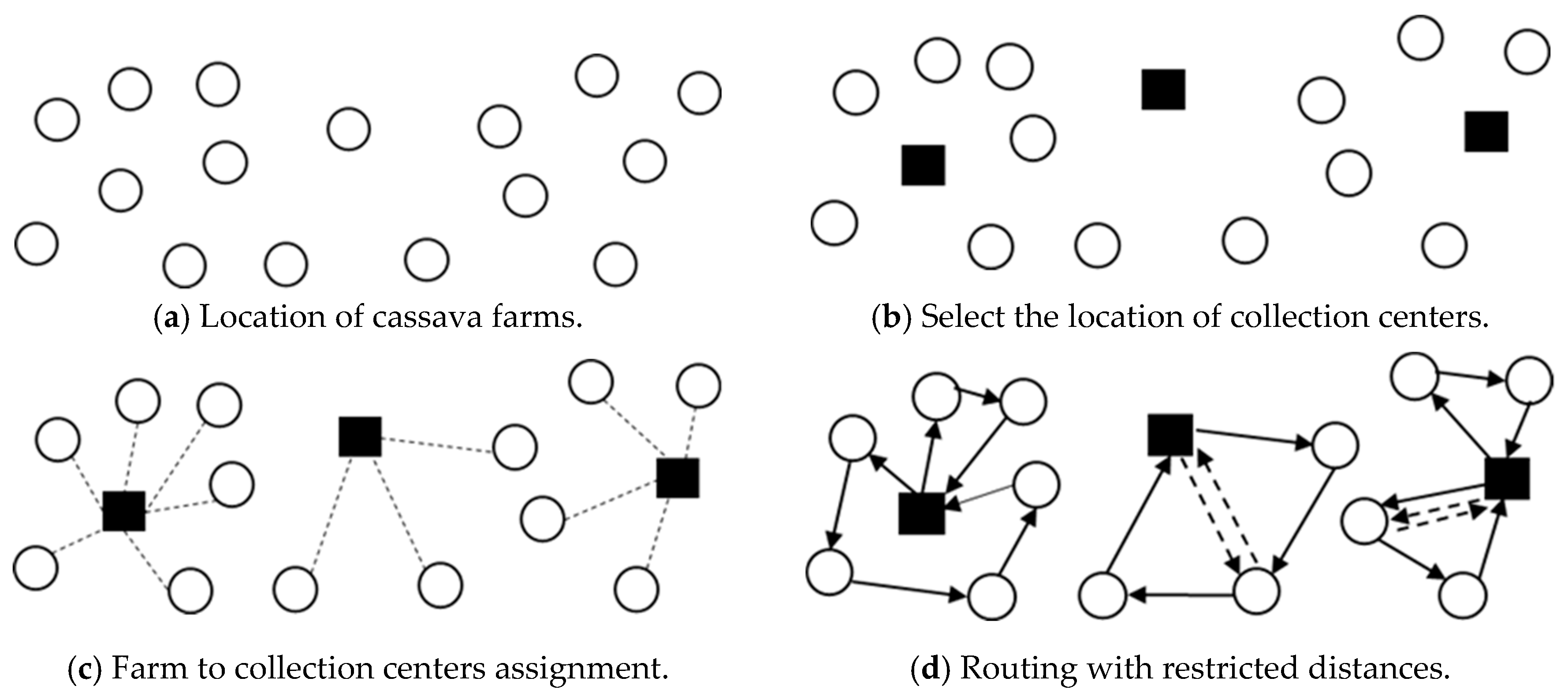
This research addresses the electric vehicle location routing problem (EVLRP) where EVs have a restricted distance of travel. The purpose of the case study is to decide upon a suitable location among candidate cassava farms, then open relevant collection centers (depots). After that, the cassava farms are assigned to relevant collection centers. Finally, transportation routes are prepared with restricted distances. These centers will gather cassavas from farms before sending them to cassava flour factories, the limitation of this research focuses only on activity between collection centers and farms. The transportation routes are provided for transferring cassavas from farm to collection center while the minimum of total cost is being considered. The model combined approach plans location and routing decisions simultaneously as they appeared in the literature surveys survey of recent research on LRPs [
40]. The EVs are used in transportation, where they start each route at the collection center with a fully charged battery.
Figure 1 illustrates the problem description. A partial shipment will be allowed if the farm has more cassavas than a vehicle’s capacity, as displayed by the dashed line in
Figure 1. The rest quantity after partial shipment will be transported once by routing at that farm.
The problem contains the following constraints which must be satisfied:
The total cassavas at farms assigned to a collection center must not exceed the capacity of the collection center.
Each farm must deliver all generated cassavas to a collection center.
Each route begins at a collection center and ends at the same place.
The total cassavas on EVs must not exceed their load capacity at any time.
Each farm can be visited more than once if the cassavas exceed a vehicle’s capacity. Then, partial deliveries are allowed.
The route range must not exceed a given distance.
Set
- I
set of cassava farms, I = {i1, i2, i3, …}
Parameters
- Sij
the shipment cost per kilometer from node i to node j
- Qi
cassava amount of farm i (kg)
- Dij
distance from node i to node j (km)
- V
EV load capacity (kg)
- Hj
collection center capacity (kg)
- Oj
opening cost if node j is selected to be collection center
- T
maximum distance available for each EV
- F
fixed cost per EV used. F is calculated by determining annual depreciation of EV divided by seasonal harvest period in one year (90 days). Then, the daily fixed cost per EV used is obtained.
Decision Variables
- yij
= 1 if farm i is allocated to collection center j and a partial shipment is needed
= 0 otherwise
- xij
= 1 if there is a transportation from farm i to farm j and the remain from partial shipment is routed
= 0 otherwise
- zj
= 1 if collection center j is chosen
= 0 otherwise
- ni
= number of partial shipments at farm i
- K
= number of EVs used
Support Variables
- ui
cumulative cassava quantity in EV at farm i, used for sub-tour prevention
- mj
number of round transports using for routing at collection center j
- ri
remaining cassavas after partial shipment from farm i
- ti
cumulative distance at farm i
Equation (1) is the objective function associated with the total cost minimization, which consists of four cost terms, i.e., the opening cost of collection centers, the transportation cost of partial shipments, the transportation cost of routing, and the fixed cost of using EVs. Equation (2) ensures that each farm has to be allocated to only one collection center. Equation (3) calculates the number of partial shipments and remaining cassavas in case the amount at that farm exceeds the EV load capacity. Equation (4) specifies that the capacity of each collection center must never be exceeded. Equation (5) decides the route of the cassava collection from the farm. In the case of zj = 0, only one arc can be 1, otherwise, mj arcs are going into the depot j. Equation (6) is the connectivity equation which ensures that the vehicle must leave farm i after it has been visited. Equation (7) determines the route among the farms that are allocated to the same collection center. Equations (8) and (9) guarantee that the route length must not exceed the maximum distance allowed for each EV. Equations (10) and (11) specify that the load capacity of each EV must never be exceeded and deal with sub-tour prevention, respectively. Equation (12) limit the number of EVs used. Finally, Equation (13) defines the domain of decision variables.
Obviously, the LRP considers to NP-hard combinatorial problems as it combines two NP-hard problems: the facility location problem (FLP) and the vehicle routing problem (VRP). Due to the complexity of the problem, the exact method proposed in early studies was limited by depending on a mathematical programming formulation. The authors usually use the reformulation and relaxation of some constraints such as sub-tour elimination and integrity [
41,
42,
43,
44]. Because of the exponential number of variables in the problem size, exact methods have been limited to a small and medium-sized instance with 20 to 50 customers [
45]. Based on our extensive study, the processing time was intolerable, and the model was frequently unsuccessful even though reformulations of constraints were attempted. For this reason, metaheuristics are usually used for solving realistic LRP problem size in more recent literature as we have reviewed in
Section 2. Moreover, we aim to provide the optimization system for future research to support stochastic supply according to daily product quantity. The selection of depots and routes may be dynamic moved based on the changing of daily product quantity. Metaheuristics algorithm seems to be more advantageous to obtain a suitable solution in a short decision time. Thus, an ALNS was developed to reach close optimal results for solving large-sized problems, especially concerning the case study problem.
4. Methodology
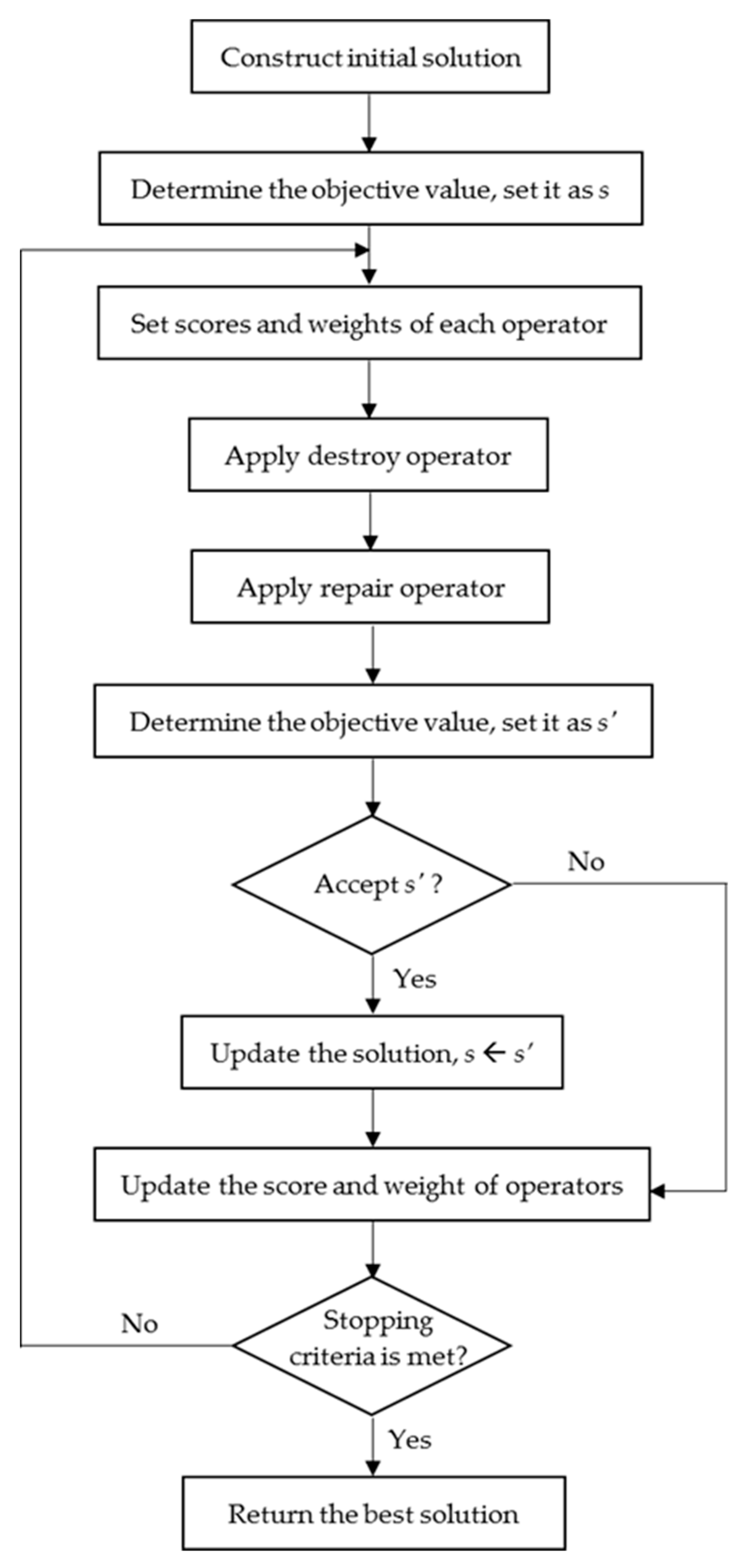
When the problem size increases, it is too complex to be solved by the exact method, i.e., via the Lingo software package. In this research, an adaptive large neighborhood search (ALNS) algorithm was developed for solving the EVLRP. The basic concept of an ALNS algorithm is repeatedly applying several destroy and repair heuristics to gradually refine solutions at each iteration. A pair of heuristic methods is randomly selected to improve the solution. The method is adaptive because the probabilities of selecting them are adapted based on their past performance. Generally, ALNS algorithms begin with the generation of an initial solution, then destroy and repair methods are selected to improve the solution. Let D be the set of destroy operators, D = {d1, d2, d3, …, di}, and R be the set of repair operator, R = {r1, r2, r3, …, ri}. Each operator owns initial equal weights at the first iteration, indicated by w(ri) and w(di). At every iteration, the weights are automatically adjusted until complete pmax iterations. The operator that has successfully improved solutions has a higher weight, so it has a higher probability to be repeatedly selected. The proposed ALNS used to solve the EVLRP is presented in
Figure 2.
4.1. Construct Initial Solution
The initial feasible solution is fabricated by the below procedures:
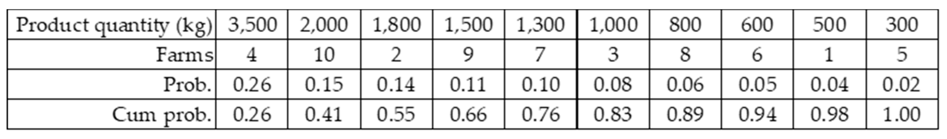
Step 1: Ranking the farms as the cassava quantity by descending order, then determining the probability of each farm based on the quantity. Due to the cumulative probability being directly varied based on the amount of the rubber, the farm that has more cassava would therefore have a higher chance of being selected, as shown in
Figure 3;
Step 2: Apply roulette wheel selection by choosing the random number between 0 and 1, then select a farm where the cumulative probability matches the random number. For example, if the random number is 0.18, farm 4 will be the depot;
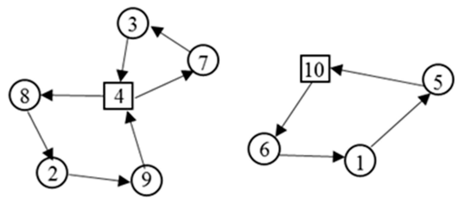
Step 3: Assign a farm to the opened depot by employing the nearest insertion method while considering the satisfaction of all constraints, such as the depot capacity, EV load capacity, and limited travel distance of EVs. If the load capacity and limited travel distance of EVs are satisfied while the depot capacity remains, terminate this route and start a new route to the same depot;
Step 4: If there are unassigned farms left, return to step 1–3 to open a new depot and assign farms to the depot again until there are no more farms left. An example of this initial solution is shown in
Figure 4, where farms 4 and 10 are established to be depots.
Step 5: Repeat steps 1–4 for 10 times to obtain different 10 initial solutions. Determine the objective value then select the best one.
4.2. Destructive Degree
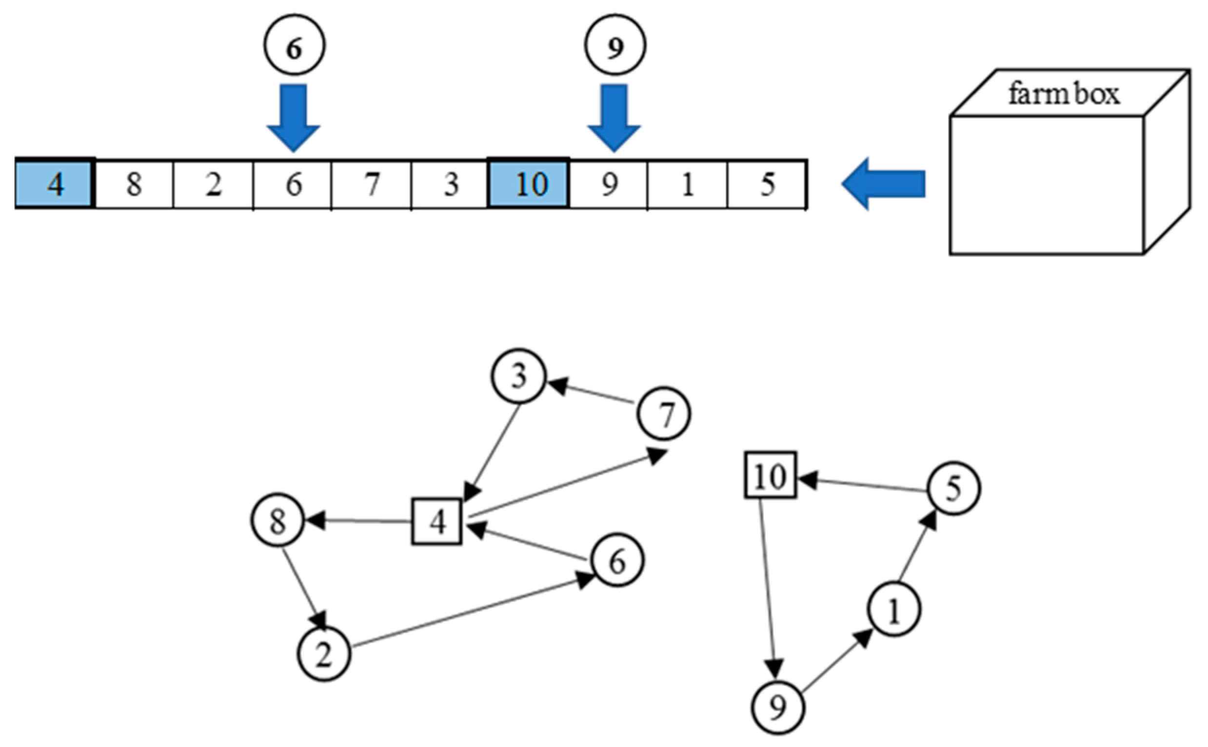
The destructive degree (dd) is the proportion of destruction that is applied to the incumbent solution. This work designed a specific set of destructive degrees as follows: dd = {10%, 15%, 20%, 25%, 30%, 35%, 40%}. At each iteration, the destroy operators will randomly select the destructive degree before execution. For instance, the current solution consists of 20 farms and the destructive degree is equal to 15%, so three farms (20 × 0.15) will be removed from the incumbent solution. Here, q is denoted as the removal farms. In this case, q = 3 will be put into the farm box waiting for the repair method operation.
4.3. Destroy Operators
This work designed five destruction methods for destroying the incumbent solution. These operators are used so that the searching area is continuously moving, thus a new solution is discovered. The different destroy operators are defined below.
4.3.1. Random Elimination
This is uncomplicated and fast heuristic. The basic concept is to randomly remove q farms and eliminate them from the current solution, as explained below. An example of random removal is displayed in
Figure 5.
Step 1: Randomly choose a destructive degree (dd);
Step 2: Randomly choose a number of farms (q) associated with dd from the incumbent solution;
Step 3: Detach q farms from the incumbent solution to the farm box.
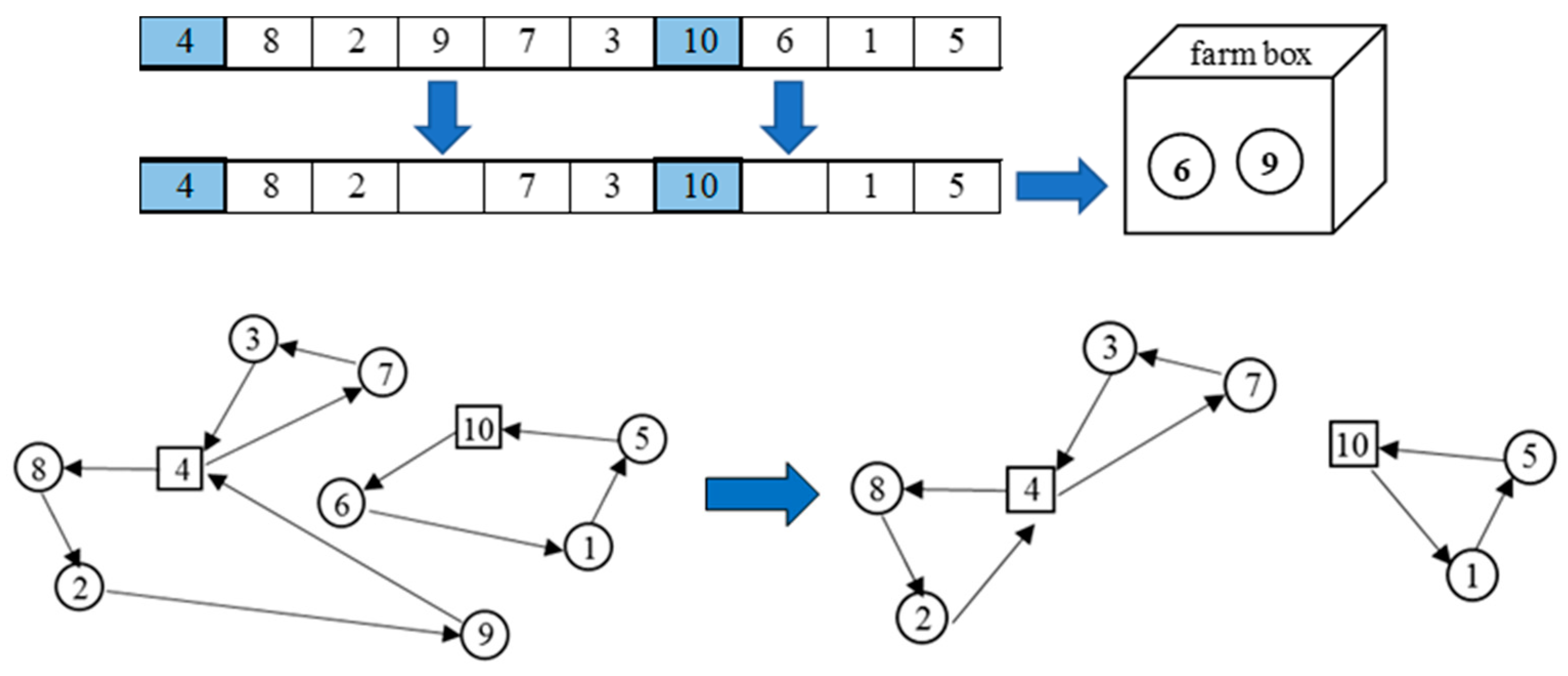
4.3.2. Worst Elimination
This operator eliminates q farms with the worst gain. Normally, the gain is the difference between the objective value when a farm is in the solution and the objective value when a said farm is eliminated.
Step 1: Randomly select a destructive degree (dd). If there are 10 farms and dd = 20%, then two farms will be detached (q = 2);
Step 2: Compute the objective value of the current solution;
Step 3: Re-compute the objective value excluding a farm one by one, then determine the different cost by comparing to the objective value in step 2. These different values are gains, whereas if there are 10 farms, there are 10 gain values;
Step 4: Sort farms in a decreasing order depending on the gain values from step 2;
Step 5: Detach the first two farms that own high gain values to the farm box.
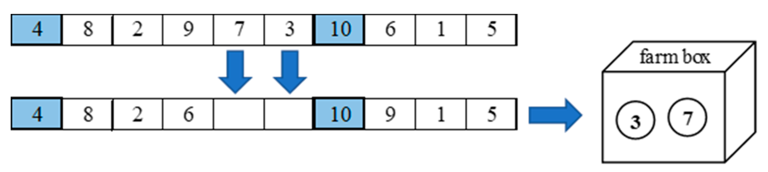
4.3.3. Connected Elimination
The connected elimination operator involves destroying farms that depend on the position of an adjacent point that is connected to the position of a removed point. This operator is similar to the related visits used by Shaw (1998) [
46], however, while Shaw selects a set of customers that are most related to each other respect to the distance, we apply a simple concept to move q-1 farms which are the closest to the stone farm.
Let the current solution contain 10 farms.
Step 1: Randomly select the destructive degree (dd). Let dd = 20%, where two farms will then be detached (q = 2).
Step 2: Randomly select a farm that will be removed and call this a stone farm.
Step 3: Determine the distance of each farm when travelling from the stone farm.
Step 4: Sort the farms in a descending order depending on the distances found in step 3.
Step 5: Eliminate q-1 farms that are located closest to the stone farm then put them into the farm box.
Figure 6 illustrates the connected removal when farm 3 is a stone farm and farm 7 is the closest location. Thus, these farms were removed from the solution.
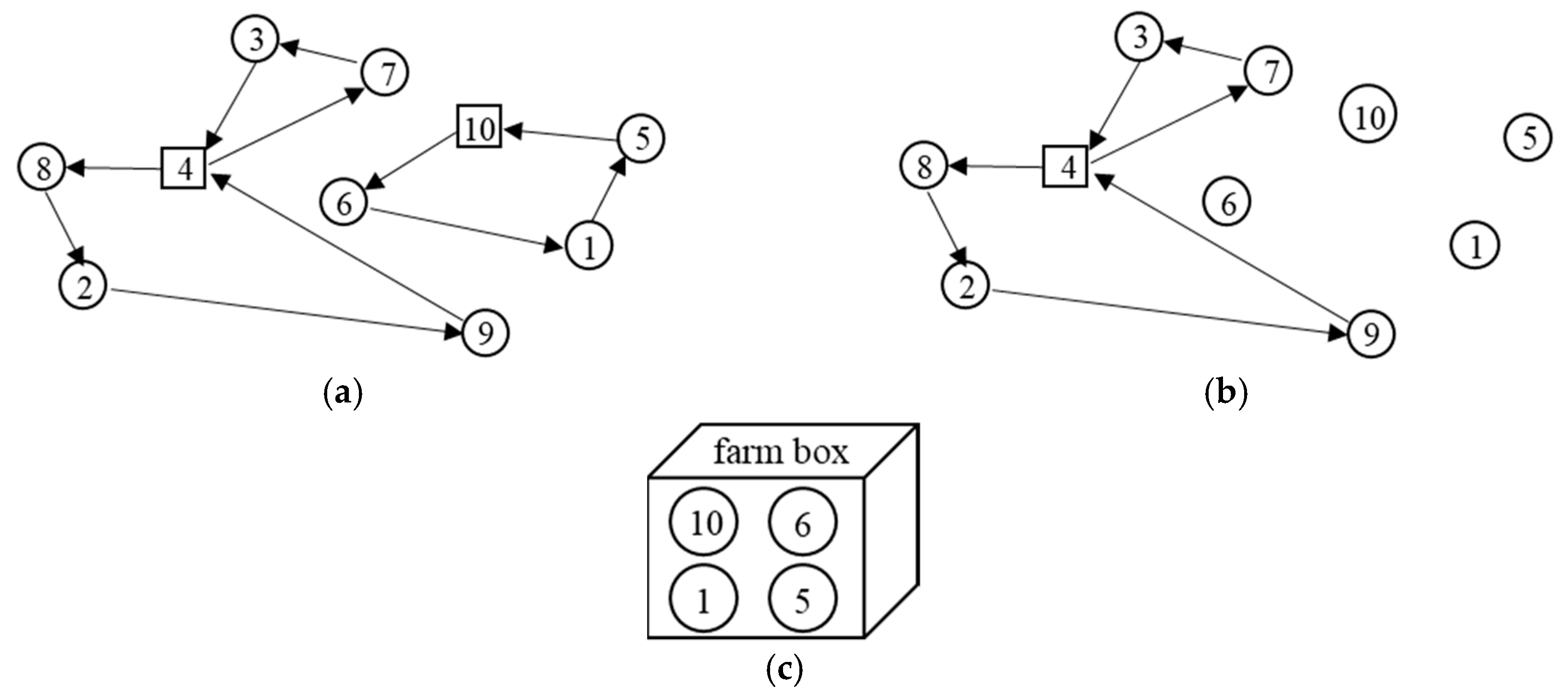
4.3.4. Depot Elimination
This operator has the purpose to increase the diversity of the searching area. The currently selected depot will be changed in its status from opened to closed, the current solution is shown in
Figure 7a.
Step 1: Randomly select one depot among all the opened depots, then close it. Let depot 10 be closed, as shown in
Figure 7b;
Step 2: All farms which are assigned to this depot are moved to the farm box, as shown in
Figure 7c.
Depot elimination allows the number of opened depots to change throughout the search, it will diversely impact the total cost in the objective function. After repair operation, the number of opened depots is possibly less or greater than the previous solution depends on the insertion method.
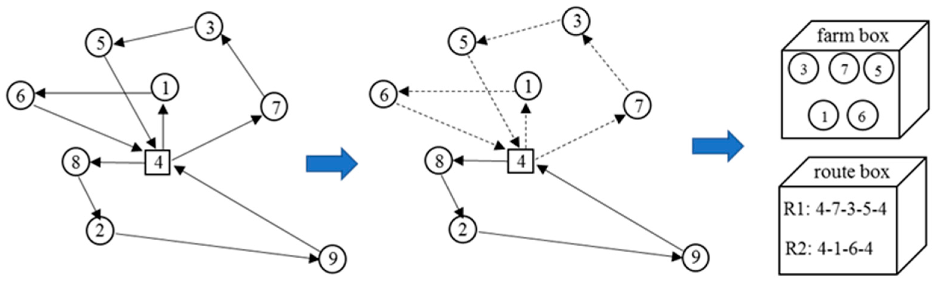
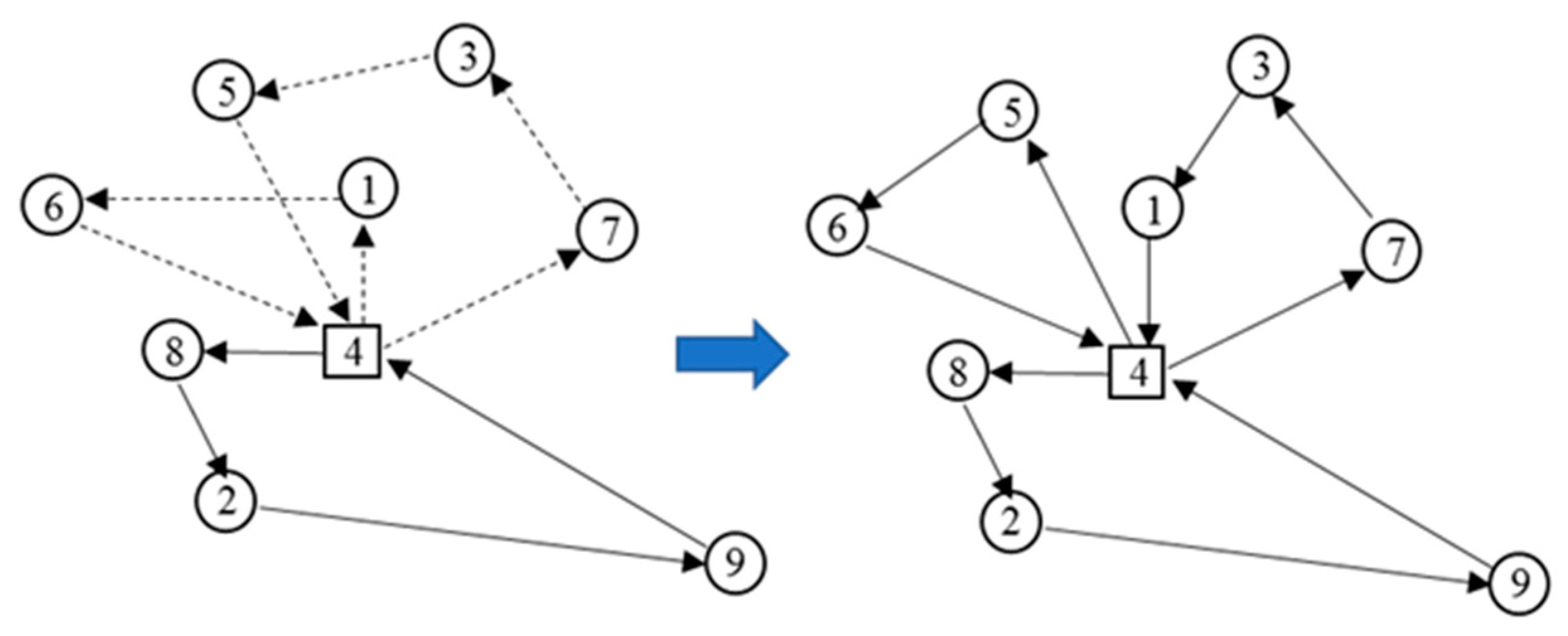
4.3.5. Route Elimination
The route elimination operator removes an entire route and moves the corresponding farms into the farm box. The new route will be rearranged by a repair operator. This method is a route improvement to explore better solutions.
Step 1: Randomly choose a random number of p, where 1 p 3;
Step 2: Then, p routes are chosen randomly from all routes. The selected routes and all corresponding farms will be removed to the route box and the farm box, as shown in
Figure 8 for
p = 2.
This operator stems from the idea that farms which are close to other depots may be more advantageous for reassignment in the current situation
4.4. Repair Operators
After the current solution is eradicated by the destroy operators it becomes an incomplete solution. A repair operator is used to improve the solution by reinserting the farms from the box back into the solution, where it will then be a complete solution. Four different repair operators were designed and are detailed below.
4.4.1. Random Repairing
The random repair operator is the most simple and uncomplicated method. The idea is to increase diversity by re-inserting the removed farms into any random position. The farms from the box are inserted randomly at any order and any position, as shown in
Figure 9.
4.4.2. Greedy Repairing
The greedy repair operator will select the best position by considering the lowest cost. This is important for intensification.
Step 1: Randomly select a farm in the box;
Step 2: Determine the objective value at each possible solution that this farm could be placed at;
Step 3: Place the farm at the cheapest position;
Step 4: Repeat the process until there are no farms left in the box.
4.4.3. Regret Repairing
The regret repair operator does not only take the minimal cost position into account but also the second-best. This was used to compensate for the characteristics of the greedy repair operator. The definition of the regret value is the different cost between the best position and the second best. Therefore, farms with a high regret value have to be inserted first. The regret repairing method used in this work is determined by Equation (13):
where
U is the set of currently unassigned farms and
is the cost of the insertion of farm i into the hth lowest position.
4.4.4. Route Repairing
The route repair operator is a local search methodology for improving the solution. This operator is only applicable to the route elimination operator. The operator randomly selects the removed route points in the route box, then the route point initiates a new route to improve the solution, as shown in
Figure 10. The new routes are expected to obtain a shorter path and reduce the travelling cost, which is the better solution.
If the route repair operator is selected after other destroy operators except for route elimination, the removed farms in the farm box will be reinserted according to the procedure of those operators.
4.5. Weight Adjustment and Solution Acceptance Methods
The selection of destroy and repair operators depends on their success in former iterations. Adjusting the weights of the operators is imperative to enhancing the possibility that successful operators are selected more frequently than less successful operators. At the first iteration, every operator is set to equal weight, then operators are weighted and selected independently. Every time an operator finds a new solution, reward () is added to the current score to obtain the new score. The weight at each iteration will be updated according to this score. The reward () is assigned as follows:
() = 10 if the operator finds a new global best solution;
() = 8 if the operator finds a solution that is better than the incumbent solution;
() = 6 if the operator finds a solution that is worse than the incumbent solution, but it is accepted by the acceptance method;
() = 2 if the operator finds a solution that is worse than the incumbent solution and it is also rejected by the acceptance method.
The acceptance method of ALNS is used to decide after the destroy and repair operations of whether to move forward with the incumbent solution (s) or with the new solution (s’). There are different strategies for implementing the acceptance method. Normally, an ALNS algorithm automatically accepts the better solution, but in the case of a worse solution, it must be judged by some techniques. However, this research proposes four acceptance methods, which are listed below.
- (1)
Greedy Acceptance (GA)
The solution s’ is only accepted if it is better than the incumbent solutions.
- (2)
Simulated Annealing (SA)
This method is motivated by a well-known metaheuristic, simulated annealing, which was first introduced by Metropolis et al. (1953) [
47]. SA is the most widespread acceptance method used by ALNS algorithms. Every improving solution is accepted. Nevertheless, if Z(s’) > Z(s), s’ is accepted with a probability, as shown by Equation (14):
where T is the temperature at the current iteration. T is decreased at every iteration by factor k.
- (3)
Threshold Acceptance (TA)
The new solution s’ is accepted if Z(s’) – Z(s) < Th. Th is called the threshold, which is decreased at every iteration by factor α.
- (4)
Old Bachelor Acceptance (OBA)
The new solutions’ is accepted if Z Z(s’) − Z(s) < Th with a threshold Th, which is the same as in the TA method. Th is decreased by factor α if a new solution is accepted. On the contrary, Th is increased by factor β if a new solution is rejected.
The decreasing factor α and increasing factor β were set by the intervals of [0.9, 0.9999] and [1.000, 1.1], respectively.
5. Computational Results
The proposed ALNS algorithm was coded in Visual Studio 2019 with the mathematical model prepared by Lingo version 11 on a laptop with an Intel Core i5-4210U 2.70 GHz CPU with 6 GB of RAM. The experimental framework was a comparison between solutions obtained by the ALNS algorithm and solutions provided by the Lingo software. The three groups of test instances were generated randomly using a uniform distribution. All instances contained distinct numbers of farms, vehicle load capacities, and collection center capacities. Details of the test instances are shown in
Table 1. The stopping criterion was set depending on the instance size. For small problems, the reported computational time was the duration after which the optimal solution was found. For medium, large, and case study problems, the algorithms were set equivalently to execute 1000 iterations for each run. The algorithms were executed three times, then they reported the best results among the three executions. Since the optimal solution was not obtained during the acceptable processing time for the medium, large, and case study problems, the processing time for Lingo was set to be 72 h for the medium problem and 120 h for the large and case study problems. The best solution and lower bound obtained by Lingo were presented and compared with the solutions that were obtained by the proposed algorithms. The MINITAB
® version 19 software package was used for statistical tests, where the significance level was set to be equivalent to 0.05 for all tests.
Since four acceptance methods have been embedded in the algorithm, the mixtures of the proposed ALNS algorithms are clarified in
Table 2.
The experimental results were reported in terms of their quality and time by being separately considered for each instance size. For small-sized instances, both Lingo and all proposed ALNS algorithms could generate optimal solutions in a short amount of CPU time, as indicated in
Table A1 in
Appendix A. This table reveals the time for which the proposed ALNS algorithm explores the solution.
As shown in
Table A2, the results obtained by Lingo are the best solution within the limited computational time that was set to 4320 min. The proposed heuristics can find beyond Lingo, where they generate better solutions while only requiring 2.45 min on average, which is 99.94% ((4320 − 2.45)/4320) less than Lingo. This means the proposed heuristics are effective for the medium-sized instance. Wilcoxon’s signed-rank test for matching pairs of data was performed to reveal whether the proposed ALNS algorithms were significantly different from the solutions obtained by Lingo. If
p-value from the statistical test is lower than 0.05, it can be concluded that a pair of data is significantly different from each other. The results from MINITAB
® are shown in
Table 3. In this table, the numbers are
p-values from the test. The signs
, =, and
specify that the solution is less than, equal to, or greater than the compared method.
The results in
Table 3 show that Lingo initiates worse solutions than all the proposed ALNS algorithms. Comparing the proposed heuristics, ALNS-1 and ALNS-3 are not different from each other as well as ALNS-2 and ALNS-4, but ALN-3 is worse than ALNS-4. From this result, it can be concluded that ALNS-2 and ALNS-4 outperform the other proposed heuristics for this instance size.
The experimental results of the large-sized instance (including the case study problem) are shown in
Table A3. Lingo could only find lower bound solutions within the limited computational time, which was set to 7200 min. However, the proposed ALNS took only 7.48 min on average, which is 99.89% ((7200 − 7.48)/7200) less than that of Lingo. Comparing the proposed heuristics, it seems that ALNS-4 is the most effective algorithm because it generates the lowest cost in the large-sized instance and case study.
The statistical test results found using Wilcoxon‘s signed-rank test for matching pairs of data via MINITAB
® are shown in
Table 4. The results are used to examine if the proposed heuristics are different than those of compared methods. The results show that the lower bound solutions from Lingo are lower than the solutions from all proposed heuristics, however they take a long computational time. Comparing the proposed heuristics, ALNS-1 is worse than ALNS-2 and ALNS-4. The best algorithm here, similar to the medium-sized instance, is ALNS-4.
To verify the effectiveness of the proposed ALNS algorithm, the percentage differences (
%dif) of the solutions generated by the ALNS were compared with the solution from Lingo. The percentage differences were calculated by Equation (15) and the results for all instance sizes are shown in
Table 5.
where
is the solution generated by the proposed ALNS algorithm and
is the solution generated by Lingo.
From the results of the medium-size problem in
Table 5, all the proposed heuristics obtain a better solution than Lingo, which only has the best solution within a limited amount of time. ALNS-4 is the most improved solution, generating 3.95% less time than the solution from Lingo. For the large and case study problems, Lingo obtains solutions lower than the proposed heuristics, but these solutions are only lower bounds, even at 120 h. The proposed heuristics generate a percentage difference of approximately 6% to 7% when compared to the lower bound. ALNS-4 obtains the lowest percentage difference from the lower bound, which is only 6.59%. The full results are shown in
Table A4.
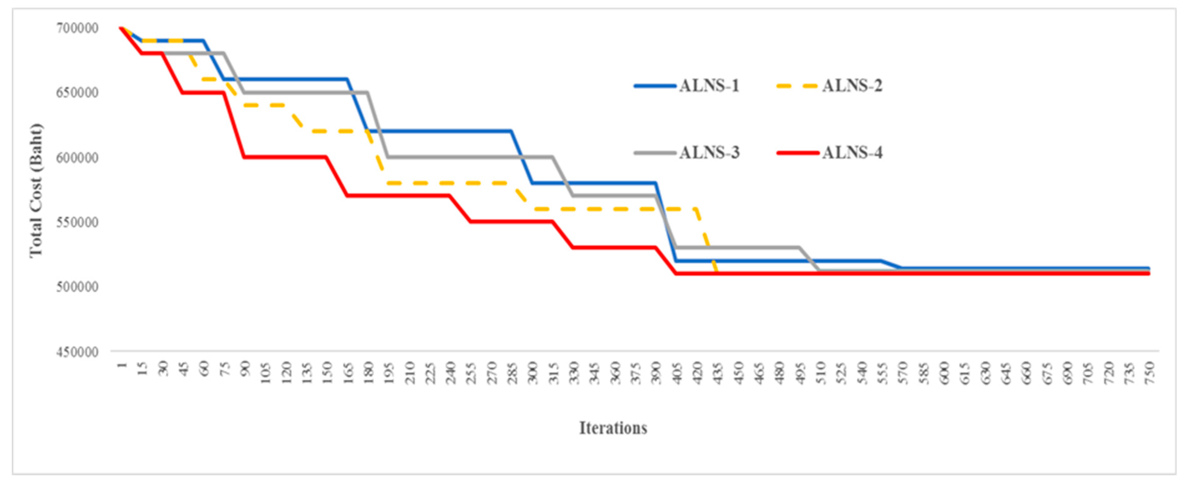
When comparing all the proposed ALNS algorithms, an experiment was performed to study the behaviors of the proposed methods when searching for the best solution. The proposed algorithms were run for a long duration to solve the case study problem until reaching mutual states. The best solutions obtained from each algorithm were recorded and the simulation plots are shown in
Figure 11. All methods started at almost the same solution level, but ALNS-1 slowly approached the best solution. The algorithm did not frequently move enough to escape from local optima, so it was difficult to discover the new best solution. The turning point of the line implies a change in the search area. On the other hand, ALNS-4 improved its best solution faster than the others, where it then moved to be the best until the end. Besides, ALNS-4 frequently changed the searching area, where it could escape from local optima. ALNS-4 was applied with an adaptive threshold to accept a new solution, where the threshold was periodically adjusted at each iteration. This was important for the concept of diversification, which let the algorithm always move to other searching areas.
Our proposed method has been tested on the well-known set of instances for the LRP that was gathered by Barreto (2007) [
48].
Table 6 provides the information of Barreto’s instances and a comparison of the solutions obtained by other methods from the literatures and our proposed ALNS-4. Column 1 shows the instance name that implies the number of customers and the number of candidate depots. Columns 2–3 show the vehicle capacity, the best-known solutions (BSK) reported by previous literature. The solutions obtained by multiple ant colony optimizations (MACO) [
49] and ALNS [
50] are shown in columns 4–7. Columns 8–9 show the solutions obtained by the proposed ALNS-4. It includes the percentage deviation (%dev) to compare the performance in each method. The %dev is calculated by dividing the difference between the solution values from the method by the values of the best-known solutions. Bold numbers identify that best-known solution values are obtained by the proposed algorithm.
It can be observed that the ALNS-4 is competitive with ALNS, because its average deviation to the ALNS is +0.02% (0.18% − 0.16%) concerning to the BKS. However, ALNS-4 has achieved 8 of 13 BKSs, while the percentage of finding BKS is only 61.54%, which is slightly lower than ALNS (76.92%). ALNS-4 has obtained more average deviation than the MACO around +0.05% (0.18% − 0.13%). Nevertheless, the MACO can achieve only 8 of 13 BKSs (57.14%), which is lower than the ALNS-4.
Finally, the best solution of the case study problem was obtained by applying ALNS-4 to the problem.
Table 7 shows the computational results of solving the case study problem. It was found that the location and transportation routes were managed efficiently by the proposed heuristic. From all 86 cassava farms, eight farms were selected to be collection centers. Overall, 31 routes were provided to collect the products from all farms while considering the restricted driving range of EVs, which was set to 600 km in this case. Correspondence from Liimatainen et al. (2019) [
51], the specification of the Tesla electric truck model “Semi” indicates the driving range of 480 to 800 km. Thus, we refer to this specification for determining the constrained distance in our case. The total cost was minimized to 509,906 baht. Consequently, it can be concluded that the proposed ALNS solution is a powerful method that can minimize the total cost in the agriculture sector by using EVs for transportation.
6. Conclusions and Future Works
This research studies the electric vehicle location routing problem (EVLRP), which considers the use of electric vehicles with restricted driving ranges in the agriculture sector to minimize the total operational cost. The operation of electric vehicles is becoming attractive in the logistics sector since they reduce environmental impacts caused by transportation activities. To the best of the author’s knowledge, this is the first time that this idea has been applied to a realistic agricultural problem. A mixed-integer programming model was formulated and solved by the exact method software package Lingo. The software could only handle small-sized problems and it could not deal with medium and large-sized problems, especially the case study problem. Thus, an ALNS algorithm was proposed for solving the EVLRP.
In this paper, the ALNS was developed by deploying destroy and repair concepts. The proposed ALNS consists of five destroy and four repair operators. These operators were selected randomly to develop solutions in each iteration. Moreover, four acceptance criterions were applied, and four sub-heuristics were created to assess the effectiveness of the solution acceptance method. The computational results show that ALNS-4 with the old bachelor acceptance method outperforms all the other proposed ALNS methods. Therefore, ALNS-4 was deployed to solve the cassava location routing problem in Thailand. Then, eight collection centers and 31 routes were established with the lowest overall operational cost. This result indicates that the proposed heuristic method can solve the problem effectively according to the EV travel distance constraint, as well as other constraints. Moreover, the proposed methodology can be applied to other related industries as well.
Nevertheless, there is still an opportunity to extend this paper. Future work would be to study adding time windows as well as heterogeneous fleets with various vehicle capacities and driving ranges. Furthermore, the maintenance cost and depreciation of EV batteries should be considered in the operational cost. The author believes this can be included to formulate a realistic model and will be a worthy extension. Additionally, although the proposed ALNS solution is very efficient and uses a well-known heuristic method, generating new destroy and repair operators with new acceptance methods will be valuable to study. Consequently, the solution approach of the problem should include hybrid metaheuristics to assess the efficiency of various methods for dealing with this kind of problem.


