1. Introduction
The permanent magnet synchronous motor has the advantages of simple structure, low loss, high power factor and high efficiency, so it has been widely used in the fields of industrial robots, aerospace and other fields. In order to achieve high-performance control, it is necessary to accurately detect the initial rotor position [
1,
2,
3,
4,
5,
6,
7,
8,
9]. The running performance of the motor will be decreased and a smooth start-up process will not be achieved unless the initial rotor position of the permanent magnet synchronous motor is accurate. Therefore, the initial position of the rotor needs to be accurately estimated in order to realize the high-performance control [
1,
2,
3,
4,
5,
6,
7,
8,
9].
There are two kinds of calculation principle in the position sensorless control of a permanent magnet synchronous motor (PMSM). The first one is based on the fundamental mathematical model of the PMSM and the second is based on the salient characteristics of the motor. Among the above-mentioned methods, the first method usually extracts the position signal from the back electromotive force (EMF), according to the relationship between back EMF and rotor position. The EMF can be obtained directly from the voltage equation. This method is very simple, but it needs accurate motor parameters [
10]. However, it is very difficult to calculate the back EMF based on the voltage equation because the back EMF of the motor will be small when the speed drops to zero. Therefore, it is necessary to make use of the salient polarity of the motor. In order to obtain significant salient polarity, the signal injection method is usually used to obtain the high-frequency response current, which contains the rotor position information. The high-frequency signal injection method is based on the salient pole effect of the motor, which can effectively estimate the initial rotor position of the permanent magnet synchronous motor. According to the nature of the injection signal, it can be divided into a rotating high-frequency signal injection method [
11] and a high-frequency pulse signal injection method [
12]; according to the position of the injection signal of the whole motor control system, it can be divided into a high-frequency voltage signal injection method [
12,
13,
14] and a high-frequency current signal injection method [
15]. Among these, the representative methods include a voltage pulse vector injection method [
16,
17] and a high-frequency signal injection method [
17,
18]. In reference [
19], a series of voltage pulses with equal amplitude and different directions are applied to the motor, and the initial position of the rotor is estimated by detecting and comparing the corresponding stator current, which is the basic idea of the voltage pulse injection method. The theoretical error of this method is small, but it is difficult to determine the pulse width and amplitude and to implement this approach, and the error also affects the accuracy of position estimation. In reference [
20], initial rotor position is estimated from a spatial saliency tracking estimator. Magnet polarity is identified simultaneously by using the fundamental harmonic of rotor position in the second harmonic frame of the carrier frequency due to d and q-axis saturation saliencies for both rotating and pulsating voltage carrier injection. However, this method uses a low-pass filter, and the algorithm is complex and difficult to implement. In reference [
21], the high-frequency square wave signal injection method is adopted. This method does not need to use a filter to extract the high-frequency response current, which increases the system bandwidth. However, the high-frequency square wave signal has the disadvantages of strong sensitivity to the measurement error, and is easily affected by the sampling delay and the nonlinear effect of the inverter. In reference [
22], according to the characteristics of the phase induction of Inner Permanent Magnet Synchronous Motors (IPMSMs), the corresponding relationship between the rotor position and the phase inductance is obtained. In this method, the rotor position information is obtained easily, with several basic math operations and logical comparisons of phase inductances, without any coordinate transformation or trigonometric function calculation. However, the algorithm is sensitive to disturbance and has poor robustness.
First of all, this paper studies the conventional high-frequency sinusoidal voltage injection method [
23,
24]. The principle of this method is to inject a high-frequency sinusoidal voltage signal into the α-β-axis, and then generate the high-frequency response current. Finally, the initial position of the rotor is obtained by using the relationship between the amplitude of the high-frequency response current and the position of the rotor. However, this method requires bandpass filters when demodulating the amplitude of the high-frequency response current, and the use of the filters will delay the rotor position and cause errors. When calculating the rotor position, the arcsine formula is used. This method includes physical quantities such as inductance and injection voltage. These physical quantities will affect the calculation results and make them inaccurate.
In this paper, aiming at the shortcomings of the traditional sinusoidal signal injection method to detect the initial position of the rotor, a new method based on a high-frequency sinusoidal voltage signal injection method is proposed. The advantages of the proposed method are as follows.
- (1)
There is no need to use a filter to extract the high-frequency response current.
- (2)
It is less dependent on parameters.
- (3)
The method is simple and effective, and occupies fewer resources of the digital control system.
Theoretical analysis and experimental results show that the method can accurately detect the rotor’s initial position, and verify the feasibility and effectiveness of the method proposed in this paper.
This paper discusses the effectiveness of this method based on the following aspects. First, the mathematical model of the method is deduced and the principles of the method are described. Second, the implementation steps of the method are introduced and error analysis is carried out. Next, the rotor polarity is judged. Finally, the effectiveness of the method is verified and conclusions are drawn through experiment.
3. Current Response to Calculate Rotor Position
3.1. Traditional Method of Angle Extraction
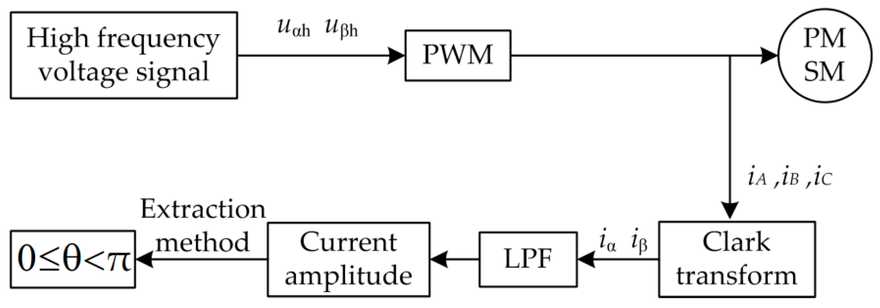
From the above section, after the high-frequency voltage signal is injected into the α-β-axis, the response current contains the initial rotor position information and
θ can be extracted from it, as shown in
Figure 3. The relation between the high-frequency response current and
θ is obtained by Equation (15).
In the Equation (14),
Iαβh contains the position information of the rotor. It is necessary to extract the high-frequency current component
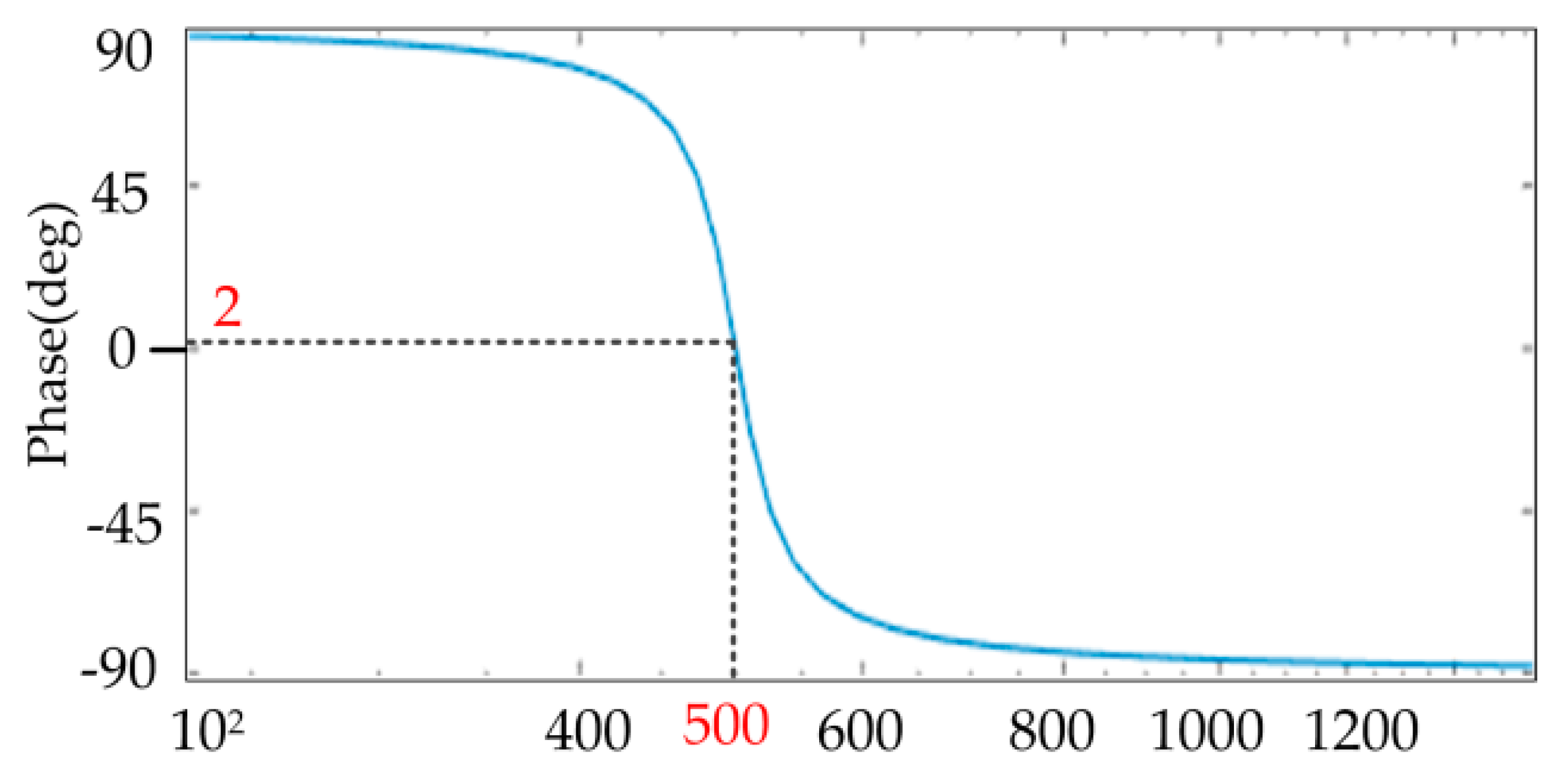
Iαβh with a low-pass filter (LPF) or bandpass filter (BPF). However, the use of the LPF or BPF will affect the accuracy of the estimation. For example, a high-frequency signal of 500 Hz is extracted by BPF. The type of BPF is a typical second-order bandpass filter and the cut-off frequency is 500. The phase-frequency characteristic curve of the BPF, designed according to the above requirements, is shown in
Figure 4.
From the phase-frequency characteristic curve, it can be seen that a high-frequency signal passing through the BPF produces a phase shift of about 2° at 500 Hz. This phase shift also changes as the order of the filter, the cut-off frequency, the passband bandwidth and the frequency of the injected high-frequency signal change. Therefore, the use of a bandpass filter causes a phase shift in the signal and a bias in the estimated angle, which is one of the main problems to be solved below.
3.2. Proposed Angle Extraction Method
As can be seen from the above section, after injecting the high-frequency voltage signal into the α-β-axis we can get the response current, and the amplitudes of the response current,
Iα and
Iβ, contain the information of the rotor position angle θ. The traditional method uses a low-pass filter to obtain the response current amplitudes
Iα and
Iβ, while the low-pass filter will cause a delay in the phase angle and cause errors. These errors also need a corresponding compensation algorithm, which increases the calculation amount of the system. Therefore, in order to reduce the errors caused by the use of the filter, the method of peak sampling is used; when sin
ωht = 1, the values of
iαh and
iβh are equal to
Iα and
Iβ, and the current amplitudes of
Iα and
Iβ are obtained from Equation (17). This method does not need to use a low-pass filter and avoids the generation of phase delay.
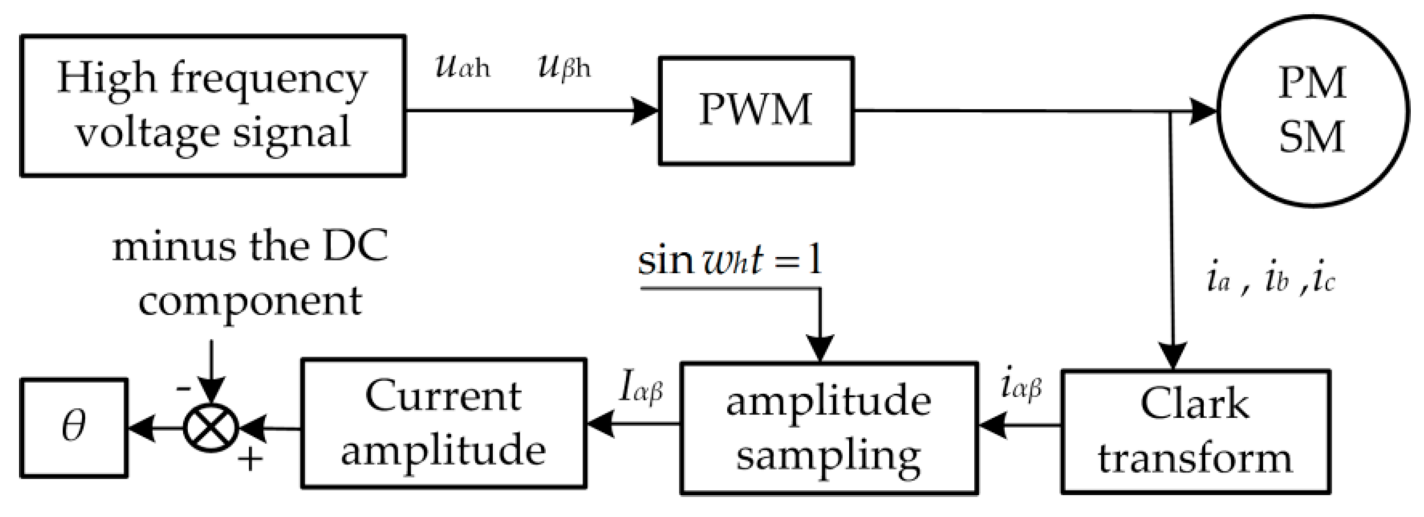
After
Iα and
Iβ are obtained, the DC component is subtracted, and a component that is only related to the position angle
θ can be obtained from Equation (15). The system block diagram is shown in
Figure 5.
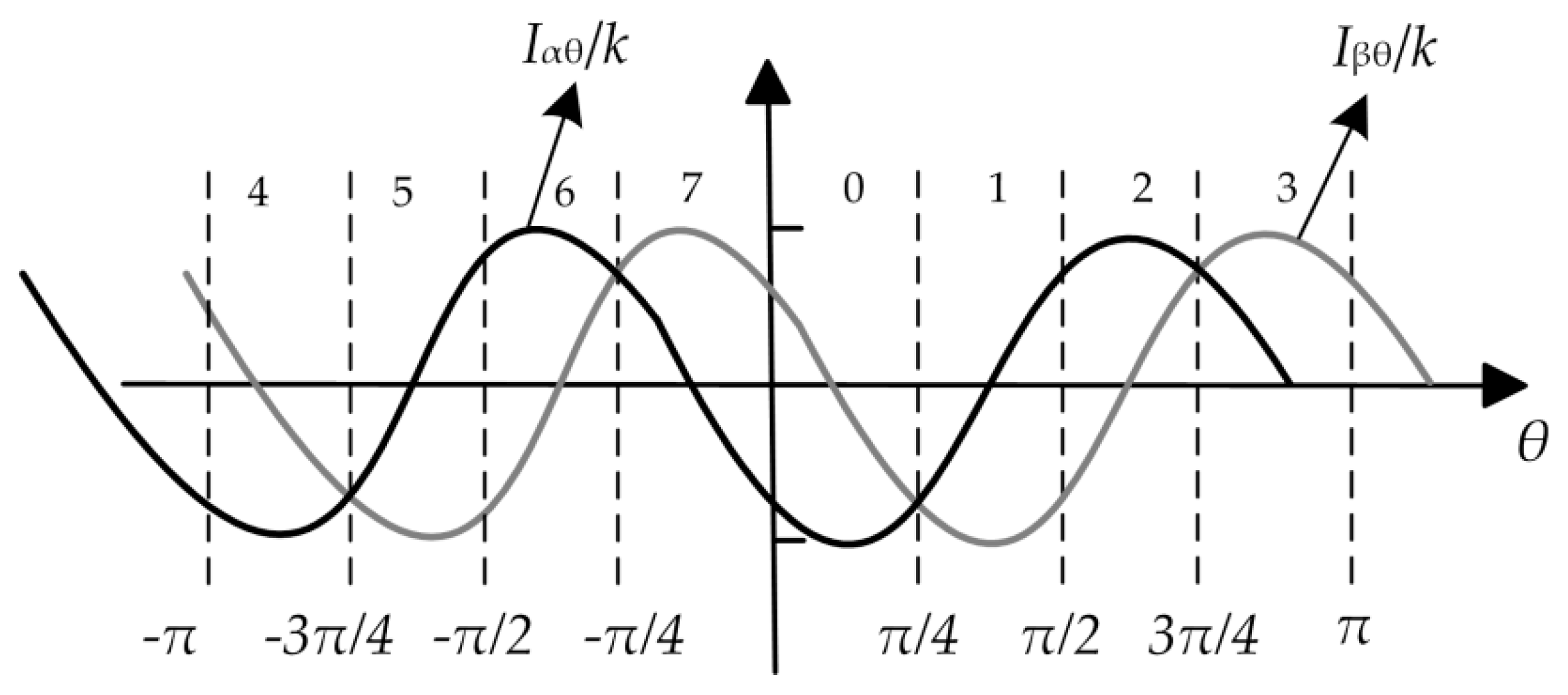
According to Equation (15), the relationship between high-frequency response current and
θ is shown in
Figure 6.
From Equation (15) and
Figure 6,
θ can be estimated through the following formula:
According to the size of
Iαθ and
Iβθ, the interval of
θ can be determined, and the formula can be used to estimate
θ by a look-up table method. For example,
θ can be estimated from the zero interval in
Figure 5.
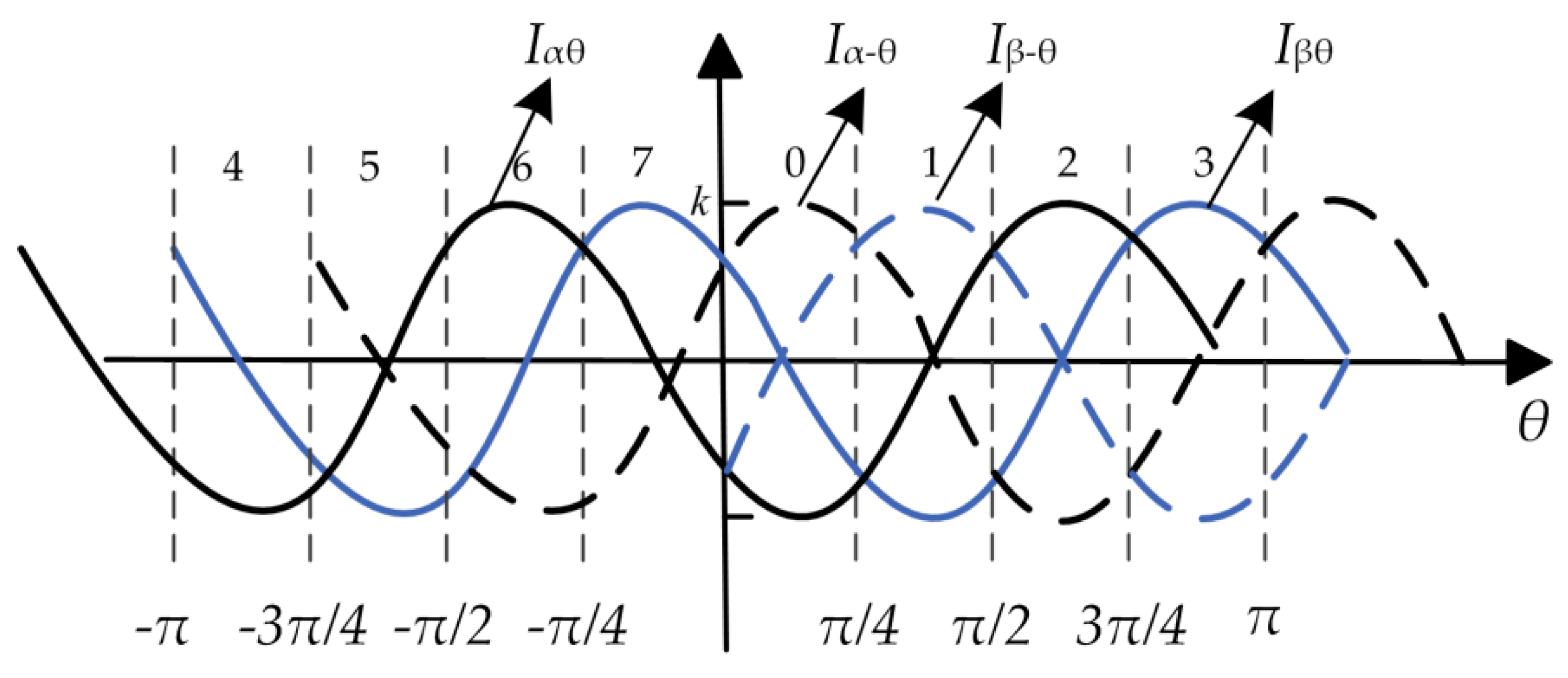
However, there are some inadequacies in the method of estimating θ according to the trigonometric function: since the k contains Um and ωh, the position angle estimation will be affected by these parameters. If the motor parameters are not accurate, then the calculated initial angle will also have errors. By Equation (15), Iβθ/Iαθ = -tan(2θ–π/4), and there is θ = [π+arctan(Iβθ/Iαθ)+π/4]/2. By using the arctan, the influence caused by the change of k value will be reduced, and the calculation of θ will be more accurate. At the same time, when Iβθ/Iαθ is infinitely large in a special position, it needs to be linearized, solved by the following linearization method and without k.
Figure 7 is obtained by inversion of
Iαθ and
Iβθ in
Figure 6. From
Figure 7, the relationship between the magnitude of the current response amplitude and the interval of
θ is given by
where
Iα-θ and
Iβ-θ are, respectively, the inverse of
Iαθ and
Iβθ, as shown in
Figure 7. The case of π<
θ<2π is same as that of 0<
θ<π, and the next section introduces the determination of the two cases. First, the interval of
θ is determined by Equation (19), and then
θ is calculated according to the arctan value. When the value of
Iβθ/
Iαθ between 0 and π is infinitely large, that is,
Iαθ is zero, then the corresponding
θ has two values, 3π/8 and 7π/8. Using the linearized formula, we can calculate the angle around the two values within 1 electrical angle, and the other values can be calculated by the inverse tangent method.
In the formula, the value of arctangent is taken between (–π/2, π/2), and the value of θ in the formula is within an electric angle of 3π/8 and 7π/8, which is calculated according to the following linearization formula.
The linearized calculation method can calculate the error angle, and this can be calculated as Equation (22).
We take the linearization formula near 3π/8 as an example, where
θ is the actual angle of the motor, and Equations (22) and (15) are combined to get the following formula
When θ = 3π/8, it is taken into the above formula, then the calculation error is less than 0.68 electric angles. This shows that the position angle obtained by the linear calculation method has minimal error and the effect of the error on the start-up of IPMSM can be ignored. At the same time, the error is produced only on small interval of θ in Equation (21), and has no effect on the other positions.
3.3. Angle Error Analysis
When the rotor position is at a special angle, the switching error analysis for the arctangent method and linear formula method is as follows.
According to
Section 3.1 and Equations (20) and (21), when the initial position of the motor is near a special angle, for example, 3π/8 and 7π/8, the switching between Equations (20) and (21) is required. When arctan (
Iβθ/
Iαθ) is less than 89° (electrical angle), the position angle is calculated by Equation (20). When arctan (
Iβθ/
Iαθ) is greater than 89° (electrical angle) and less than 91° (electrical angle), the position angle is calculated by Equation (21). When the formula is switched, the position angle will produce an error. For example, when
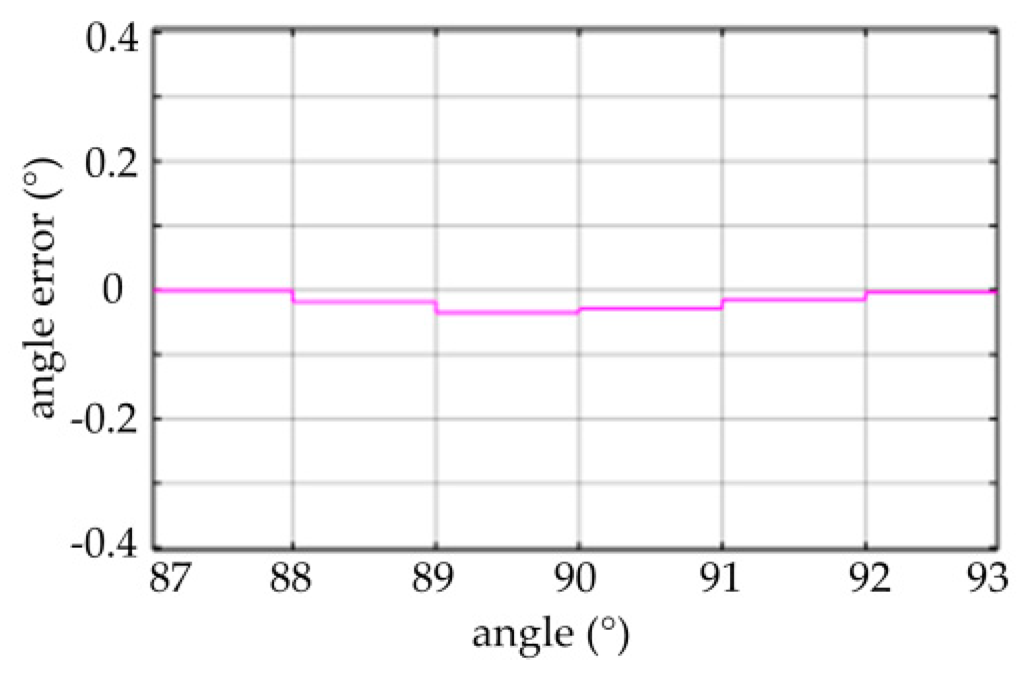
θ is 3π/8, the switching errors of Equations (20) and (21) can be expressed by Equation (23).
According to Equation (24), the angle error of formula switching is 0.1° (electrical angle), and the error of the above linear Equation (21) has been calculated before, so when Equations (20) and (21) are switched, the influence of angle calculation can be ignored. When
θ is 3π/8, the simulation diagram of angle error is shown in
Figure 8. It can be seen from the figure that the error brought by formula switching is less than 0.1° (electrical angle), which is not much different from the theoretical calculation. This shows that the influence of angle error brought by formula switching can be ignored.
The influence of Um is analyzed as follows.
As mentioned before, in the traditional method, arcsin (
Iβθ/
k) is used to calculate
θ in Equation (15). It can be seen that the Equation has coefficient
k, and
k contains physical quantities such as
Um. The high-frequency voltage contains high-order harmonic components, which will bring errors to the calculation results. According to Equation (16), we have
Based on the theoretical analysis of the influence of voltage Um, taking the 20 V high-frequency voltage as an example, The angle is calculated by using the arcsin formula and the formula is θ = [- arcsin (Iβθ/k)+π/4]/2. When θ = π/4, in combination with Equation (15), arcsin(−0.707) can be calculated. Then combining Equation (24), arcsin(−0.707)=arcsin(−14.14/20). The voltage contains high-order harmonics. Taking the third harmonic as an example, the amplitude of the third harmonic is Um3 = 20/3 V = 6.67 V. The sum of Um and Um3 is 26.67 V. Finally, the actual voltage injected into the α-β-axis will become 26.67 V, so value of arcsin will become arcsin(−14.14/26.67). After calculation, there is a 6.5° (electrical angle) deviation between θ and π/4, which has a great influence.
4. Polarity Judgment
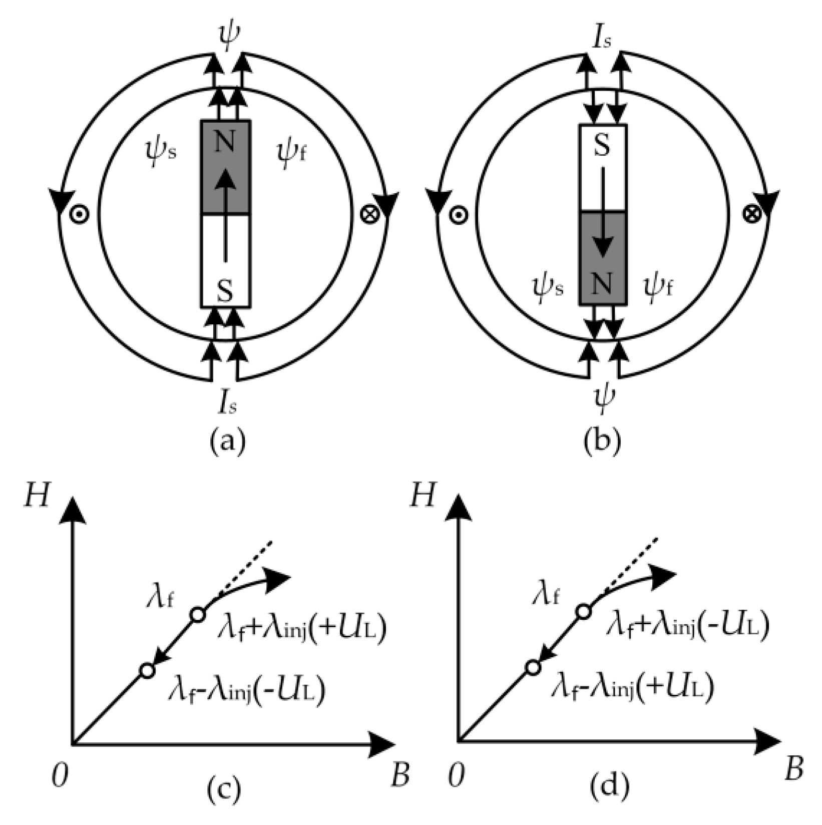
It can be seen from the above section that when extracting the rotor position information from the high-frequency current response signal, due to the symmetry of the rotor salient pole, only 0 to π can be estimated, and the actual positive direction of the d-axis cannot be determined; that is, the rotor polarity cannot be determined. Therefore, polarity judgment is needed. The principle of polarity judgment is that the stator current generates a magnetic field ψ
s, and the rotor permanent magnet generates ψ
f. When the two magnetic fields are in the same direction, this will have a magnetic aid effect on the synthetic magnetic field ψ of the air gap, as shown in
Figure 9a, increasing the magnetic saturation degree of the stator core, and entering the saturation area, as shown in
Figure 9c. As the magnetic resistance increases, the winding inductance will decrease, and the winding current and inductance increase. In contrast, the winding current will increase; when ψ
s and ψ
f are in opposite directions, demagnetization will occur, as shown in
Figure 9b, the magnetic saturation of the stator core will weaken and return to the linear area, as shown in
Figure 9d, the magnetoresistance will decrease, the magnetoresistance inductance will increase, and the winding current will decrease.
The method steps of polarity judgment are as follows.
- (1)
A position angle θ has been calculated in the previous section, and a constant voltage UL has been injected along the angle of θ. The d-axis will generate a response current in this period of time, and reach the peak value. Remember the current value is id,θ, and its absolute value is |id, θ|.
- (2)
Make UL = 0, and reduce the d-axis current to zero, so as to avoid affecting the following steps.
- (3)
Inject the voltage UL of the same amplitude and time along the direction of θ+π, record the peak value of d-axis response current as id,θ + π and record the absolute value as|id,θ + π|.
- (4)
Compare |id, θ| and |id,θ + π|, if |id, θ| > |id,θ + π|, then prove that θ is the direction of the N-pole and θ is the actual angle, otherwise, prove that θ is the direction of the S-pole and θ + π is actual angle.
When the rotor position angles are
θ and
θ + π, a voltage with amplitude
UL is injected into the d-axis
where
is the step variable with time and its maximum value is
UL. Since
RS is very small, it is not included, and Equation (26) can be reduced to
Equation (26) shows that when the step process is over,
is equal to
UL, and there is an inverse relationship between the maximum values of
id and
Ld. In this way, the amplitude of the current response is obtained by injecting the high-frequency voltage into the d-axis, then recording the d-axis current amplitudes, |
id,θ| and |
id,θ+π|, when the position angles are
θ and
θ+π respectively. It can be gained that
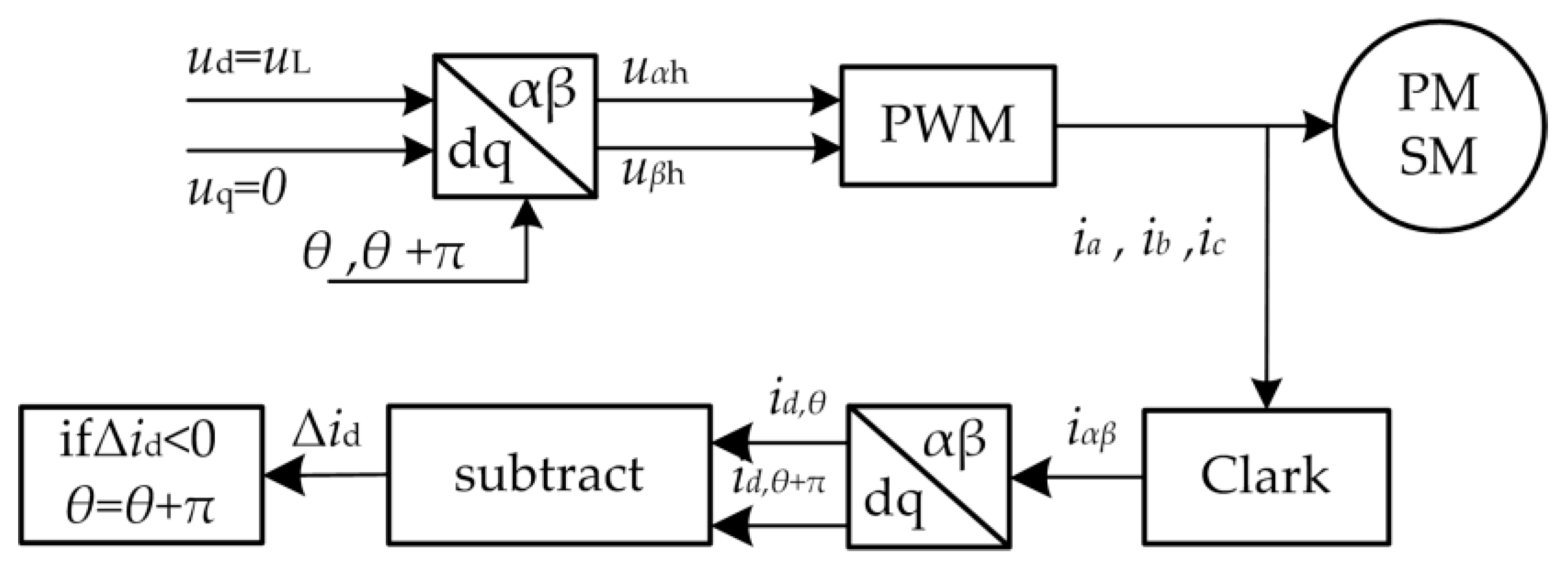
The system diagram of polarity judgment is shown in
Figure 10.
5. Experimental Results
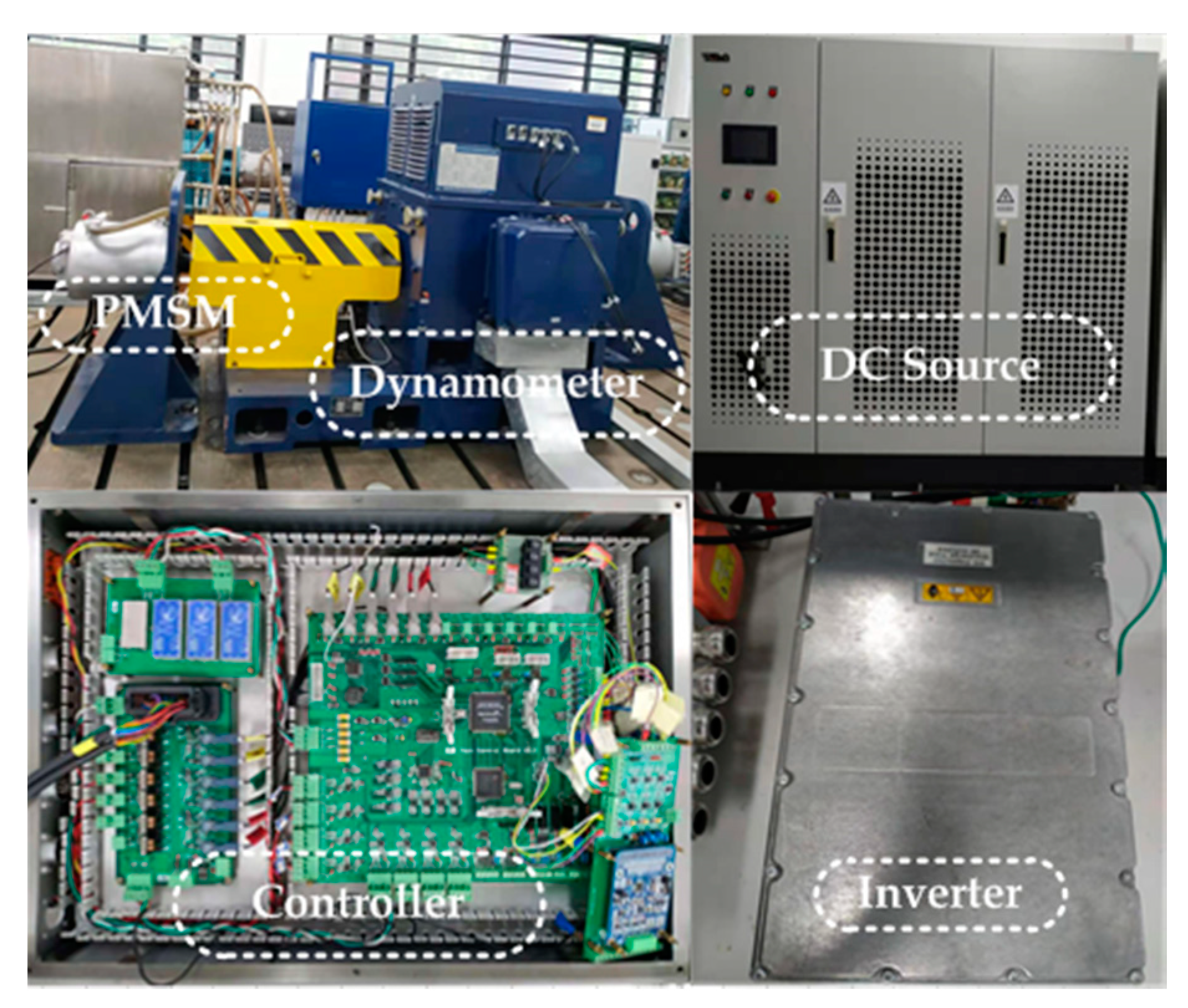
In this study, the theoretical correctness of the rotor initial position detection was verified by experiment. An experimental platform for detecting initial rotor position of permanent magnet synchronous motor was set up, as shown in
Figure 11. In the experimental system, an interior permanent magnet synchronous motor with a rated power of 20 kW was selected as the research object and the rotor had a salient pole structure. The parameters of the motor are shown in
Table 1. The core of the control system was a TMS320F28335, the main circuit was a voltage type three-phase inverter and the switching frequency was 10 kHz. The amplitude of high-frequency voltage injected into permanent magnet synchronous motor was 20 V, and the frequency was 500 Hz.
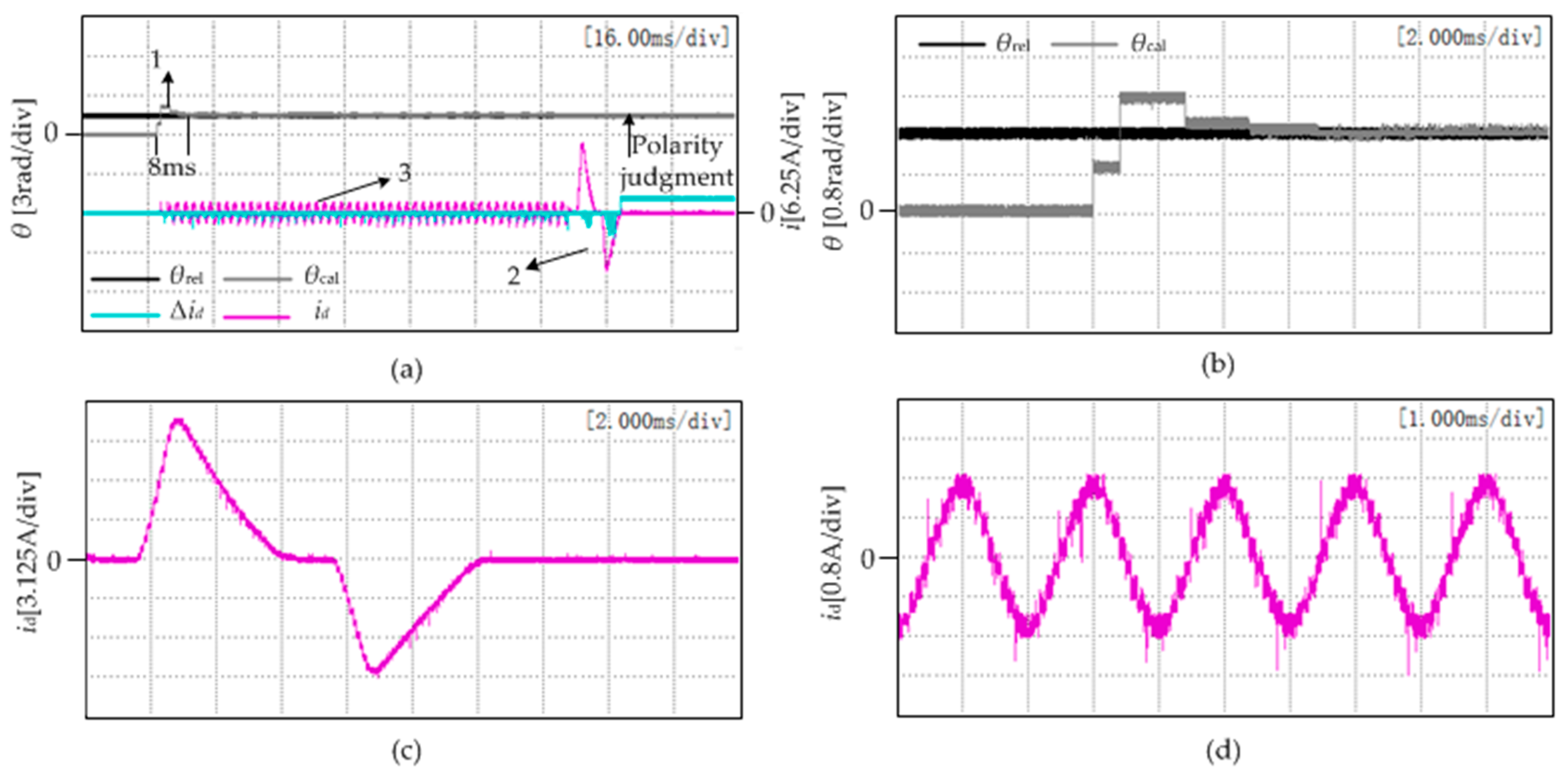
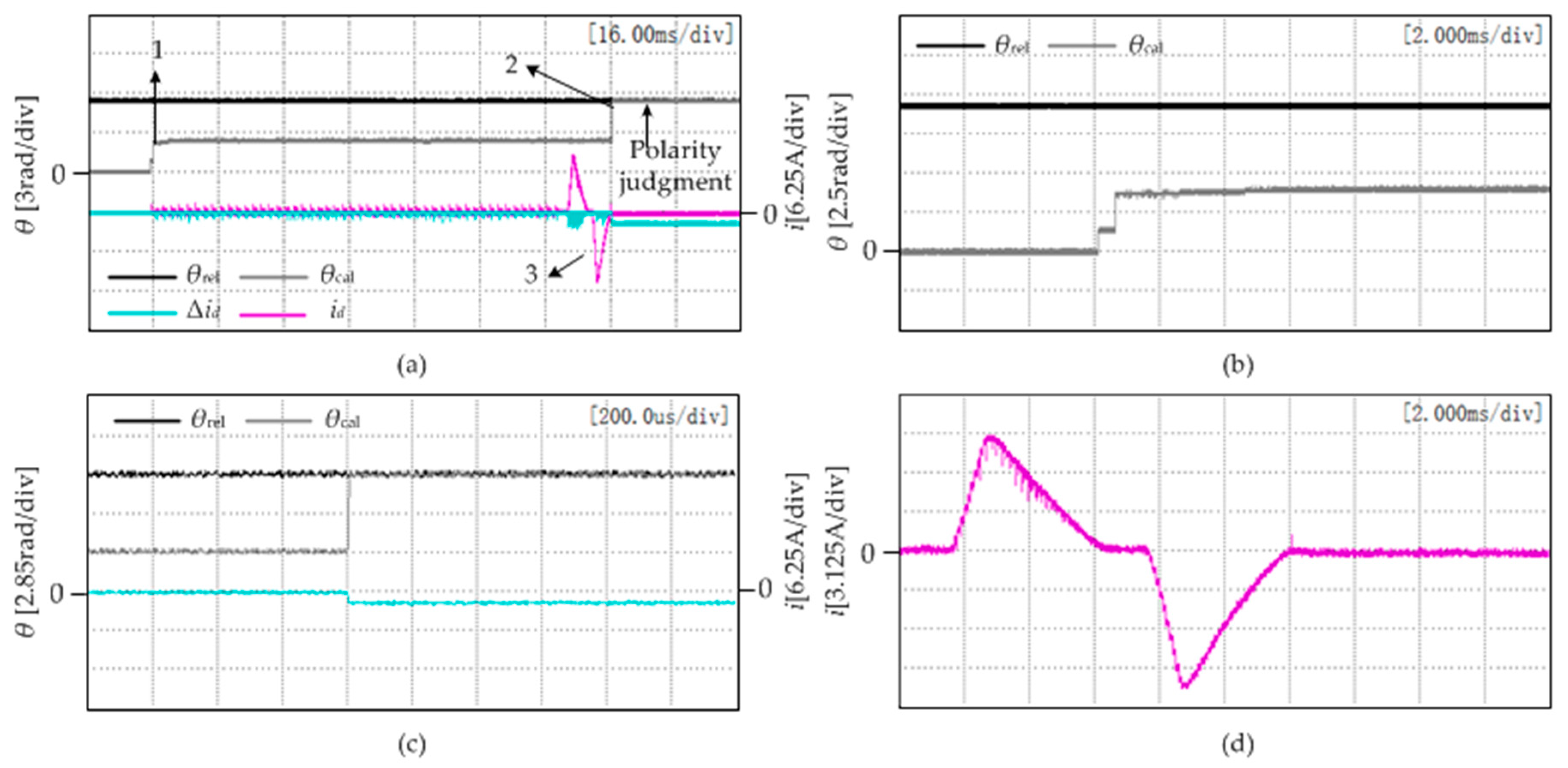
Figure 12a shows the actual and estimated positions of the rotor when the actual rotor angle is 88.7°. In the figure,
θrel is the true rotor position obtained by the resolver,
θcal is the angle obtained by the improved algorithm,
id is the current response when the positive direction injection and the reverse direction injection voltage are constant when the polarity is judged, and Δ
id is the difference in the current response.
In
Figure 12b, the calculation of the position angle takes about 8 ms. In
Figure 12c, When the polarity is judged, the positive value of Δ
id indicates that the current response during the d-axis forward voltage injection is larger than that in the negative injection, indicating |
id,
θ|>|
id,
θ + π|; therefore, it can be judged that the rotor position is at the N-pole,
θ =
θcal.
Figure 12d shows the current waveform of
id when injecting the high-frequency signal.
As shown in
Figure 13a, the actual position of the rotor was 307.33°. The rotor position is calculated after the polarity is determined. As shown in
Figure 13b, the calculation of the position angle takes about 8 ms.
As can be seen from
Figure 13a, the actual position of the rotor was 129.485° and the rotor position calculated before the polarity judgment is different from the actual position angle by π. In
Figure 13a, when the polarity is judged, Δ
id is negative, indicating that the current response when the d-axis forward voltage is injected is smaller than that of the negative injection, which is |
id,
θ|<|
id,
θ+π|; therefore, it can be judged that the rotor position is at the S-pole,
θ =
θcal + π.
Figure 13d shows the current waveform of
id when injecting a high-frequency signal.
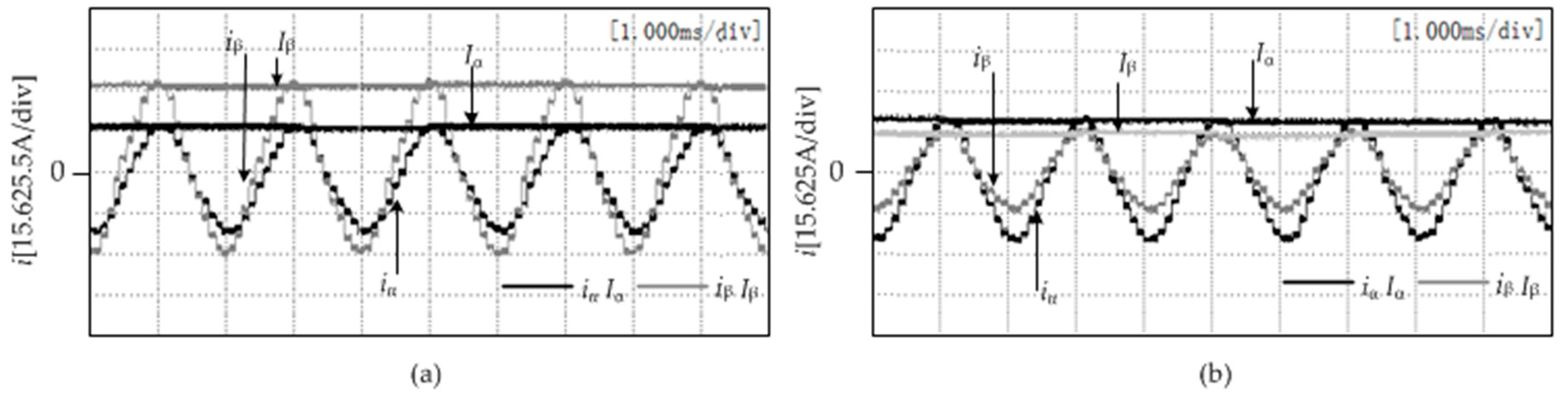
Figure 14a shows the high-frequency current response waveform when
θ = 88.7°.
Figure 14a shows the
iα,
iβ instantaneous values and the amplitudes
Iα,
Iβ containing the direct current component. When the rotor position is less than 90°,
iα is asymmetrical due to the mechanical asymmetry of the motor. In
Figure 14, the current amplitude obtained by the improved method is very accurate. The direct current component is calculated to be 25.25A, and after the direct current component is subtracted,
Iαθ = −9.63A,
Iβθ = 9.135A and the interval in which the current is located, that is, the interval
Iα- θ>
Iβθ>
Iαθ, and
θ = 90.765° can be obtained according to Equation (19). The error is mainly caused by the inaccuracy of current sampling. During the operation of the motor, the inductance will reverse, which leads to the difference between the current value and the theoretical value. This includes the fact that the DC component fluctuations ripple at a relatively accurate value in each experiment, which leads to errors in the values of
Iαθ and
Iβθ because the motor operates at zero speed and no load, so this the error will be very small. Comparing the result estimated by the formula with the actual result, it can be concluded that the error of position estimation is 2.07°.
Figure 14b shows the high-frequency current response waveform when
θ = 307.33°. After subtracting the direct current component,
Iαθ = −9.625A,
Iβθ = −6.49A, it can be judged that the current is in the interval, where
Iα- θ >
Iβθ >
Iαθ, and
θ = 129.485° can be obtained according to Equation (19). Since
θ can only calculate the value within π, as shown in
Figure 13d, the polarity can be judged by polarity judgment. The position angle should be added to π, and the estimated position angle is 309.485°. Compared with the actual position, the position estimation error is 2.15°.
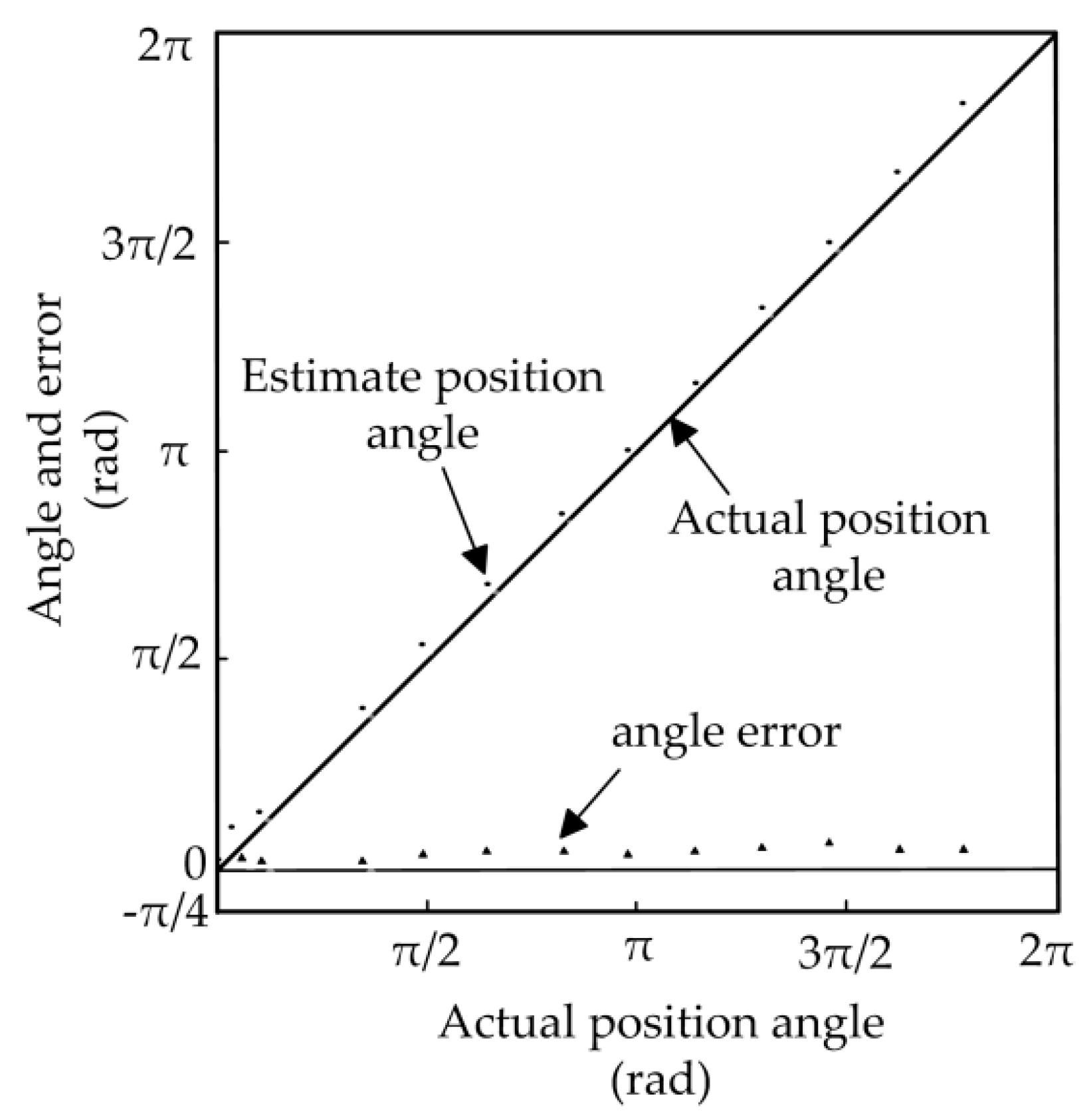
Figure 15 shows the comparison between the estimated value and the actual value of the rotor position. By changing the actual initial position of the motor, the actual initial position of the motor is increased from 0 rad to 2π rad at about every 0.55 rad interval. Compared with the calculated initial position of the motor,
Figure 15 is obtained. It can be seen from the figure that the maximum error is within 5°, the average error is approximately 2.7° and the detection error of the rotor position is relatively small. It has little effect on the start-up of the PMSM.
Although the accuracy of the initial position angle calculated by the traditional filter method is not different from that obtained by the proposed method, when the motor rotates, the method using the filter has a significant angle delay. This paper does not use the filter, so there is no angle delay. The experimental results are shown in
Figure 16.
From the above experimental results, it can be seen that the difference between the estimation of the rotor position detection value and the actual value is also small. The causes of the error are mainly the current sampling error, asymmetry of the motor structure, external disturbance of the system structure and current response error caused by different saturation degrees of the rotor in different positions. The current response has been averaged over several cycles to reduce the angular error of the rotor. In subsequent research, the number of periods of calculation can be increased to reduce angle error.
6. Conclusions
A rotor position detection method for a permanent magnet synchronous motor (PMSM) based on high-frequency voltage signal injection has been proposed in this paper. The rotating high-frequency voltage signal is injected into the stator winding. According to the relation between the amplitude of high-frequency current response and rotor position angle, the rotor position information is obtained using inverse tangent and linear formulae, then the polarity of the rotor is distinguished from the variation of the inductance.
This method is simple and easy to implement, does not depend on parameters and does not need to use a low-pass filter. It has good application value and can be used in engineering practices. This paper is mainly applied to the IPMSM. The main mathematical model is also for the IPMSM and has not been extended to the surface permanent magnet synchronous motor (SPMSM), which is a limitation of this paper. Later, the model will be analyzed and verified for the surface mounted motor. In addition, the high-frequency sinusoidal signal injection method adopted in this paper, which is limited in frequency, will affect the dynamic response performance of the system, and increase the interference between the fundamental and high-frequency signals.


