A Procedure to Estimate Air Conditioning Consumption of Urban Buses Related to Climate and Main Operational Characteristics

Abstract

Public Transport (PT) planning requires a detailed evaluation of the fleet energy consumption, usually depending on the specific characteristics of the bus service network. These include topography, climate and operational features. In this work, we focus on the additional air conditioning (AC) energy consumption, proposing a method to evaluate the extra energy consumption based not only on climate variables, but also on the PT planned service. Results are presented for a large part of the provincial capitals and regions of Italy, and clearly show that overconsumption for air conditioning are significantly affected by the daily mileage distribution, with large variance even when climatic conditions are similar. The mileage data are extracted from GTFS databases, widely available for PT applications. The developed tool allows us to apply this methodology to any urban and extra-urban area. Reference AC consumption related to climate conditions are derived from a measurement campaign hold in Cagliari (Sardinia, Italy) during September 2018, within the National Research Program on the Electric System. A discussion on how to optimize the use of climatic data is also presented, resulting in the choice to use Heat Index as unique independent variable for air conditioning energy consumption calculation. A methodology to compute the Heat Index from climatic variables for large domains as, for instance, the Italian regions, was also developed.

1. Introduction

Reference values for energy consumption and exhaust emissions for traction of Public Transport (PT) buses have been widely available for decades [1,2,3,4], in order to fulfill energy consumption and noxious emissions of National and Regional inventories of transportation activities. More recently, measures and analyses on Battery Electric Buses energy consumption have been carried on, as for instance by [5]. Datasets often include a large amount of details on vehicle technical characteristics, as engine technology, emission standard classes, or about environmental features, as morphology and traffic conditions. Unfortunately, most of these data sets do not consider the impact of on-board heating and cooling that, in some cases, as for battery electric vehicles (BEVs) technology, could be crucial to determine the effective vehicle range. More generally, heating, ventilation and air conditioning (HVAC) may have a not negligible impact on energy consumption and exhaust gas emissions, varying up to an order of magnitude as temperature and humidity changes.

The objectives of transport sustainability requires attention to the absorbing energy of all elements, whether the source power is electrical or not. As a matter of fact, consumption of electric energy can also have a major impact on climate and energy independence when power is produced mainly from fossil fuels and not for a sufficient quota from RES.

Research on this topic has been carried out by several authors [6,7,8,9,10,11,12]. In fact, a large part of the available studies is devoted to the detailed description of a specific vehicle or heating/conditioning system, while less work has been published about a general (even less accurate) description of the energetic impact of the HVAC systems related to the context where the vehicle is operating.

For this objective, several features should be considered. In particular, the hourly mileage distribution can have a major impact on HVAC consumptions: different peak hours in the bus service during the day can lead to large differences in HVAC consumptions, even for territories characterized by similar climates. For example, the average specific energy consumption for Air Conditioning in a small city, typically characterized by a double peak of the transit bus service in the morning and in the midafternoon, can be much lower with respect to the consumption of a large city, characterized by a high service rate during all working hours and in particular in daytime working hours when temperatures are the highest.

In this work, we propose a method to evaluate the air conditioning consumption for a transit bus fleet operating over a certain territory, starting from field measurements effected in other areas. We applied such a method to several Italian cities (all cities with more than 100,000 inhabitants) and regions and carried out descriptive charts of air conditioning consumption based on local climate and operational characteristics. We focused our analysis on electric vehicles since, differently from Internal Combustion Engine (ICE) vehicles, air-conditioning consumptions can be considered independent from traction consumption.

Section 2 describes the methods adopted to evaluate the impact of air conditioning systems on the energy consumption of buses according to local characteristics. The results are presented in Section 3, and the final conclusions (Section 4) close this work.

2. Bus Air Conditioning Usage Related to Local Climate

Usually, in Europe, consumption and exhaust gas emissions due to road vehicles operations are computed by adopting the COPERT tool [4,13,14]. Therefore, our analysis gets underway by taking into consideration the COPERT approach also to evaluate air conditioning consumption. Unfortunately, even the last version of COPERT considers the contribution of air conditioning apparatus for only a few vehicle categories, mainly cars and Light Duty Vehicles, and do not include buses. In order to fulfill this deficiency, willing to maintain continuity with COPERT methodology [15], we approach the problem using both a linear model [6] and monthly mean values for air temperature and humidity detected at two meters above the ground.

The Weilenmann et al. [6] model evaluates CO2 emissions and assumes no emission for temperatures lower than 5 °C. For higher temperatures, the consumption is computed as:

• A constant factor taking into consideration the consumption of a conditioning system working at a minimum rate for low temperatures (for which conditioning in principle should not be necessary)
• A linear contribution dependent on external 2 m temperature for environment temperatures higher than a threshold T_r larger than 5 °C.

Three curves are computed for different values of humidity (20%, 30% and 50%, respectively [15]) and the final result is given by a linear interpolation or extrapolation considering the actual value for humidity. The model computes CO2 emissions that are successively converted into energy consumption using a multiplication factor dependent on the type of fuel, the number of vehicles using air conditioning and the number of km run with the air conditioner switched on.

The parameters of the model are set by an analysis of real air conditioning systems performed during the 2000s. This approach requires the use of several observations in order to set accurate parameters for different values of humidity and temperature. At present, in COPERT, no data for buses is available. Moreover, in general, air conditioning consumption does not depend on the number of km travelled, but on the functioning power and time the system being turned on. The linearity of such a model allows us to use values for temperature and humidity averaged over long time periods, so that, in COPERT, monthly mean values are considered.

In our study, we analyze the air conditioning consumptions for electric buses, since they can be considered uncorrelated with the powertrain operation, and therefore, can provide an accurate estimation of the real energy required for heating and cooling. In fact, heat emitted from the thermal engines affects the bus cabin temperature, and can even be used to warm the cabin in winter.

In 2018 ENEA, within the Electric System Research Program, we performed a measurement campaign on a group of 12 m trolleybuses operating in Cagliari [16], equipped with on-board batteries in order to also run some mileage in the absence of the overhead contact line. The air conditioning device has a nominal power of around 12 kW, although the average input power during functioning is around 7.5 kW. The mean input power and climate data are available for 73 round trips (start to restart from the same terminal) performed during September 2018. These data have been used to achieve a model of cooling power as a function of air temperature and humidity.

Since the number of trips does not allow us to find sufficiently precise coefficients for a parametric function with two independent variables, i.e., temperature and humidity, we chose to use only one variable representing the perceived temperature computed as a combination of both temperature and humidity, i.e., the widely adopted Heat Index.

Heat Index is an empirically defined variable aimed at representing the physiological discomfort due to the combined action of temperature and humidity. This was proposed by Steadman [17] who considered temperatures higher than 28 °C and a limited range of humidity values. We follow the work of Anderson et al. [18], which generalize the definition of Heat Index and allows us to obtain values for any range of temperatures and humidity, in particular for low temperatures.

In Figure 1, the Heat Index in function of 2 m temperature and relative humidity is shown for the ENEA field campaign of September 2018 in Cagliari. We note that Heat Index is primarily linked to temperature, while only relatively small deviations can be associated to humidity. The use of Heat Index allows us to take into account the behavior of consumption in function of two variables, while at the same time limiting the degrees of freedom of the interpolations by the use of constrictions related to 30 years of experience of physiological discomfort.

In general, even if the available set of data is dominated by relatively low temperatures, not optimal for the use in the Heat Index context, we observed that the fit of the AC power in the function of Heat Index is always characterized by an increase in the explained variance (R2) with respect to the sole use of the Temperature. An example is reported in Figure 2, where the average power of the Air Conditioning system from stop to stop (including stop time) is shown as a function of both 2 m Temperature and Heat Index, for the ENEA measurements in Cagliari.

By observing Figure 2, we noticed that, for both temperature and heat index, the average round-trip power is quite low due to two reasons: (a) hourly temperatures (and heat index as well) not being very high, with respect to the peaks observed during summer season in many Italian regions; (b) low average Load Factor for the analyzed trips in Cagliari, out from both the touristic peak of summer holydays and the school opening period. This is a limitation of the available observations that needs to be improved in future work. Mean input power is 0 for Temperature values close to 20 °C (20 for heat index), meaning that the AC device has been switched on only for temperatures higher than 20 °C. This is consistent with the findings of other works [7].

Similar results are obtained considering daily averaged values, as shown in Figure 3: the interpolation parameters are similar to those in Figure 2, with a larger R2, even if the data pairs are too few to obtain stable results.

We therefore choose to force the interpolation line, by imposing that the AC power is zero for a Heat Index equal to 20. Results are shown in Figure 4 considering either all trips separately and daily averaged data. Plots are shown using all available data (left panels) or cutting out all data couples with a heat index lower than 20 (right panels).

Even if the experimental data are quite scattered, linear interpolation seems to fit enough for the objective of this analysis; nevertheless, a deeper investigation on possible different fittings and approximations will be carried out in future developments.

In all considered cases, the values of the coefficients of the fitting line are quite similar. We therefore define a model for the power consumption by the air conditioning system as follows:

$$P\left(HI\right)=\{\begin{array}{cc}\hfill 0,& \hspace{1em}HI<20\hfill \\ \hfill a\cdot HI+b,& \hspace{1em}HI\ge 20\hfill \end{array}$$

(1)

where HI is the heat index and a and b are the linear interpolation parameters, defined as a = 0.416, b = −8.314, respectively, corresponding to the values of the bottom right graph (panel d) in Figure 4. This model is valid in the event that the air conditioning system is capable of providing sufficient power for all possible heat index configurations, in particular never reaching the maximum power deliverable. Out of this condition, a constant curve needs to be included that is equal to the maximum power available, for a heat index higher than the threshold HI₀ = (Pmax − b)/a.

2.1. Air Conditioning Annual Consumption

Neglecting the losses of the electricity distribution and vehicle battery recharge/discharge, we can compute the AC energy consumption by multiplying the input power P by the time duration.

At the daily scale, as a first approximation, we could estimate air conditioning operation time as the ratio between the miles travelled L and the commercial speed v, including stop time, if computing the mean P along the same period.

More precisely, in order to consider the effective distribution of P(HI) along the day, we can compute the average number (n₂₀) of hours characterized by a heat index larger than 20 (HI₂₀). The resulting formula for average daily energy consumption of a single bus in month j is:

$$E_j^{day}=\frac{1}{\mu }·{\displaystyle \sum }_{i}P{\left(H{I}_{20}\right)}_{i,j}$$

(2)

where μ < 1 (approximately 0.85) represents electric pathway efficiency (line + battery), P(HI₂₀) is the mean AC input power at hour i and month j, and the summation is made over the hours when HI is larger than 20. For the typical operation time from 6.00 to 24.00, n₂₀ will be at least 18 or lower.

To compute n₂₀, we must individuate hourly heat indexes higher or at least equal to 20 within the operating time. This can be performed by adding two more variables to the daily mean Temperature: maximum and minimum average Temperature. We are therefore capable of approximately estimating the temperature variation during the standard day, choosing to use the approximate method CIBSE [19], widely used in literature and comprehensively described, for instance, by Chow e Levermore [20]. Similarly to the COPERT findings, the model is piecewise linear, so that we can apply it using long time averaged variables. We therefore chose to use monthly averaged values for temperatures. Following this approach, considering hourly intervals, the temperature at the hour i = 1…24 of the standard day of the considered month is computed as T_i = f_1,i T_min + f_2,i T_max with f_1,i + f_2,i = 1, defined in the function of i and of predefined parameters related to the hours when the maximum and minimum temperature peaks are observed. Figure 5 shows the hourly HI for the standard day of each month for Rome for example.

Estimation of air-conditioning consumption according to Equation (2) is useful in the absence of detailed daily data about the fleet service, but implies very strong assumptions, such as the uniform bus usage during the operation time and the invariance of the operating time among the buses.

In order to avoid these approximations, we can use information about the average use of the fleet during the day. In particular, if the total fleet mileage (veh-km) travelled along the representative day of each month j are available, the daily energy consumption for air conditioning of a single bus can be written as:

$$E_j^{day}={\displaystyle \sum }_i{P}_{i,j}·r_{i,j}/\mu$$

(3)

where

$$r_{i,j}=\frac{vehk{m}_{i,j}}{max\left(vehk{m}_{i,j}\right)}$$

(4)

r can vary between 0 and 1 and represents the percent usage of the effective operating fleet at hour i of the standard day of the month j. Unitary time factor under summation is implied.

We are therefore capable of estimating the AC energy consumption of a vehicle during the day as the correlation between the distribution of the hourly required energy for AC and the distribution of the vehicle-km, with a multiplying factor obtained by imposing that the full use of the fleet corresponds to the maximum value of the vehicle-km in the considered year

We note that a further improvement of this method could be the use of the hourly distribution of mean speed. In such a way we can remove the hypothesis that links the usage of the fleet to mileage values. In this case we can write: $e_{i,j}=\frac{P_{i,j}}{v_{i,j}}$, where $e_{i,j}$ represents the km consumption for month j and hour i, and $v_{i,j}$ represents the correspondent average speed in km/h.

The total energy consumption of the fleet during a day is therefore: $E_j^{day,fleet}={\displaystyle \sum }_i{e}_{i,j}·{vehkm}_{i,j}$ so that the energy for each vehicle is obtained dividing E by the total number of buses in the fleet. Hourly mean speeds can be easily estimated from GTFS data only if both length and times from stop to stop is available while data on bus fleet composition are generally available from PT companies.

Data on the distribution of vehicle-km can be derived for instance by the analysis of the GTFS data provided by local transport companies, as described below.

2.2. Representation of Mileages by Means of the GTFS Data

The daily distribution of mileages required for the computation of the HVAC consumptions (see Section 2.1) can be obtained by analyzing the GTFS data (General Transit Feed Specification, see for instance Reference [21]) available from the local public transport companies. The use of these data is rapidly growing so that, even if at present, this format is not universally adopted, it is possible to foresee broad use in the next years. In this study, we chose to use a limited number of GTFS data representative for different types of territory contexts, because the availability of the data is still limited. In addition, we preferred to use data related to the year 2019, in order to avoid temporary effects associated with the impact of the COVID-19 pandemic. Obviously, specific GTFS data of each territory can be considered for a more precise evaluation of the AC energy impact.

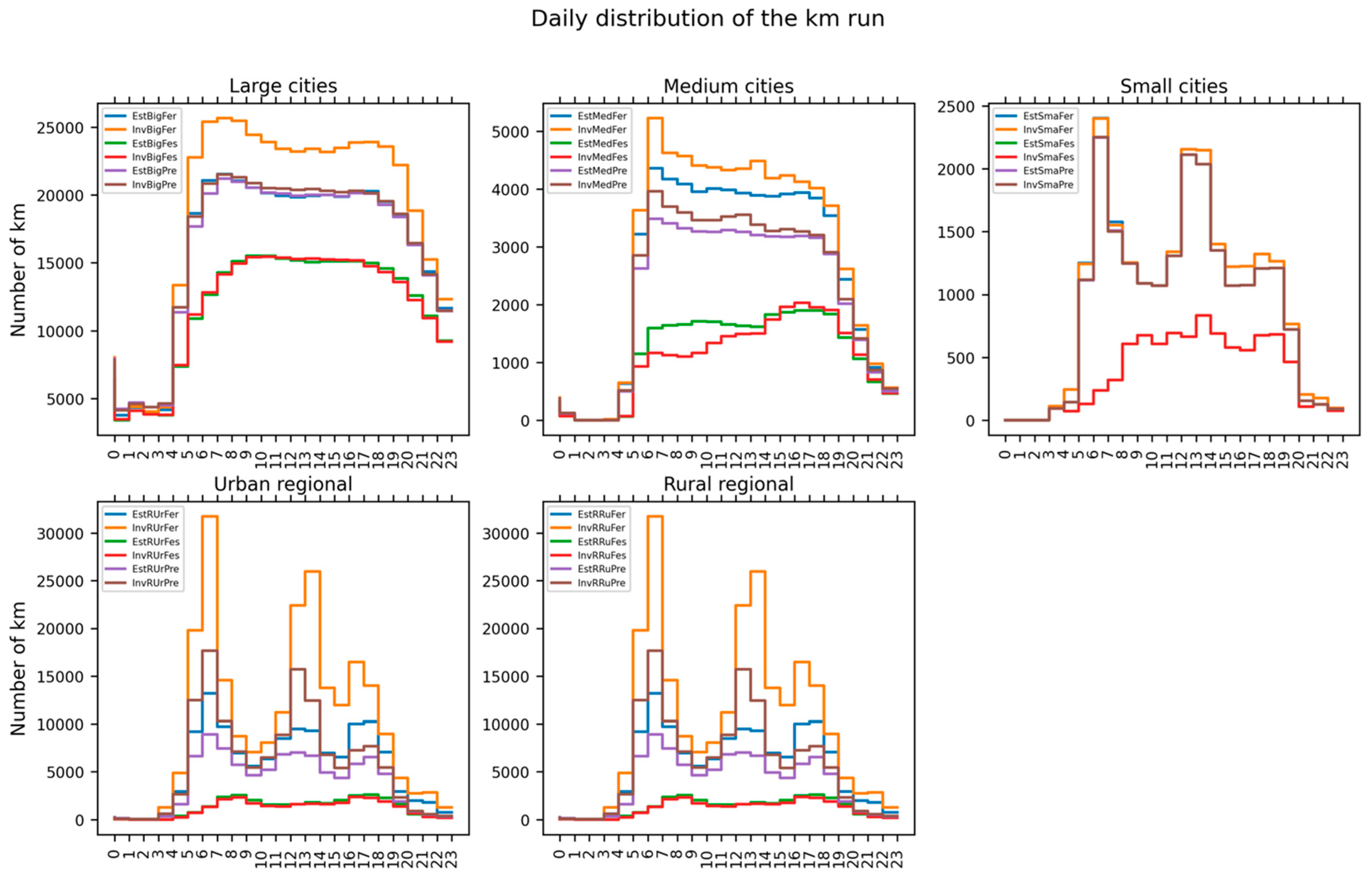
Figure 6 represents the summer and winter distributions of mileage for working days, preholiday and holidays, respectively. Graphs for urban PT in large, medium and small cities are shown, as well as for regional urban and non-urban bus services. The classification is based on population: cities are defined as ‘large’ if they have more than 500,000 inhabitants, ‘small’ with less than 100,000 inhabitants, while medium cities are characterized by a number of inhabitants within 100,000 and 500,000. The Rome GTFS file has been used for large cities, Florence and Livorno files for medium and small cities, respectively. For regional distribution, we used the Piedmont GTFS file for both urban and rural services, since at the time of writing no reliable separate GTFS data for urban and extra-urban trips were available to the authors. Data representative for a standard working, holiday and preholiday day for summer and winter are shown, respectively, with a summary of the chosen days reported in

Table 1. Reference territories and dates used to compute the fleet mileage distributions shown in Figure 6. Dates are expressed as YYYY/MM/DD.

Type of Territory	Reference Territory	Summer Working	Summer Holyday	Summer Preholiday	Winter Working	Winter Holiday	Winter Preholiday
Large	Rome	2019/07/31	2019/08/04	2019/08/03	2019/10/18	2019/10/20	2019/10/19
Medium	Florence	2019/09/06	2019/09/08	2019/09/07	2019/11/20	2019/11/24	2019/11/23
Small	Livorno	2019/09/16	2019/09/22	2019/09/21	2019/11/20	2019/11/24	2019/11/23
Regional	Piedmont	2019/07/31	2019/08/04	2019/08/03	2019/11/27	2019/12/01	2019/11/30

.

2.3. Representation of Temperature at Regional Scale

Representing environmental variables over regional scales can be difficult, due to the non-homogeneity present along large geographical areas. Differences may arise from morphology, as the presence of sea, plains and mountains in the same region, or from a different land use, as urban and rural environments. Our approach requires the use of a single value to represent Temperature or Humidity at the regional scale, so that we require choosing an acceptable approximation to perform our task.

When considering cities, our choice is to refer to a weather ground observing station representative for the city area, preferably characterized by a long data series allowing for the calculation of the monthly average minimum, mean and maximum temperature and humidity. In Italy, weather ground observation data are handled and owned by each Region, yet at least part of them is centrally available for the entire territory through the ISPRA web servers, by means of the SCIA service [22], at the web address: http://www.scia.isprambiente.it/wwwrootscia/Home_new.html#, accessed on 20 January 2021.

For the representation of the variables over a wider area, for instance the regional domains, different approaches are possible (see page 185 and following of Riva and Murano [23], or the introduction of Begert and Frei [24] and references therein):

• Keep a representative ground station of the entire region
• Classify the region in terms of climatic zones (by means of heating degree days)
• Compute area average of the available stations belonging to the region
• Compute area average of fields available over a regular grid from a regional analysis or re-analysis.

The climatic zones were originally defined in Italy in order to classify the territory by the energy needs for winter building heating. More recently, extensions of the method have also been proposed to take into account energy needs for summer air conditioning [23]. However, summer and winter methodologies differ; moreover, the climatic zones are defined by means of degree-day, so that it is not straightforward to associate a climatic zone to monthly averaged values of temperature and humidity.

The use of regional analysis or re-analysis allows us to obtain data over a regular grid derived from numerical weather models and observations, so that variables can also be reconstructed in locations where no real observation is available. For the Italian territory, high resolution analyses or re-analyses are not easily available; more importantly, even if they represent the best theoretical estimate of the variables in the space of the numerical model, we note that it is not convenient to include it in the computation values defined at any grid point of the domain, with the risk of including non-representative values, as for instance temperatures over a mountain crest. Handling these problems is beyond our aims; in addition, the resolution of the grid is not necessarily optimal to represent the scale of the environmental variables required for transport needs, with the risk of working with non-representative quantities.

Our choice is therefore to describe the environmental variables on the regional scale by means of a single station or an average of representative stations in the region. In particular, we point out that, for regional transport systems, most of the trips are located within or close to the larger centers, so that the use of a weighted average of temperature and humidity representative of the province capitals can be a sufficient approximation. Supposing that the intensity of the bus service is proportional to population, we can adopt this parameter for weighting climate variables over the region. The use of a denser meteorological network, without detailed information on the real distribution of public transport on the area, is associated to the risk of non-representative results, with too large weights to meteorological stations located in places that are not representative of the public transport distribution.

This approach can be easily followed, since meteorological data are available at the already mentioned ISPRA site [22] and also data on population distribution are publicly available at the ISTAT website (I.Stat: http://dati.istat.it/Index.aspx, accessed on 10 January 2021).

3. Air-Conditioning Consumption for Italian Territories

Applying the method described in Section 2.1, and using the total mileage distribution obtained by the GTFS data described in Section 2.2, we are capable computing the annual distribution of consumptions for cooling of an electric bus in a specific area. We note that this method can be easily applied in most countries, since data from ground weather stations and for cities’ population is in general available everywhere, and the GTFS format is based on an international agreement and is almost universally adopted to represent public transport data. However, it is advisable to carry out specific functions that correlate average AC functioning power and HI, reflecting effective use of AC at the local level.

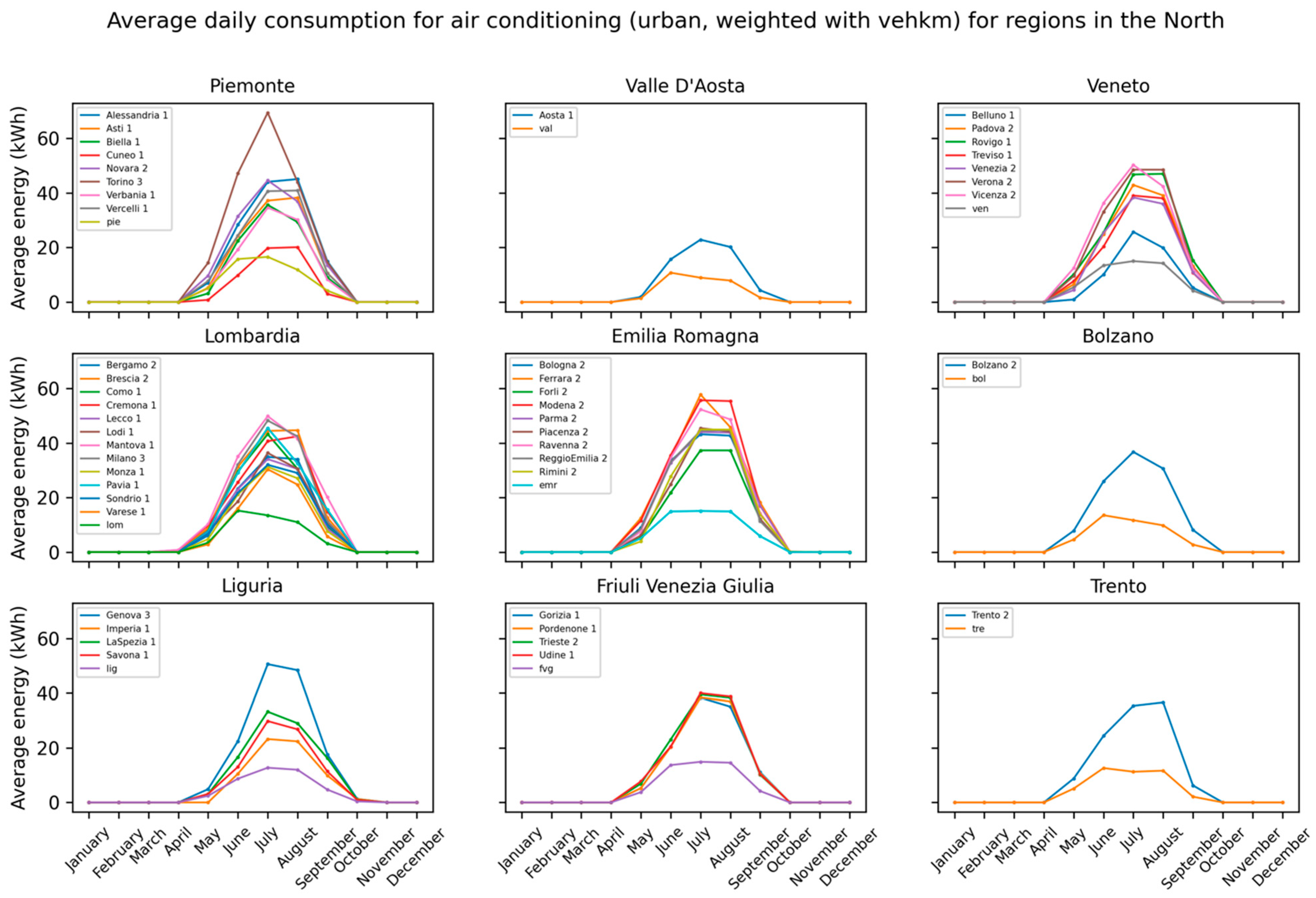
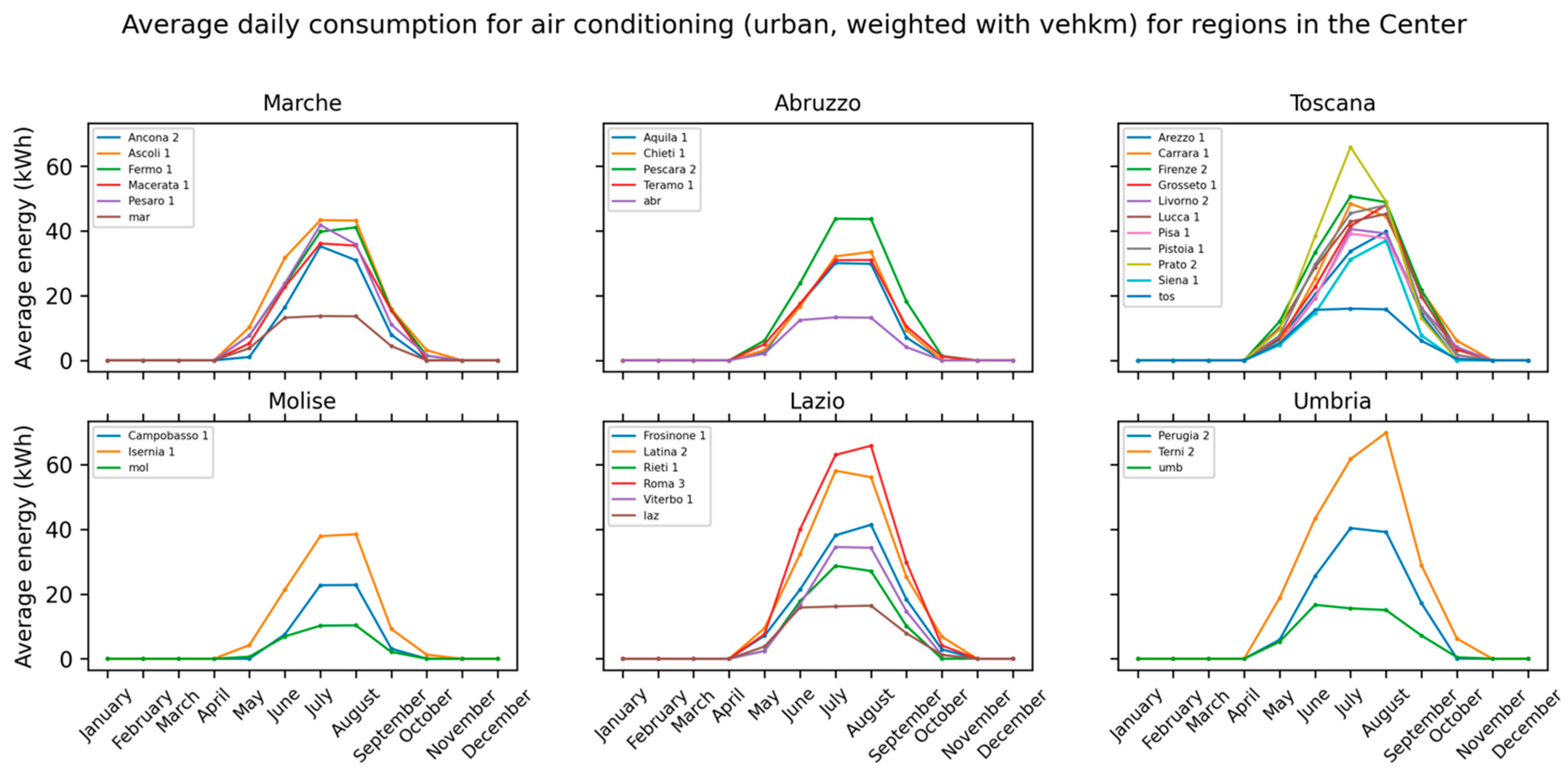
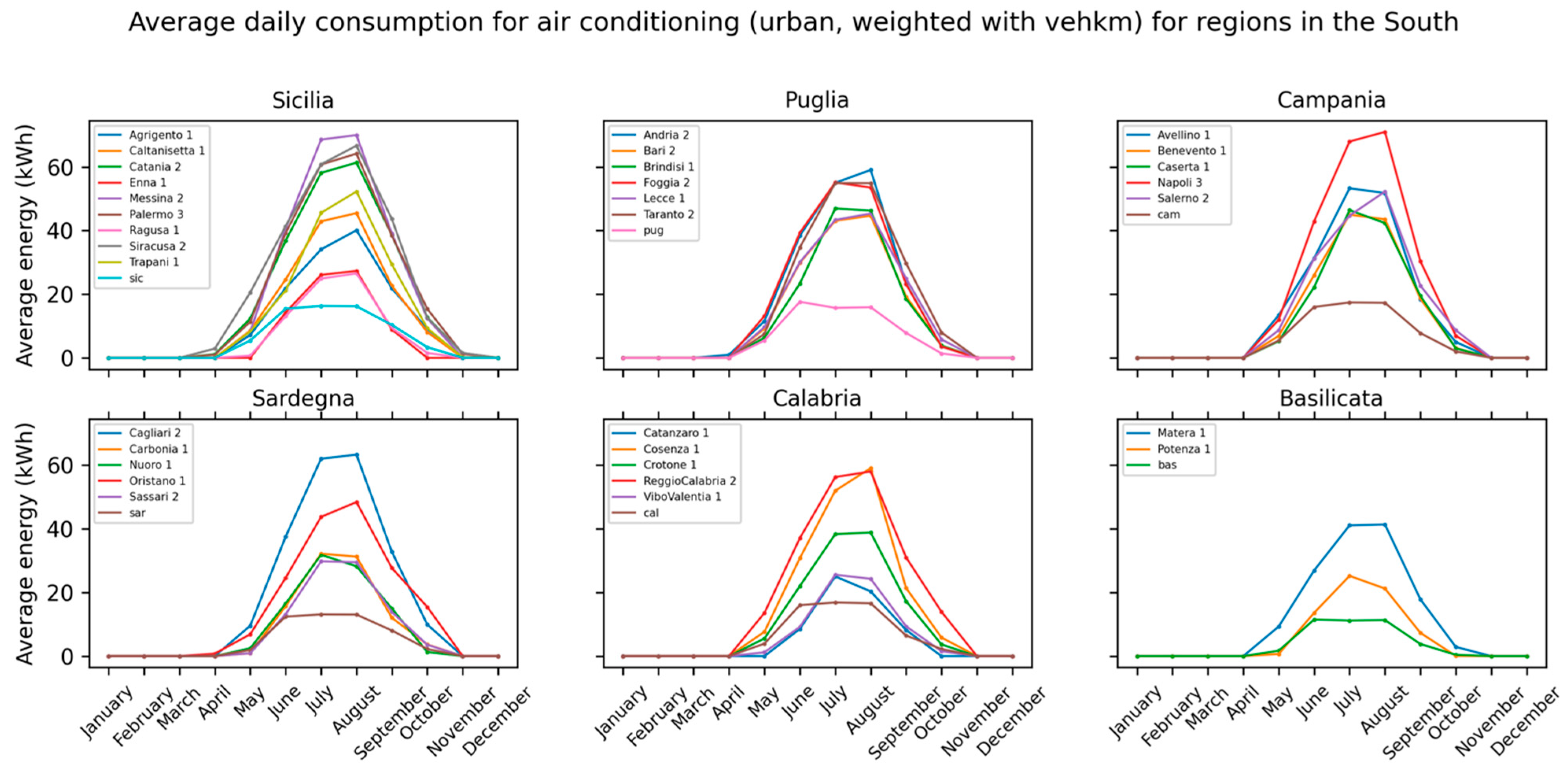
In Figure 7, Figure 8 and Figure 9, the estimates of the air-conditioning energy consumption are reported for each month for all the province capital cities of the regions in the Northern, Central and Southern Italy, respectively, applying the linear functions of input power vs. Heat Index derived from experimental data, as described in Section 2.

The classification of the cities as large (3), medium (2), or small (1) is reported in the figures’ legend, next to the city name. We grouped city and regional results in three macro regions (North, Center and South), usually adopted to describe statistics in Italy, also because the climatological differences among the three areas. In fact, large differences are also observed within the macro-regions, mainly due to the presence of the Alps and the Apennines mountain chains and to the different impacts of the Mediterranean Sea. However, our choice is to privilege the latitude of the territories as the primary climatic factor for classification, in general with higher summer temperatures when moving toward the South. In spite of this, summer temperatures with very high humidity values are often experienced in the Po valley, located in the Northern part of Italy, or in smaller valleys of the Center, as for instance the Florence plain in Tuscany. On the contrary, southern regions, even if affected by higher temperatures on average, are often characterized by lower humidity values.

The contribution of cooling is represented by the summer peaks. The results are presented for all province capitals, either because of the relevance of these cities themselves or because we require these data in order to compute regional weighed average temperature, heat index and consumption values, as stated in Section 2.3. Regional consumptions are in general lower than those of the cities due to the different distributions of the trips within the day, in particular with less trips during the late morning hours, and therefore less energy needs for air conditioning.

The impact of the mileage distribution is apparent. As a matter of fact, some regions are characterized by roughly constant climatic variables through the entire territory, as in the case of Liguria, shown in the bottom left panel of Figure 7: the four province capitals are all close to the sea and have relatively small differences in latitude and morphology. Three of the four cities are classified as small cities, while Genova is classified as large. The resulting consumptions are consistent with the city classification, with similar contributions for Imperia, La Spezia, and Savona, while much higher consumptions are estimated for Genova. Similar results characterize the Lazio region, while the impact of the climatic differences is apparent in other regions, as for instance Basilicata or Umbria, where all the cities are associated with the same vehicle-km distribution, but show different consumptions due to variations in average temperature and humidity. These two effects are mixed in other regions, in particular in the largest regions characterized by complex morphology and with province capitals belonging to all city classes, for example Sicilia or Veneto.

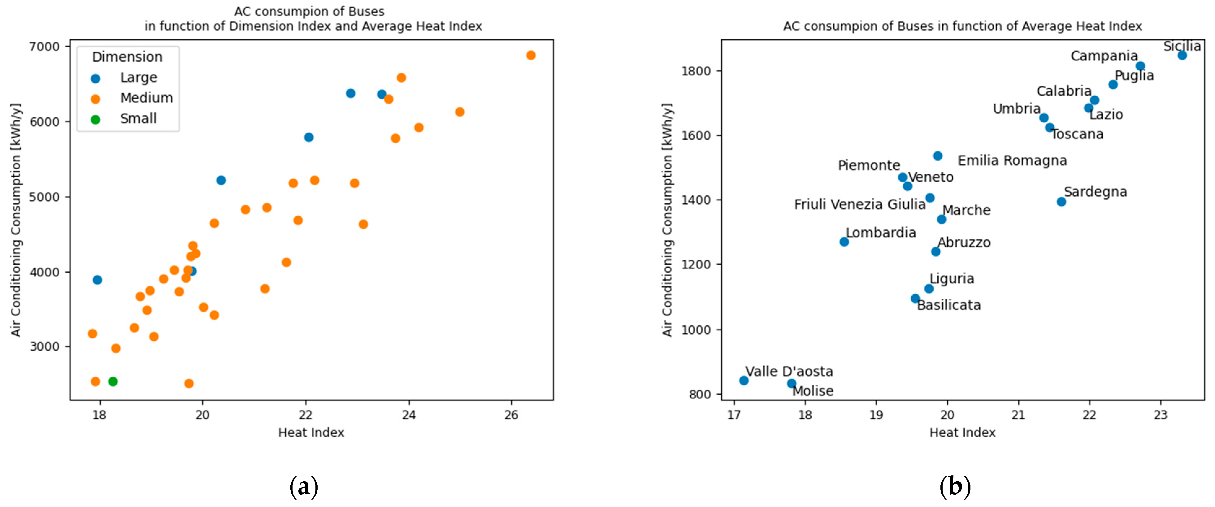
The consumptions for air conditioning are well correlated with Temperature and Heat Index, respectively, as shown in Figure 10 for all types of cities. In particular, it is clear that, by considering the three different city dimensions separately, and consequently the three reference mileage distributions, the consumptions are well correlated to the climatic variables, showing the potential of using more detailed mileage distribution in the future in order to better characterize the HVAC consumption of the single territory. It is worth noting that the values of the annual AC energy consumption for each Dimension Index in Figure 10 do not lay over a line due to the fact that our method considers climatic variables for each month, as well as the temperature distribution within the standard day, so that a not negligible impact is represented by the temperature excursion and by the behavior of temperature and humidity throughout the year. Similar results are obtained for the regions.

According to the previous estimates, at the yearly scale, cooling energy consumption can account for ten percent with respect to traction energy consumption; in fact, if we assume, for a 12 m electric bus, a mean yearly mileage of 40,000 km and an average specific consumption of 1.2 kWh/km, the energy required for traction and other minor auxiliaries amounts to around 50 MWh, versus a maximum of 7 MWh for cooling, in the hottest cities. These results must be considered as lower-bound references, due to the particular on-site measurement conditions they derive from, namely both low buses load factors and low outside temperatures, with respect to peak summer conditions in Italy. In any case, they show that technical efforts to increase traction energy efficiency could be invalidated from the HVAC consumption, extending the results obtained for cooling needs also for heating.

Moreover, critical issues could arise in electric buses daily operation, in burdensome winter or summer climate conditions, when HVAC energy request could limit the maximum daily range. As a matter of fact, in these particular days of the year, energy needs for HVAC could even be comparable with the consumption for traction and other minor auxiliaries. In addition, mainly in winter time, together with the highest heating needs, battery capacity can be reduced. Spot biberonages during operation, the so called “opportunity re-charge”, as well as the In Motion Charge (IMC), could help in removing electric buses range limits, even reducing the needed battery capacity.

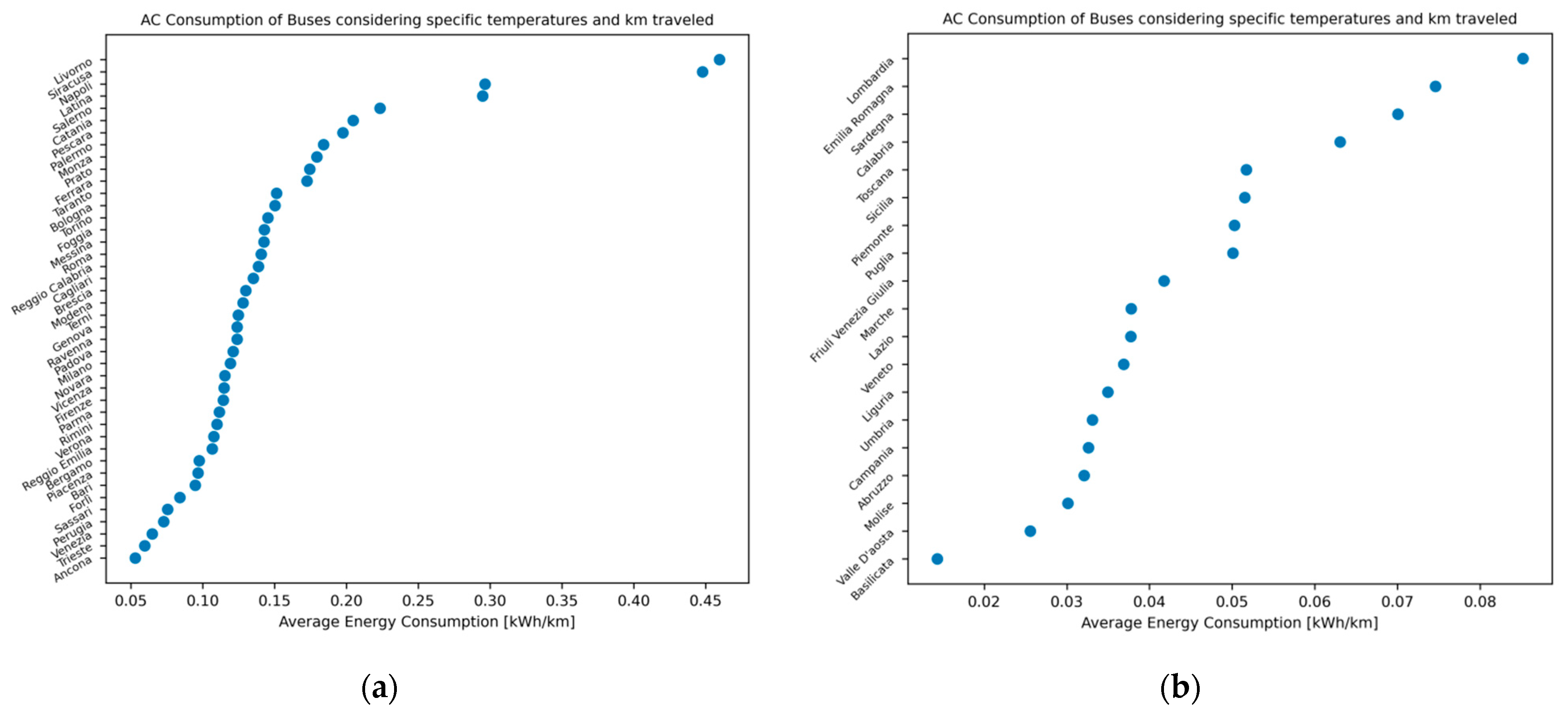
In order to compare traction and air conditioning energy needs, it could be useful to estimate the average HVAC energy consumption per km, dividing the annual consumption by the annual mileage of a single bus. This latest value can be obtained elaborating GTFS data on planned service and acquiring information on fleet composition from PT Companies.

As an example of such an application, we recur the average 2017 annual mileages estimated by INVITALIA for the Italian Strategic Sustainable Mobility Plan monitoring, for all the Italian regions and cities with a population larger than 100,000 inhabitants (see

Table 2. 2017 Average annual mileage traveled by a single bus in each territory considered in this work.

City	Km/Year	City	Km/Year	Region	Km/Year
Ancona	39,405.31	Palermo	31,504.83	Abruzzo	35,340.46
Bari	39,949.43	Parma	33,223.76	Basilicata	66,989.52
Bergamo	28,029.54	Perugia	46,545.72	Calabria	24,010.16
Bologna	24,513.08	Pescara	18,025.42	Campania	50,545.49
Brescia	30,384.84	Piacenza	36,910.73	Emilia Romagna	15,815.67
Cagliari	42,334.78	Prato	26,901.99	Friuli Venezia Giulia	35,557.55
Catania	25,849.21	Ravenna	33,224.43	Lazio	38,731.98
Ferrara	24,318.01	Reggio Calabria	37,117.37	Liguria	28,505.74
Firenze	40,273.27	Reggio Emilia	35,186.07	Lombardia	14,287.33
Foggia	32,335.38	Rimini	31,663.95	Marche	33,407.43
Forlì	34,118.53	Roma	39,045.86	Molise	24,148.79
Genova	28,564.24	Salerno	19,099.82	Piemonte	27,898.8
Latina	15,260.93	Sassari	32,229.71	Puglia	31,902.87
Livorno	6874.796	Siracusa	13,428.32	Sardegna	19,081.45
Messina	42,930.78	Taranto	30,808.39	Sicilia	31,386.46
Milano	30,412.5	Terni	46,799.57	Toscana	30,462.82
Modena	36,661.14	Torino	33,143.95	Umbria	40,933.08
Monza	13,973.63	Trieste	58,350.22	Valle d’Aosta	33,891.63
Napoli	19,342.94	Venezia	43,577.7	Veneto	35,295.96
Novara	32,283.03	Verona	36,446.4
Padova	28,241.12	Vicenza	35,330.24

Source: INVITALIA analysis for National Strategic Plan of Sustainable Mobility monitoring.

). Applying these mileages to the energy consumption shown in the previous graphs, we obtain the results in Figure 11 for cities and regions, respectively. According to these estimates, even neglecting outlayer values, AC average consumption per km can rise up to 0.25 kwh/km, i.e., up to 20% of the traction consumption (for a reference value of 1.2 kWh/km). Moreover, further energy consumption is expected for heating needs, so that HVAC total consumption are of the same order of magnitude as traction consumption, even at the annual scale. Of course, more detailed analyses are required for single territories, as the results shown in Figure 11 clearly show important differences, pointing out the importance of a local analysis to differentiate the energy demands of specific territories.

As shown in Figure 10, yearly consumptions are in general well correlated with averaged heat index, even if an important role is also associated with the trip distribution during the daytime.

4. Conclusions

In this study we propose an analysis of the impact of the peculiar characteristics of a territory on the air-conditioning consumption of buses for public transportation. A new method is proposed that considers both the trip distribution over a day and the climate variables.

This analysis is relevant in allowing local administrators to correctly allocate re-sources to guarantee an optimal public transport service; for instance, to allow for the correct dimensioning of the batteries of electric vehicles, or more generally to choose those technologies or operation strategies that can significantly reduce energy consumption from auxiliaries.

As a matter of fact, electric consumption, as it is for AC devices in most cases, must be limited as much as possible in order to comply with the objectives of transport sustainability, mainly if power production does not provide a sufficient quota of RES.

Results show large differences among the Italian territories, in large part related to the climatic differences, but also with an important contribution due to the mileage distribution associated with the area. Different usages of the fleet can lead to different energy needs for the air-conditioning, even in similar climatic conditions. In our study, this is apparent when comparing cities with similar climatic characteristics, but different bus services, classified by size and type categories.

We propose to describe the mileage run by the bus fleets by means of the GTFS data. The importance of a correct description of the vehicle-km distribution of a territory is pointed out throughout this work, with the consequent that, if the GTFS data were available for each considered territory, their impact could be even larger than that observed in this work. The improvement in the use of GTFS is one of the goals of future work, as we are confident that, in the future, a wider diffusion of these data from the bus companies can bring us to a more detailed analysis of the distribution of the fleet usage during a standard day. Since the GTFS format is composed of compulsory parts and optional fields, future improvements in our analysis will also allow us to fully exploit the GTFS data in any available format.

Results presented in this work are only a part of the analysis required in order to completely assess the energy needs of public transportation in a specific territory. The energy required for heating and hilliness are the other two main contributions not considered in this work. An approach similar to the one described for AC can be adopted to study the heating impact on energy needs, while a COPERT like approach can be used to evaluate the impact of topography on consumptions through GTFS data. Future improvements of our work will be devoted to the inclusion of these two topics in order to build a comprehensive evaluation of the total energy needs of the local territories.

Moreover, we stressed the importance of improving the quality of the observed data for air conditioning consumptions presented in Section 2. In particular, we stress that the number of observations presented in this work is suboptimal, even if it allows for a stable characterization of the interpolations. The observation campaign has been performed during the first half of September, so that few data associated to temperatures higher than 28 °C are available, with the consequence that we need an extrapolation of the observed data to compute consumptions related to the most energy demanding climate conditions of several Italian locations during the summer period. Moreover, since the beginning of September in Cagliari is neither a high tourist season nor working peak period, the observed values of air-conditioning power are related to low values of the buses load factor. As a consequence, the energy consumption estimates may be undervalued due to the low stress of the air conditioning system during the observation campaign, and more work needs to be performed in order to strengthen the results.

In spite of the weaknesses described above, the method we proposed is capable of providing consumptions that are consistent with the available studies, with the additional value of simultaneously taking into account the climatological and population profiles of local territories, and the further strength of being easily exportable to any territory, since only widely available tools are involved in the analysis.