Article

Hierarchical Model Predictive Control for Autonomous Collision Avoidance of Distributed Electric Drive Vehicle with Lateral Stability Analysis in Extreme Scenarios

National Engineering Laboratory for Electric Vehicles, Department of Mechanical Engineering, Beijing Institute of Technology, Beijing 100081, China
*
Author to whom correspondence should be addressed.
World Electr. Veh. J. 2021, 12(4), 192; https://0-doi-org.brum.beds.ac.uk/10.3390/wevj12040192
Submission received: 13 September 2021 / Revised: 7 October 2021 / Accepted: 12 October 2021 / Published: 15 October 2021

Abstract

:
This paper proposes an active collision avoidance controller based on a hierarchical model predictive control framework for distributed electric drive vehicles (4IDEV) considering extreme conditions. In this framework, a two-layer strategy is developed. The upper layer is the path replanning controller based on nonlinear MPC (nMPC), from which a collision-free path including the optimal lateral displacement and yaw angle can be obtained in real-time while encountering the obstacles. The lower layer is the path tracking controller based on hybrid MPC (hMPC), and the coordinated control inputs (yaw moment and the front wheel steering angle) are solved by a Mixed-Integer Quadratic Programming (MIQP) with the piecewise affine (PWA) tire model considering tire saturation region. Moreover, to improve the lateral stability when tracking, the stable zone of lateral stability in the high-risk condition is analyzed based on the phase portrait method, by which the constraints of vehicle states and inputs are derived. The verification is carried out on the MATLAB and CarSim co-simulation platform, and the simulation results show that the proposed active collision avoidance controller can track the reference path accurately and prevent vehicle instability in extreme scenarios.

1. Introduction

In recent years, many countries have attached great importance to environmental problems, especially focusing on electric vehicles (EVs). The four in-wheel-motor drive electric vehicle (4IDEV), one of the most advanced structures of EVs due to its advantages of high transmission efficiency and unique actuated system layout, has developed rapidly. Facing the complex traffic environment nowadays, the problem of how to ensure 4IDEV’s driving stability and safety in an extreme maneuver becomes a hot topic among scholars’ research [1,2,3,4]. The extreme maneuvers can be described as driving on a low coefficient road surface at high speed. Four independent motors, providing the driving torque and braking torque, are installed on each wheel of 4IDEV. Its novel driving layout shows advantages to handle lateral stability when suffering the worst-case scenario.
It is crucial to create a safe path that is also easy to track when meeting an unexpected condition. In contrast to global planning, local planning is used to cope with emergency scenarios. There are several methods to solve a local planning problem like the Artificial Potential Field (APF) -based method [5,6,7], sample-based method [8], optimization-based method [9,10], and interpolation curve-based method [11,12]. The sample-based method is a fast-computing way to obtain feasible trajectories in real-time, combined with the multi-objective optimal algorithm, the best path can be selected from the trajectory cluster [13]. In addition, the optimal path can also be generated by general quadratic programming (QP) [14]. In [15], a risk assessment MPC-based local path planning algorithm was proposed based on the predicted trajectories of surrounding vehicles. In [16], social behaviors were taken into consideration when solving the MPC problem. However, effectively solving an optimization problem is extremely dependent on high-computing performance, consequently the interpolation curve-based methods such as Polynomial Curves [17,18], Bezier Curves [19], etc., are widely used to reduce the computation.
Path tracking performance is extremely essential to handle vehicle stability, especially in a high-risk driving scenario. Various methods such as H∞ control [20,21] and slide mode control (SMC) [22,23] are usually applied in the path tracking control of 4IDEV. The model predictive control (MPC), due to its advantage to forecast the future status of the controlled system, is commonly used in the path tracking of intelligent vehicles. Based on different control inputs, the MPC-based method can be divided into three aspects as follows: active front steering (AFS), direct yaw-moment control (DYC), and coordinated control. In [24,25], the AFS based on combining the Linear Time-Varying MPC (LTV-MPC) with the PID feedback control was proposed. Ref. [26] presented a DYC method based on MPC using the bicycle model with lagged tire force for a better description of the vehicle behavior. Comparing with DYC, ref. [27] used the lateral force of the front tire as the control input of MPC, and the enveloped stable zone is defined based on motion analysis of the stable point in the phase portrait with different steering inputs. In order to improve the control capabilities, a switched MPC strategy of coordinated steering angle and yaw moment on low-friction is used in [28]. What’s more, ref. [29] conducted a multi-objective stability analysis (handling improvement, lateral stability, rollover prevention, and slip control) using the MPC approach with coordinated control.
A hierarchical control scheme combing planning controller and path tracking controller is typically used in collision avoidance problems [30]. Ref. [31] used a two-layer controller structure, and the upper layer adopted a path planning controller with a 3-D virtual dangerous potential field function, the lower layer adopted multi-constrain MPC to track the path. In [17], the upper planner integrating the predicted velocity based on the optimization method with the Polynomial Curves cluster, and an improved composite nonlinear feedback (CNF) control was presented for tracking. Ref. [32] constructed a robust combined lateral and longitudinal integrated controller in the scene of high-speed lane changing, in which the lower path tracking controller adopts sliding mode control. In [33], The upper controller for motion planning was created by using a friction-limited particle model, and the lower controller used a nonlinear 3DOF model Modified Hamiltonian Algorithm (MHA) for optimal brake and steer control allocation.
In general, the simplified vehicle model without considering the nonlinearity region of the tire is utilized in the control system to reduce the computing load, however, the control model accuracy hugely influences results in the high-risk and limit scenario [34]. From the aspect of keeping the vehicle off saturation, like in [35], it was shown how to modify dynamically the reference signals in order to compensate for the lack of control action of actuators entering a possible saturation condition. Some hybrid approaches to the management of the actuator saturations were also proposed in [36]. Another methodology of stability analysis in vehicle control based on the phase portrait of vehicle dynamics has been studied in many research studies [22,23,27,37], however, the regular pattern of stable points motion is still needed to be found. In this paper, a hierarchical predictive framework in an extreme autonomous collision avoidance maneuver is conducted. The optimal collision avoidance trajectories are generated by nonlinear MPC under limit road condition constraints, and the PWA tire model is used in a hybrid MPC strategy, in which the additional multi-constrain is obtained by analyzing the motion regularity of the stable point.
The rest of the paper is organized as follows: Section 2 deduces the kinematics and dynamic model of the 4IDEV including a PWA tire model, and the phase portrait analysis is conducted; Section 3 introduces the hierarchical control scheme in collision avoidance scenario comprised of nMPC and hMPC; Section 4 presents the simulation results considering the extreme condition and the conclusions are drawn in Section 5.

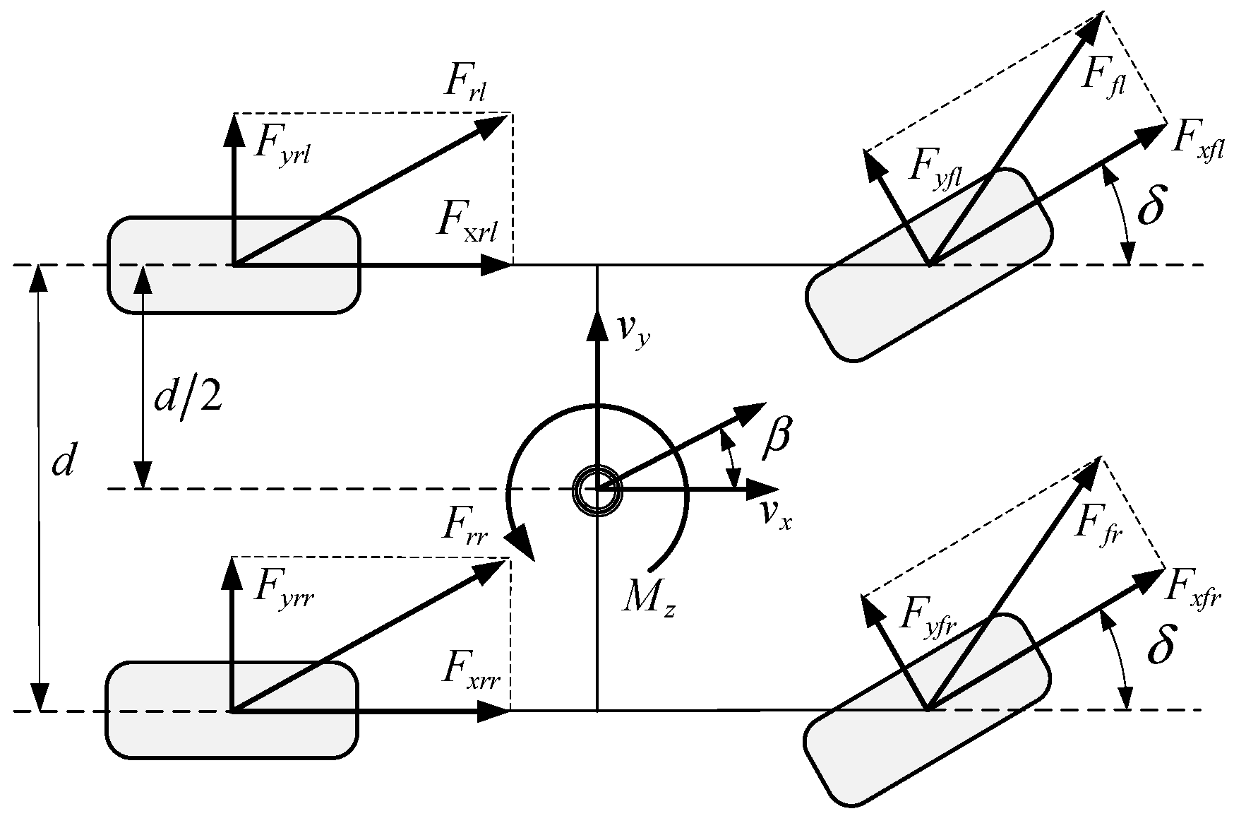
2. Distributed Drive Vehicle Model

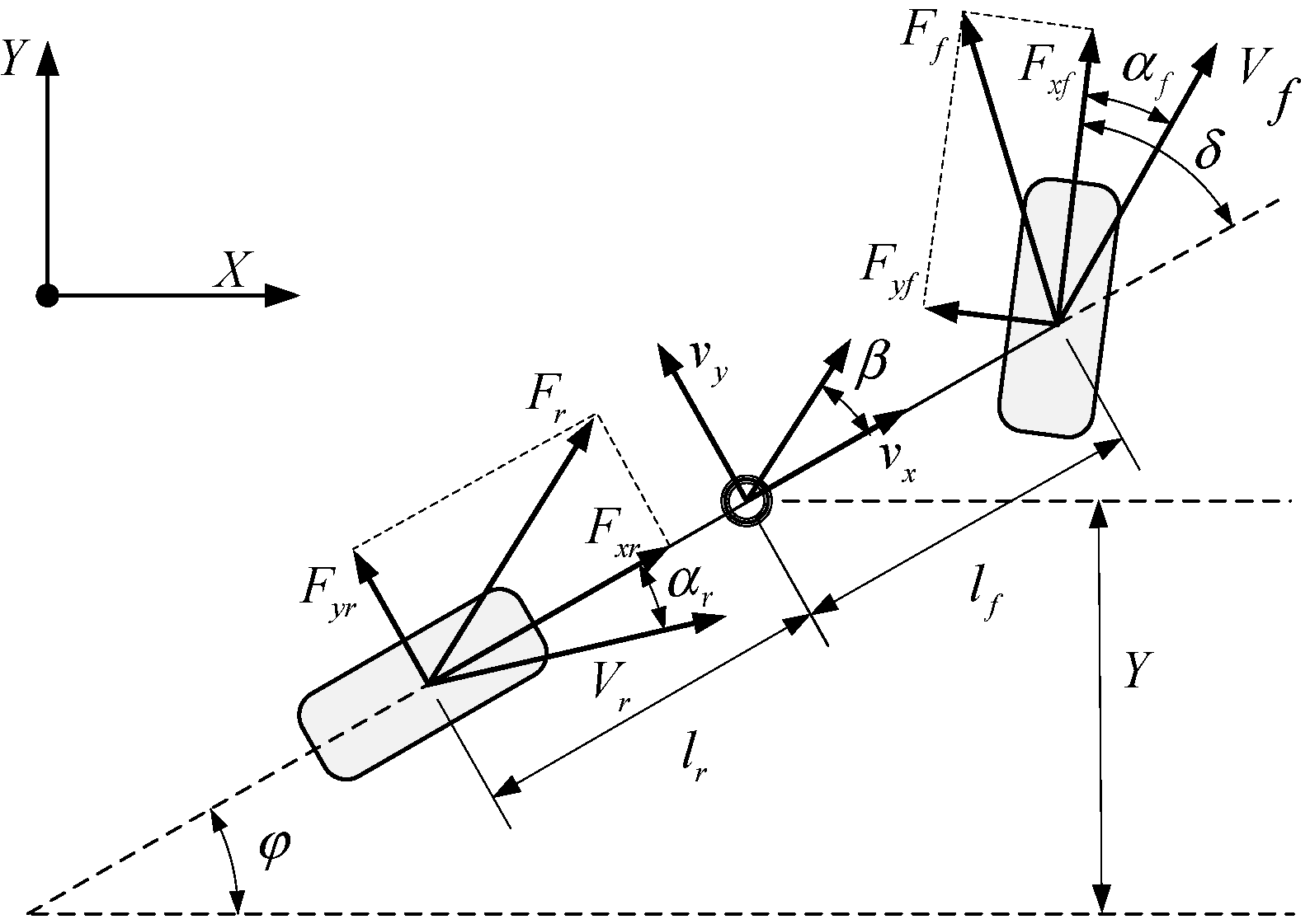
2.1. Vehicle Kinematics Model

To improve the efficiency of the solution, a simplified vehicle kinematics model is used in the path planning controller, as follows in (1), where X and Y are the longitudinal and lateral coordinates in the global coordinate system, v x and v y are the longitudinal and lateral velocity in the vehicle coordinate system, and φ is the vehicle yaw angle.
{ v ˙ y = a y φ ˙ = a y / v x Y ˙ = v x sin φ + v y cos φ X ˙ = v x cos φ v y sin φ

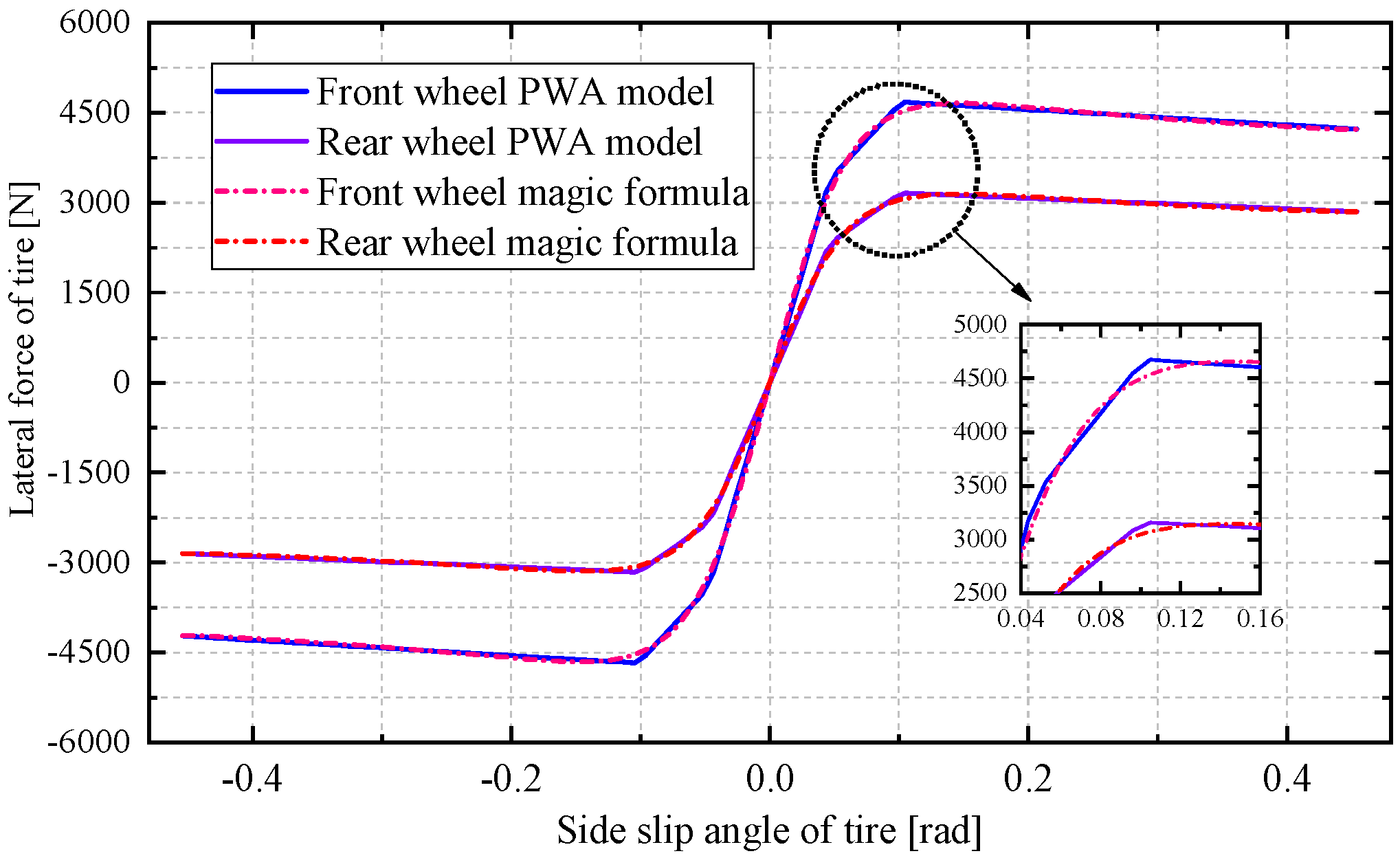
2.2. Piecewise Affine Vehicle Lateral Dynamics Model

The lateral force of the tire has a nonlinear relationship with the tire sideslip angle that may cause a huge amount of computation when solving the optimization problem, for which it’s difficult to calculate directly in the original nonlinear MPC algorithm. To approach the real driving scenario, in this paper, a piecewise linear function is applied to describe the characteristic of tires, then a hybrid model can be constructed by a PWA of magic tire model shown below in (2), where F y i is the lateral force of the right and left tire, B , C , D , E are the paraments affected by the tire characteristics, k 2 i , k 1 i , c i are the line slope, b 2 i , b 1 i are the line intercept, α i max , α 2 i , α 1 i are the segregating points, and the subscript i { f , r } represents the front and rear wheels.
F y i = D sin { C arctan [ B α i E ( B α i arctan ( B α i ) ) ] } { k 2 i α i b 2 i   if   α i ( α i max , α 2 i ) k 1 i α i b 1 i   if   α i [ α 2 i , α 1 i ) c i α i   if   α i [ α 1 i , α 1 i ] k 1 i α i + b 1 i   if   α i ( α 1 i , α 2 i ] k 2 i α i + b 2 i   if   α i ( α 2 i , α i max ]
The fitting curve based on a piecewise linear function is obtained by the universal global optimization (UGO) method and divided into five regions shown in Figure 1. The results illustrate that the fitting curve is extremely approximate to the tire magic function.
Figure 2 shows the structure of the 2DOF bicycle model. This model simplified the complicated vehicle dynamic model by only considering the lateral and longitudinal motion and setting the longitudinal velocity to a constant value. The lateral force and moment formula deduced by the bicycle model is shown below in (3), m is the vehicle mass, M z is the yaw moment, I z is inertia along the z-axis, l f and l r are the distance from the center of gravity to the front and rear axis, and F y f and F y r are the lateral force of front and rear wheels.
m v x ( β ˙ + r ) = F y f + F y r I z r ˙ = l f F y f l r F y r + M z
By assuming the longitudinal velocity v x and lateral velocity v y of the four-wheel are the same as one of the center of mass, the front and rear sideslip angle α f and α r can be calculated as follows, where the δ is the front wheel steering angle.
tan ( α f + δ ) = v y + l f r v x , tan α r = v y l r r v x
The sideslip angle at the center of mass can be defined as: β = v y / v x , so the sideslip angle at wheels are represented:
α f = β δ + l f r v x , α r = β l r r v x
In the global frame, when the yaw is small, the vehicle lateral motion is defined as:
Y ˙ = v x sin φ + v y cos φ v x φ + v y = v x ( φ + β )
Based on Equation (6), we can obtain:
Y ˙ = v x L ( l r α f + l f α r + l r δ + L φ )
Equations (2)–(7) are simplified to the form of the differential equation, hence we can obtain the hybrid vehicle lateral dynamics model as follows in (8), where the k f m , b f m , k r m , b r m represent the m t h region of the PWA tire model.
{ β ˙ = ( k f m + k r m ) m v x β + [ ( l f k f m l r k r m ) m v x 1 ] r k f m m v x δ + ( b r m + b f m ) r ˙ = ( l f k f m l r k r m ) I z β + ( l f 2 k f m + l r 2 k r m ) I z v x r l f k f m I z δ + M z I z + ( l f b f m l r b r m ) I z φ ˙ = r Y ˙ = v x ( l f + l r ) ( φ β + 2 l r δ ( l f + l r ) )
In Equation (9), the yaw moment is calculated from the longitudinal forces of four independent wheels. By controlling the four in-wheel-motor, the yaw moment can be exerted on the vehicle by applying differential torque. F x f r , F x f l , F x r r , F x r l , respectively, represent the longitudinal forces as shown in Figure 3.
M z = d 2 ( F x f r + F x f l cos δ F x r r + F x r l cos δ ) d 2 ( F x f r + F x f l F x r r + F x r l ) = d R 2 ( T x f r + T x f l T x r r + T x r l )

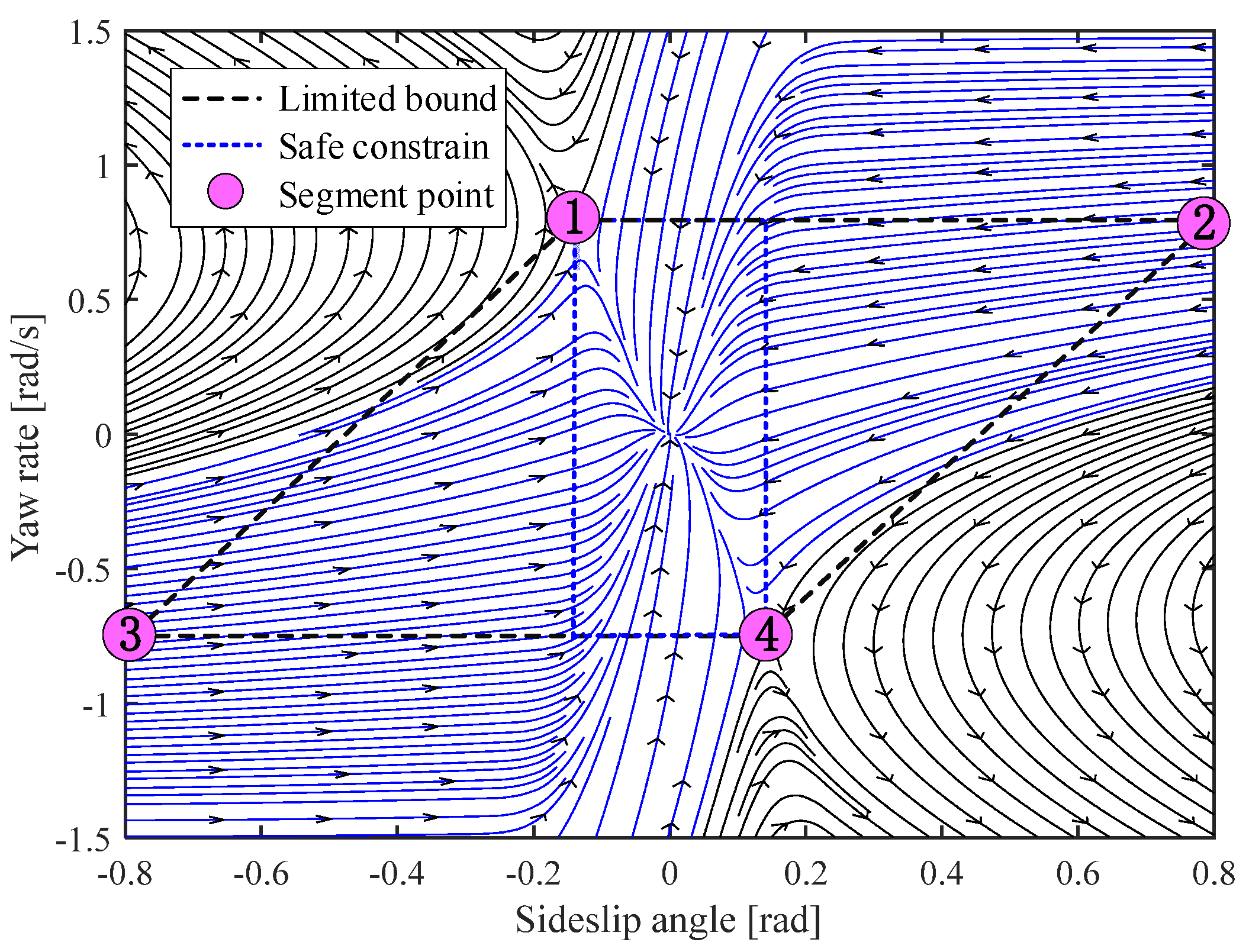
2.3. Stability Region Analysis Based on Phase Portrait

The front-wheel steering angle has a great influence on the change of β - r phase portrait. Figure 4 and Figure 5 show the phase portrait based on Equation (8) of the sideslip angle and yaw rate with different steering angles: 0 rad, 0.1 rad, 0.25 rad, 0.35 rad. The fixed points marked as blue or red can be directly found in Figure 4, respectively, the blue point represents the stable equilibrium point that the domain around which is convergent, and the red points are saddle points showing bifurcation behavior, which can be regarded as the boundary points between stable region ③ and unstable region ① and ② depicted in the streamline of a different color. For searching the motion law of the fixed points, we set the derivatives of the sideslip angle and yaw rate to zero and decouple the expression with β ˜ and r ˜ , then we can obtain (10):
β ˜ = ( M z k f m l f M z k r m l r + M z m v x 2 + b r m k f m l f 2 + b f m k r m l f l r + b r m k f m l f l r δ k f m k r m l r 2 b f m l f m v x 2 δ k f m k r m l f l r + δ k f m l f m v x 2 ) ( k f m k r m l f 2 + 2 k f m k r m l f l r + k f m k r m l r 2 k f m m l f v x 2 + k r m m l r v x 2 ) r ˜ = v x ( M z k f m + M z k r m b f m k r m l f + b r m k f m l f b f m k r m l r + b r m k f m l r + δ k f m k r m l f + δ k f m k r m l r ) ( k f m k r m l f 2 + 2 k f m k r m l f l r + k f m k r m l r 2 k f m m l f v x 2 + k r m m l r v x 2 )
We build a two-dimensional matric A ˜ for the next analysis based on Equation (11), where the κ represents the rest part that is not relative to β and r .
[ β ˙ r ˙ ] = A ˜ [ β r ] + κ s . t .   A ˜ = [ k f m + k r m m v x k f m l f k r m l r m v x 2 1 k f m l f k r m l r I z k f m l f 2 k r m l r 2 I z v x ]
Different kinds of fixed points can be judged by the eigenvalue λ { λ 1 , λ 2 } of the matrix A ˜ , the classification is expressed as follows:
  det ( A ˜ λ I ) = 0 { i f λ 1 λ 2 0 det ( A ˜ ) 0 { λ 1 > 0 , λ 2 > 0 unstable   point λ 1 < 0 , λ 2 < 0 stable   point i f λ 1 λ 2 < 0 det ( A ˜ ) < 0 saddle   point
When setting the steering angle δ from −0.35 to 0.35 rad, the trace of different fixed points at various steering angles can be described as the blue and red solid lines shown in Figure 4a,b, respectively, represent the trace of stable point and saddle point. The diamond blue points are terminal positions of stable point motion. In Figure 4a–d, the fixed point moves along the calculated trace with δ increasing. When the steering angle reaches up to 0.35rad, the stable point has disappeared at the terminal position, after that there is no stable region in the whole area. By analyzing the regular pattern of the phase portrait, the boundary and safe constraints can be presented as shown in Figure 5. The segment points are obtained by the saddle points position, all the coordinates are: (−0.1,0.77), (0.8,0.77), (−0.8,−0.74), (0.2,−0.74), by which a working area to ensure practical stability for the system is obtained.

3. Hierarchical Controller Design

The hierarchical control scheme proposed is shown in Figure 6, in which the upper controller calculates the desired lateral coordinate and yaw angle to avoid the collision, and the lower controller tracks the desired path, calculates the output with desired front-wheel steering angle and yaw moment.

3.1. Path Planning Controller Based on Nonlinear MPC

The path planning controller uses nMPC with the kinematic model mentioned in Section 2. Due to the equations being combined with the nonlinear functions, it is necessary to linearize the equations by solving the Jacobian matrix. The state-space can be written as follows in (13), the subscript n of which is represented the relative parameters in the nMPC controller.
x ˙ n = A n x n + B n u n y n = C n x n
where x n , y n , u n , A n , B n , C n are:
x n = [ v y v x φ Y X ] T y n = [ φ Y ] T u n = a y A n = [ 0 0 0 0 0 0 0 0 0 0 0 a y v x 2 0 0 0 cos φ sin φ v x cos φ v y sin φ 0 0 sin φ cos φ v x sin φ v y cos φ 0 0 ] B n = [ 1 0 1 v x 0 0 ] C n = [ 0 0 1 0 0 0 0 0 1 0 ]
In order to solve a finite time horizons problem, a k t h sampled discrete state-space form is obtained in (15). The superscript * represents discretization.
x n ( k + 1 ) = A n * x n ( k ) + B n * u ( k ) y n ( k + 1 ) = C n * x n ( k )
The optimization problem can be written as Equation (16), where the J k is the cost function at each time step k , combined with the tracking error prediction sequence Y n , k Y ref , k , inputs prediction sequence u n , k , and the obstacle cost J o b j , where Y ref , k is the initial desired reference. The optimal target is to solve the a y to minimize the cost function. We also add the constraints to prevent a y exceeding the road adhesion limitation.
{ min J k = min k k + N 1 ( Y n , k Y ref , k Q 2 + u k R 2 + J o b j ) s . t . μ g u μ g
The obstacle cost function J o b j , k is shown below in (17), which increases when the distance between the vehicle and obstacle reduces. The J o b j is the sum of the prediction sequence J o b j , k , S v r , k is the obstacle avoidance coefficient, ( x k , y k ) represents the current position of the vehicle in global Coordination, ( x 0 , y 0 ) is the coordination of obstacle position, N is the predictive horizon.
J o b j = k = 1 N J o b j , k = k = 1 N [ S v r , k ( x k x 0 ) 2 + ( y k y 0 ) 2 ]
We use a polynomial (19) to generate a collision-avoidance curve including the value of the optimal yaw φ r e f and lateral coordinate ζ r e f which are both the function of X , where p y 1 p y 5 , p φ 1 p φ 5 are fitting coefficients calculated by the predictive sequence Y n , k as shown in (18).
Y n , k = [ y n k | k y n k + I | k y n k + N I | k ] N T N
{ ζ r e f ( X ) = p y 1 X 4 + p y 2 X 3 + p y 3 X 2 + p y 4 X + p y 5 φ r e f ( X ) = p φ 1 X 4 + p φ 2 X 3 + p φ 3 X 2 + p φ 4 X + p φ 5

3.2. Path Tracking Controller Based on Hybrid MPC

The PWA vehicle lateral model mentioned above is used to construct the hMPC controller. According to Equation (20), a state-space form when the α f and α r are in m t h the region can be expressed in (21), where the subscript h is represented as the relative parameters in hMPC controller.
x ˙ h = A h x h + B h u h + g h y h = C h x h
Among which x h , y h , u h , A h , B h , C h , g h are:
x h = [ β r φ Y ] T y h = Y u h = [ δ M z ] A h = [ ( k f m + k r m ) m v x ( l f k f m l r k r m ) m v x 1 0 0 ( l f k f m l r k r m ) I z ( l f 2 k f m + l r 2 k r m ) I z v x 0 0 0 1 0 0 v x L 0 v x L 0 ] B h = [ k r m m v x 0 l f k f I z 1 I z 0 0 2 l r v x L 2 0 ] g h = [ b r m + b f m l f b f m l r b r m I z 0 0 ] C h = [ 0 0 0 1 ]
Generally, the system constructed above can be considered as a hybrid system that could be solved by the hMPC algorithm. However, the finite time horizon control problem of hMPC is a Mixed-Integer Quadratic Programming (MIQP) problem, which needs to convert the logic relations into the Mixed-Integer linear inequalities [38]. τ ( k ) is the logic switch component defined in τ ( k ) { 0 , 1 } , which is judged by the piecewise affine rules given in Equation (2). Based on (2) and (5), the switched rule expressed in matric form is in (22), where η ( k ) = [ β ,   r ] T , H p , G p , W p are the matric calculated by (2) and (5). The subscript p represents the number of inequalities obtained by the PWA tire model, which can be obtained by p = m 2 .
[ τ p = 1 ] [ H p η ( k ) + G p W p ]
According to the (2), we define z ( k ) = F y , the PWA tire model can be expressed in the if-and-only-if condition shown in (23), where a 1 and f 1 can obtain by (22).
z ( k ) = { a 1 η ( k ) + f 1   if   τ 1 ( k ) = 1   a p η ( k ) + f p   if   τ p ( k ) = 1
Equation (24) above is equivalent to (23):
{ z ( k ) = j = 1 p [ a p η ( k ) + f p ] · τ j ( k )   s . t . j = 1 p τ j ( k ) = 1    
By adding the auxiliary real vectors z ( k ) and logic components τ ( k ) , we can model the PWA system in the MLD form shown in (20). The matric A h * , B h 1 * B h 5 * , E 1 E 5 are determined by the HYSDEL [39].
x h ( k + 1 ) = A h * x h ( k ) + B h 1 * u h ( k ) + B h 2 * τ ( k ) + B h 3 * z ( k )   y h ( k ) = C h * x h ( k ) E 1 τ ( k ) + E 2 z ( k ) E 3 x h ( k ) + E 4 u h ( k ) + E 5
The optimization problem expressed in Equation (26) is similar to the nMPC problem, where Y h , k ζ ref , k represents the prediction sequence tracking error between current lateral displacement and the replanning path value obtained by (19), Δ u h , k is the prediction sequence of inputs’ increment between ( k 1 ) t h and k t h sample. Under the constraints analyzed in Section 2, the optimal value of the MIQP problem shown in (26) can be calculated by the hMPC algorithm at each receding horizon.
{ min J k = min k k + N 1 ( Y h , k ζ ref , k Q 2 + Δ u h , k R 2 )   s . t . β min β ( k ) β max φ min φ ( k ) φ max δ min δ ( k ) δ max M z min M z ( k ) M z max

4. Simulation and Results Analysis

The performance of the hierarchical controller is discussed in this section. The control strategy proposed was tested in the Simulink & CarSim co-simulation platform and the simulation time is set to 25 s. Considering the nonlinear characteristic of tires mostly reflects the handling performance in extreme scenarios such as driving on a low-coefficient road with a rapid steering angle and high speed, the simulation will test on the snow road that the adhesion of the road is 0.2 with the longitudinal velocity set to 54 km/h. Two scenarios are carried out in the simulation: the double lane change (DLC) scenario and the single lane with collision avoidance scenario. The performance of the lower path tracking controller using hMPC is compared to which using conventional linear MPC from the perspective of tracking errors and computational time. The RMSE of tracking errors is given by Equation (27), where n u m represents the number of simulation data. The vehicle simulation parameters are presented in Table 1.
R M S E = 1 n u m i = 1 n u m ( Y i Y r e f , i ) 2

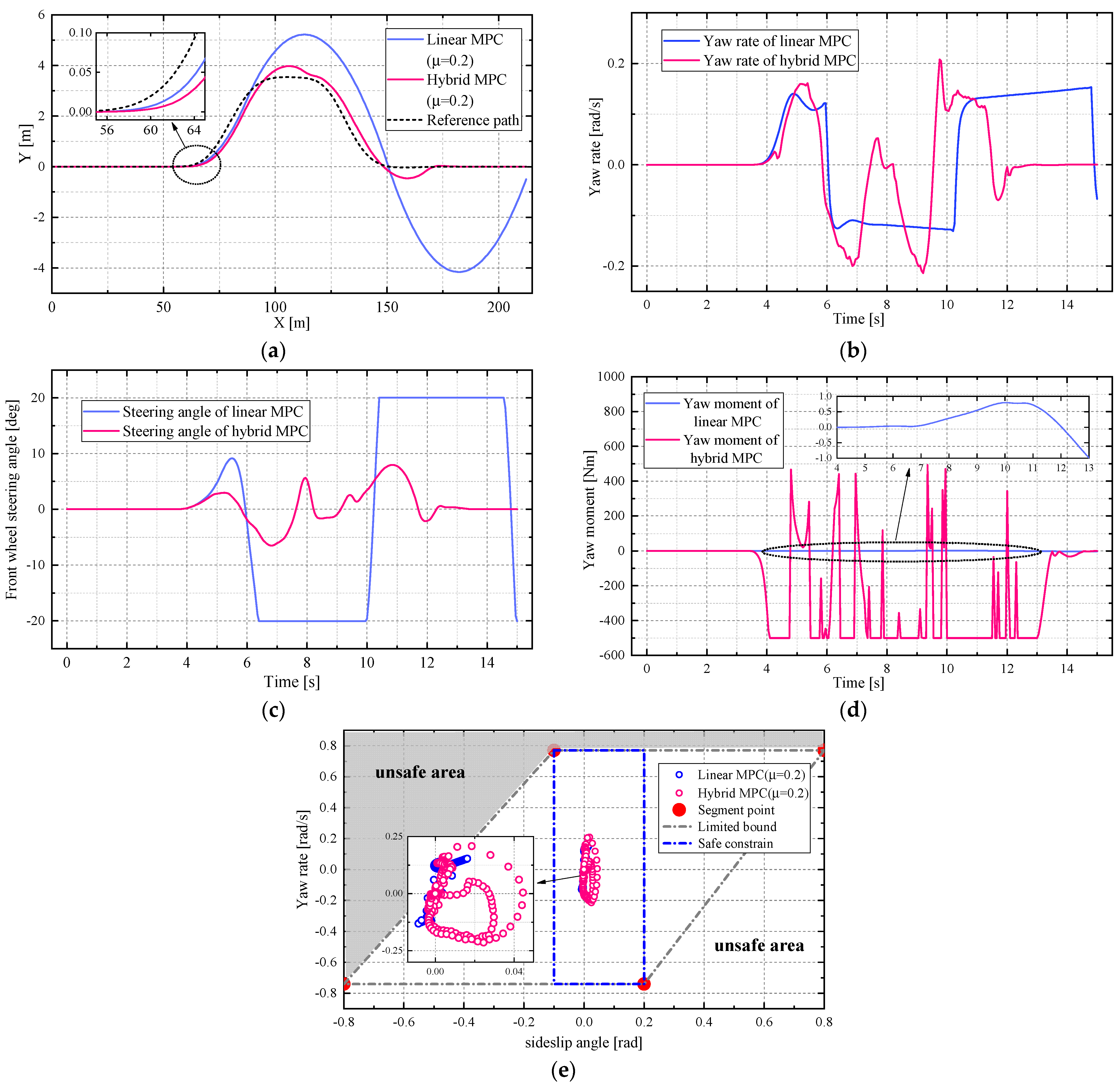
4.1. Simulation in a DLC Scenario

To testify the path tracking the performance of hMPC in the extreme scenario, a maneuver of DLC in low-adhesion and high speed ( v x = 54 km / h ,   μ = 0.2 ) is conducted. The path tracking results are shown in Figure 7, it is obvious that the path tracking error using hMPC controller is smaller than the linear MPC controller as illustrated in Figure 7a, and Table 2 also shows hMPC controller results in smaller RMSE. The computing time radio in Table 2, which is calculated by dividing the real cost time by set simulation time, shows that the linear MPC needs lower computing time than hMPC because that QP is easier to solve than MIQP. Figure 7b illustrates that the control value of the steering angle obtained by linear MPC is larger than hMPC, although the partial enlargement in Figure 7a features faster tracking response by linear MPC, it loses the driving stability in the latter part, which causes a vehicle oscillation. Figure 7b also demonstrates that the vehicle maintains a high yaw rate with a large period. As shown in Figure 7d, the control value of the yaw moment in linear hMPC is larger and fluctuates heavier than the linear MPC. The β - r trajectories are plotted in Figure 7e, which shows the results obtained by both controllers are all in the stable zone, proving that safe constraints can ensure vehicle stability in low-adhesion road conditions. However, the hMPC controller both shows better path tracking performance and can handle the vehicle stability in extreme maneuvers.

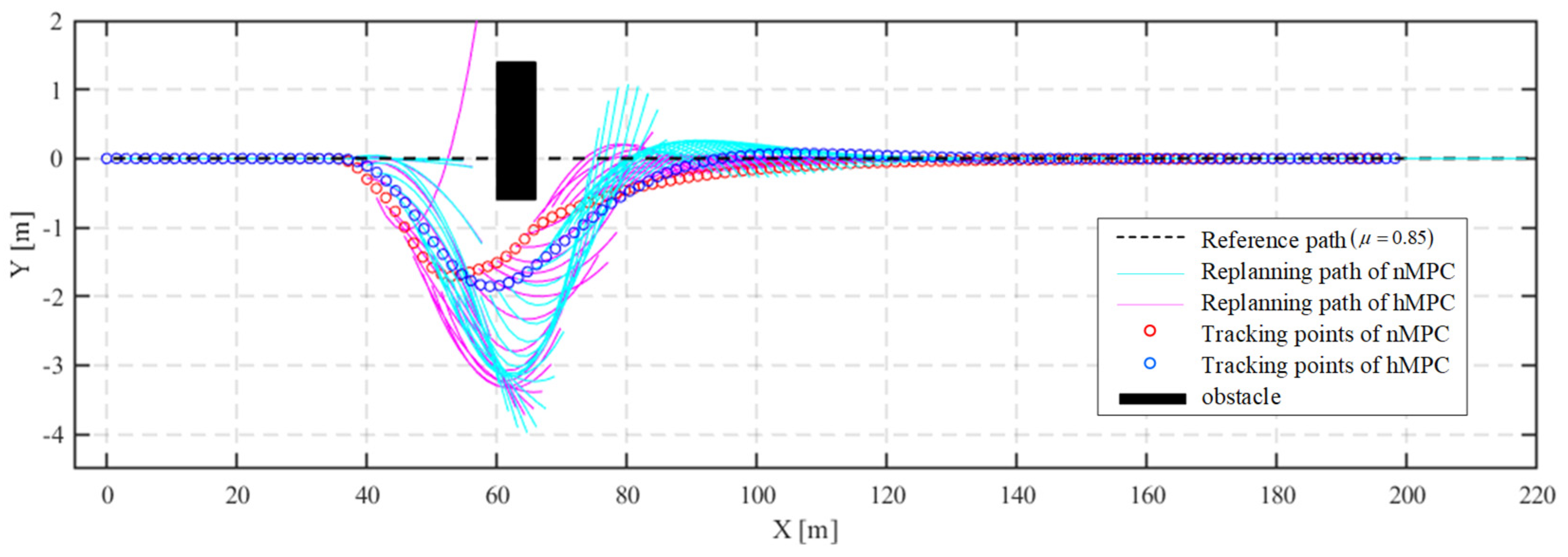
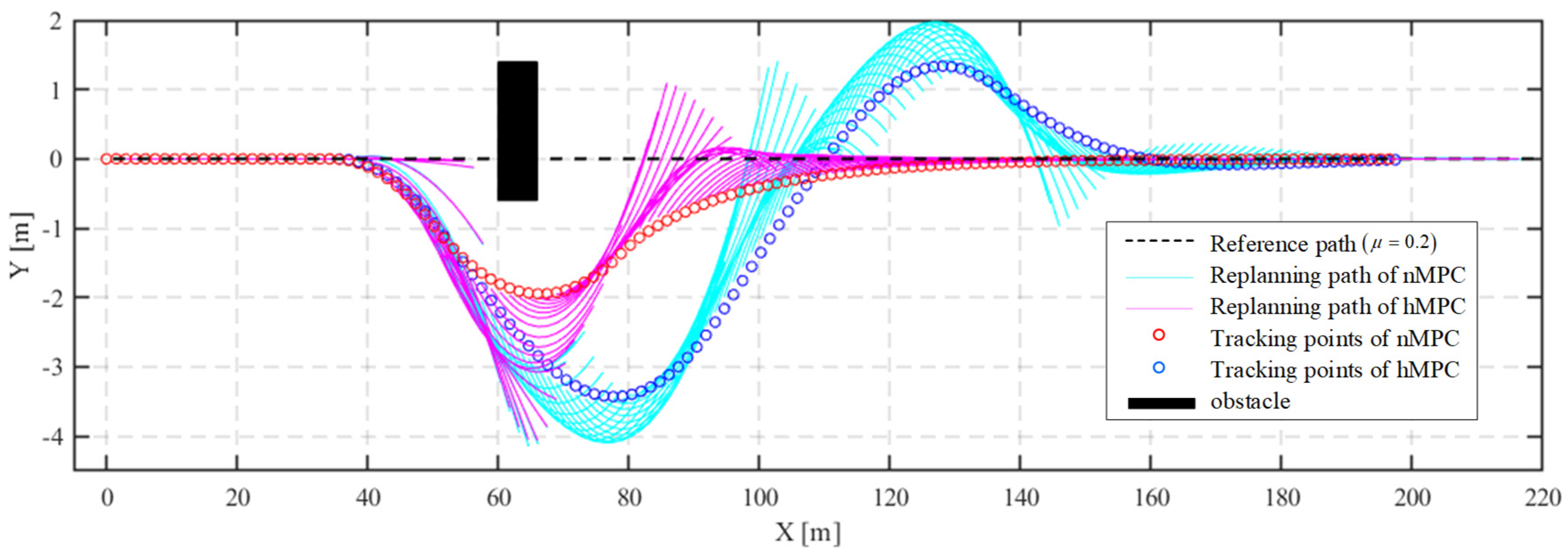
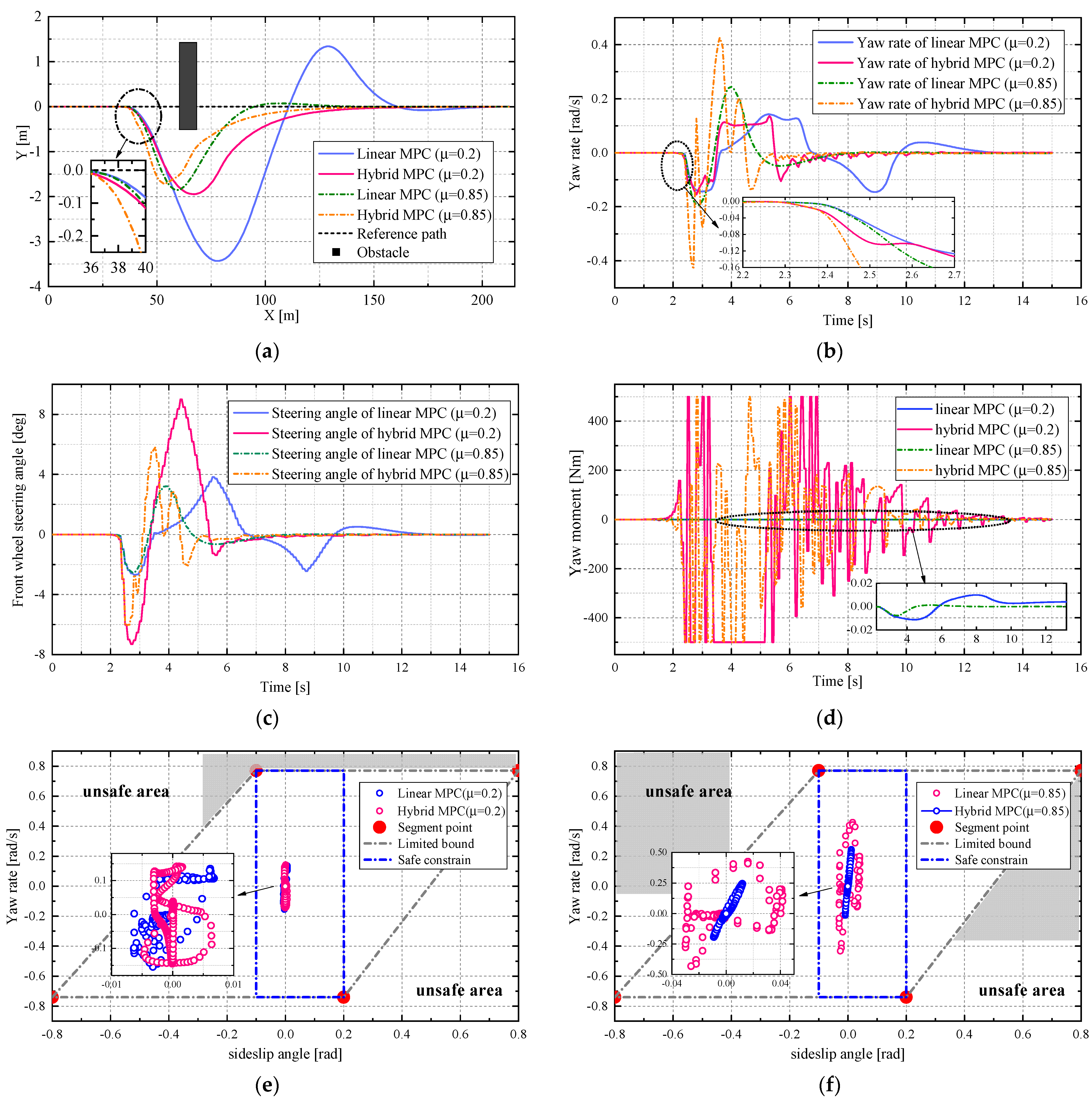
4.2. Simulation in a collIsion Avoidance Scenario

Two different adhesion roads ( μ = 0.2   and   μ = 0.85 ) and path tracking controllers are set to compare and evaluate the performance of the hierarchical controller in a variable collision avoidance scenario at high speed ( v x = 54   km / h ) . The results of path replanning and tracking are shown in Figure 8, Figure 9 and Figure 10a, which illustrates that the path tracking controller using hMPC reduces the risk of instability when drive on a low-adhesion road and effectively accomplishes the collision avoidance compared to the linear MPC. Table 3 presents the smaller RMSE of tracking errors and the higher computing time but not by much in two conditions using hMPC. The interpolation curves illustrated in Figure 8 and Figure 9 are obtained by each step in the simulation, which shows that the nMPC controller can replan a safe path to avoid the obstacle.
In the scenario of μ = 0.2 , the linear MPC controller causes a high amplitude, on the contrary, the hMPC tracks the path smoothly. In the scenario of μ   = 0.85 , as shown in enlargement of Figure 10b, the linear MPC controller responds more slowly than hMPC when the avoidance signal triggers. The additional vehicle parameters comparison is presented in Figure 10c–e. In Figure 10c, the results show that the hMPC controller can immediately respond to the avoidance signal compared to linear MPC. In the scenario of μ   = 0.2 , the yaw rate using hMPC becomes stable at the latter part of the lane while using linear MPC still fluctuates, the same conclusion is reflected in Figure 10d. Figure 10e demonstrates that the additional yaw moment control signal calculated by hMPC is widely utilized in the process of path tracking, but when obtained by the linear MPC is small and cannot improve the control ability.
Figure 10e,f presents the β - r results in two scenarios, which indicate the state trajectories both in the stable zone. In the low-adhesion condition, the β - r trajectories obtained by linear and hybrid MPC show similar distribution. In contrast, the trajectories in the high-adhesion condition simulated by the hybrid MPC show wider distribution than linear MPC but acquire better collision avoidance and tracking effect.

5. Conclusions

A hierarchical predictive-based controller is proposed to improve the extreme autonomous collision avoidance performance of 4IDEV in this paper. The upper controller based on nMPC replans a collision-free path approximated by the polynomial, and the lower controller based on hMPC using the PWA tire model ensures a good performance of path tracking and driving stability in extreme conditions. Moreover, the vehicle lateral stability is analyzed by the phase portrait to gain a stable region. The results of the MATLAB and CarSim co-simulation platform confirm that: (1) In a low-adhesion DLC scenario, compared to the linear MPC method, the proposed hierarchical controller considering the nonlinear characteristics of tires achieves smaller tracking error in extreme road conditions and ensures the vehicle stability; (2) In a low-adhesion collision avoidance scenario, the presented method generates a safe path and results in a faster control response than the linear MPC method when meeting an obstacle, meanwhile, the lateral stability is handled with better tracking performance.
Future work will consider the learning-based method used for planning trajectory optimization.

Author Contributions

Conceptualization, C.L.; Formal analysis, B.W.; Funding acquisition, C.L.; Investigation, Z.T.; Methodology, S.L. and X.G.; Software, B.W., S.L., X.G. and Z.T.; Supervision, C.L.; Validation, B.W.; Visualization, S.L.; Writing—original draft, B.W.; Writing—review & editing, B.W., S.L. and X.G. All authors have read and agreed to the published version of the manuscript.

Funding

This research was funded by the National Natural Science Foundation of China under Grant 51975049.

Institutional Review Board Statement

Not applicable.

Informed Consent Statement

Not applicable.

Conflicts of Interest

The authors declare no conflict of interest.

References

  1. Hang, P.; Chen, X.; Luo, F. LPV/H∞ Controller Design for Path Tracking of Autonomous Ground Vehicles Through Four-Wheel Steering and Direct Yaw-Moment Control. Int. J. Automot. Technol. 2019, 20, 679–691. [Google Scholar] [CrossRef]
  2. Lin, C.; Liang, S.; Chen, J.; Gao, X. A Multi-Objective Optimal Torque Distribution Strategy for Four In-Wheel-Motor Drive Electric Vehicles. IEEE Access 2019, 7, 64627–64640. [Google Scholar] [CrossRef]
  3. Zhao, B.; Xu, N.; Chen, H.; Guo, K.; Huang, Y. Design and Experimental Evaluations on Energy-Efficient Control for 4WIMD-EVs Considering Tire Slip Energy. IEEE Trans. Veh. Technol. 2020, 69, 14631–14644. [Google Scholar] [CrossRef]
  4. Zhang, C.; Chang, B.; Zhang, R.; Wang, R.; Wang, J. Observation of Dynamic State Parameters and Yaw Stability Control of Four-Wheel-Independent-Drive EV. World Electr. Veh. J. 2021, 12, 105. [Google Scholar] [CrossRef]
  5. Huang, Y.; Ding, H.; Zhang, Y.; Wang, H.; Cao, D.; Xu, N.; Hu, C. A Motion Planning and Tracking Framework for Autonomous Vehicles Based on Artificial Potential Field Elaborated Resistance Network Approach. IEEE Trans. Ind. Electron. 2020, 67, 1376–1386. [Google Scholar] [CrossRef]
  6. Lu, B.; He, H.; Yu, H.; Wang, H.; Li, G.; Shi, M.; Cao, D. Hybrid Path Planning Combining Potential Field with Sigmoid Curve for Autonomous Driving. Sensors 2020, 20, 7197. [Google Scholar] [CrossRef] [PubMed]
  7. Wahid, N.; Zamzuri, H.; Amer, N.H.; Dwijotomo, A.; Saruchi, S.A.; Mazlan, S.A. Vehicle collision avoidance motion planning strategy using artificial potential field with adaptive multi-speed scheduler. IET Intell. Transp. Syst. 2020, 14, 1200–1209. [Google Scholar] [CrossRef]
  8. Lim, W.; Lee, S.; Sunwoo, M.; Jo, K. Hierarchical Trajectory Planning of an Autonomous Car Based on the Integration of a Sampling and an Optimization Method. IEEE Trans. Intell. Transp. Syst. 2018, 19, 613–626. [Google Scholar] [CrossRef]
  9. Zhang, X.; Liniger, A.; Borrelli, F. Optimization-Based Collision Avoidance. IEEE Trans. Control. Syst. Technol. 2021, 29, 972–983. [Google Scholar] [CrossRef] [Green Version]
  10. Liu, J.; Jayakumar, P.; Stein, J.L.; Ersal, T. Combined Speed and Steering Control in High-Speed Autonomous Ground Vehicles for Obstacle Avoidance Using Model Predictive Control. IEEE Trans. Veh. Technol. 2017, 66, 8746–8763. [Google Scholar] [CrossRef]
  11. Chen, L.; Ma, Y.; Zhang, Y.; Liu, J. Obstacle Avoidance and Multitarget Tracking of a Super Redundant Modular Manipulator Based on Bezier Curve and Particle Swarm Optimization. Chin. J. Mech. Eng. 2020, 33, 1–19. [Google Scholar] [CrossRef]
  12. Li, H.; Luo, Y.; Wu, J. Collision-Free Path Planning for Intelligent Vehicles Based on Bézier Curve. IEEE Access 2019, 7, 123334–123340. [Google Scholar] [CrossRef]
  13. Huang, C.; Huang, H.; Hang, P.; Gao, H.; Wu, J.; Huang, Z.; Lv, C. Personalized Trajectory Planning and Control of Lane-Change Maneuvers for Autonomous Driving. IEEE Trans. Veh. Technol. 2021, 70, 5511–5523. [Google Scholar] [CrossRef]
  14. Ding, W.; Zhang, L.; Chen, J.; Shen, S. Safe Trajectory Generation for Complex Urban Environments Using Spatio-Temporal Semantic Corridor. IEEE Robot. Autom. Lett. 2019, 4, 2997–3004. [Google Scholar] [CrossRef] [Green Version]
  15. Wang, H.; Lu, B.; Li, J.; Liu, T.; Xing, Y.; Lv, C.; Cao, D.; Li, J.; Zhang, J.; Hashemi, E. Risk Assessment and Mitigation in Local Path Planning for Autonomous Vehicles With LSTM Based Predictive Model. IEEE Trans. Autom. Sci. Eng. 2021, 1–12. [Google Scholar] [CrossRef]
  16. Hang, P.; Lv, C.; Huang, C.; Cai, J.; Hu, Z.; Xing, Y. An Integrated Framework of Decision Making and Motion Planning for Autonomous Vehicles Considering Social Behaviors. IEEE Trans. Veh. Technol. 2020, 69, 14458–14469. [Google Scholar] [CrossRef]
  17. Chen, Y.; Hu, C.; Wang, J. Motion Planning with Velocity Prediction and Composite Nonlinear Feedback Tracking Control for Lane-Change Strategy of Autonomous Vehicles. IEEE Trans. Intell. Veh. 2020, 5, 63–74. [Google Scholar] [CrossRef]
  18. Wang, Y.; Shao, Q.; Zhou, J.; Zheng, H.; Chen, H. Longitudinal and lateral control of autonomous vehicles in multi-vehicle driving environments. IET Intell. Transp. Syst. 2020, 14, 924–935. [Google Scholar] [CrossRef]
  19. Zheng, L.; Zeng, P.; Yang, W.; Li, Y.; Zhan, Z. Bézier curve-based trajectory planning for autonomous vehicles with collision avoidance. IET Intell. Transp. Syst. 2020, 14, 1882–1891. [Google Scholar] [CrossRef]
  20. Hang, P.; Han, Y.; Chen, X.; Zhang, B. Design of an Active Collision Avoidance System for a 4WIS-4WID Electric Vehicle. In Proceedings of the 5th IFAC Conference on Engine and Powertrain Control, Simulation and Modeling, Changchun, China, 20–22 September 2018; pp. 771–777. [Google Scholar]
  21. Hang, P.; Xia, X.; Chen, X. Handling Stability Advancement With 4WS and DYC Coordinated Control: A Gain-Scheduled Robust Control Approach. IEEE Trans. Veh. Technol. 2021, 70, 3164–3174. [Google Scholar] [CrossRef]
  22. Li, X.; Xu, N.; Guo, K.; Huang, Y. An adaptive SMC controller for EVs with four IWMs handling and stability enhancement based on a stability index. Veh. Syst. Dyn. 2020, 59, 1509–1532. [Google Scholar] [CrossRef]
  23. Yang, K.; Dong, D.; Ma, C.; Tian, Z.; Chang, Y.; Wang, G. Stability Control for Electric Vehicles with Four In-Wheel-Motors Based on Sideslip Angle. World Electr. Veh. J. 2021, 12, 42. [Google Scholar] [CrossRef]
  24. He, Z.; Nie, L.; Yin, Z.; Huang, S. A Two-Layer Controller for Lateral Path Tracking Control of Autonomous Vehicles. Sensors 2020, 20, 3689. [Google Scholar] [CrossRef]
  25. Tang, L.; Yan, F.; Zou, B.; Wang, K.; Lv, C. An Improved Kinematic Model Predictive Control for High-Speed Path Tracking of Autonomous Vehicles. IEEE Access 2020, 8, 51400–51413. [Google Scholar] [CrossRef]
  26. Choi, M.; Choi, S.B. Model Predictive Control for Vehicle Yaw Stability with Practical Concerns. IEEE Trans. Veh. Technol. 2014, 63, 3539–3548. [Google Scholar] [CrossRef]
  27. Li, S.E.; Chen, H.; Li, R.; Liu, Z.; Wang, Z.; Xin, Z. Predictive lateral control to stabilise highly automated vehicles at tire-road friction limits. Veh. Syst. Dyn. 2020, 58, 768–786. [Google Scholar] [CrossRef]
  28. Di Cairano, S.; Tseng, H.E.; Bernardini, D.; Bemporad, A. Vehicle Yaw Stability Control by Coordinated Active Front Steering and Differential Braking in the Tire Sideslip Angles Domain. IEEE Trans. Control. Syst. Technol. 2012, 21, 1236–1248. [Google Scholar] [CrossRef]
  29. Ataei, M.; Khajepour, A.; Jeon, S. Model Predictive Control for integrated lateral stability, traction/braking control, and rollover prevention of electric vehicles. Veh. Syst. Dyn. 2019, 58, 49–73. [Google Scholar] [CrossRef]
  30. Yuan, K.; Shu, H.; Huang, Y.; Zhang, Y.; Khajepour, A.; Zhang, L. Mixed local motion planning and tracking control framework for autonomous vehicles based on model predictive control. IET Intell. Transp. Syst. 2019, 13, 950–959. [Google Scholar] [CrossRef]
  31. Ji, J.; Khajepour, A.; Melek, W.W.; Huang, Y. Path Planning and Tracking for Vehicle Collision Avoidance Based on Model Predictive Control With Multiconstraints. IEEE Trans. Veh. Technol. 2017, 66, 952–964. [Google Scholar] [CrossRef]
  32. Sazgar, H.; Azadi, S.; Kazemi, R. Trajectory planning and combined control design for critical high-speed lane change manoeuvres. Proc. Inst. Mech. Eng. Part D J. Automob. Eng. 2019, 234, 823–839. [Google Scholar] [CrossRef]
  33. Gao, Y.; Gordon, T.; Lidberg, M. Optimal control of brakes and steering for autonomous collision avoidance using modified Hamiltonian algorithm. Veh. Syst. Dyn. 2019, 57, 1224–1240. [Google Scholar] [CrossRef]
  34. Liu, J.; Jayakumar, P.; Stein, J.L.; Ersal, T. Improving the robustness of an MPC-based obstacle avoidance algorithm to parametric uncertainty using worst-case scenarios. Veh. Syst. Dyn. 2019, 57, 874–913. [Google Scholar] [CrossRef]
  35. Borri, A.; Bianchi, D.; Di Benedetto, M.; Di Gennaro, S. Optimal workload actuator balancing and dynamic reference generation in active vehicle control. J. Frankl. Inst. 2017, 354, 1722–1740. [Google Scholar] [CrossRef]
  36. Bianchi, D.; Borri, A.; Toledo, B.C.; Di Benedetto, M.D.; Di Gennaro, S. Smart management of actuator saturation in integrated vehicle control. In Proceedings of the 2011 5th IEEE Conference on Decision and Control and European Control Conference, Orlando, FL, USA, 12–15 December 2011; pp. 2529–2534. [Google Scholar]
  37. Bobier, C.G.; Gerdes, J.C. Staying within the nullcline boundary for vehicle envelope control using a sliding surface. Veh. Syst. Dyn. 2013, 51, 199–217. [Google Scholar] [CrossRef]
  38. Alberto Bemporad, M.M. Control of systems integrating logic, dynamics, and constraints. Automatica 1999, 39, 407–427. [Google Scholar] [CrossRef]
  39. Torrisi, F.; Bemporad, A. HYSDEL—A Tool for Generating Computational Hybrid Models for Analysis and Synthesis Problems. IEEE Trans. Control. Syst. Technol. 2004, 12, 235–249. [Google Scholar] [CrossRef]
Figure 1. PWA approximation of tire magic formula.
Wevj 12 00192 g001
Figure 2. 2DOF bicycle model.
Wevj 12 00192 g002
Figure 3. Full-wheel drive vehicle model.
Wevj 12 00192 g003
Figure 4. (ad) shows the phase portrait with the front wheel steering angle of 0 rad, 0.1 rad, 0.25 rad, 0.35 rad, respectively. The red dotted line represents the boundary of different regions; the blue dotted line represents the position of saddle points.
Wevj 12 00192 g004
Figure 5. Limited bound and safe constrain.
Wevj 12 00192 g005
Figure 6. The hierarchical control scheme.
Wevj 12 00192 g006
Figure 7. Simulation results in low-adhesion DLC scenario. (a) Path tracking performance; (b) Yaw rate comparison; (c) Steering angle comparison; (d) Yaw moment comparison. (e) State trajectories of sideslip angle and yaw rate.
Wevj 12 00192 g007
Figure 8. Path replanning and collision avoidance on the road of μ = 0.85 .
Wevj 12 00192 g008
Figure 9. Path replanning and collision avoidance on the road of μ = 0.2 .
Wevj 12 00192 g009
Figure 10. Simulation results in the variable collision avoidance scenario. (a) Path tracking performance; (b) Yaw rate comparison; (c) Steering angle comparison; (d) Yaw moment comparison; (e) State trajectories in low-adhesion condition; (f) State trajectories in high-adhesion condition.
Wevj 12 00192 g010
Table 1. Vehicle simulation parameters.
ParameterValueUnitParameterValueUnit
l f 1.015m m 1270kg
l r 1.885m g 9.8m/s2
v x 15m/s I z 1536.7Kg·m2
Table 2. Comparison of tracking errors and computing time of two methods.
Path Tracking ControllerRMSE of Tracking ErrorsComputing Time Radio
Hybrid MPC0.200678.42104
Linear MPC1.369477.52817
Table 3. Comparison of tracking errors and computing time of two methods.
Path Tracking ControllerRMSE of Tracking ErrorComputing Time Radio
Hybrid MPC ( μ = 0.85 )0.4492527.8171
Hybrid MPC ( μ = 0.2 )0.5864425.2747
Linear MPC ( μ = 0.85 )0.4985026.5447
Linear MPC ( μ = 0.2 )1.0905323.4518
Publisher’s Note: MDPI stays neutral with regard to jurisdictional claims in published maps and institutional affiliations.

