Core Loss Analysis and Modeling of a Magnetic Coupling System in WPT for EVs

Abstract

The magnetic core is an important part of the magnetic coupling system in wireless power transmission (WPT) for EVs. It helps to increase the coupling coefficient and reduce magnetic field leakage. However, it also brings additional core loss. While the traditional core loss model cannot be used directly due to the uneven distribution of the magnetic flux density, this paper focuses on the flux density distribution in the disk core of a WPT system. Based on a finite element analysis (FEA) simulation and a theoretical magnetic flux density distribution analysis, a mathematical model of magnetic flux density distribution is built, which is regarded as a quadratic function. Through this model, the flux density distribution can be calculated by the electrical and mechanical specifications of the magnetic coupling system. Combining the model of flux density distribution, the disk core loss model of the WPT system is proposed—the idea of which is dividing the disk core into several circle sheets firstly, and then summing the core loss of all circle sheets. Finally, the FEA simulation results verify the proposed model as being correct and flexible.

1. Introduction

To ease the shortage of fossil energy and the problem of environmental pollution, electric vehicles have been adopted in recent years [1,2]. Traditionally, contact-type chargers are used in electric vehicles. But this power transmission method needs charge wires and sockets, which may cause electric sparks and decrease safety levels. People hope to find a convenient, safe and highly reliable power transmission method [3]. Compared to the traditional contact-type power transmission method, wireless power transmission (WPT) technology can not only avoid the electric sparks caused by physical contact, but also be greatly convenient for users [4,5,6]. Now, WPT technology for electric vehicles has attracted a lot of attention from all over the world [7,8,9,10,11,12,13].

The magnetic coupling system is the most important part for realizing wireless power transmission. Usually, the distance between the transmitter and the receiver is relatively large in the application of WPT for EVs. In order to strengthen the coupling coefficient between the transmitter and the receiver to improve the transmission power and efficiency and to reduce magnetic field leakage, magnetic cores are adopted in WPT system [14]. However, the magnetic cores may bring additional core loss and reduce the efficiency of the prototype [15].

To evaluate and optimize the core loss of the magnetic coupling system, it is necessary to build a core loss model. Currently, the Steinmetz formula is widely used as a core loss model, in which the parameters are obtained by measurement. In core loss measurement, the one-winding method, two-winding method and calorimetric method are widely used. In [16,17], the core loss is obtained by calculating the product of the measured voltage and current across the magnetic component. However, the core loss measured by this method includes both the winding loss and the core loss, and the individual core loss cannot be obtained. This method is suitable for applications where the core loss is much greater than the winding loss, such as in ferrite transformers. But in WPT applications, the winding loss represents a large amount of the whole loss in the magnetic coupling system. In [18,19,20], the two-winding method is adopted to calculate the product of the measured current of the power winding and the measured voltage of the auxiliary winding to obtain the core loss of the magnetic component. This measured loss does not include the winding loss of the component and the individual core loss can be obtained. However, this method requires the coupling coefficient between the two windings to be high enough (close to 1). Additionally, the coupling coefficient of the WPT system is relatively small (usually less than 0.7) [21,22]—as a result, the two-winding method cannot be used to measure the core loss of the WPT system. In [23,24,25], the calorimetric method was discussed. In this method, the magnetic component is put into a closed container, and then the heat generated by the voltage and current excitation can be measured according to the temperature rise; finally, the core loss of the magnetic component can be calculated. As well as the one-winding method, the core loss measured by this method not only includes the core loss but also the winding loss, and it is suitable for applications where the core loss is much greater than the winding loss.

Moreover, the Steinmetz formula can only calculate the core loss at certain frequencies and magnetic flux densities of a magnetic component. The magnetic flux density in the ferrite inductor and the transformer of the switching mode power supply (the air gap is generally small and the coupling coefficient is close to 1) is basically uniform; therefore, the Steinmetz formula calculation result can effectively characterize the core loss of inductors and transformers [26,27]. However, for the WPT system, the magnetic core adopts a disk-shaped structure, and the distance between the two disk cores is relatively large (for example, the air gap is 5 cm). As a result, the coupling coefficient of the WPT system is usually low and the magnetic field leakage is serious [21,22]. Therefore, the magnetic flux density inside the disk core is uneven. The Steinmetz formula cannot be used directly for core loss calculation, because of its non-linear characteristic. In this situation, finite element analysis (FEA) simulation can be adopted for WPT core loss calculation. However, it takes a lot of time—especially in 3D FEA simulation [28]. This paper focuses on the magnetic flux density distribution in the disk core of the WPT system. Based on simulations and theoretical analysis, the theory model of magnetic flux density distribution can be built, and then the core loss model can be proposed. The core loss of the disk core of the WPT system can be easily obtained by the proposed core loss model, which can save time and calculation resources compared to FEA simulation.

The sections of this paper are organized as follows: Section 2 analyzes the distribution of magnetic flux density in the disk core by FEA simulation. It reveals that the distribution of the magnetic flux density in the disk core is uneven. Section 3 establishes the mathematical model of the distribution of the magnetic flux density in the disk core, and based on the Steinmetz formula, the disk core loss model of the magnetic coupling system is proposed. Section 4 verifies the accuracy of the disk core loss calculation method through FEA simulation, and conclusions are drawn in Section 5.

2. The Distribution of Magnetic Flux Density in the Disk Core

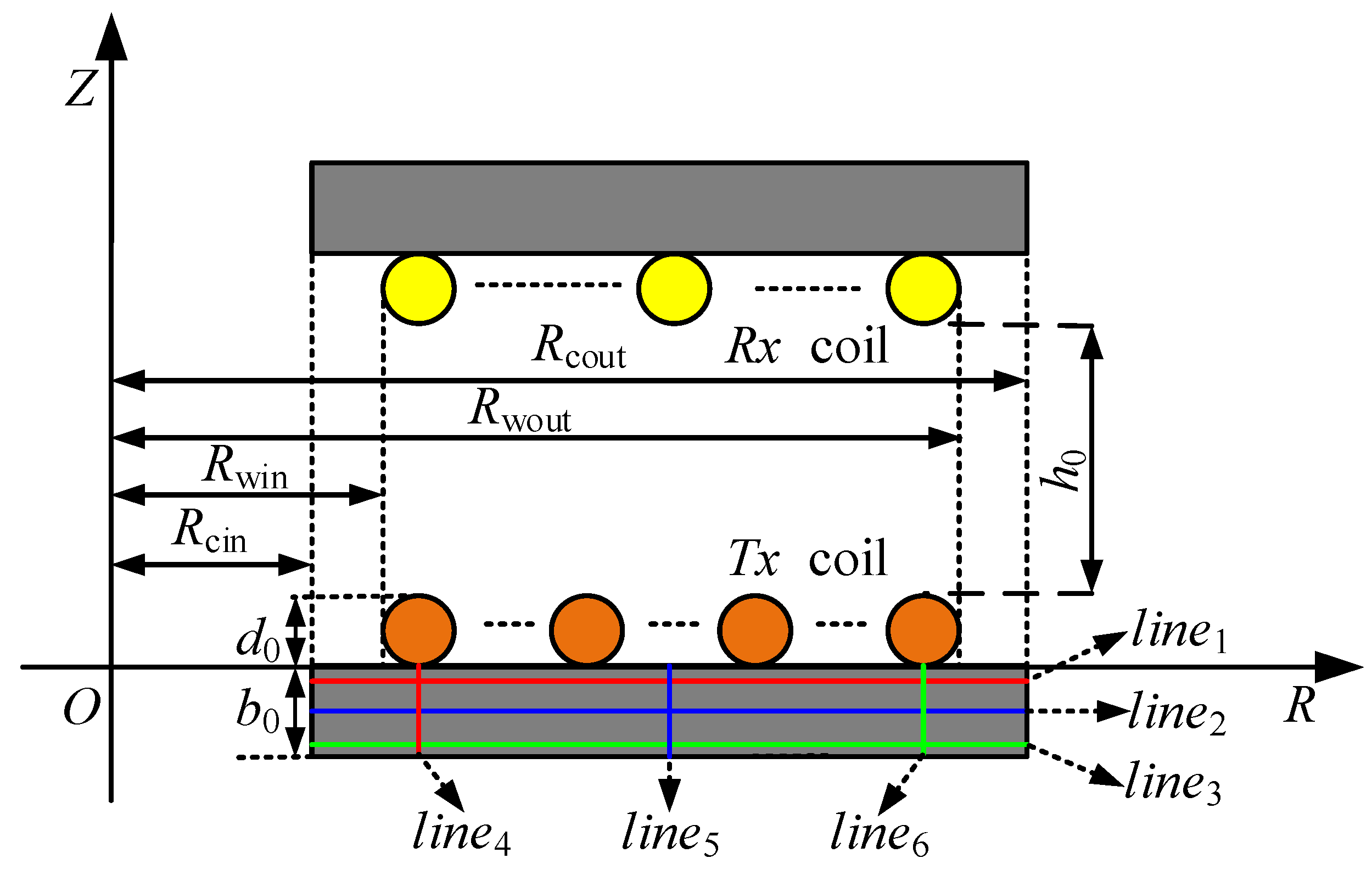
Usually, the uniformly distributed planar spiral winding structure is used in WPT magnetic coupling systems, while a disk structure is used as the magnetic core structure. The simulation model of the magnetic coupling system with the disk core is established in Figure 1, and the parameters and setup of the simulation model are shown in

Table 1. The parameters and setup of magnetic coupling system.

Magnetic Coupling System Model Parameters	Parameters and Setup
The inner and outer radius of the winding	Rwin = 100 mm	Rwout = 250 mm
The inner and outer radius of the core	Rcin = 70 mm	Rcout = 280 mm
Coil diameter and core thickness	d0 = 4.2 mm	b0 = 100 mm
Turns of transmitter winding and receiver winding	Np = 23 turns	Ns = 18 turns
Transmitter winding current and receiver winding current	Ip = 12 A	Is = 18 A
Core material	Philips-3C96
Boundary conditions	Balloon border
The transmission distance between coils	h0 = 50 mm

.

Through FEA simulation, the plot of the magnetic flux density inside the magnetic core could be acquired, as shown in Figure 2. Additionally, the curve of the magnetic flux density inside the transmitter core versus R-axis and Z-axis position could be obtained as shown in Figure 3. Where the transmitter winding current I_p = 12 A, the receiver winding current I_s = 18 A and the phase-shift = 0°.

It can be seen from Figure 2 that the distribution of magnetic flux density inside the magnetic core was uneven. The flux density was approximately zero at the boundary of the magnetic core, and there was a maximum at the center.

Figure 3a shows that the magnetic flux density under same Z-axis was basically consistent (at different R-axis positions); therefore, the flux density of each circle sheet was nearly the same. The tendency of Figure 3b was similar with a quadratic function. In this situation, the average magnetic flux density cannot be directly used to calculate the overall core loss due to the non-linear core loss characteristics.

3. Analysis and Modeling of Core Loss

3.1. Modeling of Magnetic Flux Density Distribution

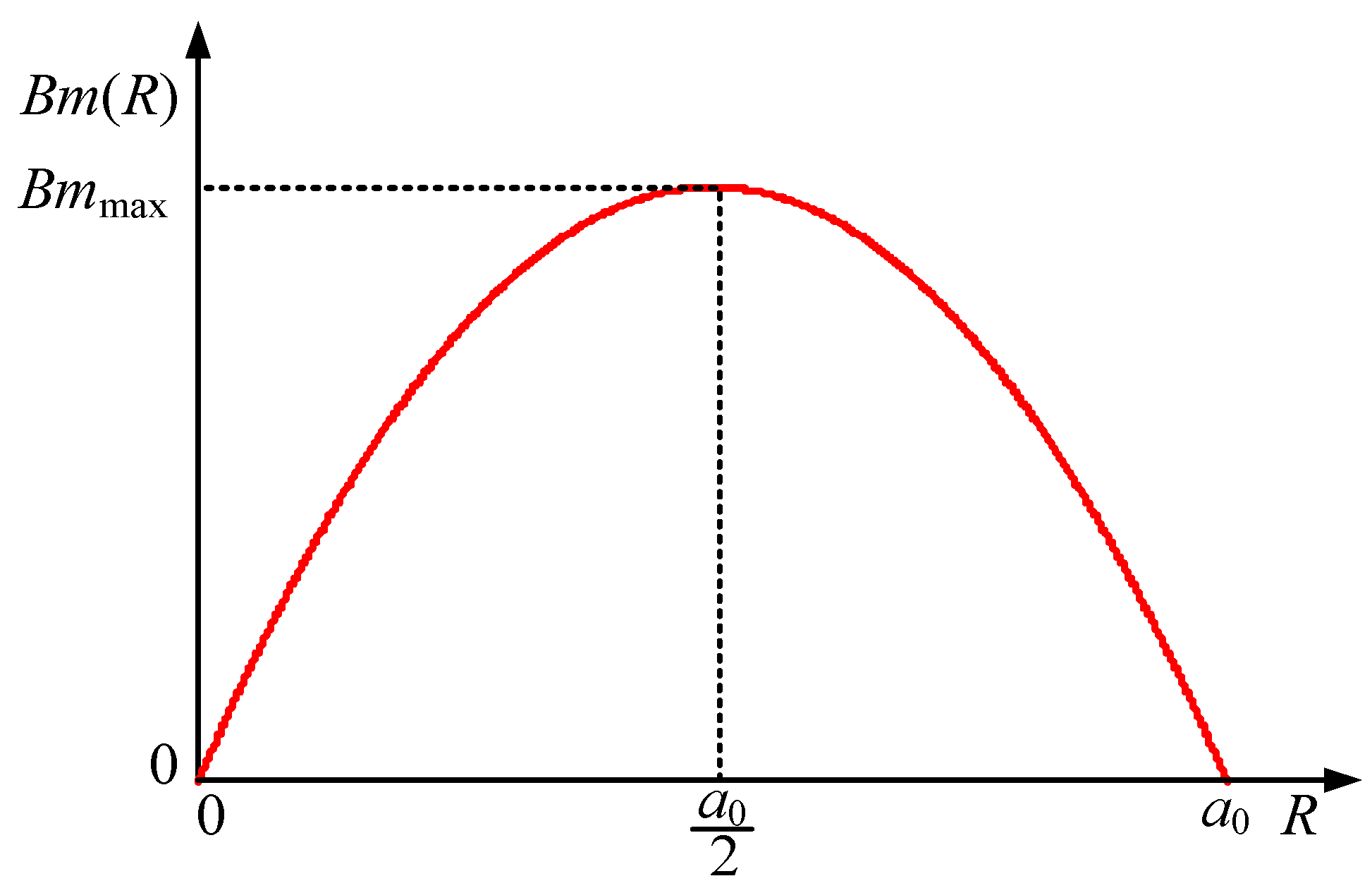
In order to simplify the distribution of magnetic flux density in Figure 3, the magnetic flux density inside the disk core was regarded as the same at different Z-axis positions while varying as different R-axis positions. In addition, the magnetic flux density at both the inner radius and the outer radius of the core was considered to be zero. Hence, a quadratic function distribution along the R-axis is presented. The simplified flux density distribution inside the disk core is shown in Figure 4.

Therefore, the simplified magnetic flux density distribution inside the disk core can be expressed as:

$$Bm(R,B{m}_{\max })=\frac{-4B{m}_{\max }}{a_0{}^2}{R}^2+\frac{4B{m}_{\max }}{a_0}R$$

(1)

3.2. Theoretical Calculation Method of Magnetic Flux Density Model Parameters

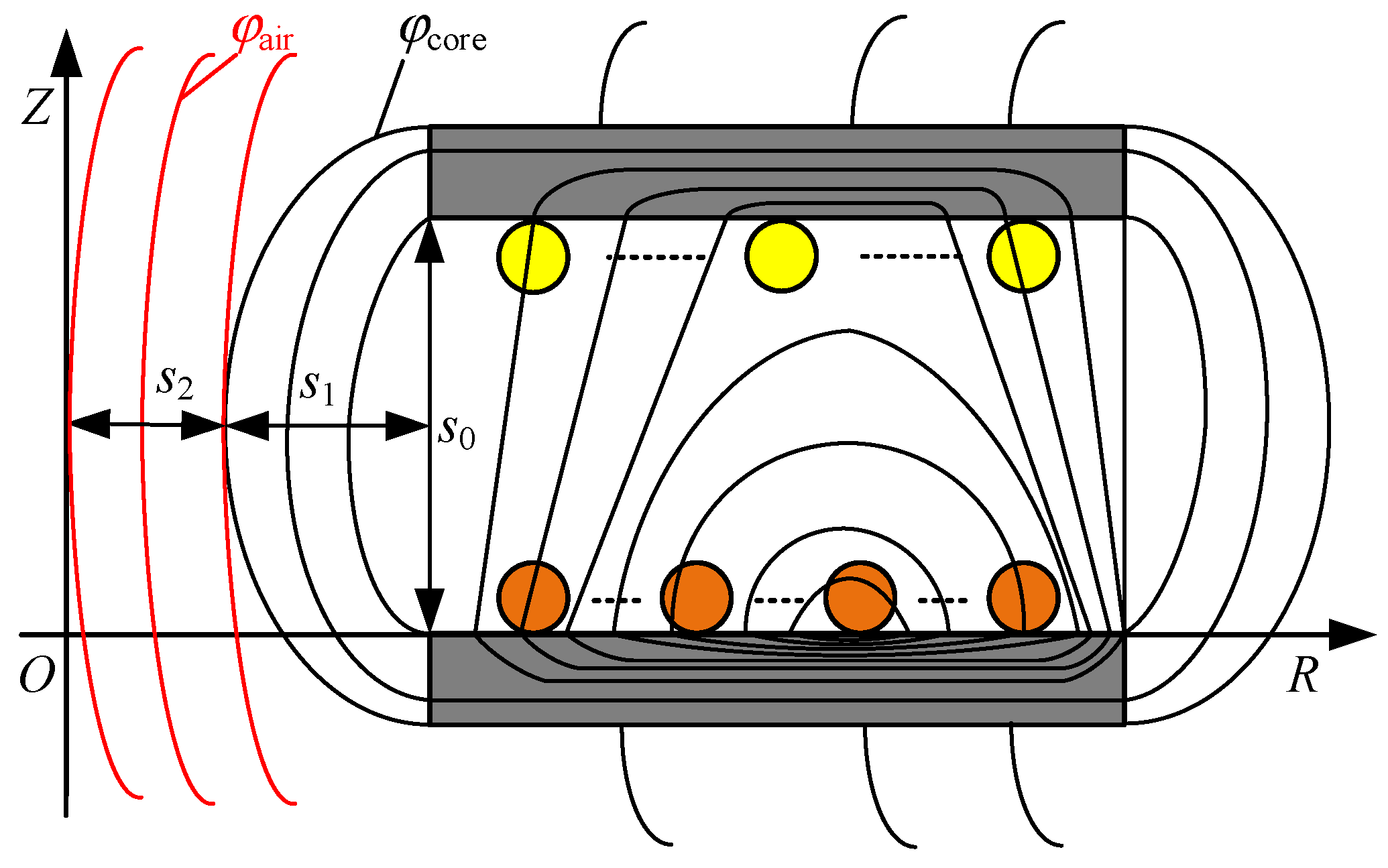
When the Bm_max in Formula (1) is determined, the magnetic flux density distribution inside the disk core can be obtained. However, Bm_max needs to be determined by the magnetic field distribution characteristics of the magnetic coupling system. The magnetic-field line distribution schematic diagram of the magnetic coupling system is shown in Figure 5, where the air gap diffusion effect exists at the inner radius and the outer radius of the magnetic core and the air gap diffusion flux loop is approximately a semicircle [29].

It can be seen from Figure 5 that the flux linkage of the magnetic coupling system mainly includes two parts: One part of the flux linkage φ_core is formed by the magnetic core and air closure and the other φ_air is formed by the air closure. Where s₀ is the distance between the two magnetic cores, s₁ is the distance between the outer edge of the air gap diffusion magnetic flux and the inner radius of the magnetic core, and s₂ is the distance between the outer edge of the air gap diffusion magnetic flux and the center of the winding. The expression of each parameter is:

$$\{\begin{array}{l}{s}_0=h_0+2d_0\\ s_1=\frac{s_0}{2}=\frac{h_0}{2}+d_0\\ s_2=R_{\mathrm{cin}}-s_1=R_{\mathrm{cin}}-\frac{h_0}{2}-d_0\end{array}$$

(2)

It is assumed that the phase-shift of the transmitter winding current ahead of the receiver winding current is θ_p and that the initial phase angle of the receiver winding current is zero, according to the constant-linkage theorem on the transmitter:

$$L_{\mathrm{p}}{I}_{\mathrm{p}}\cos {\theta }_{\mathrm{p}}+M{I}_{\mathrm{s}}+\mathrm{j}{L}_{\mathrm{p}}{I}_{\mathrm{p}}\sin {\theta }_{\mathrm{p}}={\phi }_{1\mathrm{core}}+{\phi }_{1\mathrm{air}}$$

(3)

where φ_1core is the flux linkage formed by the magnetic core and air closure and φ_1air is the flux linkage formed by the air closure on the transmitter.

The flux linkage φ_1core formed by the magnetic core and air closure on the transmitter can be expressed as:

$${\phi }_{1\mathrm{core}}(B{m}_{1\max })={\displaystyle \sum _{i=1}^{N_{\mathrm{p}}}2\mathsf{\pi }{b}_0(R_1(i)+R_{\mathrm{cin}})Bm(R_1(i),B{m}_{1\max })}$$

(4)

where R₁(i) is the relative position of the i-th turn coil center of the transmitter winding, the expression is:

$$R_1(i)=R_{\mathrm{win}}-R_{\mathrm{cin}}+\frac{d_0}{2}+\frac{w_0-d_0}{N_{\mathrm{p}}-1}(i-1)$$

(5)

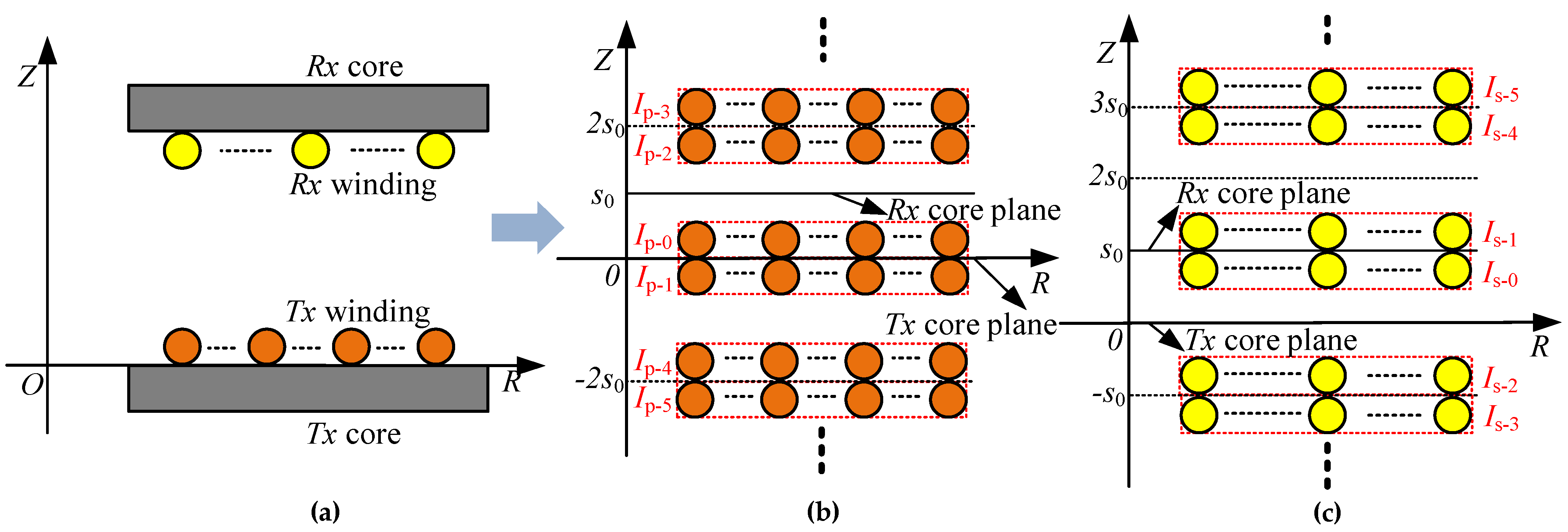
For flux linkage φ_1air formed by the air closure in the s₂ area, this paper ignored the influence of the core thickness and adopted the magnetic-field distribution of the method of images model to obtain the magnetic-field distribution of the magnetic coupling system. The equivalent model of the method of images was established as shown in Figure 6.

The transmitter winding source current group with the current amplitude I_p-0 generates a primary mirror current group with the current amplitude I_p-1 under the action of the transmitter core; the source current and the primary mirror current group will generate a secondary mirror current group with the current amplitude of I_p-2 and a third mirror current group with the current amplitude of I_p-3 under the action of the receiver core, and the second mirror current group and the third mirror current group will generate a fourth mirror current group and a fifth mirror current group under the action of the transmitter core. Similarly, the alternating reflections of the two magnetic core planes produce an infinite set of mirror current groups. In the same way, for the receiver winding current, the alternating reflections of the two magnetic core planes also produce an infinite set of mirror current groups.

In [30], through 2D FEA simulation, it is found that the ratio of the mirror current I_m to the source current I_o is a function with the core plane width, coil diameter and transmission distance:

$$\gamma =\frac{I_{\mathrm{m}}}{I_{\mathrm{o}}}\cong 1-{\mathrm{e}}^{-w_0-\frac{2d_0}{{\alpha }_{2}y}}$$

(6)

where w₀ and d₀ are the core plane width and coil diameter, respectively; y is the vertical position of the magnetic-field test.

It is assumed that the current amplitude of the k-th mirror current group of the transmitter winding current and the receiver winding current obtained according to Formula (6) are I_p-k and I_s-k, respectively. When the thickness of the magnetic core is ignored and the plane of the transmitter core is Z = 0, the axial height of each transmitter mirror current group and receiver mirror current group can be expressed as:

$$h_{I_{\mathrm{p}-\mathrm{k}}}=\{\begin{array}{l}\left\{h_{I_{\mathrm{p}-0}},h_{I_{\mathrm{p}-2}},h_{I_{\mathrm{p}-4}},\dots \dots \right\}=\left\{ \frac{d_0}{2},2s_0-\frac{d_0}{2},-(2s_0-\frac{d_0}{2}),\dots \dots \right\}\\ \left\{h_{I_{\mathrm{p}-1}},h_{I_{\mathrm{p}-3}},h_{I_{\mathrm{p}-5}},\dots \dots \right\}=\left\{-\frac{d_0}{2},2s_0+\frac{d_0}{2},-(2s_0+\frac{d_0}{2}),\dots \dots \right\}\end{array}$$

(7)

$$h_{I_{\mathrm{s}-\mathrm{k}}}=\{\begin{array}{c}\left\{h_{I_{\mathrm{s}-0}},h_{I_{\mathrm{s}-2}},h_{I_{\mathrm{s}-4}},\dots \dots \right\}=\left\{s_0-\frac{d_0}{2},-(s_0-\frac{d_0}{2}),3s_0-\frac{d_0}{2},\dots \dots \right\}\\ \left\{h_{I_{\mathrm{s}-1}},h_{I_{\mathrm{s}-3}},h_{I_{\mathrm{s}-5}},\dots \dots \right\}=\left\{s_0+\frac{d_0}{2},-(s_0+\frac{d_0}{2}),3s_0+\frac{d_0}{2},\dots \dots \right\}\end{array}$$

(8)

The position parameters of the i-th turn transmitter mirror current and the receiver mirror current of the k-th group of current can be expressed as:

$$\{\begin{array}{c}{R}_1(k,i)=R_1(i)\\ z_1(k,i)=h_{I_{\mathrm{p}-\mathrm{k}}}\end{array}$$

(9)

$$\{\begin{array}{c}{R}_2(k,i)=R_2(i)\\ z_2(k,i)=h_{I_{\mathrm{s}-\mathrm{k}}}\end{array}$$

(10)

where there is a load coil at the radial distance s₂ and the axial height s₀/2, taking the i-th turn of the k-th transmitter mirror current group and the receiver mirror current group, as an example. According to the method of magnetic vector potential, the mutual inductance magnetic flux generated in the load coil can be expressed as:

$$\{\begin{array}{l}{\varphi }_{1\mathrm{air}\_\mathrm{unit}}(k,i)={\displaystyle \underset{l_3}{\oint }\stackrel{\rightharpoonup }{A_1}(k,i)·d\stackrel{\rightharpoonup }{l_3}=}\frac{{\mu }_0·I_{\mathrm{p}-\mathrm{k}}(\cos {\theta }_{\mathrm{p}}+\mathrm{j}\sin {\theta }_{\mathrm{p}})}{4\pi }{\displaystyle \underset{l_3}{\oint }{\displaystyle \underset{l_1}{\oint }\frac{d\stackrel{\rightharpoonup }{l_1}(k,i)·d\stackrel{\rightharpoonup }{l_3}}{R(k,i)}}}\\ {\varphi }_{2\mathrm{air}\_\mathrm{unit}}(k,i)={\displaystyle \underset{l_3}{\oint }\stackrel{\rightharpoonup }{A_2}(k,i)·d\stackrel{\rightharpoonup }{l_2}=}\frac{{\mu }_0·I_{\mathrm{s}-\mathrm{k}}}{4\pi }{\displaystyle \underset{l_3}{\oint }{\displaystyle \underset{l_2}{\oint }\frac{d\stackrel{\rightharpoonup }{l_2}(k,i)·d\stackrel{\rightharpoonup }{l_3}}{R^{\prime }(k,i)}}}\end{array}$$

(11)

The expressions of each parameter in the above formula are given by Formulas (12) and (13):

$$\{\begin{array}{l}d\stackrel{\rightharpoonup }{l_1}(k,i)=(R_1(i)\sin \theta +R_1(i)\cos \theta )d\theta \\ d\stackrel{\rightharpoonup }{l_2}(k,i)=(R_2(i)\sin \theta +R_2(i)\cos \theta )d\theta \\ d\stackrel{\rightharpoonup }{l_3}=(s_2\sin \phi +s_2\cos \phi )d\phi \end{array}$$

(12)

$$\{\begin{array}{c}R(k,i)=\sqrt{{\left(R_1(i)\cos \theta -s_2\cos \phi \right)}^2+{(R_1(i)\sin \theta -s_2\sin \phi )}^2+{(h_{I_{\mathrm{p}-\mathrm{k}}}-\frac{s_0}{2})}^2}\\ R^{\prime }(k,i)=\sqrt{{\left(R_2(i)\cos \theta -s_2\cos \phi \right)}^2+{(R_2(i)\sin \theta -s_2\sin \phi )}^2+{(h_{I_{\mathrm{s}-\mathrm{k}}}-\frac{s_0}{2})}^2}\end{array}$$

(13)

According to superposition theorem, ϕ_air can be got by Formula (14):

$${\varphi }_{\mathrm{air}}={\displaystyle \sum _{k=0}^{\infty }[{\displaystyle \sum _{i=1}^{N_{\mathrm{p}}}{\varphi }_{1\mathrm{air}\_\mathrm{unit}}(k,i)}}+{\displaystyle \sum _{i=1}^{N_{\mathrm{s}}}{\varphi }_{2\mathrm{air}\_\mathrm{unit}}(k,i)}]$$

(14)

Then, the flux linkage φ_1air formed by air closure on the transmitter can be expressed as:

$${\phi }_{1\mathrm{air}}=N_{\mathrm{p}}{\varphi }_{\mathrm{air}}=N_{\mathrm{p}}{\displaystyle \sum _{k=0}^{\infty }[{\displaystyle \sum _{i=1}^{N_{\mathrm{p}}}{\varphi }_{1\mathrm{air}\_\mathrm{unit}}(k,i)}}+{\displaystyle \sum _{i=1}^{N_{\mathrm{s}}}{\varphi }_{2\mathrm{air}\_\mathrm{unit}}(k,i)}]$$

(15)

Formula (16) can be obtained by combining Formulas (4), (5) and (15):

$$\begin{array}{c}{\displaystyle \sum _{i=1}^{N_{\mathrm{p}}}2\mathsf{\pi }{b}_0(R_1(i)+R_{\mathrm{cin}})Bm(R_1(i),B{m}_{1\max })}=\hfill \\ \hspace{1em} L_{\mathrm{p}}{I}_{\mathrm{p}}\cos {\theta }_{\mathrm{p}}+M{I}_s+\mathrm{j}{L}_{\mathrm{p}}{I}_{\mathrm{p}}\sin {\theta }_{\mathrm{p}}-{\phi }_{1\mathrm{air}}\Rightarrow B{m}_{1\max }\hfill \end{array}$$

(16)

Then, the magnetic flux density distribution inside the transmitter core can be expressed as:

$$B{m}_1(R)=\frac{-4B{m}_{1\max }}{a_0{}^2}{R}^2+\frac{4B{m}_{1\max }}{a_0}R$$

(17)

In the same way, according to the constant-linkage theorem on the receiver:

$${\phi }_{2\mathrm{core}}(B{m}_{2\max })=L_{\mathrm{s}}{I}_{\mathrm{s}}+M{I}_{\mathrm{p}}\cos \theta +\mathrm{j}M{I}_{\mathrm{p}}\sin \theta -{\phi }_{2\mathrm{air}}\Rightarrow B{m}_{2\max }$$

(18)

The expressions of each parameter in the above formula are:

$$\{\begin{array}{l}{\phi }_{2\mathrm{core}}(B{m}_{2\max })={\displaystyle \sum _{i=1}^{N_{\mathrm{s}}}2\mathsf{\pi }{b}_0(R_2(i)+R_{\mathrm{cin}})Bm(R_2(i),B{m}_{2\max })}\\ R_2(i)=R_{\mathrm{win}}-R_{\mathrm{cin}}+\frac{d_0}{2}+\frac{w_0-d_0}{N_{\mathrm{s}}-1}(i-1)\\ {\phi }_{2\mathrm{air}}=N_{\mathrm{s}}{\displaystyle \sum _{k=0}^{\infty }[{\displaystyle \sum _{i=1}^{N_{\mathrm{p}}}{\varphi }_{1\mathrm{air}\_\mathrm{unit}}(k,i)}}+{\displaystyle \sum _{i=1}^{N_{\mathrm{s}}}{\varphi }_{2\mathrm{air}\_\mathrm{unit}}(k,i)}]\end{array}$$

(19)

where φ_2core(Bm_2max) is the flux linkage formed by the magnetic core and air closure on the receiver; R₂(i) is the relative position of the i-th turn coil center of the receiver winding; and φ_2air is the flux linkage formed by air closure on the receiver.

Then, the magnetic flux density distribution inside the receiver core can be expressed as:

$$B{m}_2(R)=\frac{-4B{m}_{2\max }}{a_0{}^2}{R}^2+\frac{4B{m}_{2\max }}{a_0}R$$

(20)

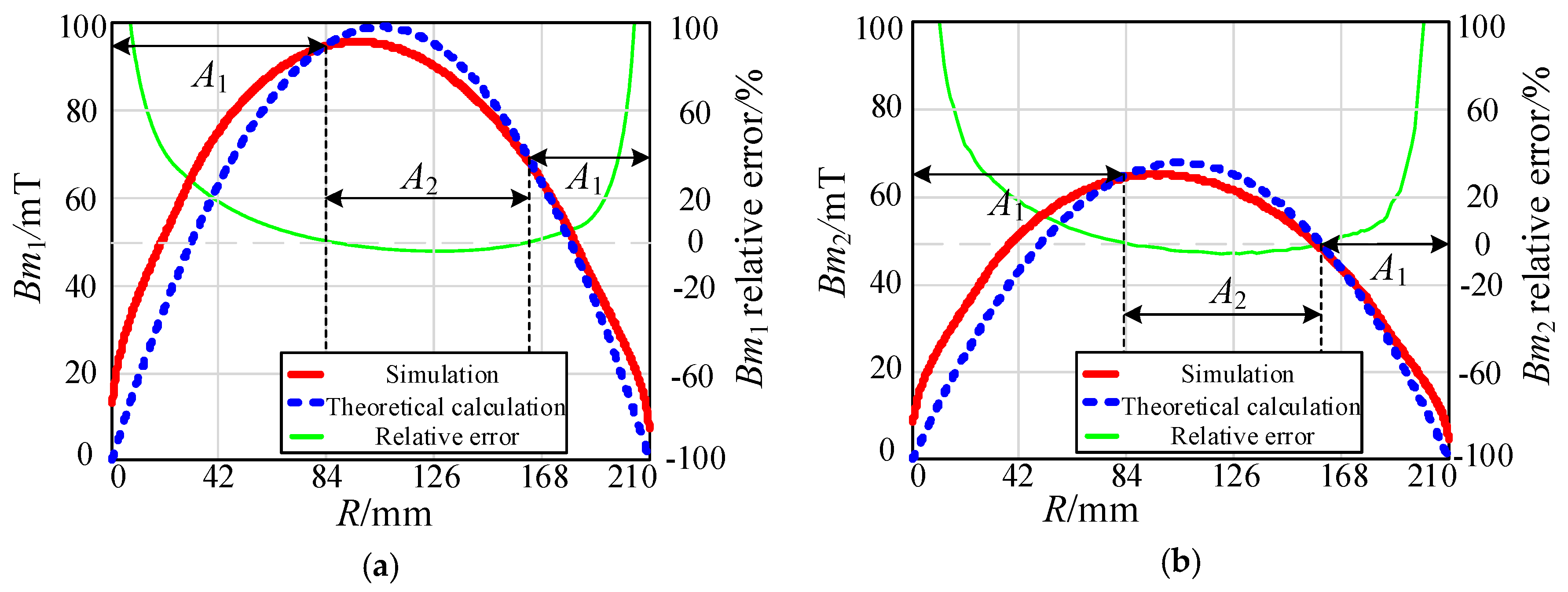
The magnetic flux density distribution inside the transmitter core and the receiver core obtained by theoretical model calculation and FEA simulation are compared, as shown in Figure 7. Where the transmitter winding current I_p = 12 A, the receiver winding current I_s = 18 A and phase-shift = 0°.

The tendency of the magnetic flux density obtained from the theoretical model and the simulation is basically consistent, but some areas are different. The magnetic flux density calculated by the theoretical model is larger than the magnetic flux density of simulation in the A₂ area, and smaller than the magnetic flux density of simulation in the A₁ area. The core loss is mainly determined by the A₂ area, where the magnetic flux density is relatively large. The maximum absolute value of the relative error of the magnetic flux density Bm₁ in the A₂ area is 2.57%; the relative error of the core loss determined by the relative error of the Bm₁ is 5.97%.

For the calculation of the core loss, the theoretical calculation result of the core loss is slightly larger than the simulation result in the A₂ area, while it is opposite in the A₁ area. On the whole, the relative error of the overall core loss becomes smaller.

3.3. Core Loss Modeling

The calculation method of core loss generally adopts the Steinmetz formula proposed by C.P. Steinmetz [31]; the expression is:

$$P_{\mathrm{core}}=k·f^{\alpha }·B_m{}^{\beta }·V_{\mathrm{e}}$$

(21)

where P_core is the core loss of magnetic component; f is frequency; V_e is the volume of the magnetic component; k, α, and β are the empirical parameters obtained from the experimental measurement. Formula (21) is suitable for applications where the core loss is at a certain frequency and magnetic flux density of the magnetic component.

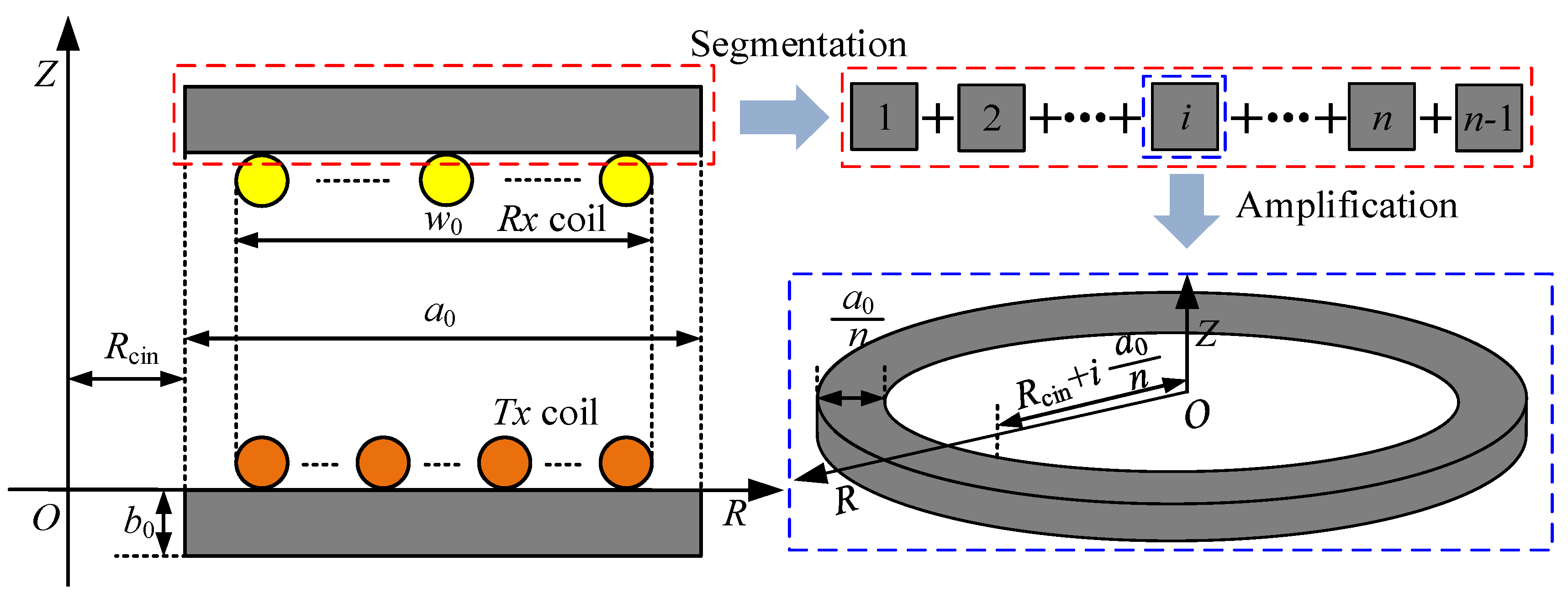
Since the magnetic flux density of the disk core across each circle sheet of core is different, the core loss cannot be calculated directly by the Steinmetz formula. The concept of this paper is as follows: Firstly, the disk core is divided into several circle sheets along the radial direction; then, the core loss of each circle sheet is calculated through the Steinmetz formula; and finally, the whole disk core loss is calculated by the summation of all circle sheets.

While the distance between the inner radius and the outer radius of the magnetic core is a₀; the distance between the inner radius and the outer radius of the winding is w₀. The magnetic core is equally divided into n circle sheets along the radial direction as shown in Figure 8.

It can be seen from Figure 8 that the volume of the i-th magnetic core can be expressed as:

$$V_{\mathrm{core}}(i)=2\mathsf{\pi }\frac{a_0}{n}(\frac{a_0}{n}i+R_{\mathrm{cin}})b_0$$

(22)

The magnetic flux density distribution of the magnetic core along the radial direction is Bm(R), when n is large enough; the magnetic flux density in a circle sheet can be approximately regarded as constant. Then, according to the Steinmetz formula, the core loss of the i-th circle sheet core can be expressed as:

$$P_{\mathrm{core}\_\mathrm{unit}}(i)=k{f}^{\alpha }{\left[B_m(\frac{a_0}{n}i)\right]}^{\beta }2\mathsf{\pi }\frac{a_0}{n}(\frac{a_0}{n}i+R_{\mathrm{cin}})b_0$$

(23)

The core losses of the n circle sheet cores are summed, and then the core loss of the whole disk core can be expressed as:

$$P_{\mathrm{core}}={\displaystyle \sum _{i=1}^{n}k{f}^{\alpha }{\left[B_m(\frac{a_0}{n}i)\right]}^{\beta }2\mathsf{\pi }\frac{a_0}{n}(\frac{a_0}{n}i+R_{\mathrm{cin}})b_0}$$

(24)

Formula (25) can be obtained by combining Formulas (17), (20) and (24); the core losses of the transmitter core and the receiver core can be expressed as:

$$\{\begin{array}{l}{P}_{1\mathrm{core}}={\displaystyle \sum _{i=1}^{n}k{f}^{\alpha }{\left[\frac{-4B{m}_{1\max }}{a_0{}^2}{(\frac{a_0}{n}i)}^2+\frac{4B{m}_{1\max }}{a_0}(\frac{a_0}{n}i)\right]}^{\beta }2\mathsf{\pi }\frac{a_0}{n}(\frac{a_0}{n}i+R_{\mathrm{cin}})b_0}\\ P_{2\mathrm{core}}={\displaystyle \sum _{i=1}^{n}k{f}^{\alpha }{\left[\frac{-4B{m}_{2\max }}{a_0{}^2}{(\frac{a_0}{n}i)}^2+\frac{4B{m}_{2\max }}{a_0}(\frac{a_0}{n}i)\right]}^{\beta }2\mathsf{\pi }\frac{a_0}{n}(\frac{a_0}{n}i+R_{\mathrm{cin}})b_0}\end{array}$$

(25)

4. Simulation and Verification

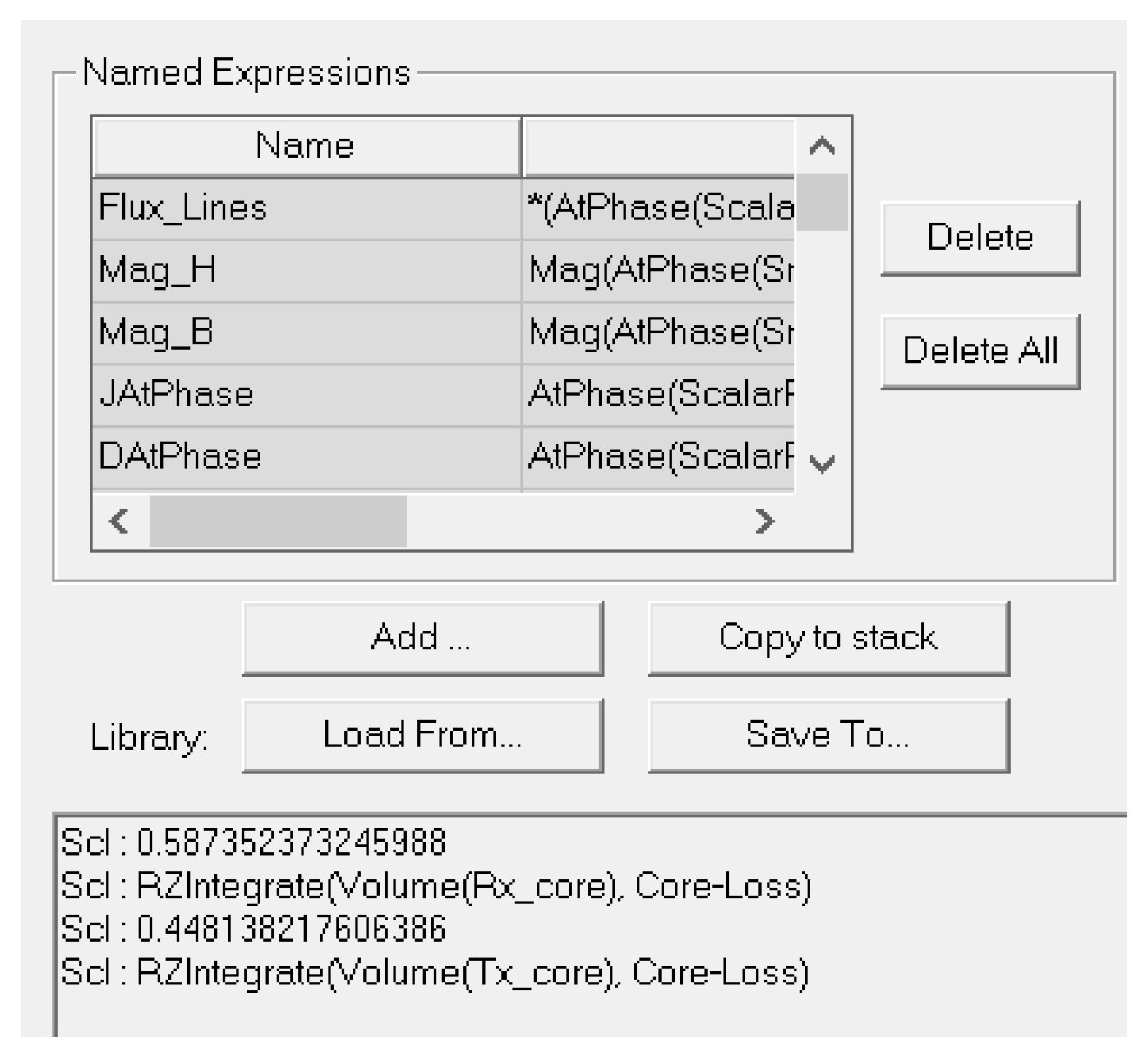
It is assumed that I_p = 4 A, I_s = 8 A, phase-shift = 35°. The core loss at a given operating point is obtained under FEA simulation, as shown in Figure 9. In the same way, the core loss under different coil currents and different current phase-shift can also be obtained by FEA simulation. The core losses obtained by the theoretical model and FEA simulation are compared at different operating points, and then the results are drawn in the same figure by Mathcad15 software.

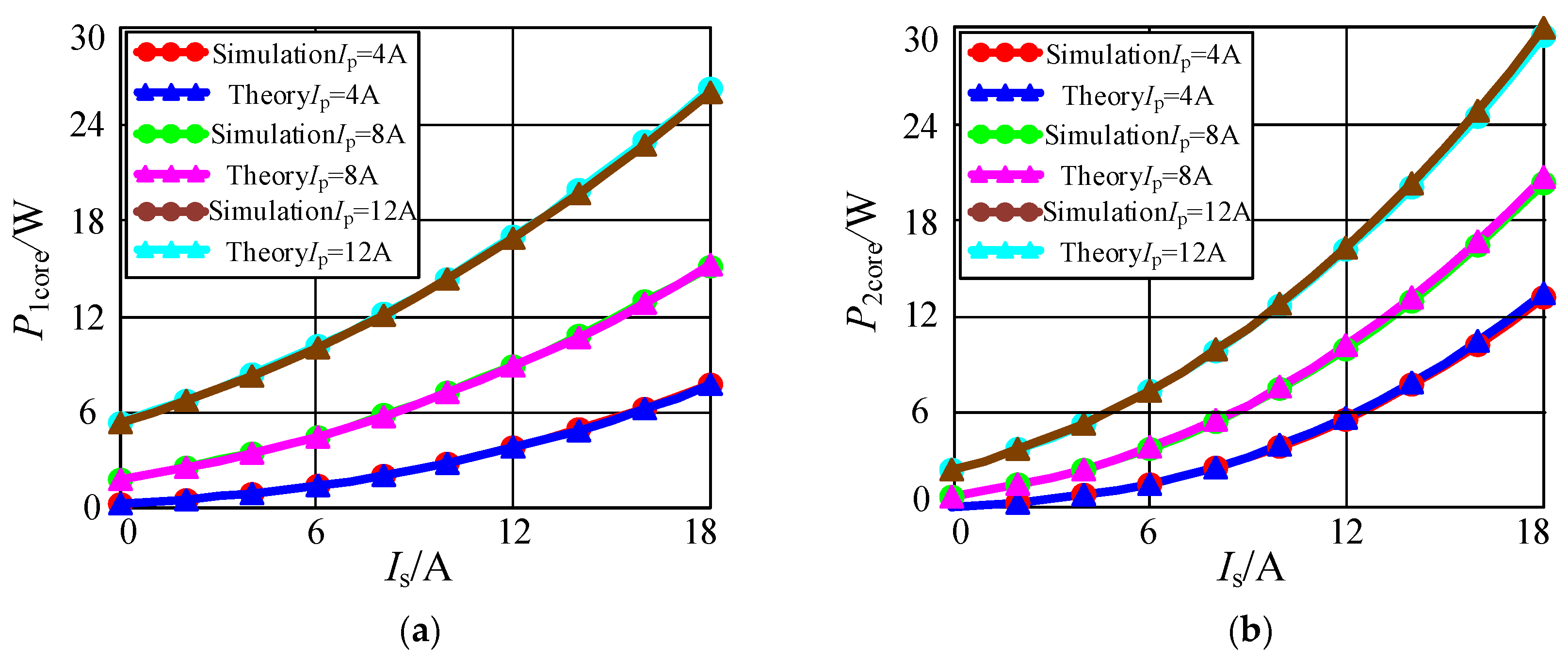
The core losses of the transmitter core and the receiver core obtained by theoretical model calculation and FEA simulation are compared under different winding currents, as shown in Figure 10, where there is no phase-shift between the transmitter winding current and the receiver winding current.

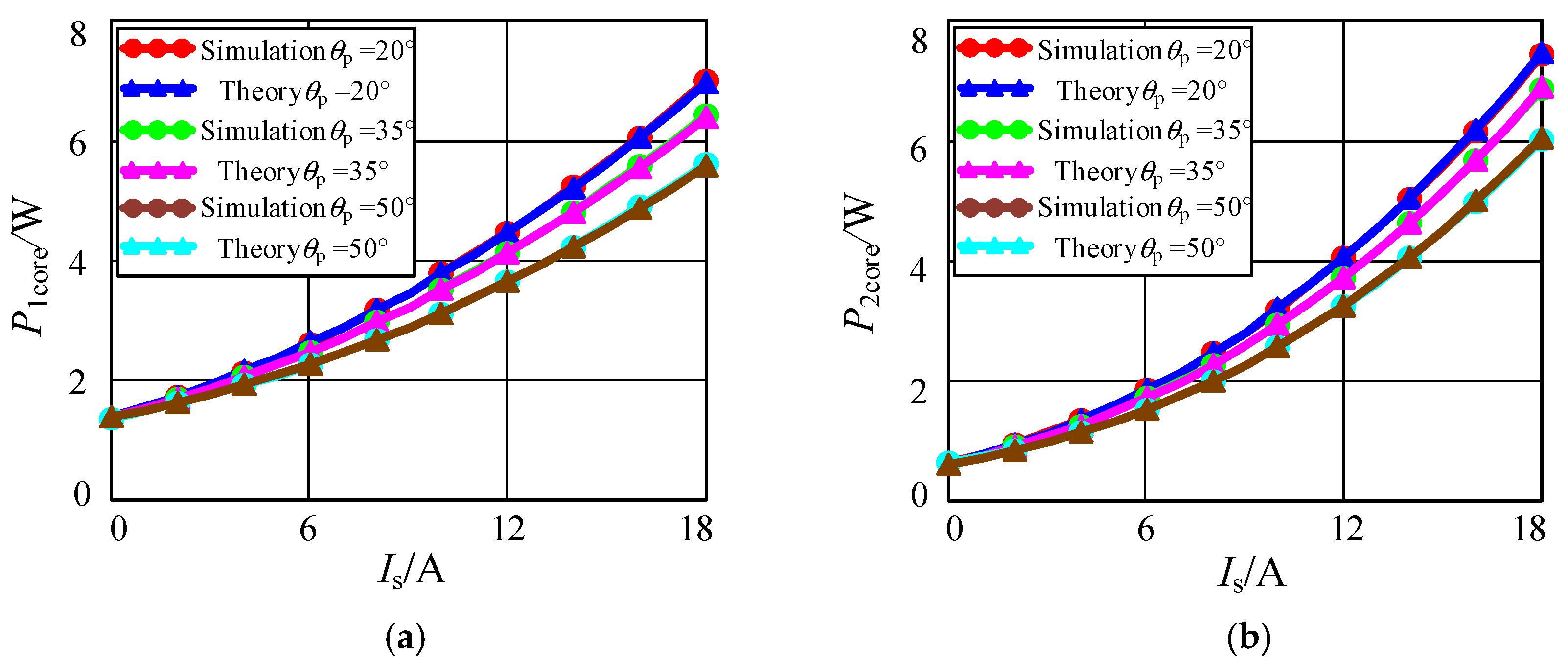
In the same way, the core losses of the transmitter core and the receiver core obtained by theoretical model calculation and FEA simulation are compared under different phase-shifts, as shown in Figure 11, where the transmitter winding current I_p = 12 A.

The core losses obtained by the theoretical model and FEA simulation are basically consistent at different operating points, as the core loss is mainly determined by the area where the magnetic flux density is relatively large. In areas where the relative error of the magnetic flux density is relatively small, the relative error of the core loss determined by the magnetic flux density is also relatively small. Hence, the FEA simulation results show that the magnetic core loss calculated by the proposed model has good accuracy.

5. Conclusions

The article studies and analyzes the magnetic flux density inside the disk core and establishes the corresponding core loss model. The conclusions are as follows:

• The magnetic flux density inside the disk core through each radial circle sheet core is different; consequently, the average magnetic flux density cannot be used to calculate the overall core loss because of the non-linear core loss characteristic of the magnetic core.
• In the core loss calculation, the distribution of the magnetic flux density in the core needs to be taken into consideration. According to FEA simulation results, the mathematical model of the distribution of magnetic flux density is established. This model can be described as a quadratic function in which the parameters are extracted from the magnetic-field distribution of the magnetic coupling system.
• In order to build the disk core loss model of the WPT system, the disk core is divided into several circle sheets. In each circle sheet, the magnetic flux density can be seen to be the same and the core loss can be calculated by the Steinmetz formula. Combining the model of the distribution of magnetic flux density inside the magnetic core, the disk core loss model of the WPT system is proposed.
• The FEA simulation results show that the magnetic core loss calculated by the proposed model has good accuracy. This core loss model can provide an easier way to calculate the disk core loss of the WPT system than the FEA simulation.

References

- Chan, C.C.; Bouscayrol, A.; Chen, K. Electric, Hybrid, and Fuel-Cell Vehicles: Architectures and Modeling. IEEE Trans. Veh. Technol. 2010, 59, 589–598. [Google Scholar] [CrossRef]
- Griffith, P.; Bailey, J.R.; Simpson, D. Inductive Charging of Ultracapacitor Electric Bus. World Electr. Veh. J. 2008, 2, 29–37. [Google Scholar] [CrossRef]
- Zhao, Z.M.; Zhang, Y.M.; Chen, K.N. New Progress of Magnetically-Coupled Resonant Wireless Power Transfer Technology. Proc. Chin. Soc. Electr. Eng. 2013, 33, 1–13. [Google Scholar]
- Costanzo, A.; Dionigi, M.; Masotti, D.; Mongiardo, M.; Monti, G.; Tarricone, L. Electromagnetic Energy Harvesting and Wireless Power Transmission: A Unified Approach. Proc. IEEE 2014, 102, 1692–1711. [Google Scholar] [CrossRef]
- Papastergiou, K.D.; Macpherson, D.E. An airborne radar power supply with contactless transfer of energy—Part I: Rotating transformer. IEEE Trans. Ind. Electron. 2007, 54, 2874–2884. [Google Scholar] [CrossRef]
- Liu, X.; Hui, S.Y. Simulation study and experimental verification of a universal contactless battery charging platform with localized charging features. IEEE Trans. Power Electron. 2007, 22, 2202–2210. [Google Scholar]
- Kim, H.J.; Hirayama, H.; Kim, S.; Han, K.J.; Choi, J.W. Review of Near-Field Wireless Power and Communication for Biomedical Applications. IEEE Access 2017, 5, 21264–21285. [Google Scholar] [CrossRef]
- Meyers, D.; Willis, K. Sorting Through the Many Total-Energy-Cycle Pathways Possible with Early Plug-In Hybrids. World Electr. Veh. J. 2008, 2, 66–88. [Google Scholar] [CrossRef] [Green Version]
- Zhao, Z.; Liu, F.; Chen, K. New Progress of Wireless Charging Technology for Electric Vehicles. Trans. China Electro.-Tech. Soc. 2016, 31, 30–40. [Google Scholar]
- Choi, S.Y.; Jeong, S.Y.; Gu, B.W.; Lim, G.C.; Rim, C.T. Ultraslim S-Type Power Supply Rails for Roadway-Powered Electric Vehicles Generalized Models onSelf-Decoupled Dual Pick-Up Coils for a Large Lateral Tolerance. IEEE Trans. Power Electron. 2015, 30, 6456–6468. [Google Scholar] [CrossRef]
- Wang, Z.Y.; Wang, X.M.; Zhang, B.; Qiu, D.Y. Advances of Wireless Charging Technology in Electric Vehicle. J. Power Supply 2014, 3, 27–32. [Google Scholar]
- Meyers, D.; Willis, K. Globally Cool Vehicles: When Only Electric Will Do. World Electr. Veh. J. 2008, 2, 10–18. [Google Scholar] [CrossRef]
- Asfani, D.A. Electric Vehicle Research in Indonesia: A Road map, Road tests, and Research Challenges. IEEE Electrif. Mag. 2020, 8, 44–51. [Google Scholar] [CrossRef]
- Zhang, W.J.; Bi, L.F.; Ming, L.Y.; Song, J.C.; Jia, L.; Ren, H. Research on Misalignment Performance of Magnetic Coupling Structure in Magnetically Coupled Resonant Wireless Power Transfer System. High. Volt. Eng. 2020, 46, 4087–4095. [Google Scholar]
- Kavitha, M.; Bobba, P.B.; Prasad, D. A Study on Effect of Coil Structures and Core Configurations on Parameters of Wireless EV Charging System. In Proceedings of the 2017 IEEE Transportation Electrification Conference (ITEC), Pune, India, 13–15 December 2017; pp. 1–6. [Google Scholar]
- Xiao, C.; Chen, G.; Odendaal, W.G.H. Overview of Power Loss Measurement Techniques in Power Electronics Systems. IEEE Trans. Ind. Appl. 2007, 43, 657–664. [Google Scholar] [CrossRef]
- Tan, F.D.; Vollin, J.L. A Practical Approach for Magnetic Core-Loss Characterization. IEEE Trans. Power Electron. 1995, 33, 124–130. [Google Scholar]
- Hou, D.; Mu, M.; Lee, F.C.; Li, Q. New High-Frequency Core Loss Measurement Method with Partial Cancellation Concept. IEEE Trans. Power Electron. 2017, 32, 2987–2994. [Google Scholar] [CrossRef]
- Thottuvelil, V.J.; Wilson, T.G. High-frequency measurement techniques for magnetic cores. IEEE Trans. Power Electron. 1990, 5, 41–53. [Google Scholar] [CrossRef]
- Han, Y.; Liu, Y.F. A Practical Transformer Core Loss Measurement Scheme for High-Frequency Power Converter. IEEE Trans. Ind. Electron. 2008, 55, 941–948. [Google Scholar] [CrossRef]
- Dai, X.; Li, X.; Li, Y.; Hu, A.P. Maximum Efficiency Tracking for Wireless Power Transfer Systems with Dynamic Coupling Coefficient Estimation. IEEE Trans. Power Electron. 2018, 33, 5005–5015. [Google Scholar] [CrossRef]
- Yao, Y.; Wang, Y.; Liu, X.; Lu, K.; Xu, D. Analysis and Design of an S/SP Compensated IPT System to Minimize Output Voltage Fluctuation Versus Coupling Coefficient and Load Variation. IEEE Trans. Veh. Technol. 2018, 67, 9262–9272. [Google Scholar] [CrossRef]
- Iero, D.; Corte, F.; Fiorentino, G. A Calorimetry-Based Measurement Apparatus for Switching Losses in High Power Electronic Devices. In Proceedings of the 2016 IEEE International Energy Conference (ENERGYCON), Leuven, Belgium, 4–8 April 2016; pp. 1–5. [Google Scholar]
- Szabados, B.; Mihalcea, A. Design and Implementation of a Calorimetric Measurement Facility for Determining Losses in Electrical Machines. IEEE Trans. Instrum. Meas. 2002, 51, 902–907. [Google Scholar] [CrossRef]
- Sun, C.; Shi, Z.; Shi, L.; Yue, C.; Yu, J. Measurement of LVDC Customer-end Inverter Efficiency by Calorimetry Method. In Proceedings of the 2019 IEEE Sustainable Power and Energy Conference (iSPEC), Beijing, China, 21–23 November 2019; pp. 2708–2712. [Google Scholar]
- Chen, B.; Li, L.; Zhao, Z. Magnetic Core Losses Under High-Frequency Typical Non-Sinusoidal Voltage Magnetization. Trans. China Electrotech. Soc. 2018, 33, 1696–1704. [Google Scholar]
- Yu, X.; Li, Y.; Yang, Q.; Yue, S.; Zhang, C. Loss Characteristics and Model Verification of Soft Magnetic Composites Under Non-Sinusoidal Excitation. IEEE Trans. Magn. 2019, 55, 1–4. [Google Scholar] [CrossRef]
- Jung, Y.W.; Kim, H.K. Prediction of Nonlinear Stiffness of Automotive Bushings by Artificial Neural Network Models Trained by Data from Finite Element Analysis. Int. J. Automot. Technol. 2020, 21, 1539–1551. [Google Scholar] [CrossRef]
- Zhang, W.; Chen, Q.; Wong, S.C.; Tse, M.; Cao, L. Reluctance Circuit and Optimization of a Novel Contactless Transformer. Proc. Chin. Soc. Electr. Eng. 2010, 30, 108–116. [Google Scholar]
- Lee, W.Y. Finite-Width Magnetic Mirror Models of Mono and Dual Coils for Wireless Electric Vehicles. IEEE Trans. Power Electron. 2013, 28, 1413–1428. [Google Scholar] [CrossRef]
- Steinmetz, C.P. On the Law of Hysteresis. Trans. Am. Inst. Electr. Eng. 1892, 9, 1–64. [Google Scholar] [CrossRef]
Figure 1.
The simulation model of the magnetic coupling system.
Figure 2.
The distribution of magnetic flux density inside the transmitter core and the receiver core.
Figure 3.
The distribution of magnetic flux density inside the transmitter core. (a) The distribution of magnetic flux density versus R-axis; (b) The distribution of magnetic flux density versus Z-axis.
Figure 4.
The simplified magnetic flux density distribution inside the disk core.
Figure 5.
The schematic diagram of the magnetic field line distribution in the magnetic coupling system.
Figure 6.
The method of images equivalent model. (a) The magnetic coupling system model; (b) The method of images model of transmitter winding current; (c) The method of images model of receiver winding current.