1. Introduction
Climate change caused by greenhouse gases is generally seen as a key challenge humanity is facing in the 21st century. The mobility sector is one of the main drivers of emissions and must become carbon neutral shortly to avoid catastrophic consequences. For personal mobility, electric vehicles (EVs) are currently favored by many practitioners and academics as a technology for decarbonisation. The ongoing increase of EVs must be accompanied by an increase in available public charging infrastructure (CI). The CI can be divided into two groups, the fast-charging mostly DC network and the slow-charging AC network. The former is necessary to enable long-distance highway traveling generally and drivers stay near the vehicle during the short charging periods. The latter is the key enabler for everyday mobility and can be further differentiated into private and public charging. Private charging takes place at households or workplaces. Public charging occurs at openly accessible charging stations (CS) in parking areas, while the EV drivers are usually engaged in other activities such as shopping, sports, etc. Due to the generally longer charging times, it is important to place the CSs at attractive locations, so that the users can integrate the charging process into their daily life. Further, to make the CSs worthwhile for the operators, a high frequency of usage is important. Failing to do so could mean that the expensive and often publicly supported CSs may remain unused. These ideas motivate this paper’s goal of supporting the process of selecting suitable locations.
A large and growing body of literature has investigated and debated the topic of site selection for charging infrastructure. In the absence of sufficient usage data or for projections into the future, the models are typically based on socio-demographic data including points of interest (POI) [
1], expert interviews [
2,
3], traffic counters [
4,
5], and user surveys [
6,
7]. However, the lack of real-world utilization data reference in these approaches implies the use of fundamental assumptions. Users could state preferences and behavior that does not coincide with the actual reality. Expert opinions and socio-demographic data have no direct link to actual usage meaning that the people’s behavior can only be approximated. Realized CSs usage may therefore significantly differ from the anticipations made.
An alternative approach to the above-stated methods is to analyze data of CS or EV usage [
8,
9,
10,
11,
12,
13,
14]. The most frequently used method in these works is to use ordinary least squares linear regression to find correlations between CS usage and external features. For the placement of new infrastructure, dynamic features are of little relevance since the location of a CS does not change. Dynamic approaches are useful in peak demand and load management. The list of analyzed features can be categorized along the properties of time-varying and static one axis and geographical scope on the other axis. Examples of time-varying external features are, for example, the time of day, as is common for electrical load profiles. In a larger scope, regional effects such as school vacations, public holidays, or weather can cause time-varying behavior. Local specific features that influence the charging behavior can be for example traffic hot spots or local events. For static features, area-based and point-based features are the most suitable, such as population density or the type of POIs nearby. Using this classification, researchers typically create a linear regression model that links the CS usage and the available external features [
14,
15]. The approach of using
POI data or other types of Geographic Information System (GIS) data is not new and has been used by other researchers as well. The authors in [
15] find potential CS locations by requiring that features such as public transportation, major road access, population centers, stores, industrial centers, etc., are all nearby. However, this static approach is based entirely on GIS data from external features. Information on the utilization of existing charging stations to validate their assumptions was not taken into account. The authors in [
14] had access to both CS occupation and GIS data, in particular POIs, and their work can therefore be considered as an evolution from [
15]. They mapped CS usage to nearby POIs and were thereby able to create a map of attractiveness for the area under investigation. The limitation, however, is that the geographic areas analyzed are comparatively small and therefore limited in scope. This makes it challenging to verify the applicability of the encountered trends to a broader geographic area.
As was shown in the previous paragraph, there is a great deal of attention in the literature on methods of selecting suitable locations for the expansion of CI. However, the applicability of proposed methodologies to a larger scale remains questionable due to the limited data in previous studies, especially for methods combining CS usage and POIs. This limitation on local data makes the results more prone to spurious correlations and overestimation of local phenomena. For greater applicability, the research question hence needs to be examined with a much greater and more diverse geographic scope. Another issue is that since researchers in the past were unable to test their findings on a national scale, it was challenging to extrapolate how new charging infrastructure would be created. Therefore, we focus on static properties, specifically on area and location data, as well as real-world CS occupation data. By using a large data basis encompassing CS usage and POI locations up to a national scope, this paper aims to contribute to the charging station site selection in Germany. The sheer size of the data set enables robust statistical statements about the correlation between CS usage and POIs. Consequently, the results are less susceptible to local effects that cannot be reflected in the POI data.
To do so, we use regression analysis to identify the impact of specific POI categories on the charging station utilization. Using the regression fit function, we create heat maps indicating the charging station site attractiveness. We use these heat maps to find new sites for CSs that maximize their attractiveness by performing a genetic optimization with two different strategies. The first strategy is called “competing” and aims to maximize the attractiveness of every new build CS. The second strategy is called “cooperating” and aims to maximize the overall attractiveness of the area under consideration by placing new CSs. The results are presented and discussed afterward, followed by a discussion about the limitations of our work. Last, the results are concluded, pointing out several key findings.
2. Data
2.1. Charging Station Utilization
The data used for the analysis are the charging station availability that is accessible via different platforms in Germany [
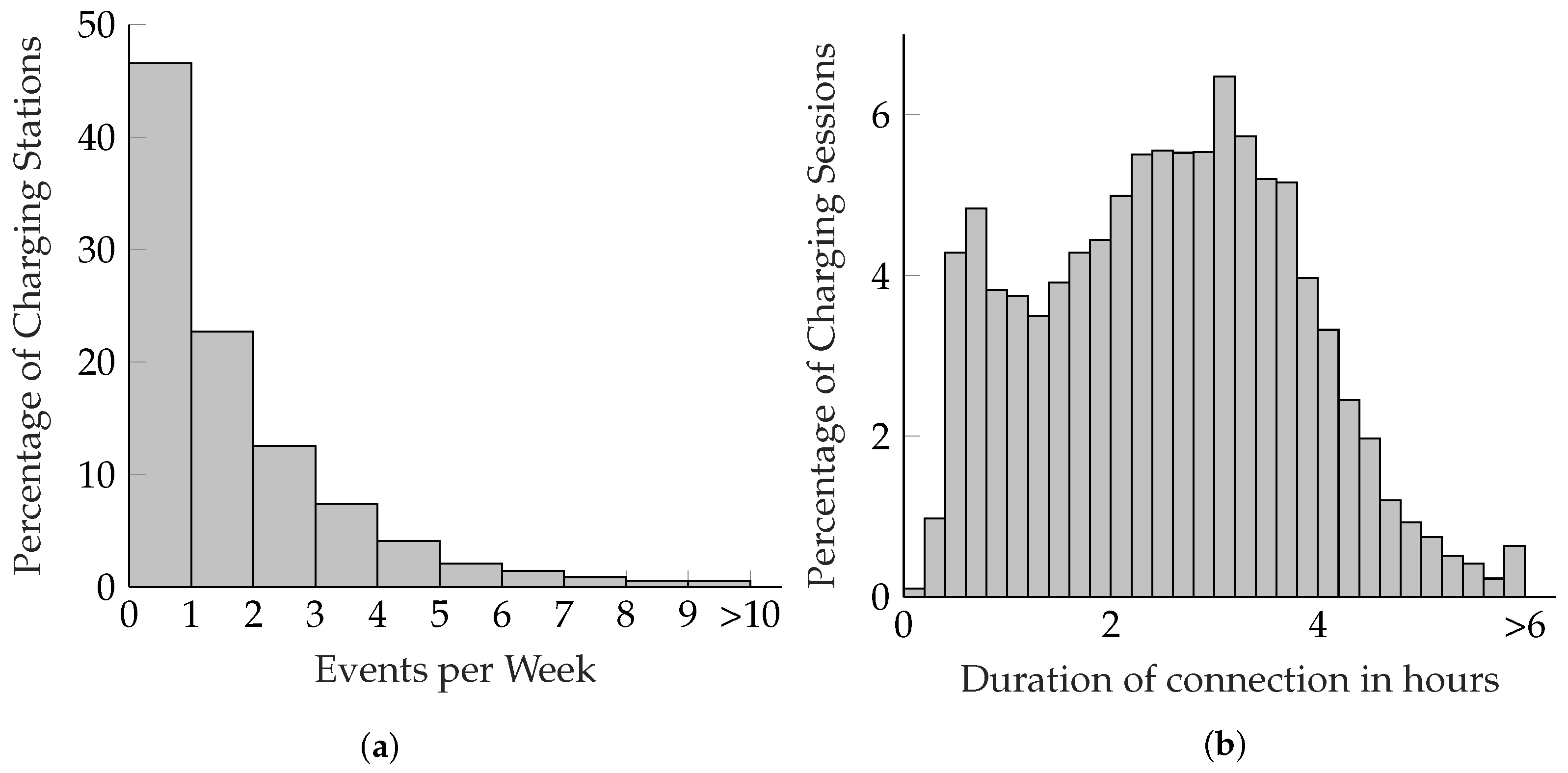
8]. Our data set consists of 21,777 charging points (CPs) in urban and suburban areas in Germany. It includes mostly AC charging points and a few DC fast-charging points. Large fast-charging networks along highways, comparable to service stations, are not included in the data set. For approximately one year, 1,836,076 charging events have been recorded. According to the terminology used in this paper, a charging event is defined as the period in which an EV occupies a CP, as our data do not contain any information about the exact charging process. For each CP, we calculate the key performance indicators (KPIs) charging events per week and average event duration. Furthermore, the overall recording time for each charging point is determined. This parameter may vary as more data sources were gradually added over time to the data set, and some CSs did not provide continuous data for all CPs. On average, the recorded data per
CP is 311 days, which corresponds to a representative period, as also seasonal charging behavior is included. The data reveals that most CPs are used less than once per week, while the average utilization amounts to 1.8 charging events per week (see
Figure 1a). The histogram in
Figure 1b) on average durations of charging events reveals a significant spread across the analyzed CPs, with an average duration of 2:34 h. There are two maxima at charging durations around 30 min and 3 h, respectively. As the low average utilization already indicates, there are significant regional differences in the economic efficiency of charging stations. A detailed analysis based on the same data can be found in [
16]. For the economic operation of an AC charging point, at least one charging process of about four hours per day is necessary.
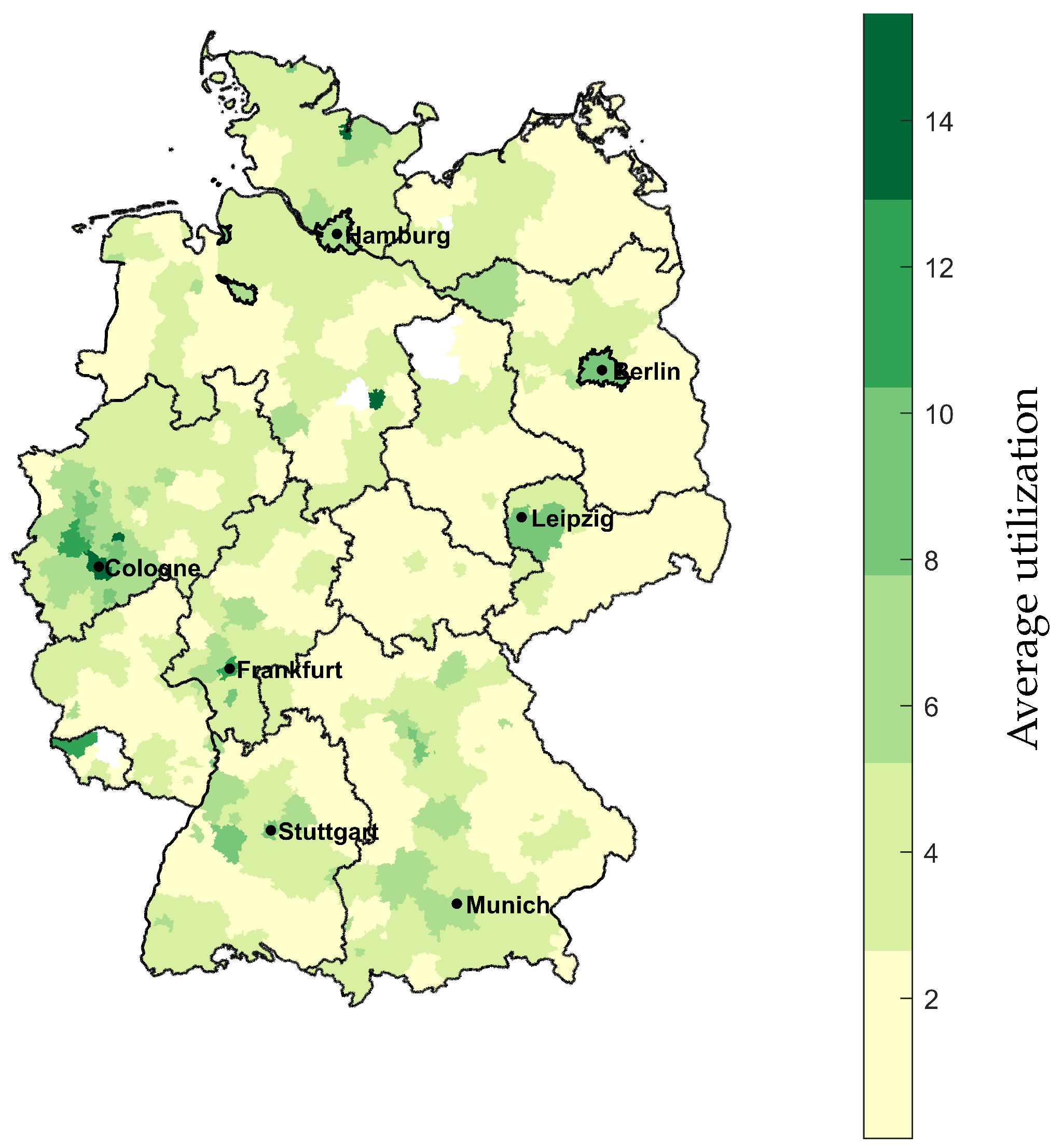
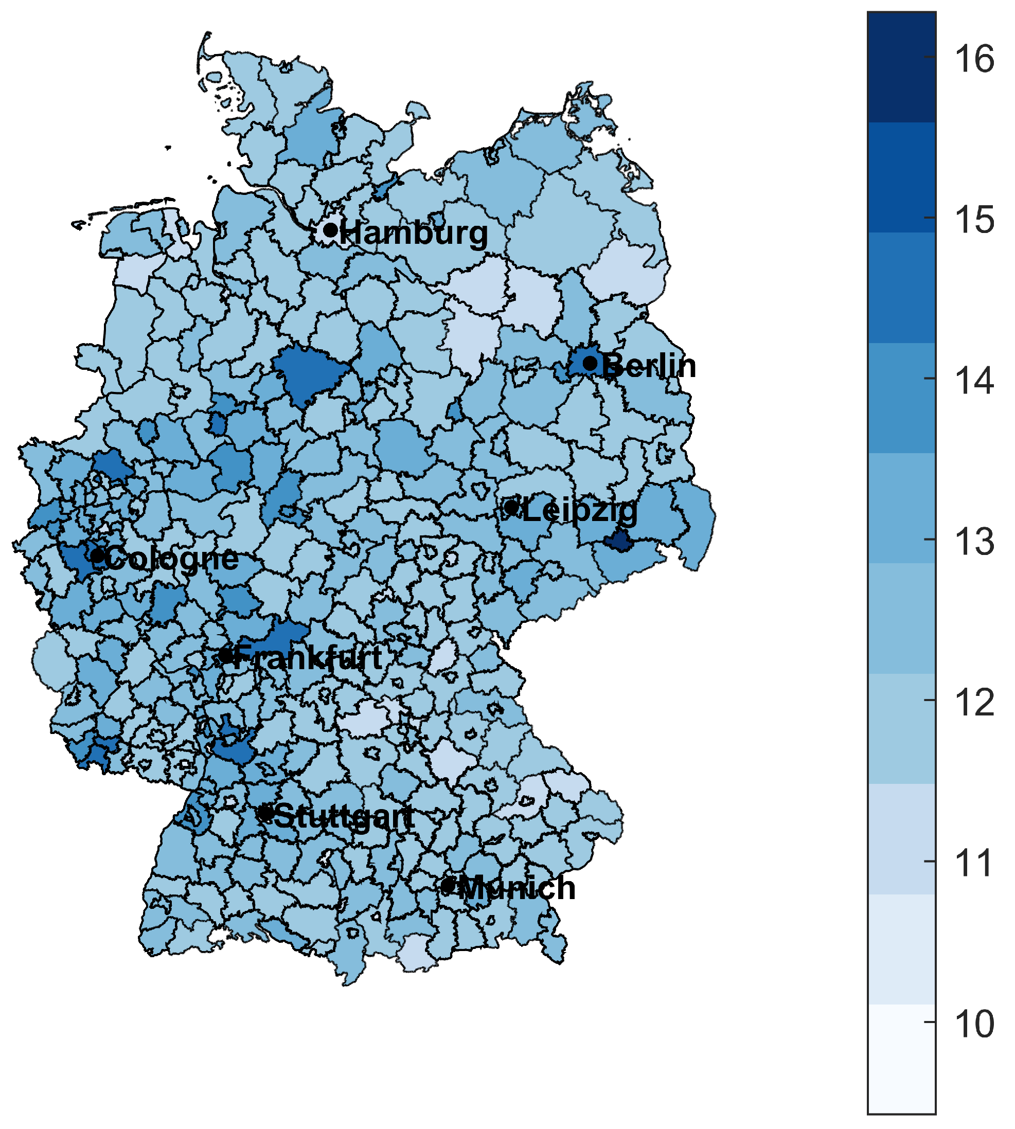
For spatial analysis, the data are grouped based on the 401 administrative districts of the German counties and independent cities. The 21,777 CPs in our data cover 375 of these districts. To evaluate the performance of a
CP in terms of empirical user acceptance and utilization, a metric proposed in [
17] is applied, which is defined as the product of average charging events per week and average charging duration per event. This KPI is calculated for every charging station and averaged for the regions. The large spread in
CP performance between individual German districts is depicted in
Figure 2.
2.2. Points of Interest
A
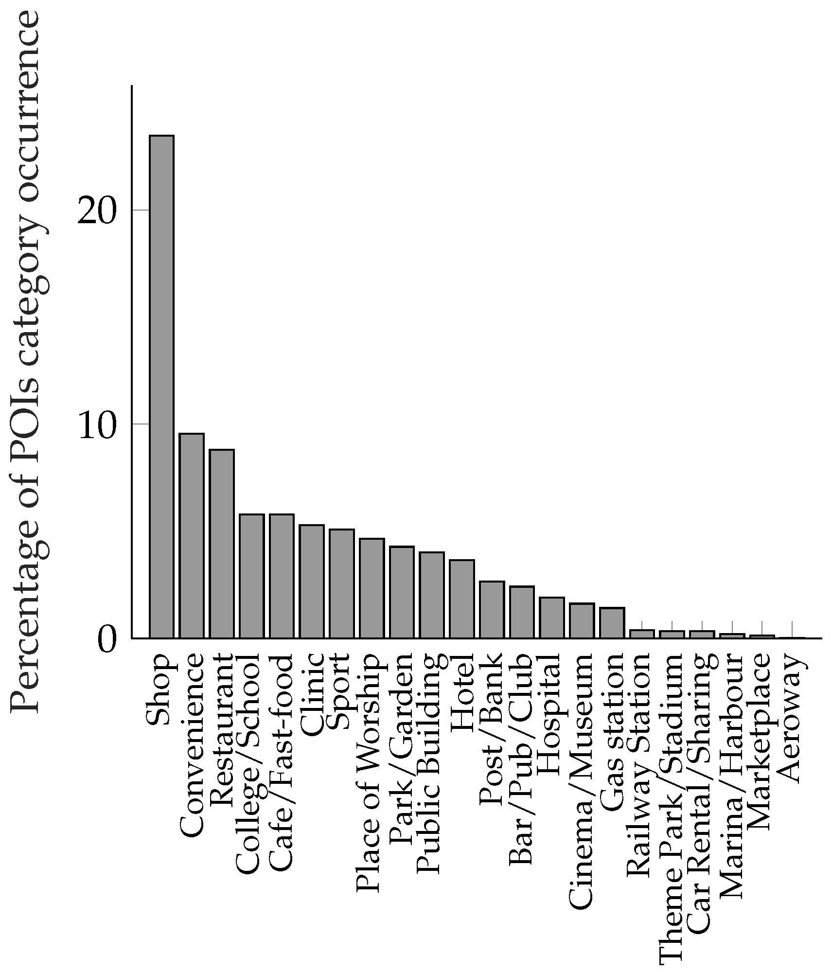
POI is a location of particular interest for public life, such as schools, restaurants and shopping locations. Thus, it represents a frequently visited destination for pedestrians, cyclists and, car owners alike. We use POIs located and characterized in the OpenStreetMap (OSM) service. These POIs can be used to characterize areas based on the category and frequency of occurrence. For example, an area with a high number of restaurants and bars could be a nightlife district, which is a place of common interest. In residential areas, on the other hand, there are hardly any POIs. In our analysis, we use 23 different
POI categories as shown in
Figure 3 along with their frequency of occurrence. We extract 1,162,387 POIs across Germany, each of which is characterized by its GPS coordinates and category affiliation. The categorization, as well as the frequency of the POIs, are shown in
Figure 3. To extract the OSM POIs, we used the OsmPoisPbf project [
18]. The information on local
POI distribution can be used to assess the attractiveness of a given area for the expansion of charging infrastructure. For this purpose, the methodology used in this paper is presented in the following section.
3. Methodology
3.1. Regression
To identify whether there is a correlation between charging point utilization and the individual
POI categories, we use a linear regression model. As part of the data preparation, the distances of each
CP to the nearest
POI must first be determined for this purpose. We assume that the closer a
POI is placed to a CP, the stronger is its influence on the
CP utilization. Thus, a
POI right next to the
CP has the strongest influence while vanishing with distance. In order to limit the effective area of
POI impact to walking distances, only the POIs within a certain radius
r around the considered
CP location are taken into account in the regression. Assuming a linear characteristic, the effective impact
of the j-th
POI denoted by
on the utilization of the i-th
CP denoted by
is determined by:
where
is a function returning the distance between two points,
N is the total number of charging stations and
K is the number of POIs under consideration. The geographic distances between CPs and POIs are determined using the inverse haversine formula [
19]. POIs with a higher distance than
r= 500 m are assumed to have no influence on the
CP anymore and are set to zero [
14]. A sensitivity analysis of this parameter is carried out in the
Appendix A to further justify our choice of parameter. Subsequently, we perform a multiple linear regression to derive a correlation between the
POI category and the historical utilization of the CPs. In this regression model, the utilization of a given
CP acts as the dependent variable and the corresponding matrix of distances to the nearest POIs
collects the independent variables as described in (
2). Furthermore,
is the vector of the models’ estimates, and
is the error vector.
The predictor values
are calculated using the least-squares regression and are shown in
Table 1 in
Section 4. Based on the linear regression, both positive and negative influences of the
POI category on the utilization can be observed. In addition, we include the population density as a control variable into our model.
3.2. Heat Maps of Attractiveness
Using the fitted regression function, heat maps were generated on the basis of existing POIs and their categories. For this purpose, a dense grid of equidistantly located virtual CPs is created across the considered region. The design matrix
of distances to the nearest POIs is calculated using the virtual CPs. Subsequently, the fitted values
are determined using Equation (
3) and are displayed in the form of a heat map.
Thus, the fitted values can be interpreted as the fraction of the utilization in
Figure 1 that can be explained by the POIs at a specific location. In the following, these values are considered as the attractiveness of a potential location for charging infrastructure. To provide some context for the evaluation of the derived site attractiveness in the heat map, the POIs and the already existing charging stations are also plotted in this figure. In addition to the subsequent analysis of the optimal placement of future CSs, these heat maps can already provide a valuable contribution to rough area planning, as they reduce the area under consideration dramatically to the most promising locations for an adequate charging infrastructure expansion.
3.3. Siting Optimization
Given the previously introduced heat maps, we use this information to find sites for CSs that maximize the attractiveness for users in the following. To achieve this, a three-step method was developed as follows:
- 1.
Creation of a Voronoi graph that allocates areas to the nearest CS,
- 2.
Numerical integration of the attractiveness covered within the intersection area of the walking distance radius and the Voronoi area of a CS,
- 3.
Genetic optimization of the collected attractiveness through additional CS at new sites.
These steps are further described in the following subsections.
3.3.1. Voronoi Graph
A Voronoi graph is a tool that is typically used to partition a given plane with
n points into
n convex polygonal areas such that each of these areas contains only one point. The boundaries between the individual areas are drawn in a way that they are equidistant to the nearest two neighboring points. In this paper, a Voronoi graph is used to define the theoretical coverage areas (polygons) of the given CSs (points) within the region under consideration (plane). For the implementation, the Python package
scipy [
20] was used.
3.3.2. Estimation of Occupation of a Newly Built CS
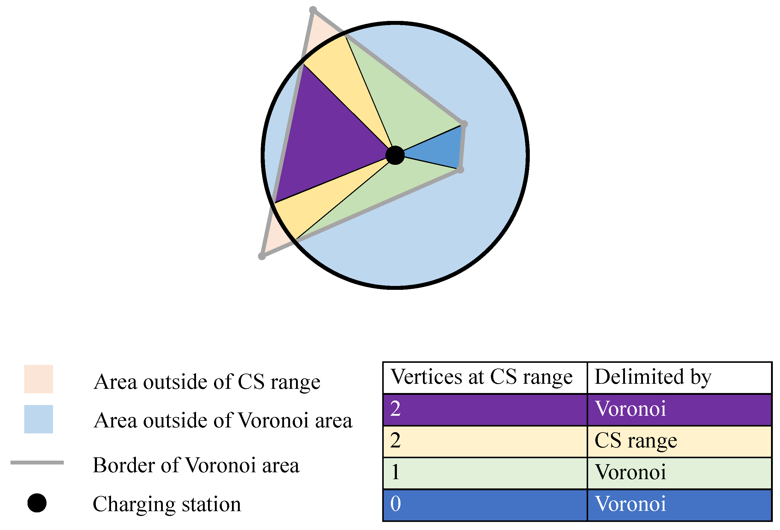
The areas defined by the Voronoi graph are only bounded by the given set of CSs within the borders of the region under consideration. Especially in regions with a low density of CSs, the derived coverage areas may become very large. In practice, the CS defining such a large theoretical coverage area may be the nearest one around. Yet, the most distant locations within the considered area are improbable to be affected by the existence of this CS anymore. Hence, the theoretical coverage area needs to be limited to a practical definition of coverage that is more meaningful for the daily life of EV users. Therefore, a radial boundary with a maximum of 0.01° on the latitude and longitude map (corresponding to approximately 1.1 km) is superimposed on the theoretical coverage area from the Voronoi graph.
Figure 4 illustrates the introduced limitation of the CS coverage area. To simplify the calculation of these covered areas, they are split into several subareas. As
Figure 4, these can be of three different types, which are characterized by how the line opposite to the CS location is delimited and by how many vertices of that line are on the radius defined earlier as the CS range. The purple area is an example of where the Voronoi-boundary is more restrictive than the CS range. The area covered is consequently delimited by the Voronoi boundary and the two radial lines connecting the CS with the two points where Voronoi boundary and CS range meet. The yellow areas are similar, but the range is the limiting factor. The green and blue areas are similar because the Voronoi boundary is more restrictive than the CS range, but either one (green) or two (blue) of the Voronoi vertices are closer to the CS than the CS range. The radial lines are consequently shorter than the CS range. This logic was implemented using Matplotlib [
21] in combination with a pixelated heat map. Once the covered area
is calculated, we determine the captured attractiveness
of a newly built CS using the following loading function
The area of the range limiting circle is used to normalize and hence, can be interpreted as a weighting of how much of the attractiveness that is predicted in the heat map can be actually captured. is the point value of the heat map at the desired location (i.e., the construction site of the CS to be built). Given that the heat map was constructed using the regression results, it can be thought of as an estimation of an occupation rate if no other CSs were nearby. The unit of is identical to the predicted attractiveness of the regression results and can therefore be interpreted as the utilization of a newly built CSs. Since the regression results do not consider competition between the stations, it is important to keep in mind that the utilization will be lower due to the area ratio.
3.3.3. Competing and Cooperating Genetic Optimization
The calculation described in Equation (
4) in the previous section can be interpreted as a target function for optimization with the geographic coordinates of the new CS to be placed serving as optimization inputs. The optimization problem is non-convex and non-monotonous since the heat map does not necessarily have only a single global maximum. Additionally, existing CSs interact with the new CS through the Voronoi borders separating them. An optimization method that is well suited to tackle this kind of problem is genetic optimization. The algorithm works by creating a population of inputs (a list of geographic coordinates) and evaluating their performance. Just like in the real-world evolution, successful members of the population are more likely to create offspring and thereby steadily move the population towards the most promising coordinates. In this work, the python library geneticalgorithm was used [
22]. As inputs to the optimizer, we define two scenarios called “competing” and “cooperating”. In the competing optimization, the target function of the optimizer solely focuses on the attractiveness obtained by the newly built CS. This can be interpreted as a new competitor who aims to position its CS at the most attractive location possible. In the cooperating scenario, the target function is the integral of all CSs in the observed region. This can be interpreted as a monopoly player or a regulatory body trying to maximize coverage of the entire CS network. The key difference is that the algorithm is more willing to place CSs close to each other in the competing scenario than in the cooperating scenario since it is not punished for “stealing” attractiveness from another CS. In the cooperating scenario, this is less attractive since only the additionally covered area contributes to the overall attractiveness.
4. Results
In this section, the results obtained in this paper are presented. We start by providing and evaluating the regression results. These have subsequently been used to generate heat maps which are shown in the next section. For the sake of conciseness, the regression results are exemplified in detail for the city of Cologne, which contains diverse areas ranging from highly urbanized quarters to almost rural suburbs. The two last sections focus on the placement strategies for additional CSs based on the results of the genetic optimization. To compare the different expansion strategies, the resulting placement of the first ten new CSs in the two scenarios is shown. The example of Cologne is used once again to analyze the behavior of the algorithm in detail. This analysis is generalized in a second step by looking at the nationwide results for the cooperating and competing optimization strategies separately. A comparison of the two different optimization strategies concludes this section. All heat maps, the underlying csv-files, and the station placement results can be downloaded from our git repository. The link can be found at the end of this paper.
4.1. Regression
Table 1 shows the results of the regression analysis. As the regression is of a linear nature, both positive and negative influences were expected and obtained. Since all estimates were generated using the same methodology, their values may also be compared. The highly utilized CPs seem to be mostly related to POIs that characterize short-term stays, such as bars, pubs, clubs, schools, colleges, clinics, marketplaces, cinemas, etc., as can be seen from the
POI categories with high estimate values. The high positive correlations for car rental places can possibly be explained by the ca-sharing vehicles also relying on public infrastructure. These interpretations should, however, be taken carefully since there may be hidden factors. One such factor is, for instance, that fast chargers tend to be quite close to gas stations. As [
8] shows, fast chargers have an overall low occupation rate, but given the much shorter charging events, they can service more vehicles than a slow charger. Other POIs such as marinas and harbors, airports, shops, or hotels may be too infrequent so that their predictive value is limited. This is also reflected in the high
p-value, so that the null hypothesis cannot be discarded. Overall, the regression results serve as input for the subsequent steps.
4.2. Heat Maps of Site Attractiveness
An example of the resulting heat map for the city of Cologne can be seen in
Figure 5. It becomes immediately apparent that a high local density of POIs leads to a higher attractiveness of an area. This is not surprising since most estimates in the regression were positive and of larger magnitude than their negative counterparts. A high
POI density corresponds to many amenities and high availability of activities in the surroundings that the EV drivers can turn to while their vehicle is charging. For this reason, the effect of many POIs also leading to high site attractiveness can be well explained and meets expectations.
4.3. Optimization for Charging Infrastructure Expansion
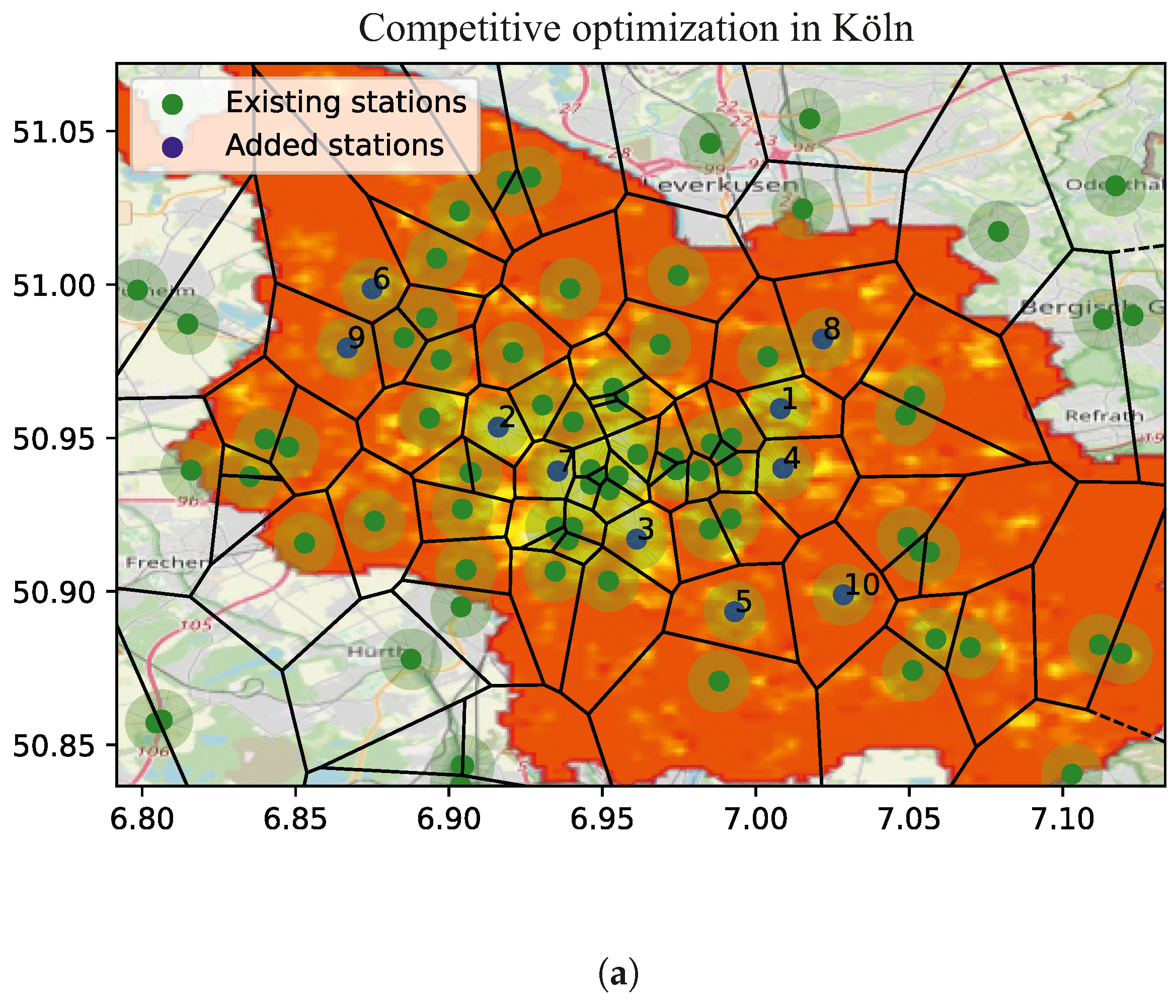
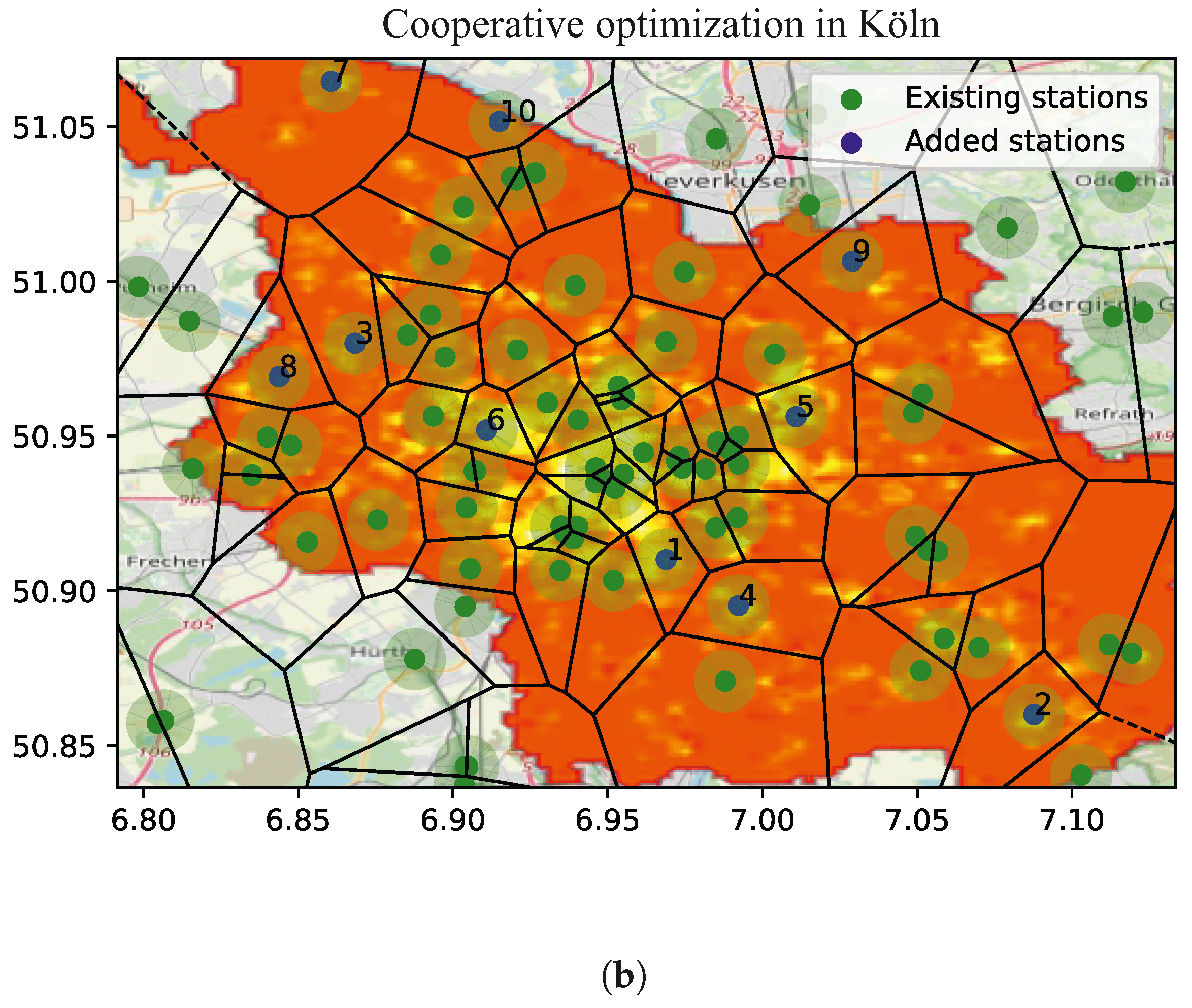
Based on the site attractiveness, the placement of additional CSs has been optimized according to two different expansion strategies, as explained in Section III.C. While the competitive strategy seeks to maximize the captured attractiveness of each CS added, the cooperative strategy focuses on maximizing the coverage area.
Figure 6 shows the optimization results for the example of the city of Cologne where we see a similar behavior for both approaches. The algorithms partially try to fill the gaps in the very attractive areas in the city center (1, 2, 3, 4, 7 for competing and 1, 5, 6 for cooperating). A second option is to pick smaller hotspots further away from the city center (5, 6, 8, 9, 10 for competing and 2, 3, 4, 7, 8, 9, 10 for cooperating). The main difference between the approaches is that the competing strategy results in a lot stronger agglomeration of CSs near the city center and fewer stations in the surrounding area. Further, there are only two stations (5 and 10) in the competing scenario that do not reduce the attractiveness of an existing station. In comparison, the cooperating strategy shows no subtraction of attractiveness for stations 2, 4, 7, and 9 and very limited subtraction for stations 5 and 8. The described behaviors are in line with the optimization goals formulated earlier. We can therefore conclude that the implementation has been successful. Similar checks for other cities confirm the proper operation of the optimization algorithms but are not repeated here for the sake of conciseness. The results are, however, available on our Github repository.
4.4. National Scope
By integrating the attractiveness of the areas covered by CSs in each district, it is possible to gain an understanding of the results on the national level.
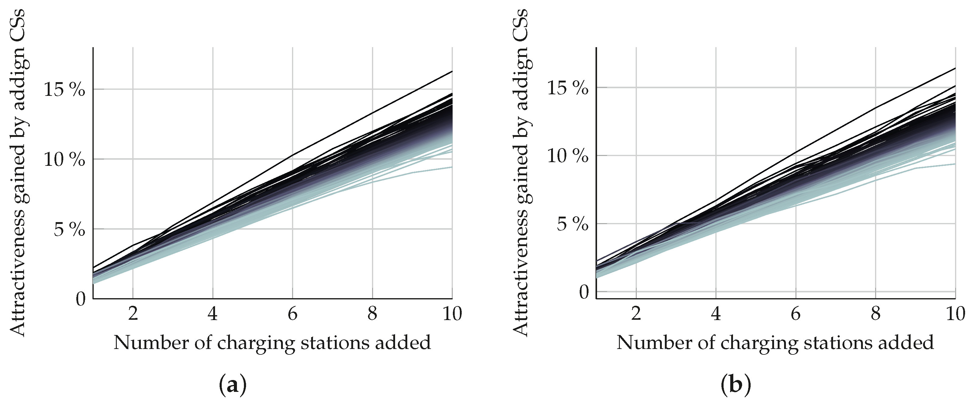
Figure 7 shows the results by looking at the change in achieved attractiveness after CSs are added. When comparing the graphs, it immediately becomes apparent that both approaches perform similarly.
It can be seen that the covered attractiveness across all districts increases with more stations in a linear fashion. This is a strong indication that enough sites are still available for new CSs, and no significant competition has arisen yet. As
Figure 6 shows for the cooperative optimization of Cologne, this is a result of many sites outside the city centers not yet being covered. For the competitive approach, it can be seen that there are sufficient places still available where a new CS can be placed between existing CSs. Both patterns repeat themselves in other locations as well. If only the amount of attractiveness covered is taken as a metric, both strategies perform similarly well and, the average improvement after adding 10 CSs across all districts differs by only 0.6%. This finding can be augmented when including
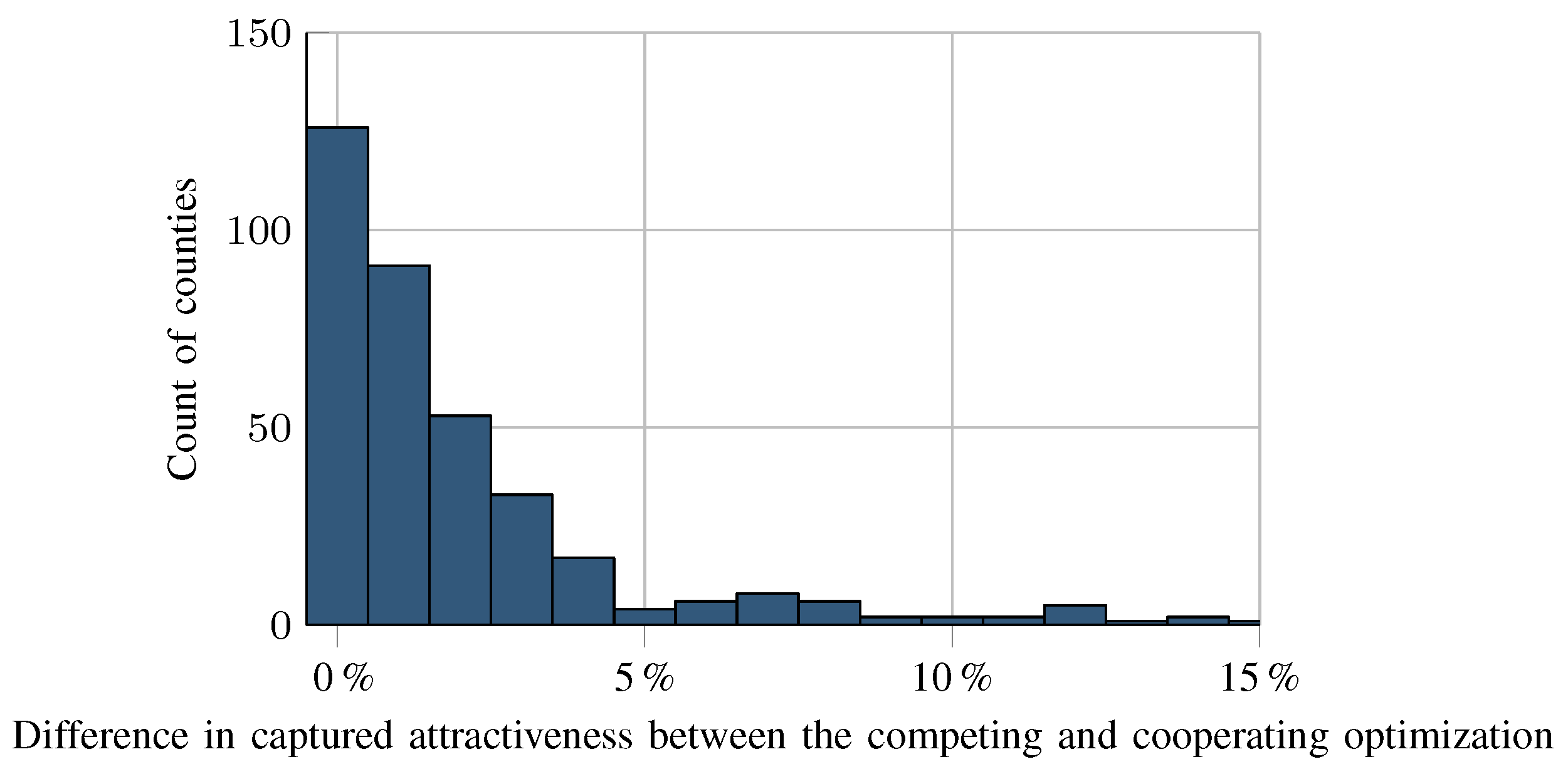
Figure 8. It can be seen that for most counties, the difference between the two approaches results in a captured attractiveness below 5%.
Comparison between Districts
As
Figure 8 shows, the performance difference between competing and cooperating optimization is less than 5% relative to the originally covered attractiveness in 201 out of the 242 districts analyzed. Additionally, districts with a relatively high difference are characterized by having very few CSs at the present time.
In order to provide an understanding of the geographic differences between the individual districts,
Figure 9 projects the gains in captured attractiveness from the optimal placement of ten additional CSs onto a map of Germany. The plot, therefore, shows the values at
x = 10 of the cooperating case in
Figure 7 but is shown on the map to provide a sense of geographical spread. The results illustrate that there is a highly uneven distribution between smaller urban districts and the larger and more rural districts. This effect can also be observed in [
8,
16] where rural areas experience significantly fewer charging events as compared to urban areas. This is not very surprising since population density was included as a factor in the regression model shown in
Table 1 and strongly and positively correlates with attractiveness.
5. Discussion
One key point in the public debate revolving around CSs is how the market should be organized. The currently employed model is to have private companies build CSs wherever they think it is most attractive. This harbors the risk that, particularly in rural areas, hardly any public charging infrastructure will be developed due to the low utilization to be expected. The absence of public CSs could, however, prevent inhabitants and companies in these regions from purchasing EVs, leading to a chicken-egg situation where no private investor is willing to invest in CSs due to the lacking demand. This chicken-and-egg situation can be overcome in two ways. The current approach is to publicly support charging infrastructure with subsidies to reduce the financial risk for investors. The currently followed approach is to fill the financial gap through public subsidies, increasing the incentive to also operate in less revenue-promising areas. Alternatively, CSs could be treated similarly to assets of the electricity grid, which are considered natural monopolies. In this case, a central agency would determine the sites and type of charging infrastructure to be constructed. A variant of the latter is a central agency tendering locations and subsidizing the bidder able to realize a project with the least amount of subsidy.
Theoretically, a central planning agency could position new CSs more optimally than private competitors would since the agency optimizes for global user comfort instead of company-specific profits. This type of optimal placement corresponds to the cooperating optimization approach used in this paper. The competitive placement in turn corresponds to the competing scenario. If the CSs had an unlimited range and were able to capture the entire attractiveness of their respective Voronoi region, Hotelling’s law would predict a much stronger concentration of the competitors near the centers of attractiveness [
23]. The limited range however ensures that new stations are not being placed very close to competitors since this would reduce the attractiveness of both sites. Due to this, CSs would not concentrate on the most attractive locations but would rather spread out in a real-world setting.
In the results, it can be seen that the cooperating optimization does in fact create a more widespread network, but the differences are relatively minor in most places. This behavior is a clear argument that the competitive construction of CSs is a suitable method to create a reasonable coverage if the focus is on small areas. The issue of how local monopolies can be prevented from creating excessive prices would need to be solved on a policy level. Looking at the national level, however, reveals that there are significant differences in the attractiveness among the regions. Investors seeking to maximize the usage of their CSs would consequently focus on the most attractive districts with a high population density or many amenities where people can spend time while their car is charging. An unguided and solely market-driven approach can therefore not create adequate nationwide covering of CSs necessitating governmental intervention. An approach where bidders compete for the lowest subsidies—similar to what is already done when tendering renewable energies—could be a promising approach and is the approach currently used for creating the Deutschlandnetz. Deutschlandnetz is a tender where the government defined 1000 areas where fast-chargers should be built and private companies submit their required subsidy as bids.
6. Limitations
The results obtained in this paper provide a starting point for the placement of new stations and aim to contribute to the public discussion of optimized placement. There are, however, several limitations of this work that we would like to point out:
The average occupation was used as a measure of the attractiveness of a station.
In the data we use, CSs are marked as occupied as long as an EV is plugged-in. This does not reflect the actual amount of energy that was charged. EV drivers could also use the CS as a free parking spot with little to no recharging happening. In addition, some charging events are excessively long. Hence, it is likely that the actual charging process is significantly shorter. To consider this we limited the maximum occupation time to six hours, as also indicated in
Figure 1. In response to this, many cities and CS operators have introduced a maximum parking duration at CSs or a fee for excessively long CS occupation. In more rural areas however or at night, these rules often do not apply. Nevertheless, we decided to use the occupation status as a measure of attractiveness for two reasons. Firstly, the measure is very robust and a simple metric. While possibly including some charging events that do not add much value,
Figure 1 shows that the vast majority of events take a reasonable amount of time and should therefore significantly outnumber irregular events. The second reason is that the occupation status is easy to retrieve. This allowed us to sample a much larger dataset than would have been possible if we for instance only considered recharged energy per CS. The larger dataset, therefore, gives us a much more representative picture, which outweighs possible inaccuracies. However, this limitation can be overcome by more accurate data on the individual charging processes, which is currently only available to charge point operators. If the energy sold and profit margin per station are known, the analysis could be redone with a more explicit focus on the economic analysis.
False POI data and spurious correlations.
The POI data used originates from OSM, which is a community-based platform. POI data entered is checked by the community, but may still contain errors. Furthermore, relevant categories may be overlooked due to the authors’ subjective selection of POI categories. Moreover, spurious correlation or temporal distortions may be present as well. Therefore, we used Google Maps satellite data, and performed plausibility checks of different locations. For example, the POI category ’Marina/Harbour’ has a high estimate, but is not significant. In some cases, municipal utilities with an electric fleet in the vicinity of these POIs could be identified that might lead to the high utilization. Also the POI category ’Car Rental/Sharing’ can be assigned a strong positive effect. These are often the bases of local car-sharing services with explicit EV offerings, which use public and semi-public CSs. It can therefore be assumed that these POIs were added after the construction of the CSs and therefore do not represent an indicator for future attractive locations. In order to extend the analysis and make it more robust other socio-economic factors could be added to augment the features of the regression analysis. This reduces the impact of false data and spurious correlations as they are outweighed by stronger correlations.
Station placement was made independent of local circumstances.
When building a CS, many factors such as a strong grid connection, space for construction, or traffic flow are relevant. These factors were not considered in this work since evaluating them would have created excessive manual work and would have thus prevented the country-wide analysis without treating certain localities differently. In reality, new CS would probably not be built exactly where we suggest even if the measure of attractiveness was completely accurate. We can however assume that new stations could probably be built at least reasonably close to the suggested sites in most places. The global picture and the key messages are therefore robust concerning the limitations mentioned in this paragraph.
Linear regression is a relatively simple tool. When considering the results presented in
Table 1, it is clear that there is no intuitive explanation for all of the given estimates with some even being counter-intuitive. We do not claim that every single correlation is meaningful in itself. What we can however confirm from analyzing cities we are familiar with is that the generated heat maps correspond very well to our intuitive understanding of attractiveness. The combined effect of all dependencies shown in
Table 1 seems to create a good representation of area attractiveness. The applied method can, however, only include aspects reported on OSM and may be blind to special local circumstances. A more complex tool can be used once an adequate proof is made that the found relationships are stable, i.e. by splitting the data into training and test datasets.
Number of CPs not considered when placing new CS.
We do not take into account the number of CPs per CS. The splitting of attractiveness should not be affected strongly by this since there is little reason to go to a more distant CS just because there are more CPs at the station. New CSs may however be built with different numbers of CPs and therefore capture different amounts of revenue in the real application. This would possibly make highly attractive areas even more attractive, but likely not alter the overall findings and results. A second-level optimization could be run to optimize the number of CPs. This would, however, require much more data to ensure that noise does not overlay actual effects.
Local power grid capacity is not considered.
A major issue with growing EV penetration is the additional loading of the local power grids. Arising problems with large-scale EV integration are associated with overloading of transformers and cables and voltage band violations [
24,
25,
26]. Therefore, the local grid conditions play a decisive role in the cost-effective deployment of new charging infrastructure. Consequently, a detailed analysis of the local grid must be carried out following our analysis to define the feasibility and economic viability. In addition to the general suitability of the local grids, several technical measures are suitable for achieving cost-effective integration of CSs. Among these solutions, managed charging strategies play an important role in preventing the overloading of local grid assets [
27]. This can result in intelligent scheduling of the local charging processes or load-management strategies where the charging power is temporarily reduced to avoid overloading. However, the reduction of charging power is usually not indicated to the users and can lead to a reduced user experience and lack of acceptance.
7. Conclusions
Considering the results obtained in this paper and the previous discussion, several conclusions can be drawn. These are given in the following.
Within cities or other municipal areas, no strong advantage of centralized planning of new CSs could be found. Our results show that the cooperating and competing placement strategy results in a very similar distribution of CSs. Given the overall inclination to favor market solutions over governmentally mandated solutions in Germany, a market solution seems like the most suitable approach if new infrastructure should be placed within a city or municipal district.
There is a risk for local chicken-and-egg problems in areas that are unattractive for CSs. As can be seen in
Figure 9, there are areas in Germany where it will be extremely challenging to make constructing a new CS financially worthwhile. We know that these same areas also have a low number of EVs in the fleet [
28]. These two factors combined make it very likely that a local chicken-and-egg problem is created. The goal of the newly elected government is to have 15 million EVs in Germany by 2030. If the country wants to achieve this goal, there is very little room for blank spots on the map and electromobility needs to be possible everywhere. As a result governmental subsidies will eventually have to focus on these unattractive areas since private investors will require significant support to create a business case in these areas.
The found results may be used as starting point in the search for new CS sites Although the results obtained in this study are based on simplified assumptions, they do nevertheless provide a starting point for charge point operators in their search for new sites. The heat maps significantly reduce the possible areas for future CSs, allowing a more efficient analysis based on additional factors. The data can therefore be used as an input for the evaluation of the electrical integration capacities considering the local power grid conditions. All generated heat maps and suggested sites were uploaded and can be used free of charge. Local operators may use the provided attractiveness and merge it with information about the availability of sites and grid conditions.
We hope that the provided insights support decision makers in politics, business, and academia in their decision on where to place charging infrastructure.
Author Contributions
Conceptualization, B.J.M. and C.H.; methodology, B.J.M., C.H. and R.G.; software, B.J.M. and C.H.; validation, B.J.M., C.H. and R.G.; formal analysis, B.J.M. and C.H.; investigation, B.J.M., C.H. and R.G.; resources, R.W.D.D. and D.U.S.; data curation, B.J.M. and C.H.; writing—original draft preparation, B.J.M., C.H. and R.G.; writing—review and editing, B.J.M., C.H. and R.G.; visualization, B.J.M., C.H. and R.G.; supervision, R.W.D.D. and D.U.S.; project administration, B.J.M., C.H. and R.G.; funding acquisition, R.W.D.D. and D.U.S. All authors have read and agreed to the published version of the manuscript.
Funding
The work presented in this paper was created in the context of and supported by the project “ALigN—Ausbau von Ladeinfrastruktur durch gezielte Netzunterstützung” (grant number: 01MZ18006G.) funded by the Federal Ministry for Economic Affairs and Energy of Germany according to a decision of the German Federal Parliament.
Institutional Review Board Statement
Not applicable.
Informed Consent Statement
Not applicable.
Data Availability Statement
Acknowledgments
The authors would like to thank the project partners in the project ALigN for their support in the project which was instrumental for the creation of this work.
Conflicts of Interest
The authors declare no conflict of interest.
Appendix A
Appendix A.1. Sensitivity Analysis of the Distance Parameter r
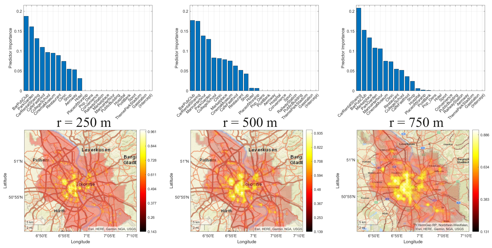
The maximum radius
r has a direct influence on the results of the regression. A comparison of the regression results with varying radius is carried out in
Figure A1. In order to compare the results of the regression analysis, the distances
are normalized with the maximum boundary. The graphs show small differences in the importance and ranking of categories for
r = 250 m and 500 m. At a distance of 750 m, the results deviate somewhat more clearly from the other distances. However, for all for cases the predictor importances are in the same order of magnitude. A similar picture emerges for the heat maps. With larger distance a lower resolution results whereby sharp demarcations between the attractiveness values are no longer recognizable. However, with smaller distance the computation time for the generation of the heat maps increases. Therefore a value of
r = 500 m seems a good trade off between accuracy and computation time. Comparing the obtained attractiveness values reveals also only small differences, so that the results of the genetic optimization are not affected.
Figure A1.
(Top): Predictor estimates of the linear regression for different values of r. The values are normalized for comparison. (Bottom): Example heat maps of cologne for different r.
Figure A1.
(Top): Predictor estimates of the linear regression for different values of r. The values are normalized for comparison. (Bottom): Example heat maps of cologne for different r.
References
- Gkatzoflias, D.; Drossinos, I.; Zubaryeva, A.; Zambelli, P.; Dilara, P.; Thiel, C. Optimal allocation of electric vehicle charging infrastructure in cities and regions: Scientific analysis or review. JRC Rep. 2016, 38, 1018–5593. [Google Scholar] [CrossRef]
- Baresch, M.; Moser, S. Allocation of e-car charging: Assessing the utilization of charging infrastructures by location. Transp. Res. Part Policy Pract. 2019, 124, 388–395. [Google Scholar] [CrossRef]
- Erbaş, M.; Kabak, M.; Özceylan, E.; Çetinkaya, C. Optimal siting of electric vehicle charging stations: A GIS-based fuzzy Multi-Criteria Decision Analysis. Energy 2018, 163, 1017–1031. [Google Scholar] [CrossRef]
- Pahlavanhoseini, A.; Sepasian, M.S. Scenario-based planning of fast charging stations considering network reconfiguration using cooperative coevolutionary approach. J. Energy Storage 2019, 23, 544–557. [Google Scholar] [CrossRef]
- Bryden, T.S.; Hilton, G.; Cruden, A.; Holton, T. Electric vehicle fast charging station usage and power requirements. Energy 2018, 152, 322–332. [Google Scholar] [CrossRef]
- Globisch, J.; Plötz, P.; Dütschke, E.; Wietschel, M. Consumer preferences for public charging infrastructure for electric vehicles. Transp. Policy 2019, 81, 54–63. [Google Scholar] [CrossRef]
- Krause, J.; Ladwig, S.; Saupp, L.; Horn, D.; Schmidt, A.; Schwalm, M. Perceived Usage Potential of Fast-Charging Locations. World Electr. Veh. J. 2018, 9, 14. [Google Scholar] [CrossRef] [Green Version]
- Hecht, C.; Das, S.; Bussar, C.; Sauer, D.U. Representative, empirical, real-world charging station usage characteristics and data in Germany. eTransportation 2020, 6, 100079. [Google Scholar] [CrossRef]
- Olk, C.; Trunschke, M.; Bussar, C.; Sauer, D.U. Empirical Study of Electric Vehicle Charging Infrastructure Usage in Ireland. In Proceedings of the 2019 4th IEEE Workshop on the Electronic Grid (eGRID), Xiamen, China, 14 November 2019; pp. 1–8. [Google Scholar] [CrossRef]
- Betz, J.; Walther, L.; Lienkamp, M. Analysis of the charging infrastructure for battery electric vehicles in commercial companies. In Proceedings of the 2017 IEEE Intelligent Vehicles Symposium (IV), Los Angeles, CA, USA, 11–14 June 2017; pp. 1643–1649. [Google Scholar] [CrossRef]
- Efthymiou, D.; Chrysostomou, K.; Morfoulaki, M.; Aifantopoulou, G. Electric vehicles charging infrastructure location: A genetic algorithm approach. Eur. Transp. Res. Rev. 2017, 9, 596. [Google Scholar] [CrossRef] [Green Version]
- Ji, D.; Zhao, Y.; Dong, X.; Zhao, M.; Yang, L.; Lv, M.; Chen, G. A Spatial-Temporal Model for Locating Electric Vehicle Charging Stations. In Embedded Systems Technology; Bi, Y., Chen, G., Deng, Q., Wang, Y., Eds.; Springer: Singapore, 2018; Volume 857, pp. 89–102. [Google Scholar] [CrossRef]
- Cocca, M.; Giordano, D.; Mellia, M.; Vassio, L. Data Driven Optimization of Charging Station Placement for EV Free Floating Car Sharing. In Proceedings of the 2018 21st International Conference on Intelligent Transportation Systems (ITSC), Maui, HI, USA, 4–7 November 2018; pp. 2490–2495. [Google Scholar] [CrossRef]
- Wagner, S.; Götzinger, M.G.; Neumann, D. Optimal Location of Charging Stations in Smart Cities: A point of Interest Based Approach. In Proceedings of the Thirty Fourth International Conference on Information Systems, Milan, Italy, 15–18 December 2013; Volume 3. [Google Scholar]
- Schmidt, M.; Zmuda-Trzebiatowski, P.; Kiciński, M.; Sawicki, P.; Lasak, K. Multiple-Criteria-Based Electric Vehicle Charging Infrastructure Design Problem. Energies 2021, 14, 3214. [Google Scholar] [CrossRef]
- Mortimer, B.J.; Bach, A.D.; Hecht, C.; Sauer, D.U.; De Doncker, R.W. Public Charging Infrastructure in Germany—A Utilization and Profitability Analysis. J. Mod. Power Syst. Clean Energy 2021, 99, 1–10. [Google Scholar] [CrossRef]
- Wolbertus, R.; van den Hoed, R.; Maase, S. Benchmarking Charging Infrastructure Utilization. World Electr. Veh. J. 2016, 8, 754–771. [Google Scholar] [CrossRef] [Green Version]
- GitHub-Merten Peetz MorbZ. OsmPoisPbf: Extracts All POIs from an OpenStreetMap File and Outputs These in a Comma Seperated File. Available online: https://github.com/MorbZ/OsmPoisPbf (accessed on 27 April 2022).
- Robusto, C.C. The Cosine-Haversine Formula. Am. Math. Mon. 1957, 64, 38. [Google Scholar] [CrossRef]
- Virtanen, P.; Gommers, R.; Oliphant, T.E.; Haberland, M.; Reddy, T.; Cournapeau, D.; Burovski, E.; Peterson, P.; Weckesser, W.; Bright, J.; et al. SciPy 1.0: Fundamental Algorithms for Scientific Computing in Python. Nat. Methods 2020, 17, 261–272. [Google Scholar] [CrossRef] [PubMed] [Green Version]
- Hunter, J.D. Matplotlib: A 2D graphics environment. Comput. Sci. & Eng. 2007, 9, 90–95. [Google Scholar] [CrossRef]
- The Python Package Index (PyPI). Geneticalgorithm 1.0.2. Available online: https://pypi.org/project/geneticalgorithm/ (accessed on 6 March 2022).
- Hotelling, H. Stability in Competition. Econ. J. 1929, 39, 41. [Google Scholar] [CrossRef]
- Dyke, K.J.; Schofield, N.; Barnes, M. The Impact of Transport Electrification on Electrical Networks. IEEE Trans. Ind. Electron. 2010, 57, 3917–3926. [Google Scholar] [CrossRef]
- Dubey, A.; Santoso, S. Electric Vehicle Charging on Residential Distribution Systems: Impacts and Mitigations. IEEE Access 2015, 3, 1871–1893. [Google Scholar] [CrossRef]
- Lopes, J.A.P.; Soares, F.J.; Almeida, P.M.R. Integration of Electric Vehicles in the Electric Power System. Proc. IEEE 2011, 99, 168–183. [Google Scholar] [CrossRef] [Green Version]
- Anwar, M.B.; Muratori, M.; Jadun, P.; Hale, E.; Bush, B.; Denholm, P.; Ma, O.; Podkaminer, K. Assessing the value of electric vehicle managed charging: A review of methodologies and results. Energy & Environ. Sci. 2022, 15, 466–498. [Google Scholar] [CrossRef]
- Hecht, C.; Figgener, J.; Sauer, D.U. ISEAview–Elektromobilität; ISEA Insitute, RWTH Aachen: Aachen, Germany, 2021. [Google Scholar]
| Publisher’s Note: MDPI stays neutral with regard to jurisdictional claims in published maps and institutional affiliations. |
© 2022 by the authors. Licensee MDPI, Basel, Switzerland. This article is an open access article distributed under the terms and conditions of the Creative Commons Attribution (CC BY) license (https://creativecommons.org/licenses/by/4.0/).


 ,
, 


