Formation and Control of Self-Sealing High Permeability Groundwater Mounds in Impermeable Sediment: Implications for SUDS and Sustainable Pressure Mound Management

Abstract
:
Contents
- 1.0
- Introduction
- 2.0
- Calculation Methodology used to Interpret Field Observations
- 2.1
- Overland Flow Rates
- 2.2
- Calculation of Recharge Volumes
- 2.3
- Design Storms
- 2.4
- Pressure Loading
- 2.5
- Intrinsic Permeability
- 2.5.1
- Vertical and Horizontal Permeability
- 2.6
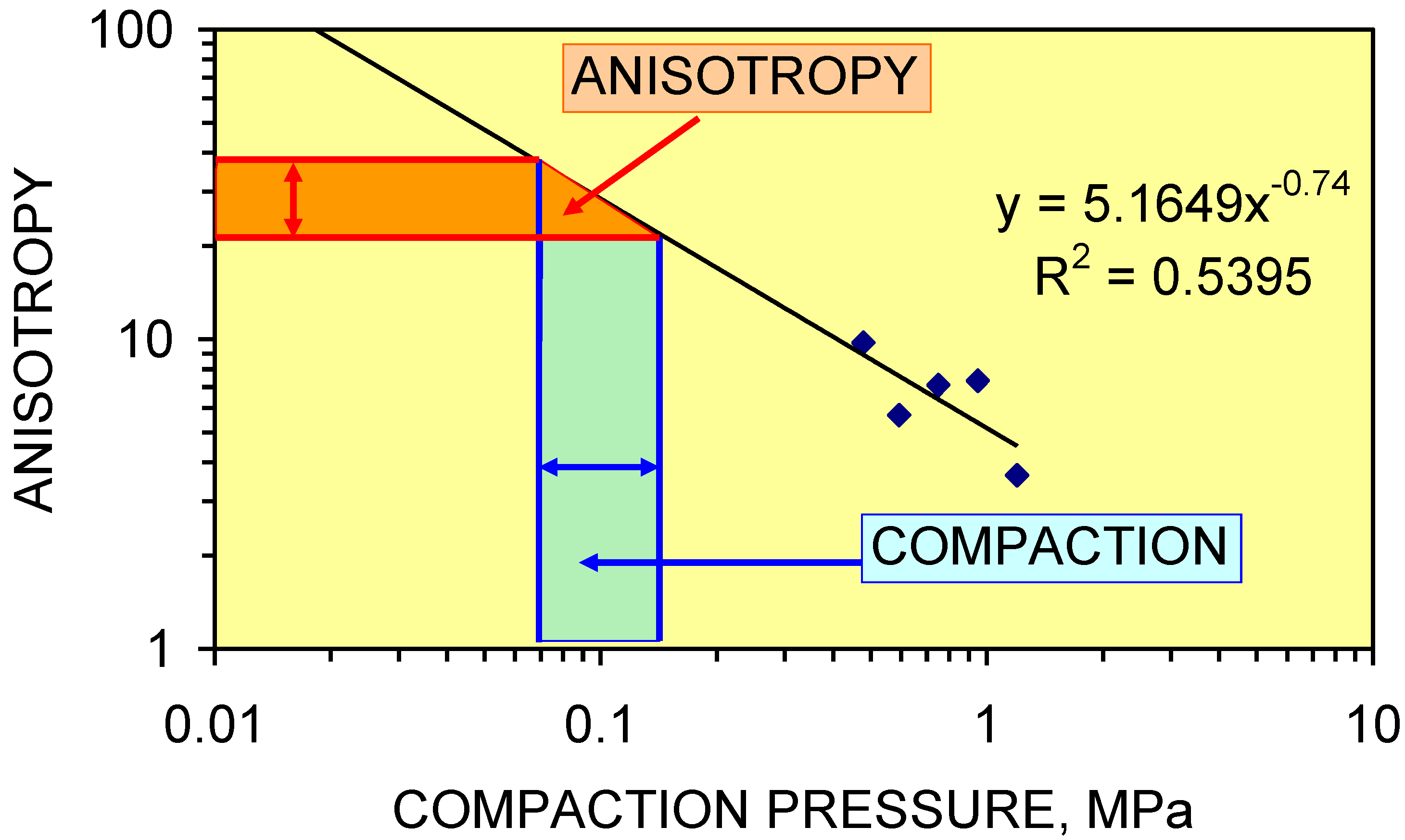
- Anisotropy
- 3.0
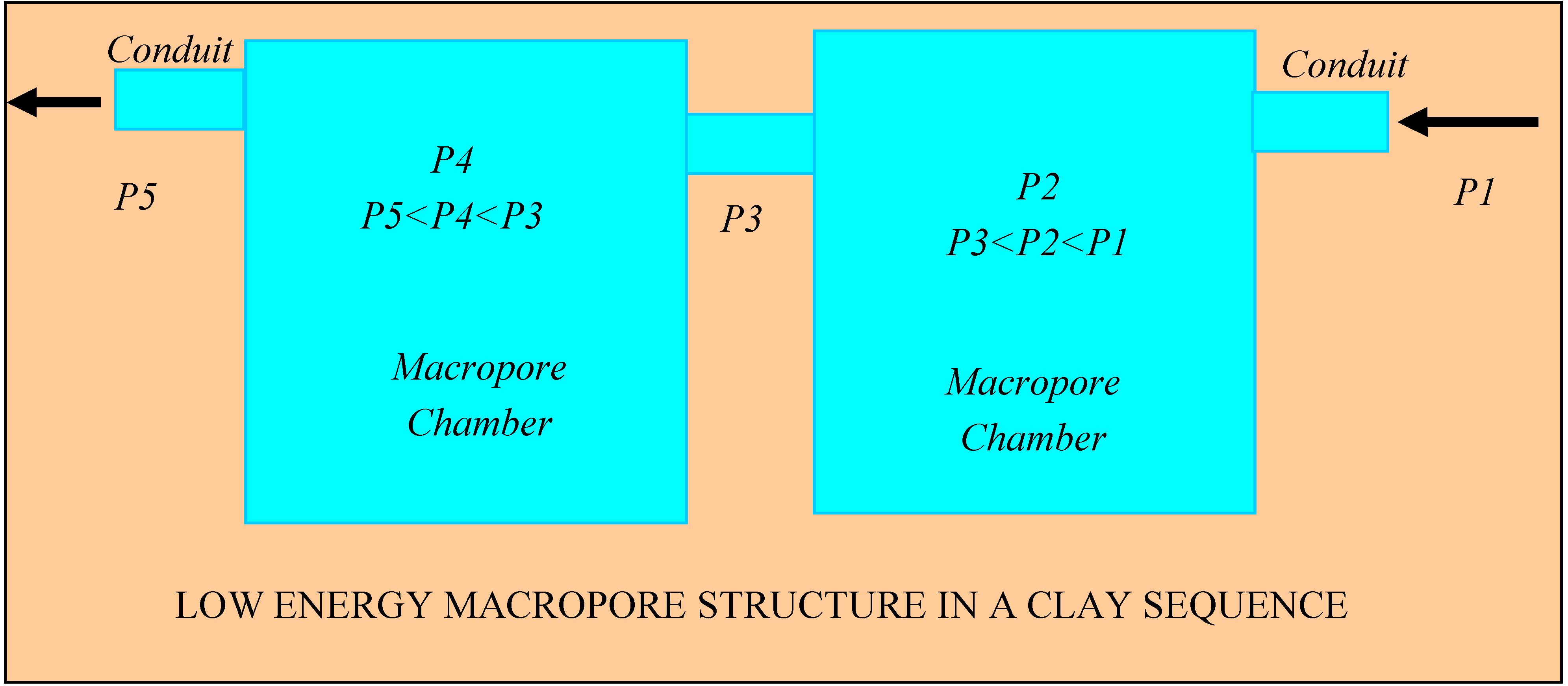
- Fluid Migration within a Groundwater Mound
- 3.1
- Analysis of Standing Water within a groundwater Mound
- 3.1.1
- Field Observations
- 3.1.2
- Interpreted Pore Throat Radii
- 3.2
- Pore Throat Reduction Mechanisms within the Groundwater Mound
- 3.2.1
- Pore Throat Reduction Associated with Bridging
- 3.2.2
- Flow Cessation Associated with Toroidal Bridges
- 3.2.2.1
- Toroidal Bridges in Unconsolidated Sand
- 3.2.2.2
- Toroidal Bridges in Winnowed Sand within a “natural pipe” derived from Greenloaning Till
- 3.2.2.3
- Toroidal Bridge Formation in Propagating Macropores within Greenloaning Lodgment Till
- 3.2.3
- Flow Cessation Associated with Hydration of Inter-Layer Porosity
- 3.2.4
- Other Flow Cessation Factors
- 3.2.5
- Standing Water-Model Summary
- 3.3
- Macropore Formation
- 3.3.1
- Sand Accumulations within Macropores/Natural Pipes
- 3.3.2
- Intrinsic Permeability within Macropores/Natural Pipes
- 3.3.3
- Flow Regimes around a Macropore
- 3.3.4
- Flow from the Macropore into the Surrounding Formation
- 4.0
- Groundwater Mound Envelope
- 4.1
- Pore Tortuosity at the Mound Boundary
- 4.2
- Equilibrium Mound Widths
- 4.3
- Groundwater Mound Growth as a Function of Time
- 4.4
- Impact of Pressure Losses on Groundwater Mound Diameter
- 4.5
- Seepage Volumes Associated with Groundwater Mounds
- 4.5.1
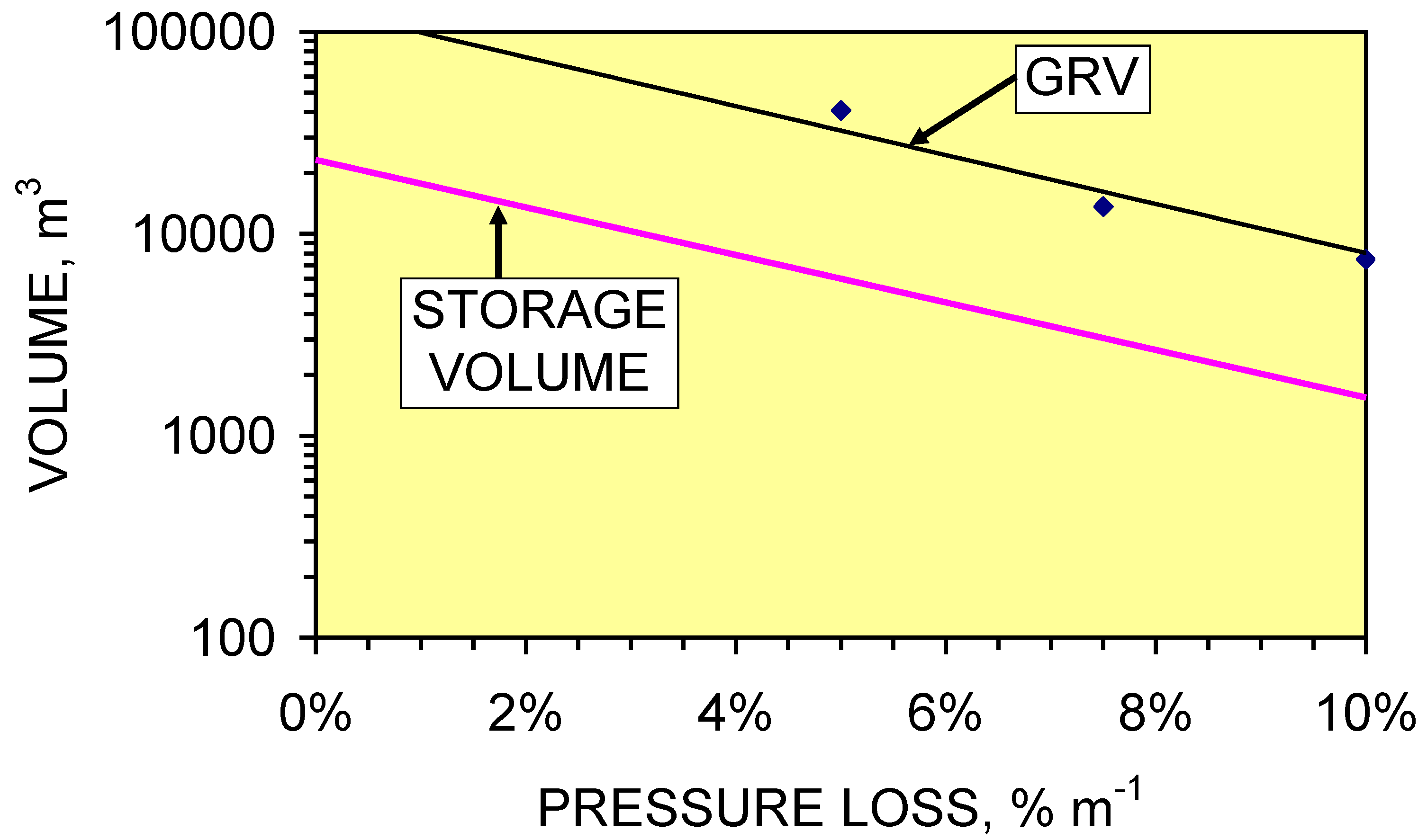
- Groundwater Mound Storage Volumes
- 4.5.2
- Seepage Volumes
- 5.0
- Modeling a Groundwater Mound for Storage
- 5.1
- Upper Surface of the Groundwater Mound: Dupuit Model
- 5.2
- Upper Surface of the Groundwater Mound: Macropore Propagation Model
- 5.3
- Lower Surface of the Groundwater Mound: Dupuit Model
- 5.4
- Macropore Analysis of the Lower Surface of the Groundwater Mound
- 5.5
- 3D Mound Volume and Assessment of Potential Resource
- 5.6
- Net Storage Volume
- 5.6.1
- Changes in Storage Capacity with Time
- 5.7
- Potential Resource
- 6.0
- Extraction of Water from a Groundwater Mound
- 6.1
- Water Quality
- 7.0
- Comparison of Observed Results with a Traditional Groundwater Mound Model
- 7.1
- Expected Groundwater Mound Behavior: Arid Environment
- 7.2
- Expected Groundwater Mound Behavior: Modeling
- 8.0
- Conclusions
- Acknowledgements
- Appendix 1
- A.1
- Sustainable Urban Drainage Systems
- A.2
- Location Map and Details of the Greenloaning Study Area
- References
- List of Principal Abbreviations
1. Introduction

2. Calculation Methodology Used to Interpret Field Observations
2.1. Overland Flow Rates

2.2. Calculation of Recharge Volumes
2.3. Design Storms
2.4. Pressure Loading
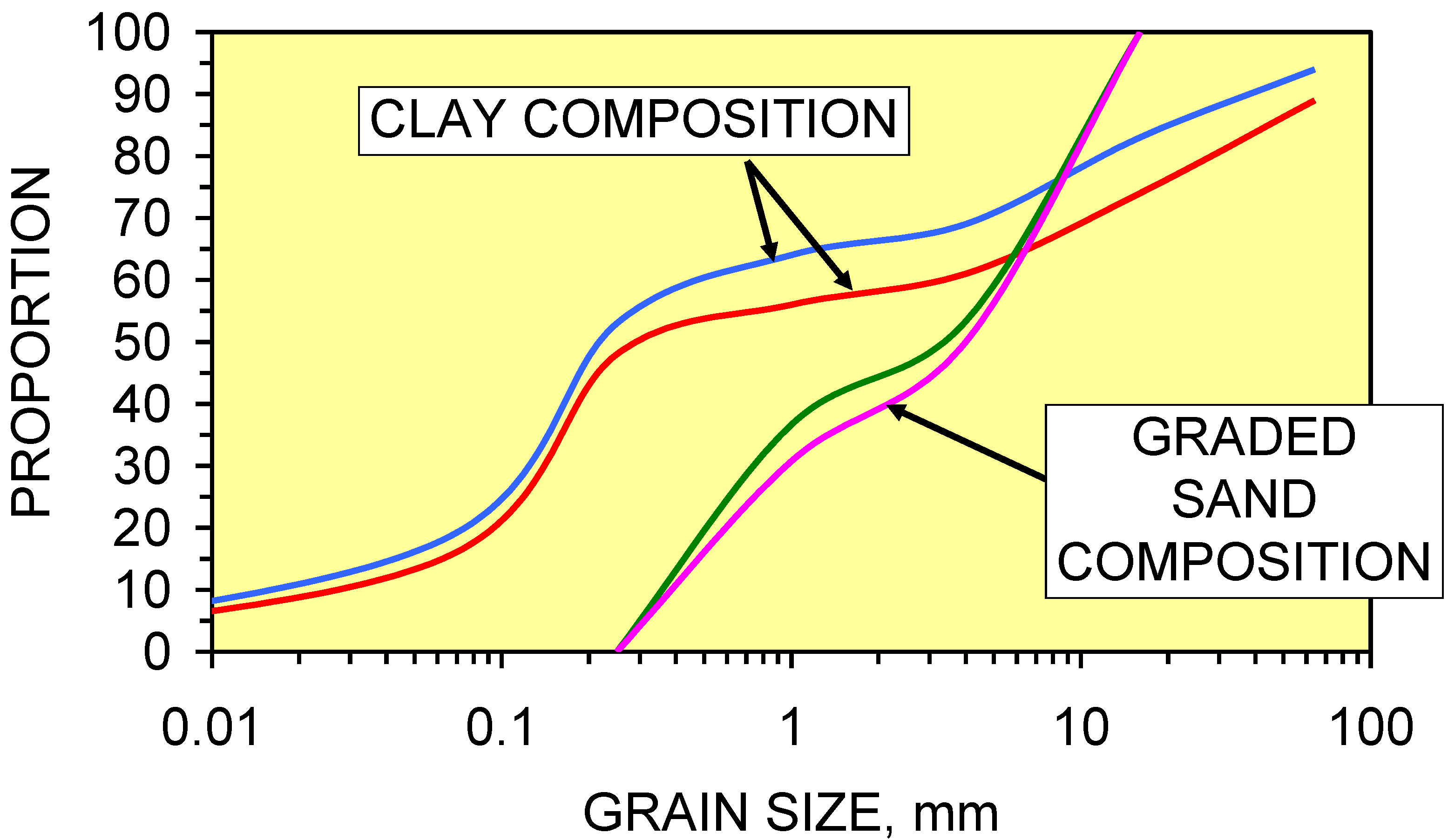
2.5. Intrinsic Permeability
2.5.1. Vertical and horizontal permeability
2.6. Anisotropy

3. Fluid Migration within a Groundwater Mound


3.1. Analysis of Standing Water within a Groundwater Mound
3.1.1. Field observations
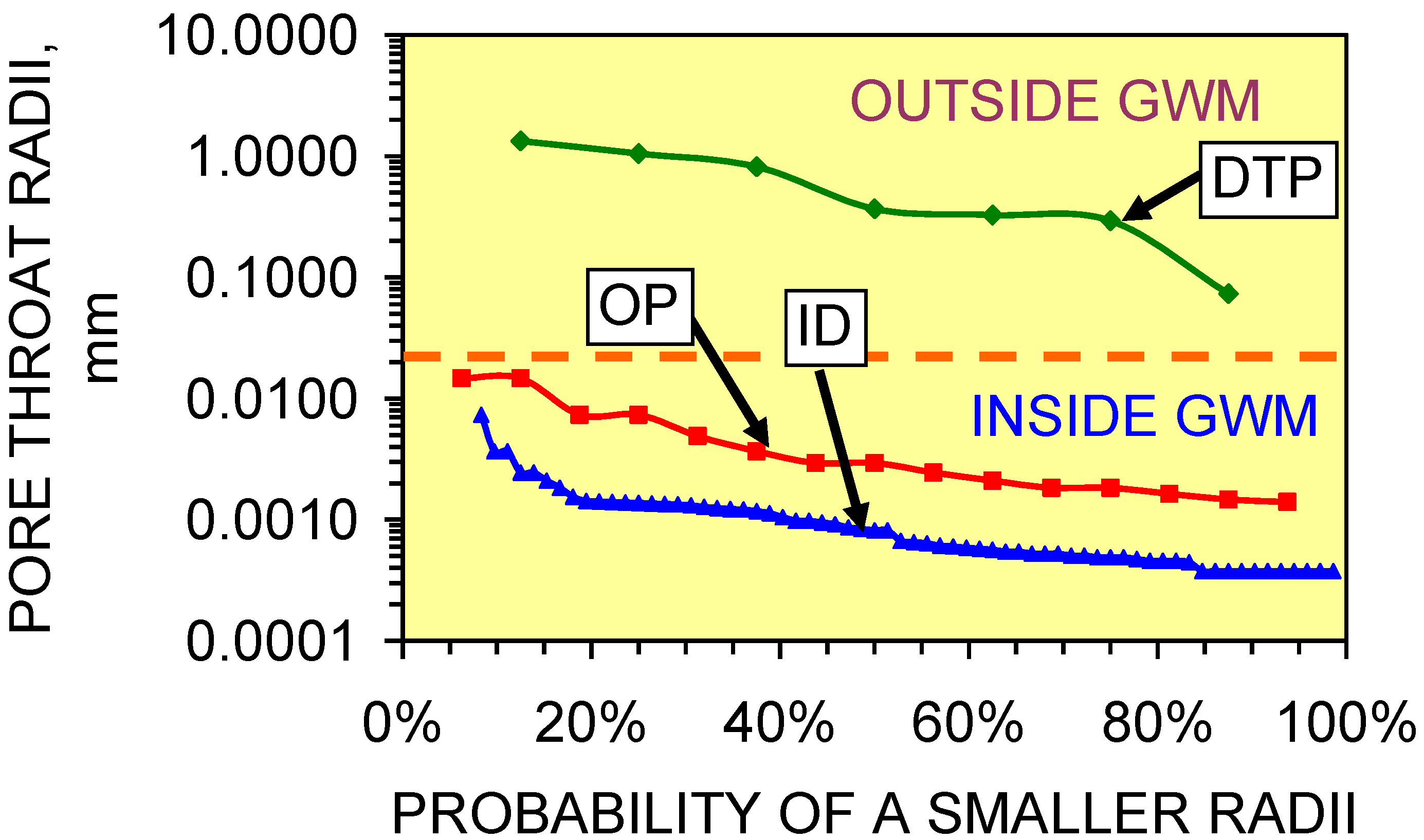
3.1.2. Interpreted pore throat radii

3.2. Pore Throat Reduction Mechanisms within the Groundwater Mound
3.2.1. Pore throat reduction associated with bridging

3.2.2. Flow cessation associated with toroidal bridges
- (i)
- an unconsolidated sand was placed in a water saturated tube and a driving force applied across the sand body. This experiment simulates the reactivation of flow within a sand filled natural pipe within the groundwater mound (Section 3.2.2.1);
- (ii)
- a sample of lodgment till was placed in a tube and fluidized. Clay particles were elutriated to create a simulated sand filled natural pipe. The tube was drained in order to simulate the lowering of the upper surface of the groundwater mound. The tube was then refilled with water and a driving force applied across the residual “winnowed sand” body to simulate the reactivation of a natural pipe during recharge (Section 3.2.2.2);
- (iii)
- a sample of lodgment till was placed in a tube and a gradually increasing driving force applied across the clay body in order to examine how macropores and natural pipes form (Section 3.2.2.3).
3.2.2.1. Toroidal bridges in unconsolidated sand
- (i)
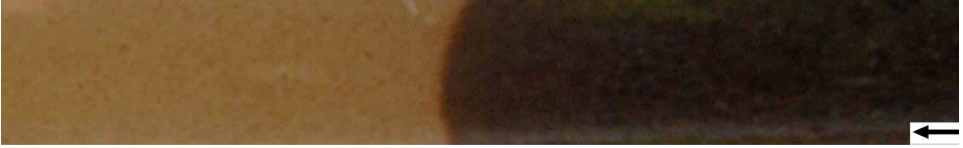
- In Figure 9a the initial recharge has separated the sand body to form two sand bodies separated by a water body. Fluid flow in the lower sand body is by fluidized flow within a zone of stationary particulates (expanded porosity) [40]. Stationary particulates are continuously moving particles in expanded porosity, where the upward force associated with the flowing water matches the downward gravitational force exerted by the particles [3,40]. Fluid flow in the upper sand body is within unexpanded inter-particle porosity. Rising air bubbles moving in the same direction as the water molecules coalesce (within the water body) and block the pores into the overlying sand body (i.e., create toroidal fluid bridges (Figure 8c)). The water flow leaving the upper sand body has a lower velocity than the water flow leaving the lower sand body. Over time the gap between the upper and lower sand bodies increases, as the upper sand body is pushed along the conduit by the force contained within the expanding water body.
- (ii)
- Figure 9b demonstrates that the water flow rate is sufficient to carry a few of the fluidized sand grains from the lower sand body into the overlying water column. This results in a counter flow of small sand particles rising in the main flow channel and descending in the adjacent slack water. The flow into the water body from the lower sand body will result in a loss of energy and a conversion of kinetic energy to potential energy. Continuing expansion of the water body volume with time, reflects an increase in potential energy pressure loading (Equation 3).
- (iii)
- Figure 9c shows that air has coalesced to form bubbles, which form toroidal bridges (Figure 8c). These toroidal bridges block entry to the pores in the overlying sand body. This results in:
- a reduction in the water flow rate through the upper sand body.
- a buildup of potential energy in the water body immediately downstream of the upper sand body.
- the rate of flow through the upper sand body decreasing as the volume of air bubbles along the infiltrating surface increases.

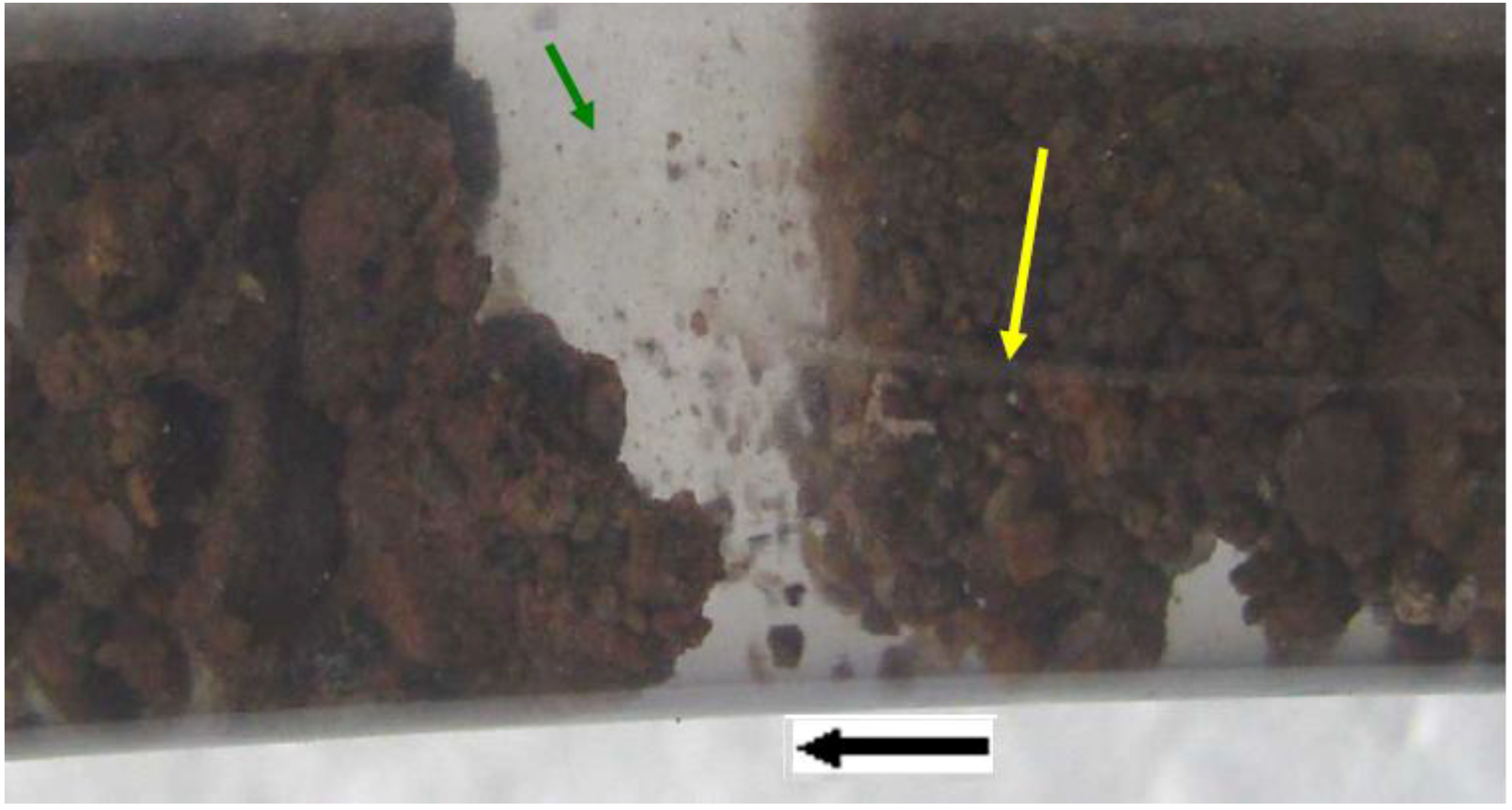
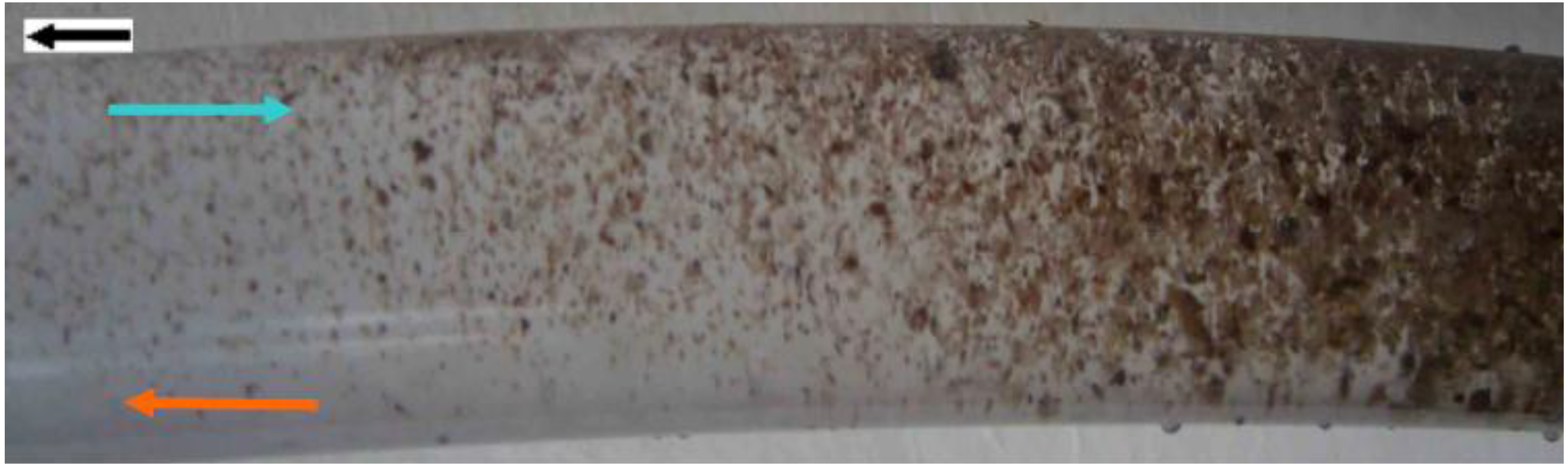
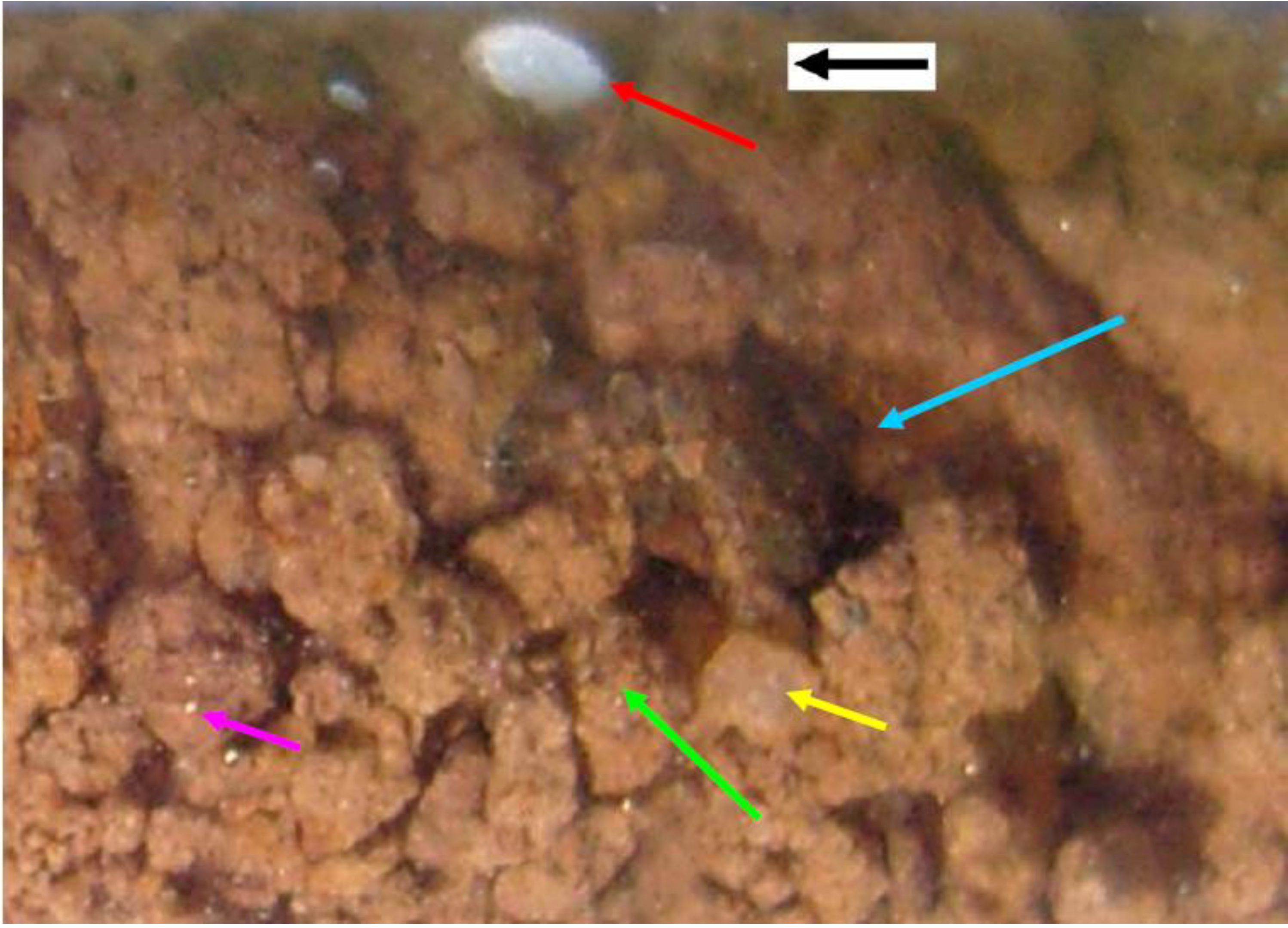
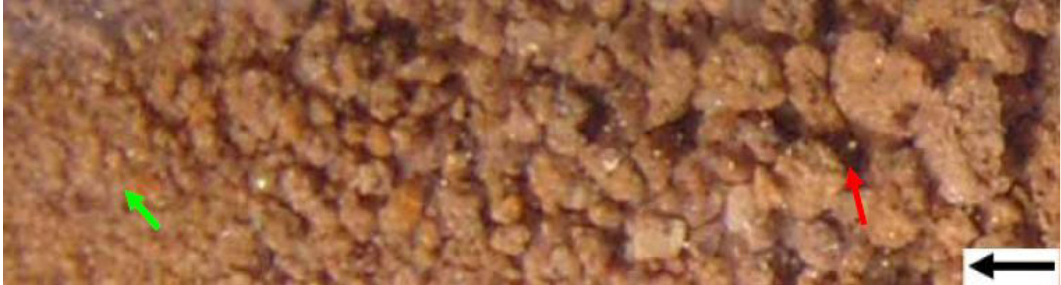
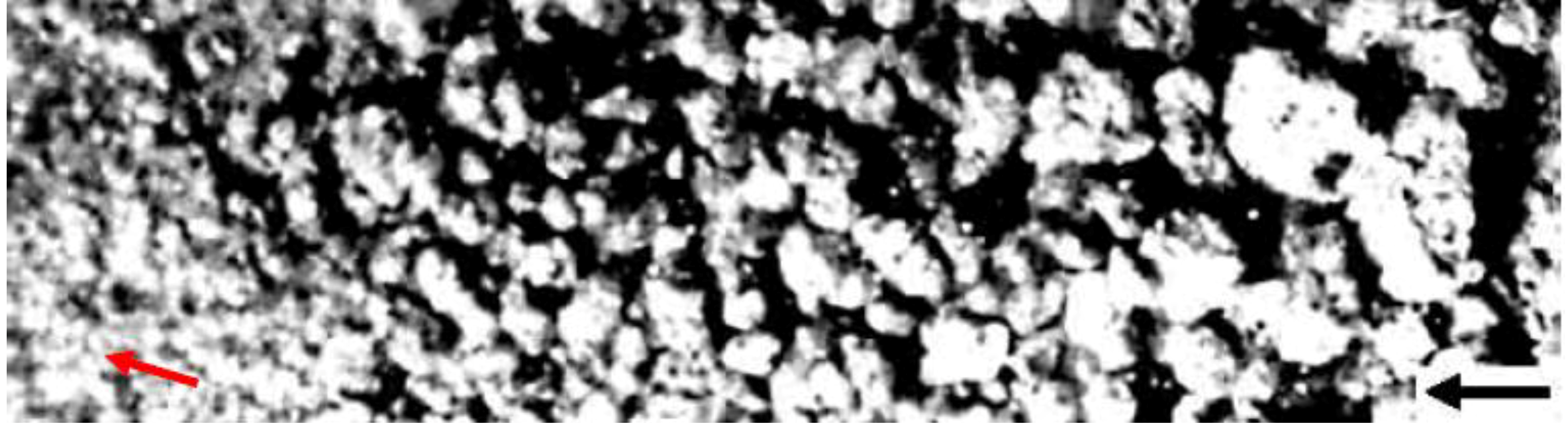
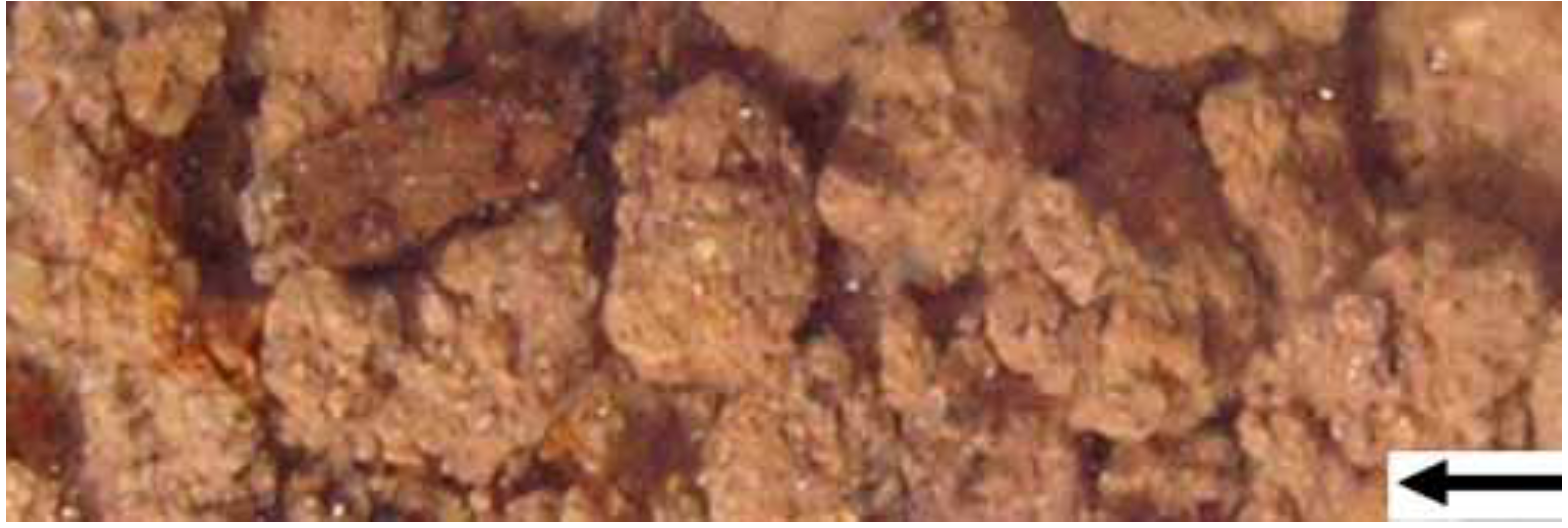
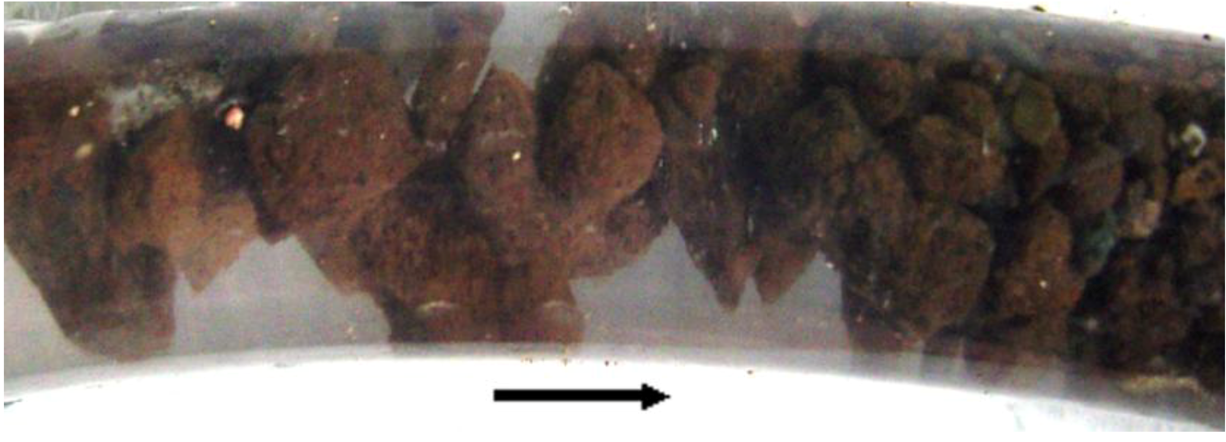
3.2.2.2. Toroidal bridges in winnowed sand within a “natural pipe” derived from Greenloaning till
- (i)
- Figure 10 demonstrates that the sediment column first breaks into a number of segments separated by expanding water bodies.
- (ii)
- After the water body reaches a critical size, the overlying sediment fluidizes and collapses into the water body (Figure 11).
- (iii)
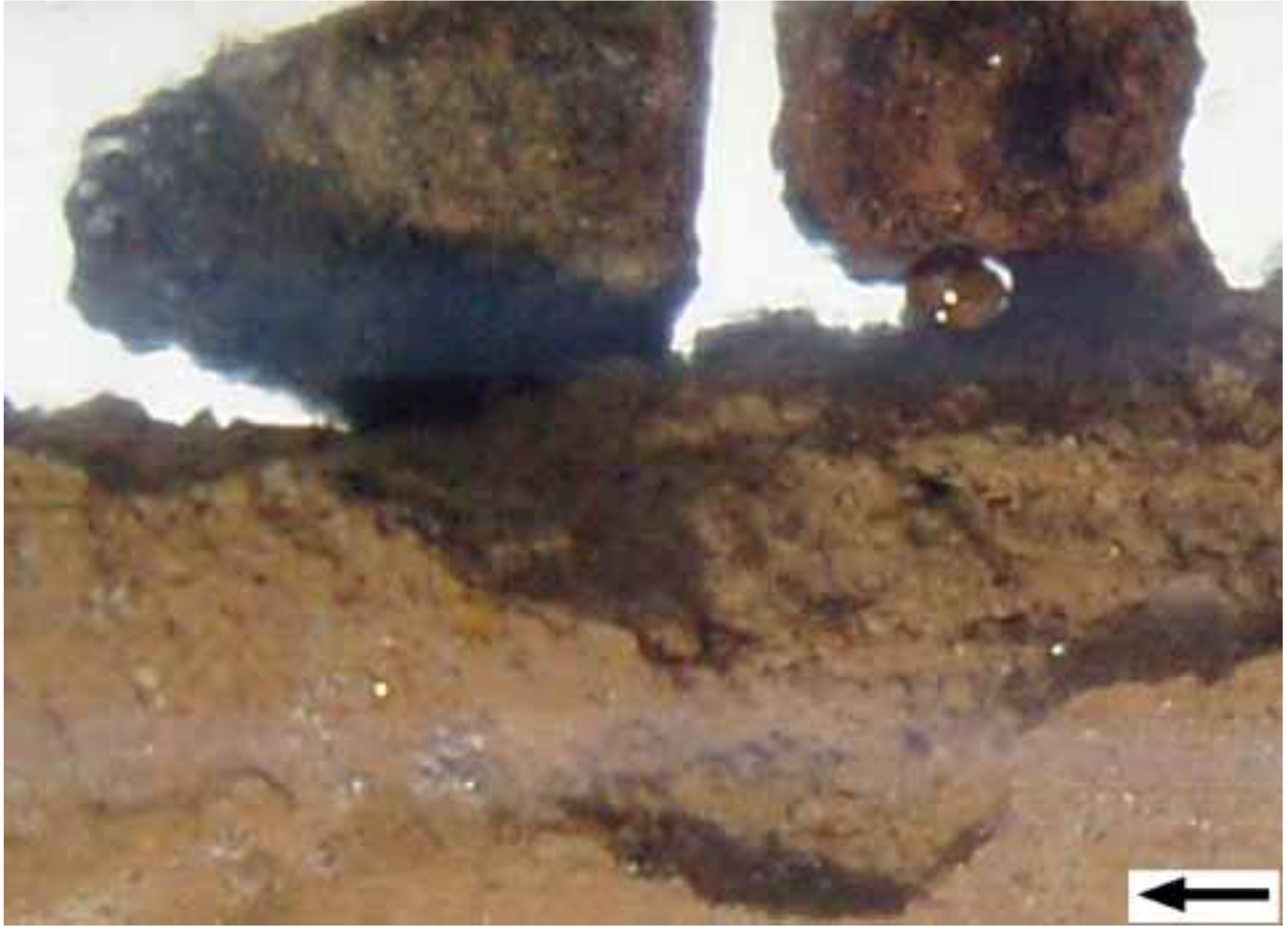
- (iv)
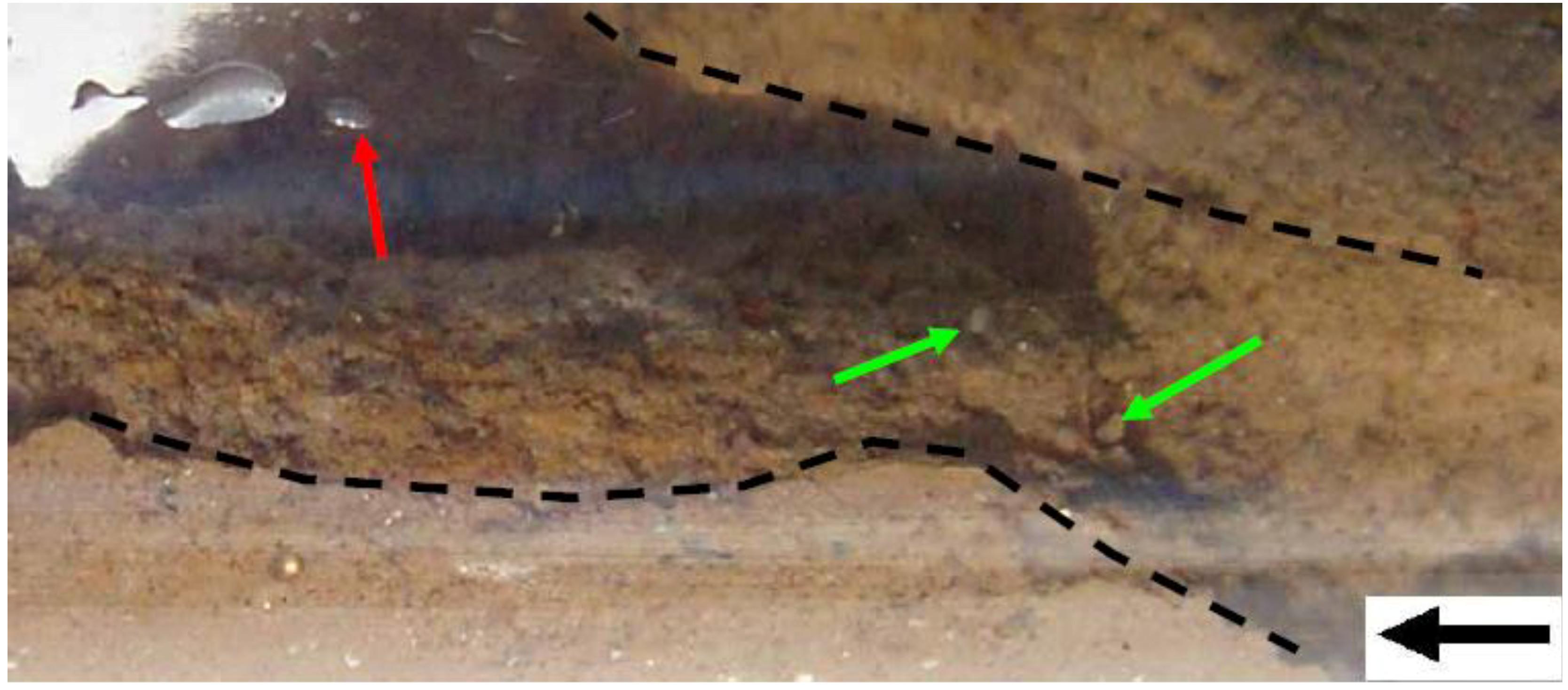
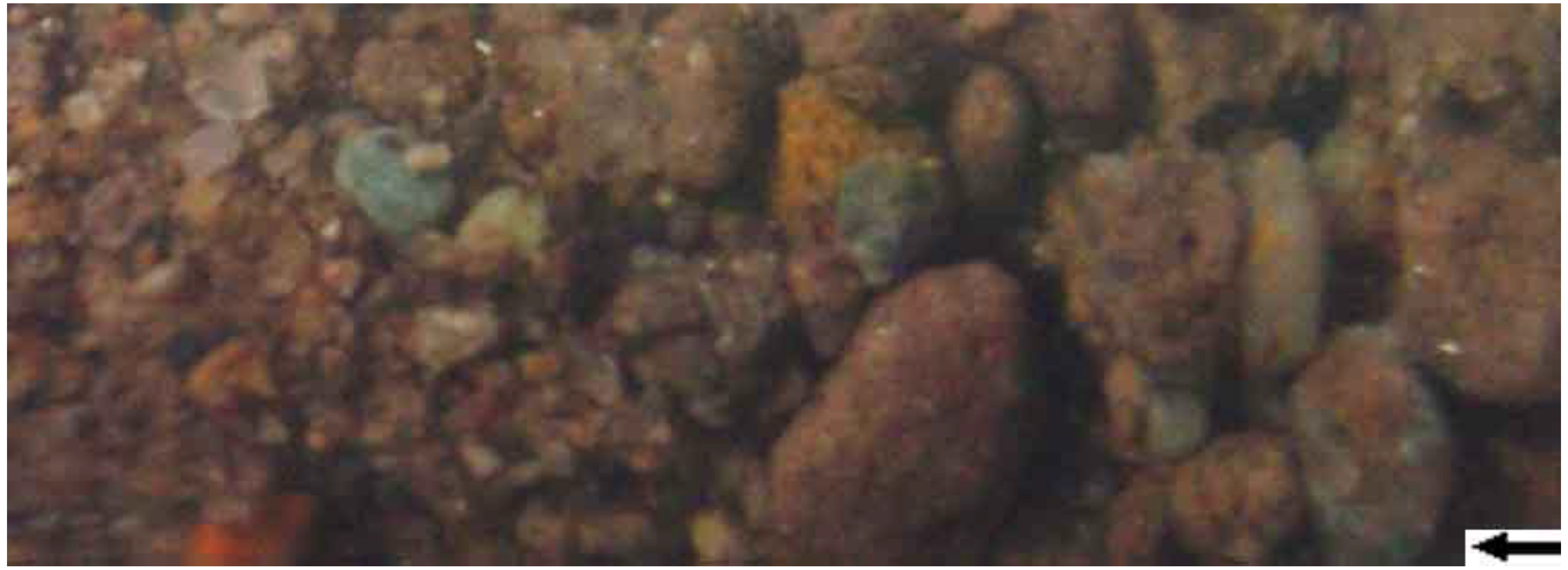
- Within the lower sediment body, nodular, irregular pores develop (white arrow (Figure 12)) which contain small discrete air bubbles. These expand over time (as they receive more air and water) to form discrete water bodies. The downstream surface of these enlarging pores is lined with air bubbles.
- (v)
- The main water body (Figure 10) is fed by a series of micro-tubes (yellow arrow (Figure 10 and Figure 12)), which are formed as a lining of nano-air bubbles. These water filled micro-tubes (<30 mm long) are fed with nano air bubbles through their base and sides. The nano bubbles coalesce towards the tube end to discharge a string of uniform sized air bubbles into the water body (Figure 12).
- (vi)
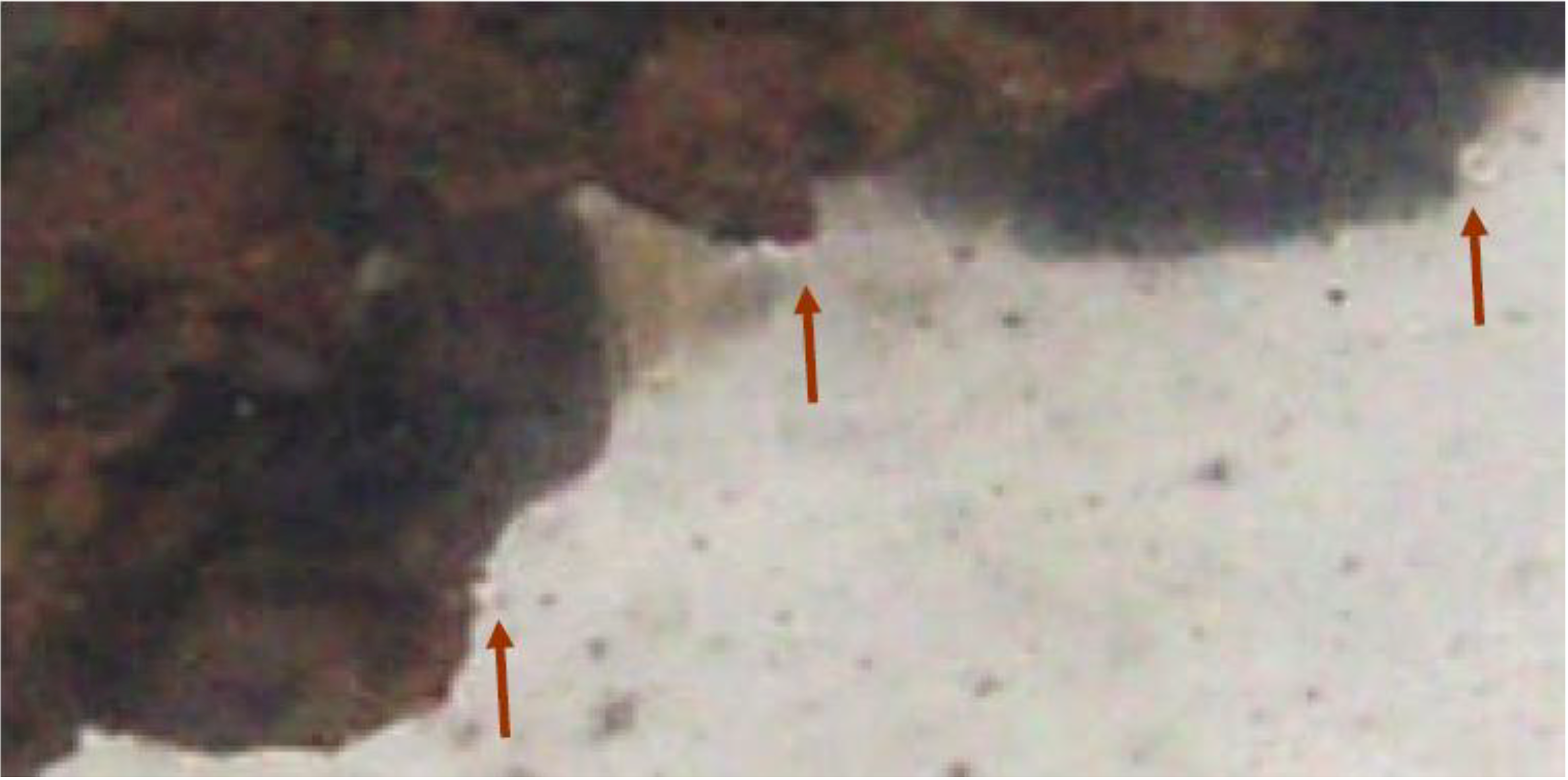
- The junction of the upper sediment body and the water body is marked (brown arrow) by a rim of nano and micro air bubbles (Figure 13). This is an analogous situation to that observed in Figure 9a,c. It indicates that the downstream surface of enlarging pores can be lined with air. These air bubbles reduce the sediment permeability at the junction of the pore and the sediment.


3.2.2.3. Toroidal bridge formation in propagating macropores within Greenloaning lodgment till


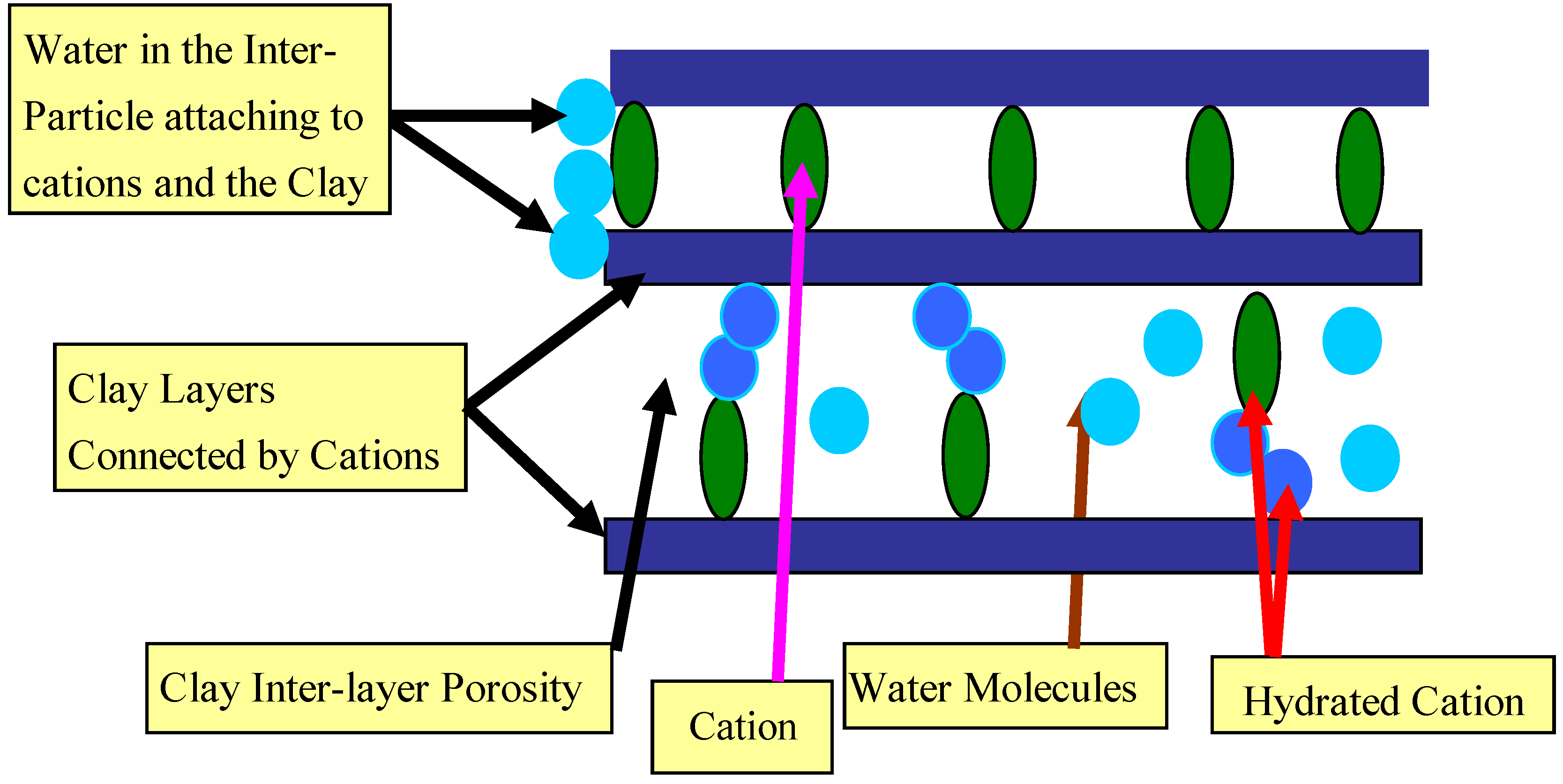
3.2.3. Flow cessation associated with hydration of the inter-layer porosity


3.2.4. Other flow cessation factors
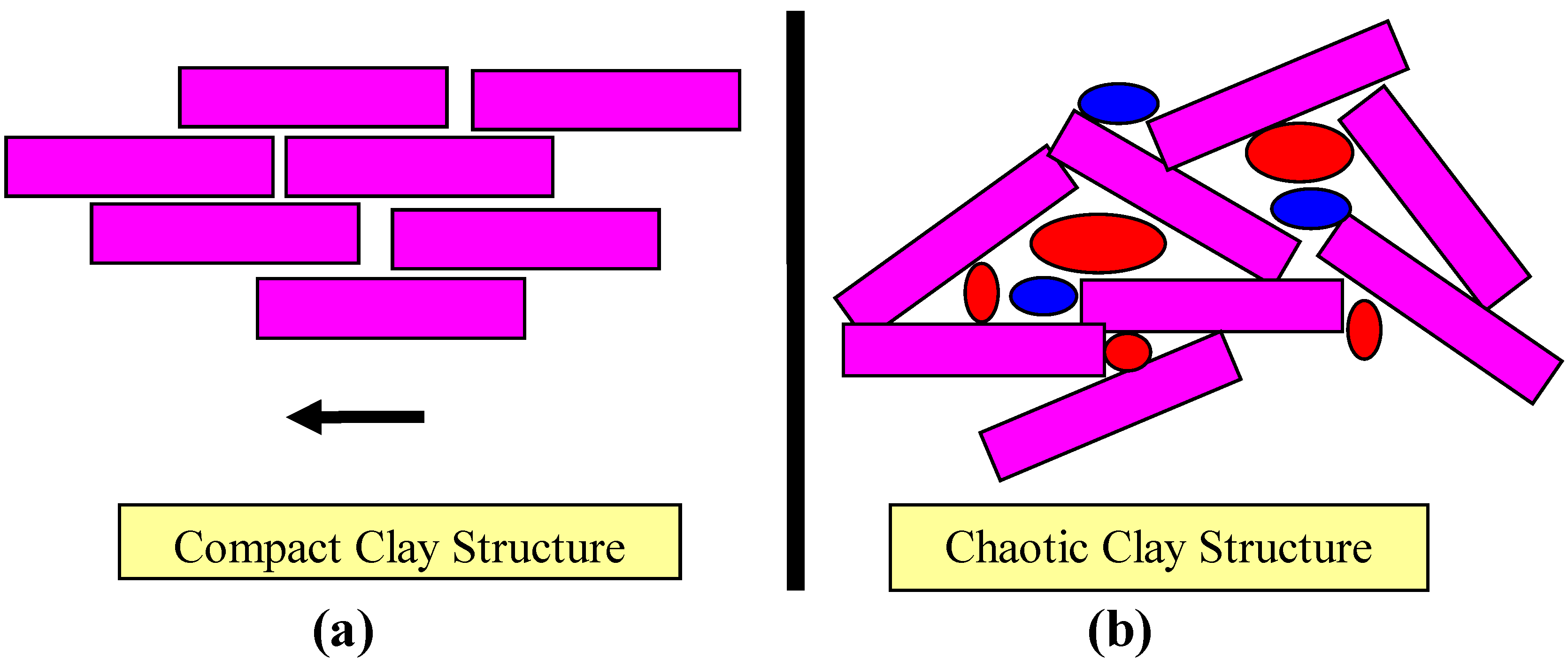
3.2.5. Standing water–model summary


3.3. Macropore Formation
- (i)
- the nodular or beaded macropore development at the end of the flow conduit is associated with pressure losses where each nodular pore represents an expanding store of energy, where kinetic energy is transferred to potential energy, and
- (ii)
- energy losses are accentuated along the downstream margins of the nodular pores by the formation of toroidal bridges associated with migrating air bubbles.
- (i)
- Low Driving Force: Inter-particle viscous flow through the clay. This results in the discharged water containing a high proportion of colloidal material (Figure 27). The presence of this colloidal material in the water moving ahead of the wetting front may have a surfactant effect and reduce θ (Equation 8).
- (ii)
- Medium Driving Force: Formation of beaded macropore pathways (containing clear water) separated by clay clods (Figure 28).
- (iii)
- (iv)
- Higher Driving Force: Formation of high permeability natural pipes (Figure 31).


3.3.1. Sand accumulations within macropores/natural pipes


3.3.2. Intrinsic permeability within macropores/natural pipes

3.3.3. Flow regimes around a macropore

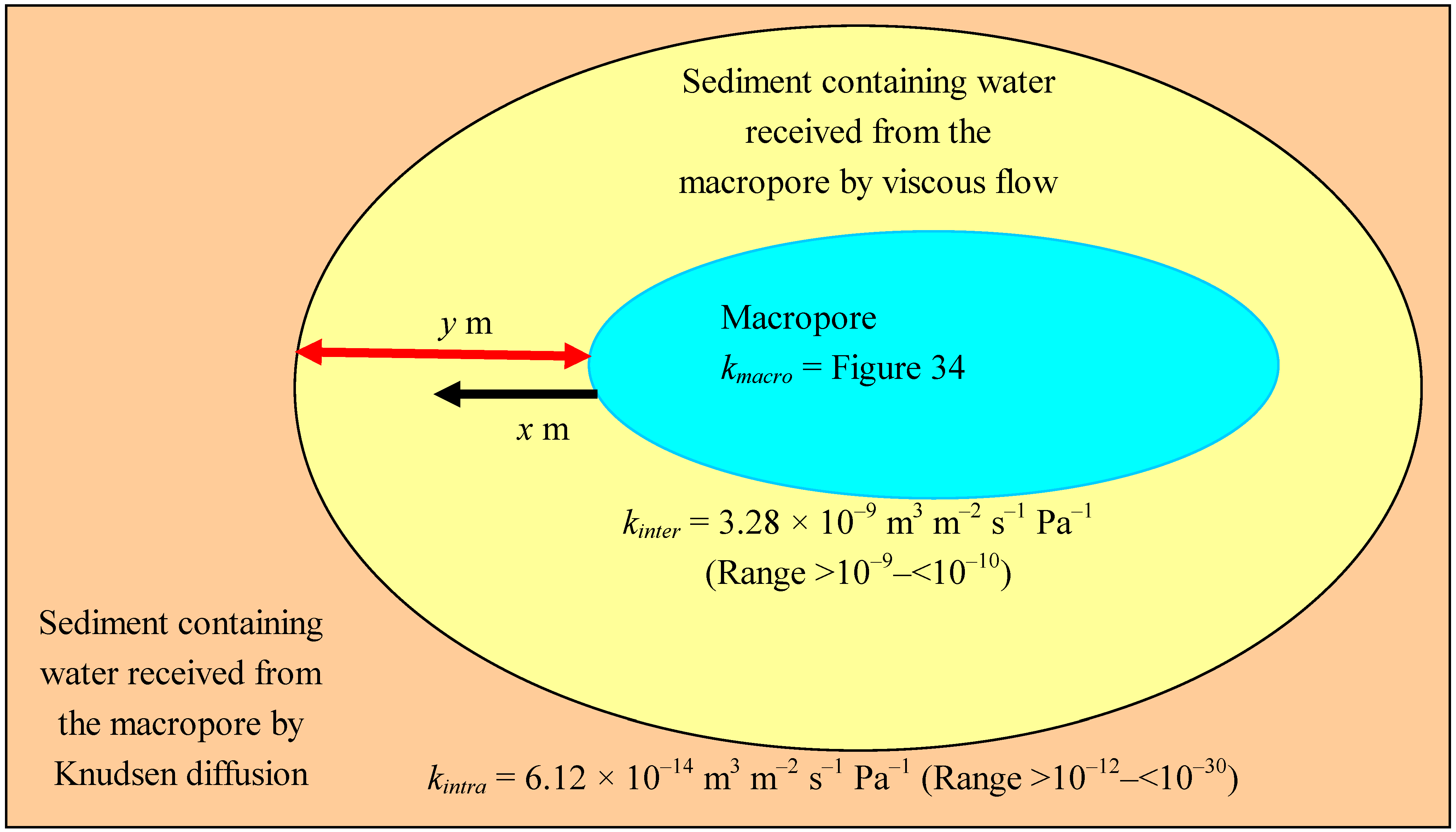
3.3.4. Flow from the macropore into the surrounding formation


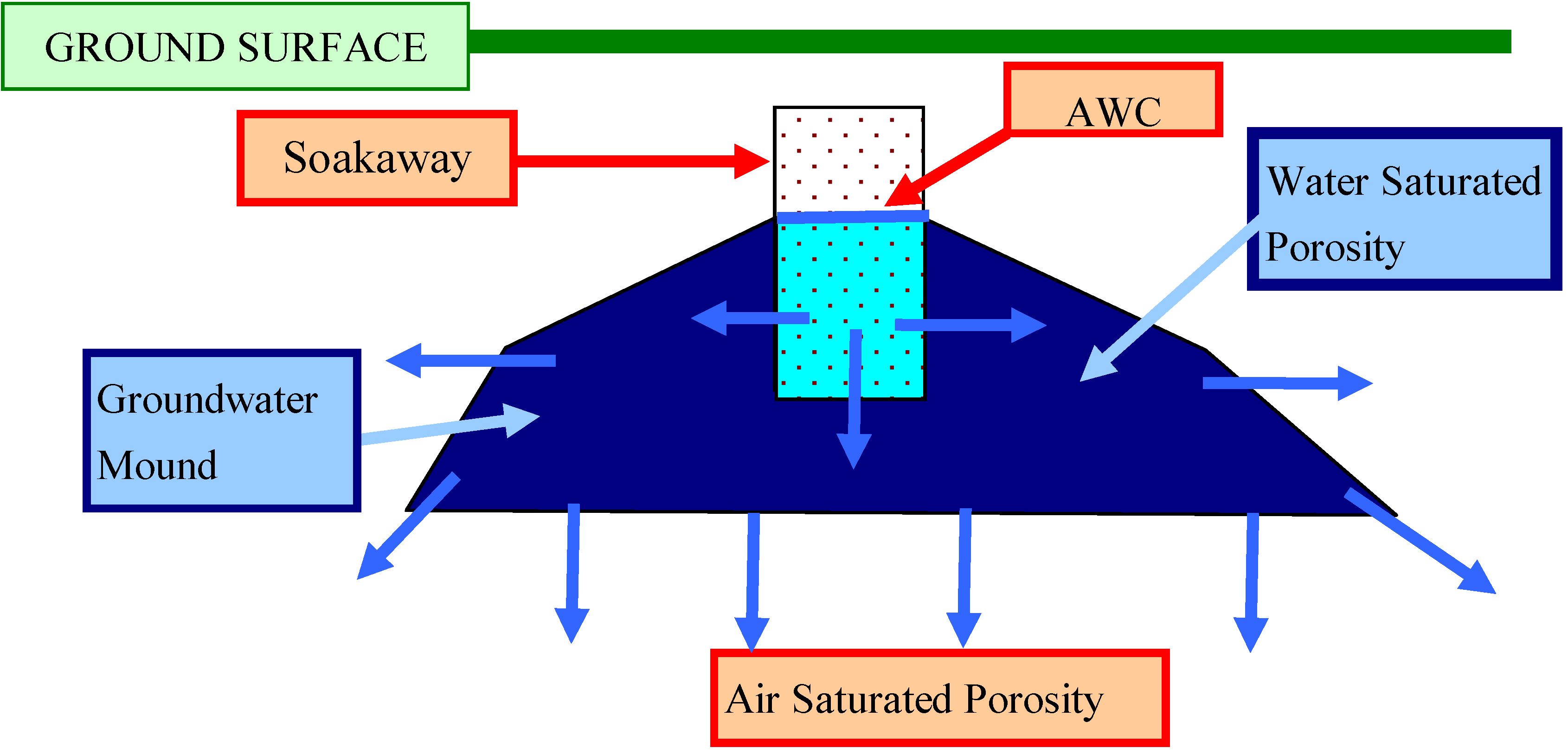
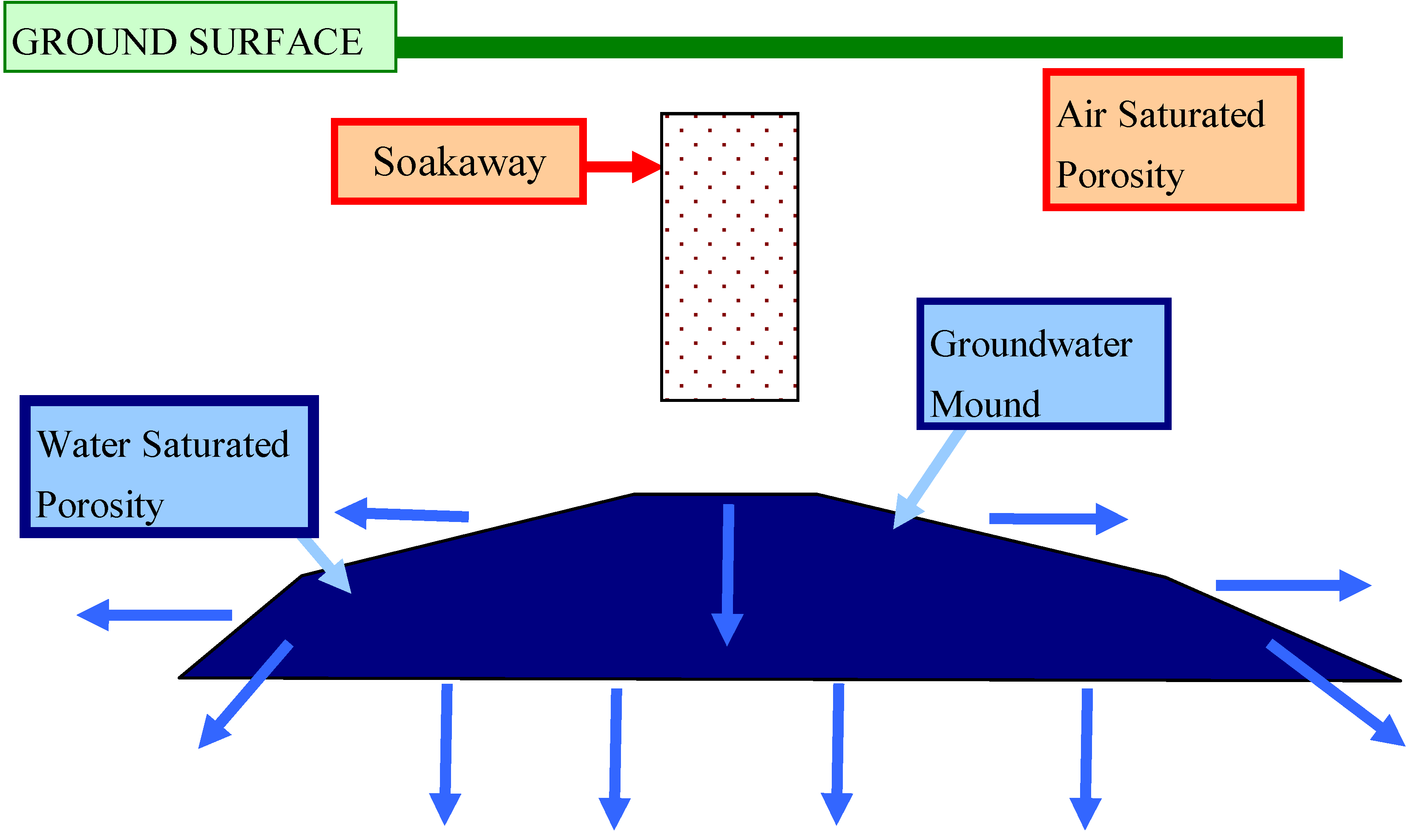
4. Groundwater Mound Envelope

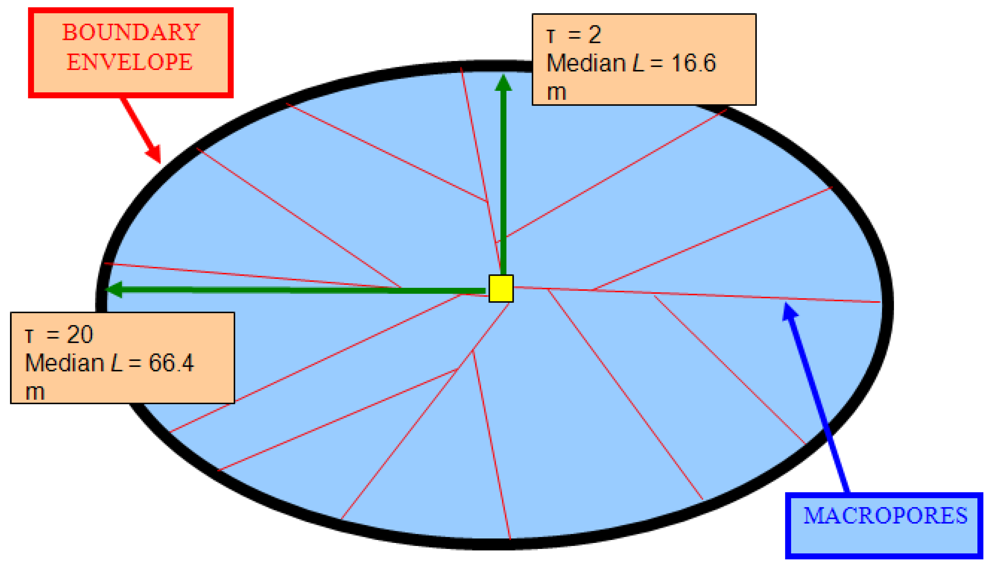
4.1. Pore Tortuosity at the Mound Boundary
4.2. Equilibrium Mound Widths


4.3. Groundwater Mound Growth as a Function of Time

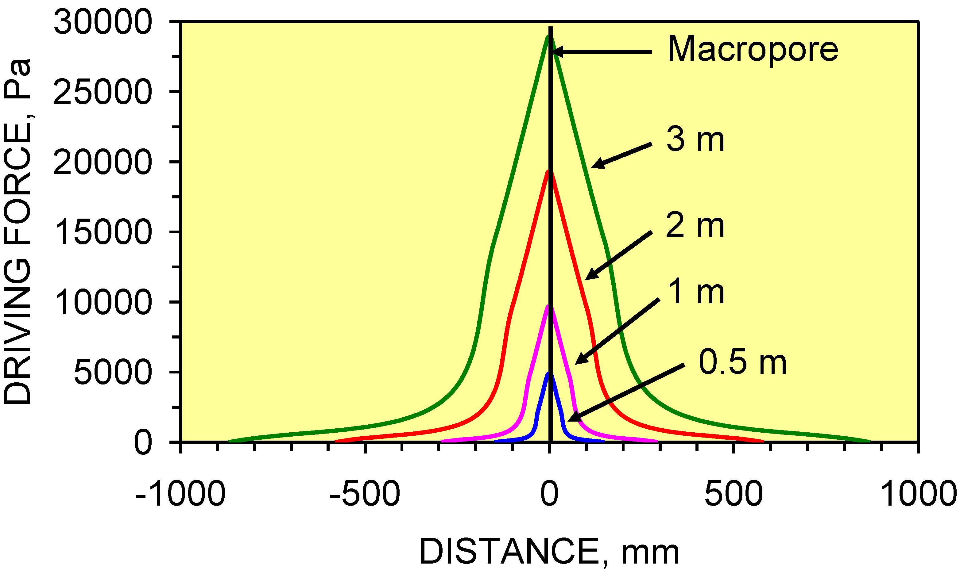
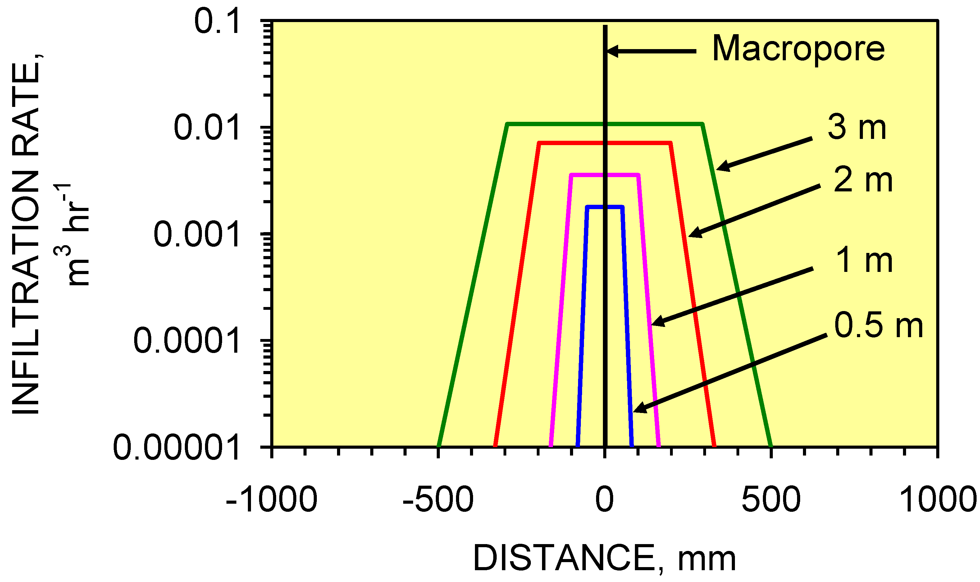
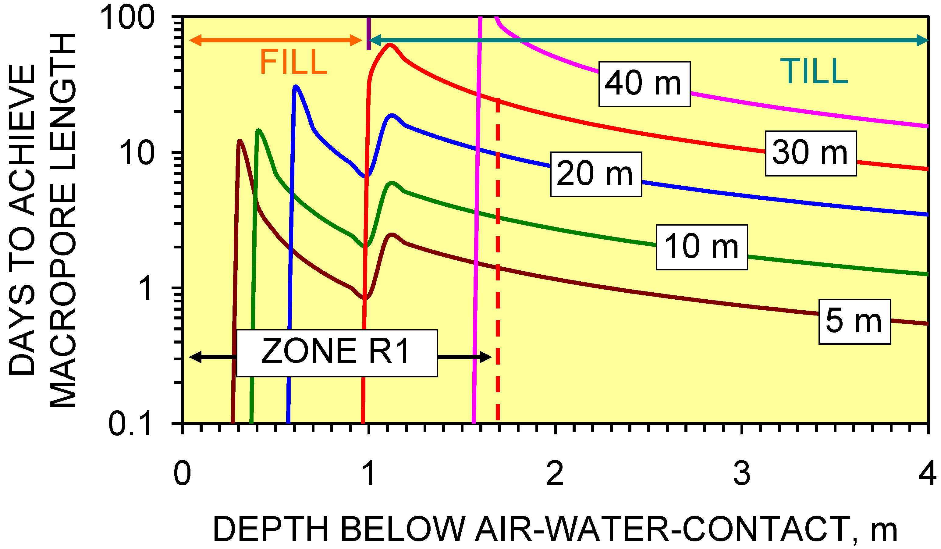
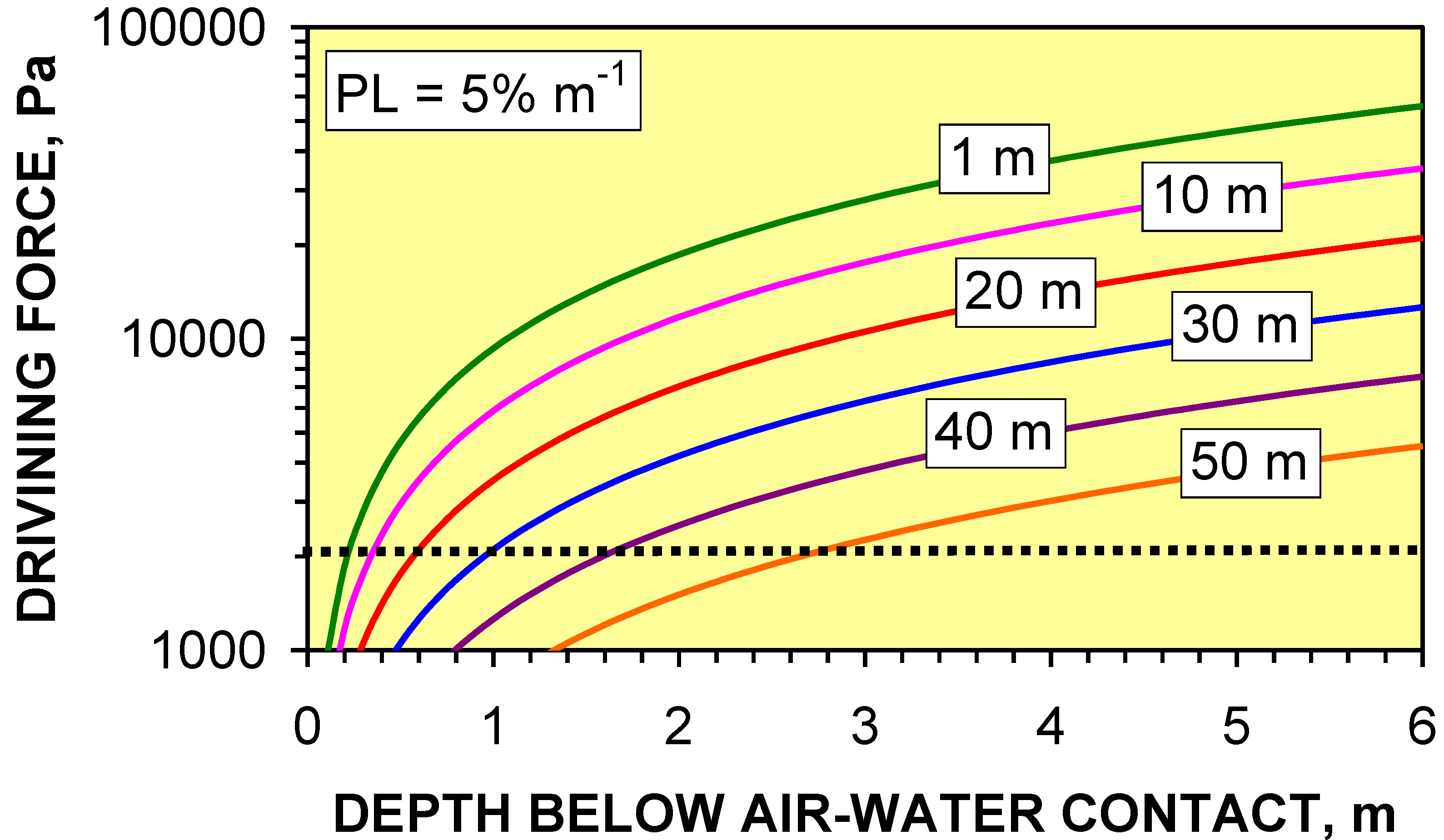
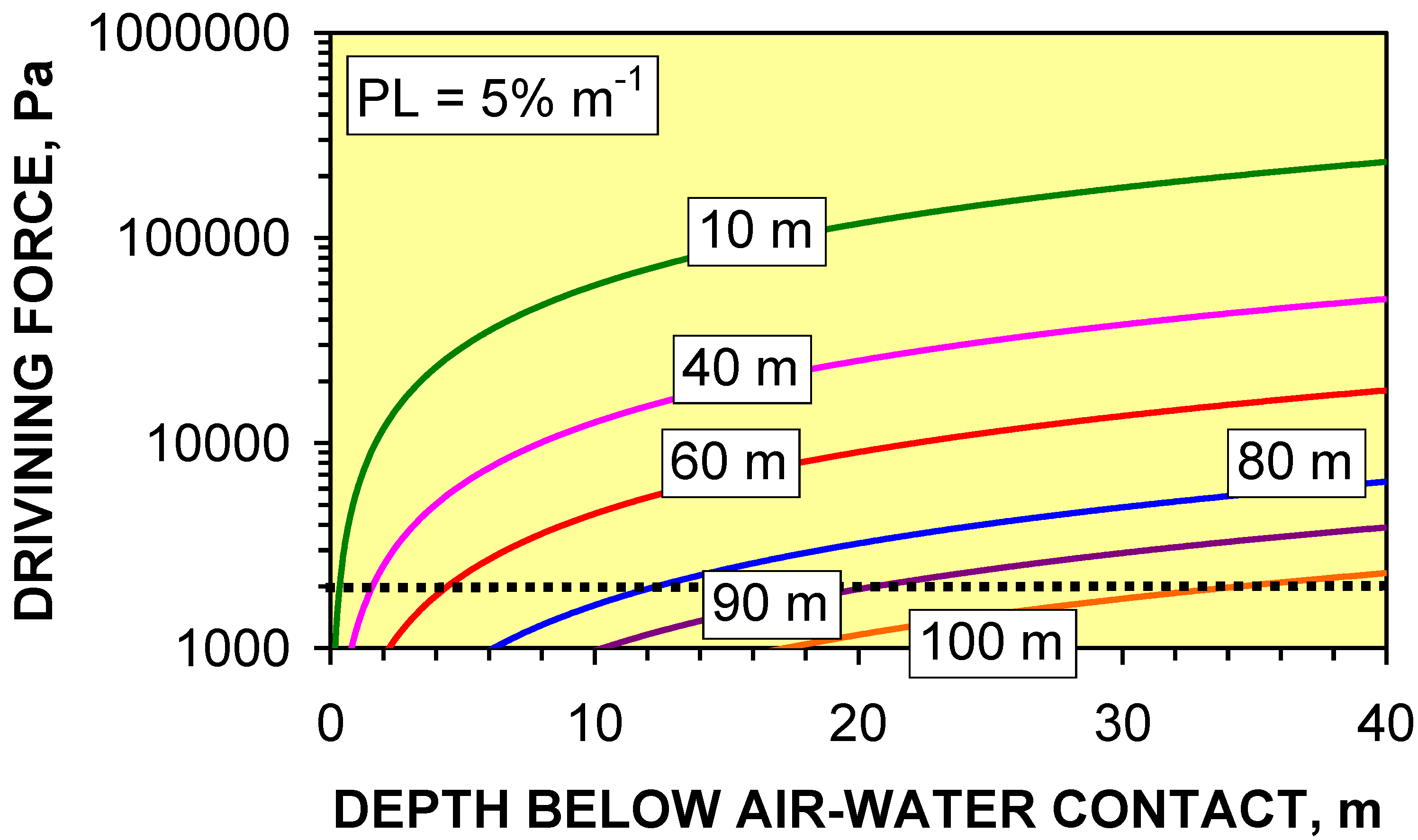
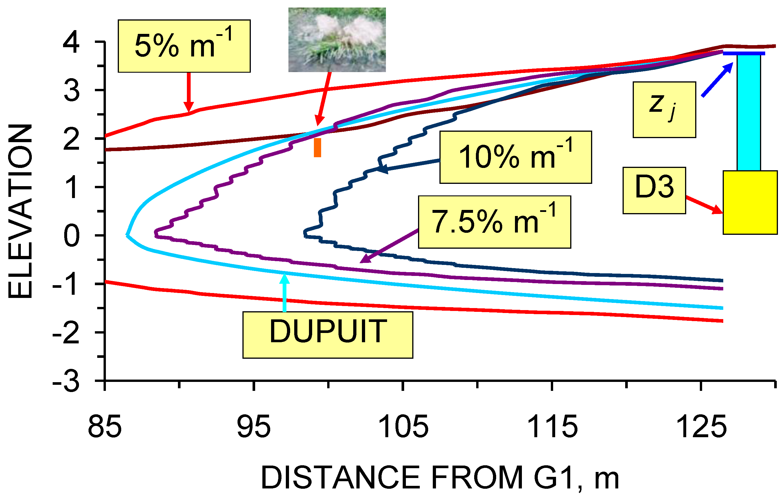
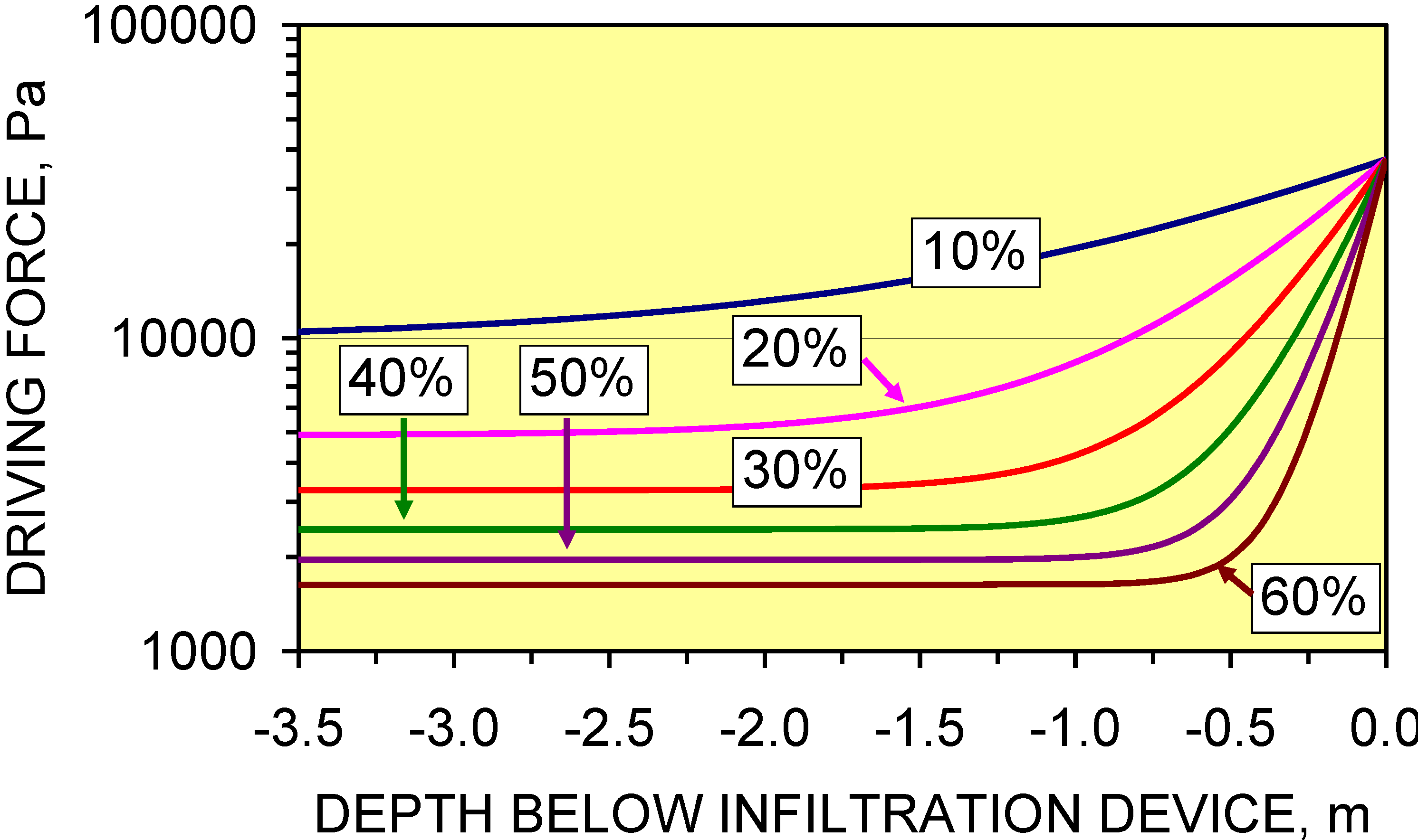
4.4. Impact of Pressure Losses on Groundwater Mound Diameter


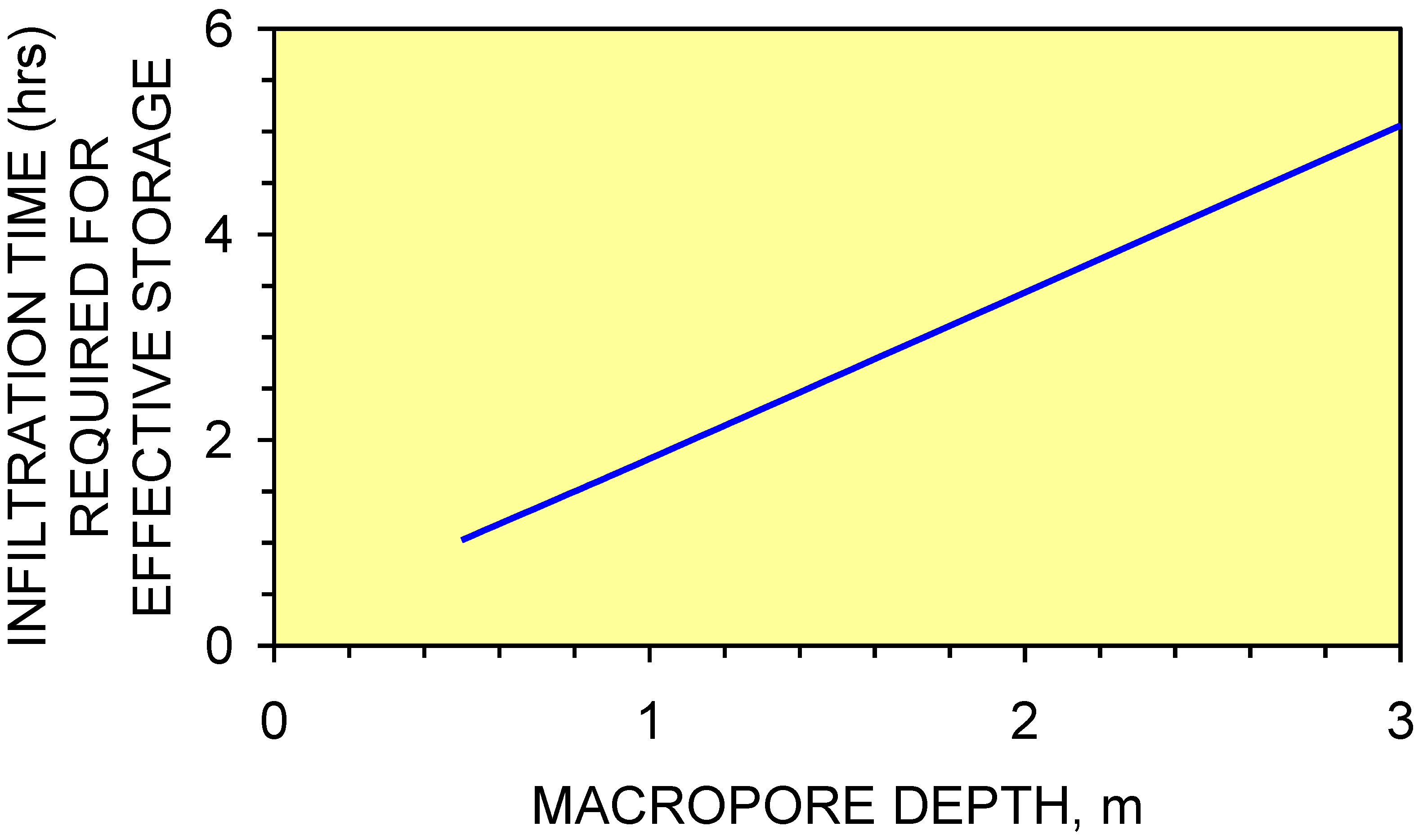
- (i)
- Macropore length (at a specific depth below the AWC) increases with decreasing PL.
- (ii)
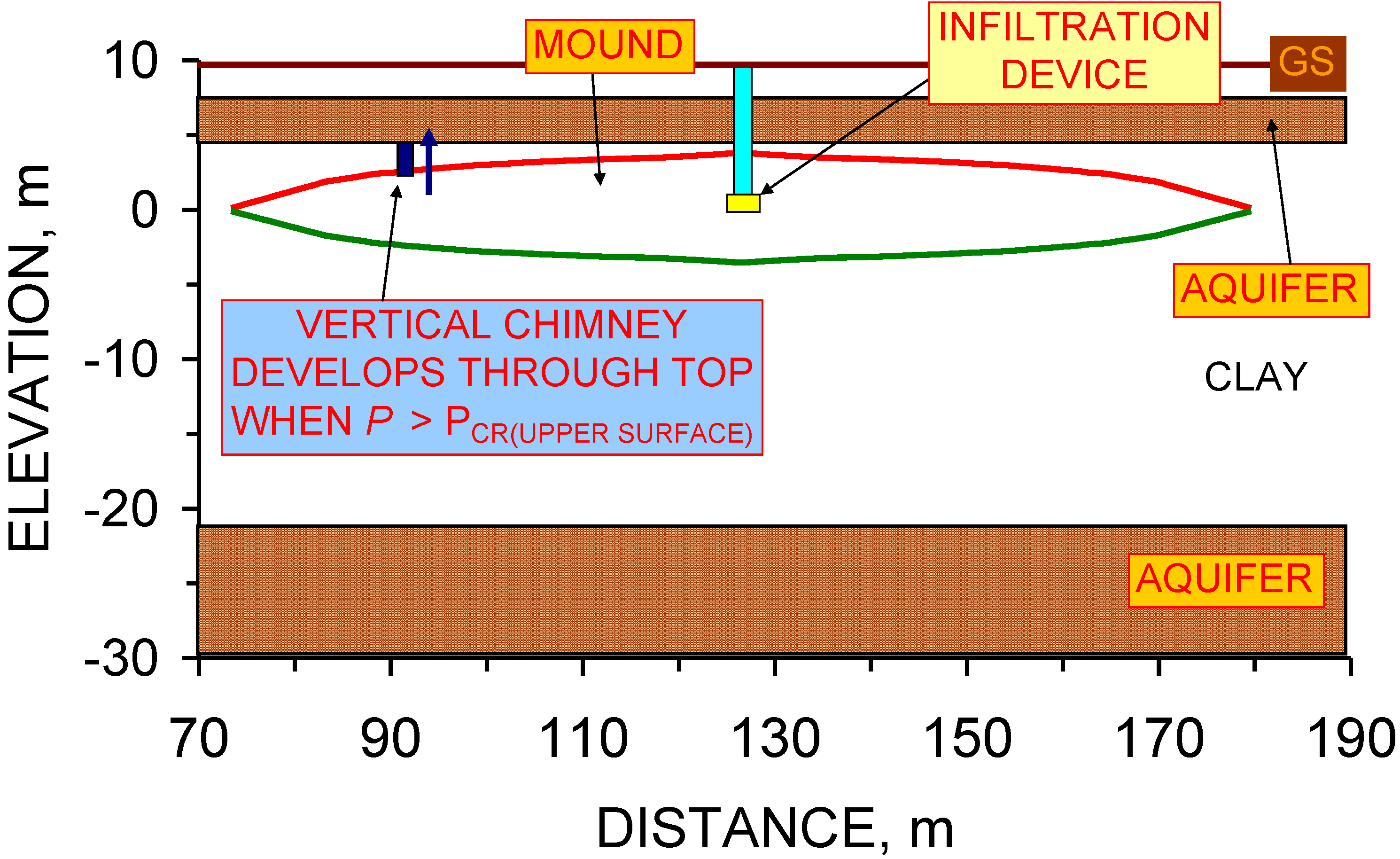
- Shallow macropores at a depth of <1.7 m below the AWC may extend for >40 m from the infiltration device. UK SUDS guidance [7,22,23,29,47] indicates that the groundwater mound associated with an infiltration device in permeable sediment will not extend more than 5 m from the device. This analysis demonstrates that a groundwater mound in impermeable sediment will have a substantially larger (and shallower) radial footprint.
- (iii)
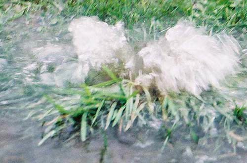
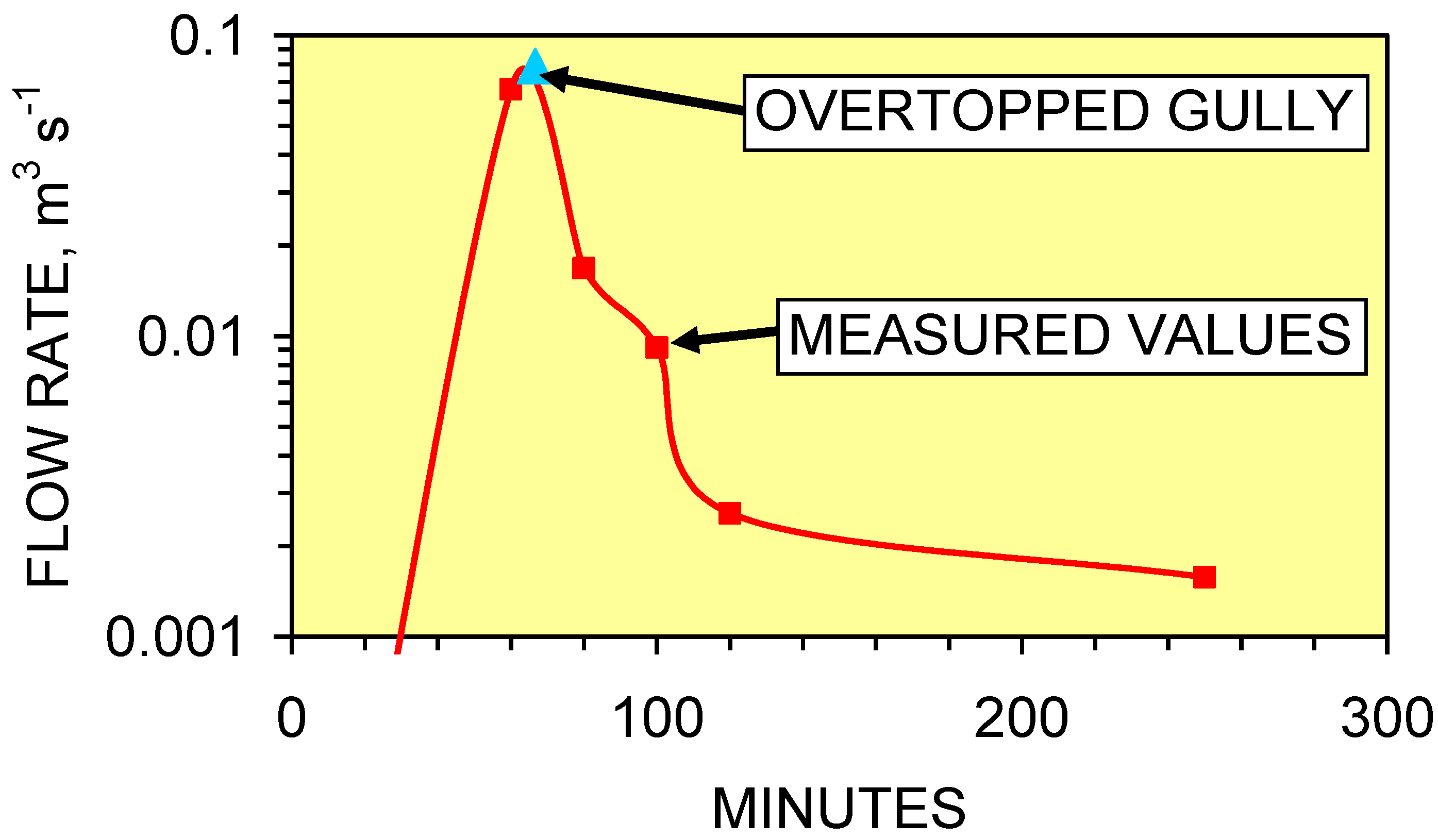
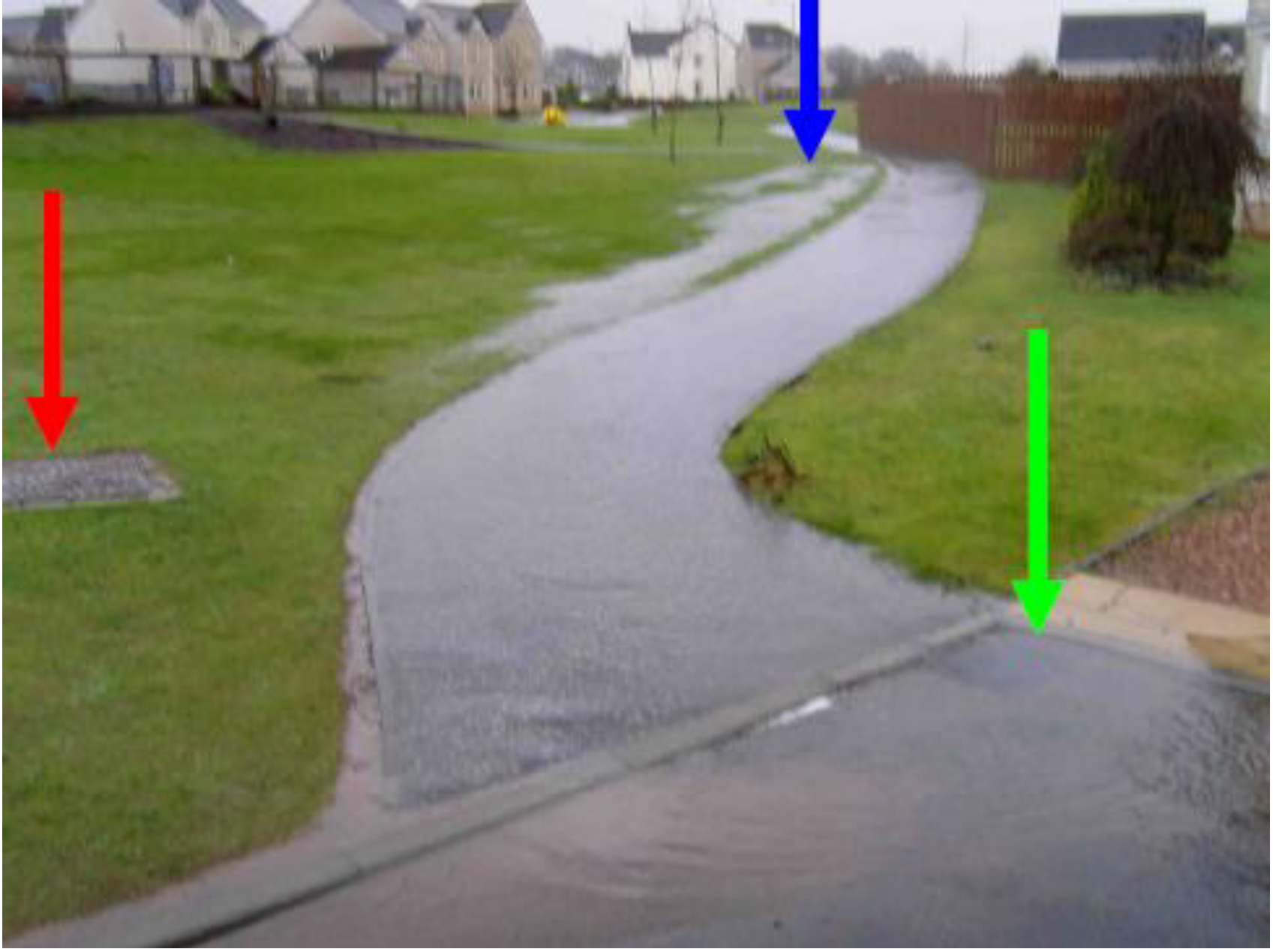
- Infiltration devices placed on sloping sites where the gradient is steeper than 1:50 may experience overland flow due to the groundwater mound rising above the ground surface creating seepage zones.

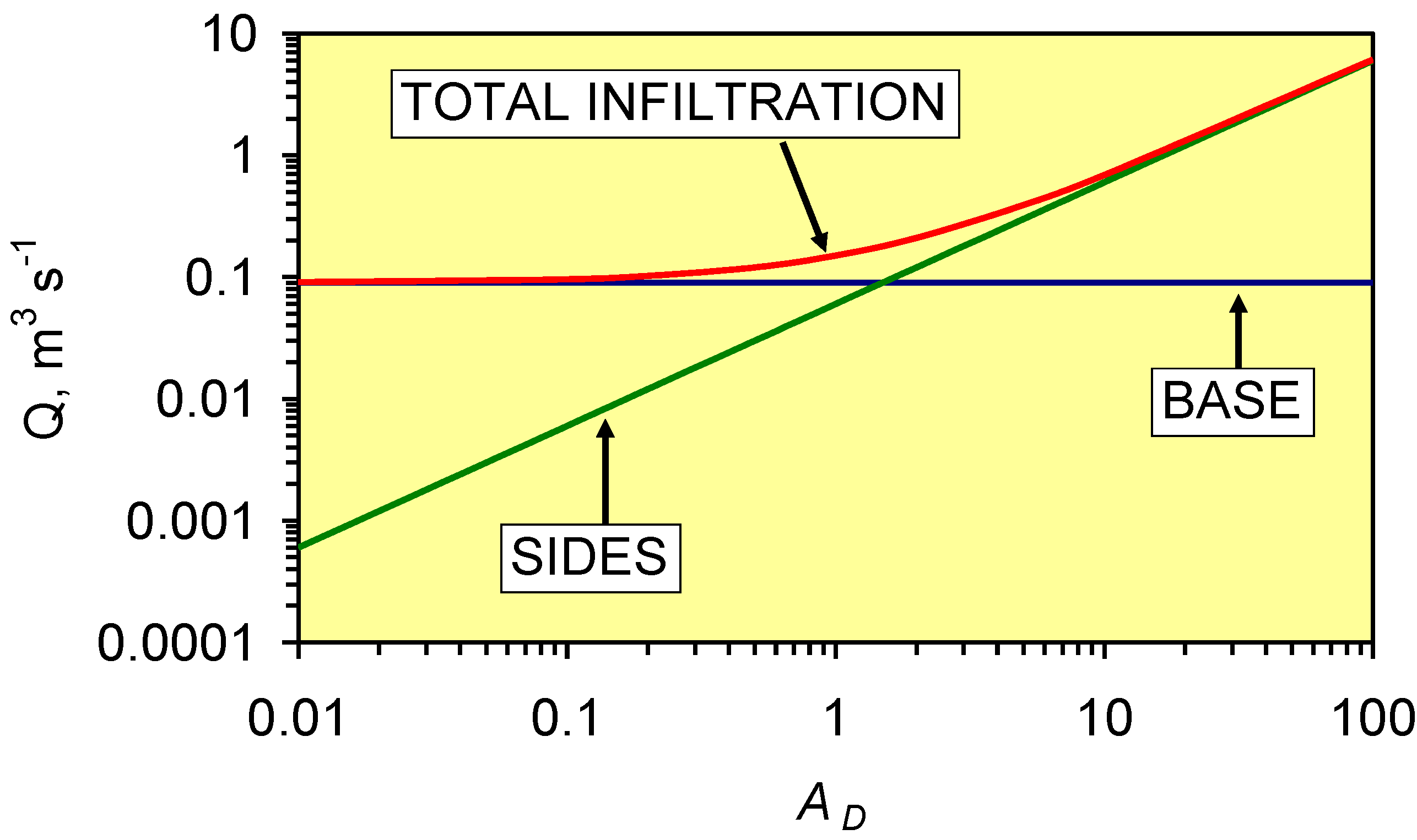
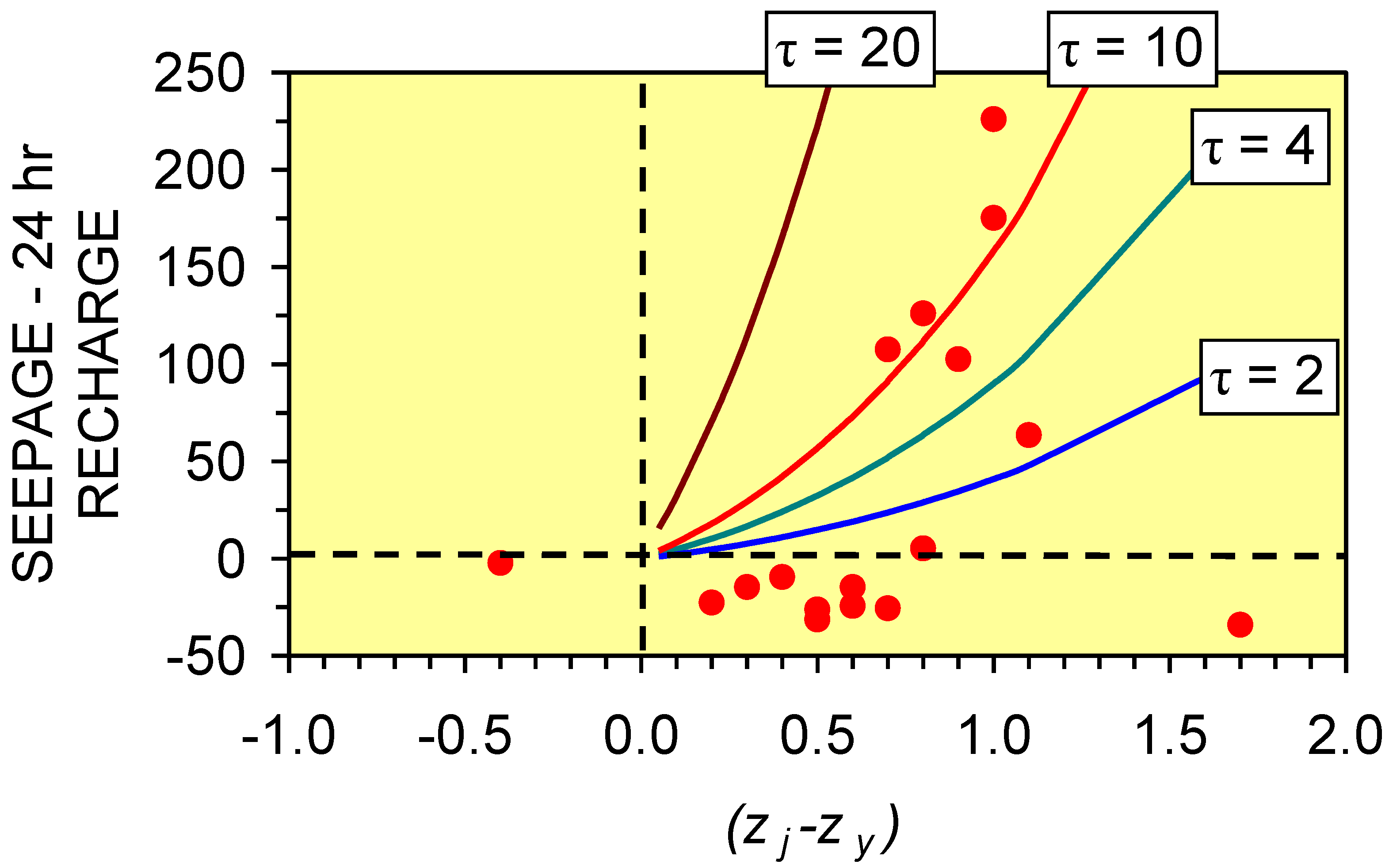
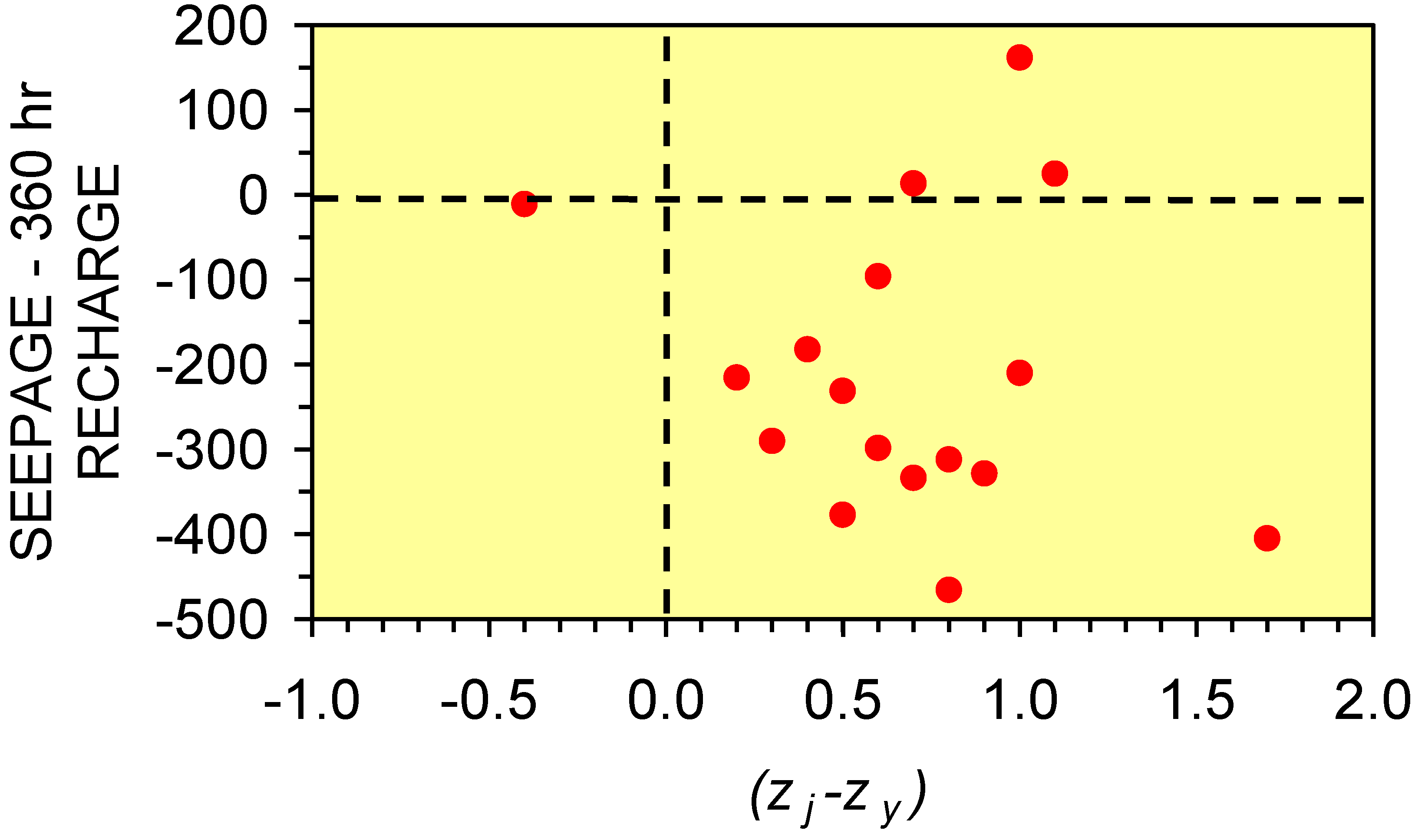
4.5. Seepage Volumes Associated with Groundwater Mounds


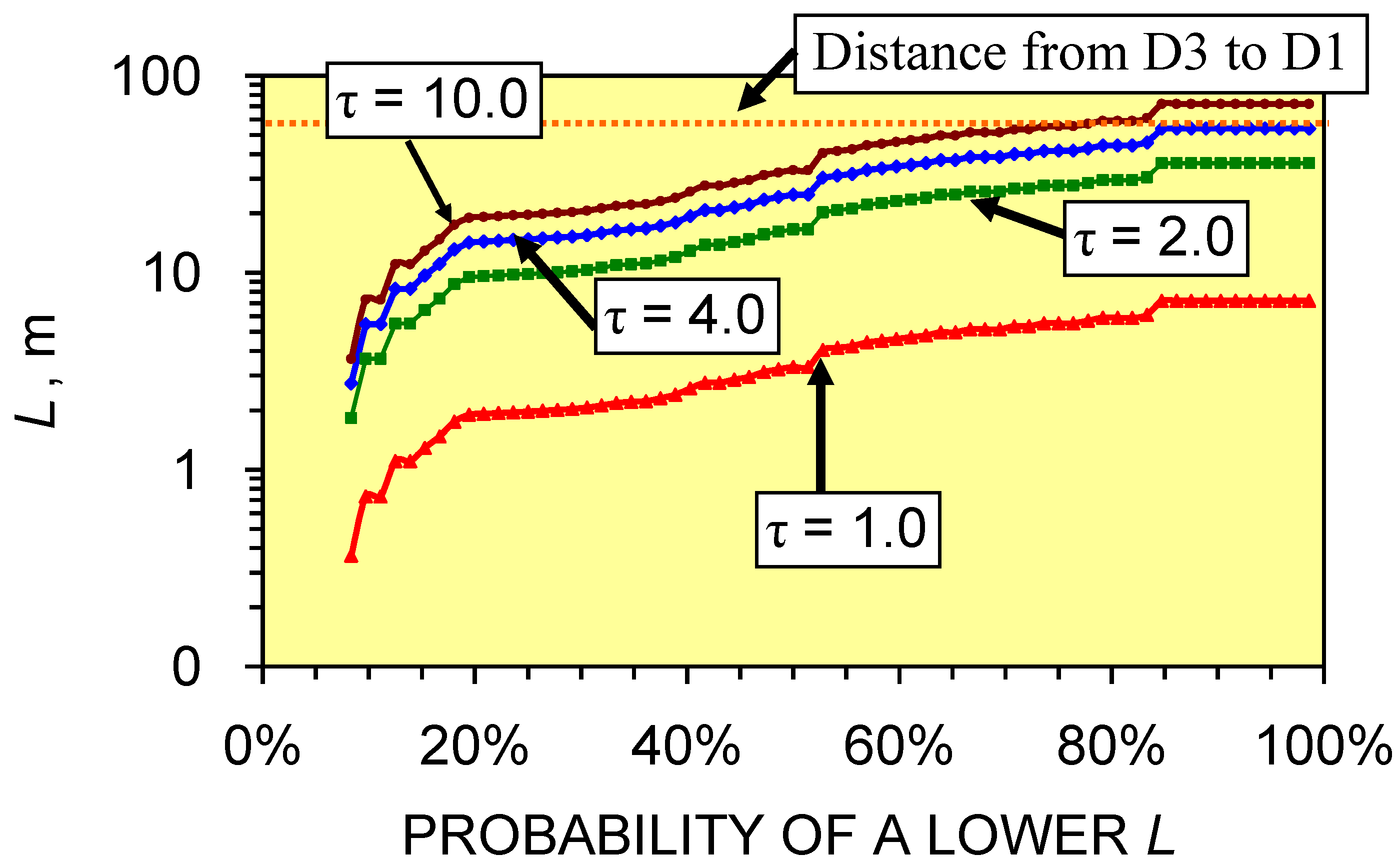
- (i)
- τ,
- (ii)
- the volume of water stored in the groundwater mound prior to the recharge event, and
- (iii)
- recharge volumes over a longer period, rather than a shorter period.
4.5.1. Groundwater mound storage volume
4.5.2. Seepage volumes


5. Modeling a Groundwater Mound for Storage
- (i)
- macropores are used to disperse water from the infiltration device into the surrounding sediments to form a groundwater mound;
- (ii)
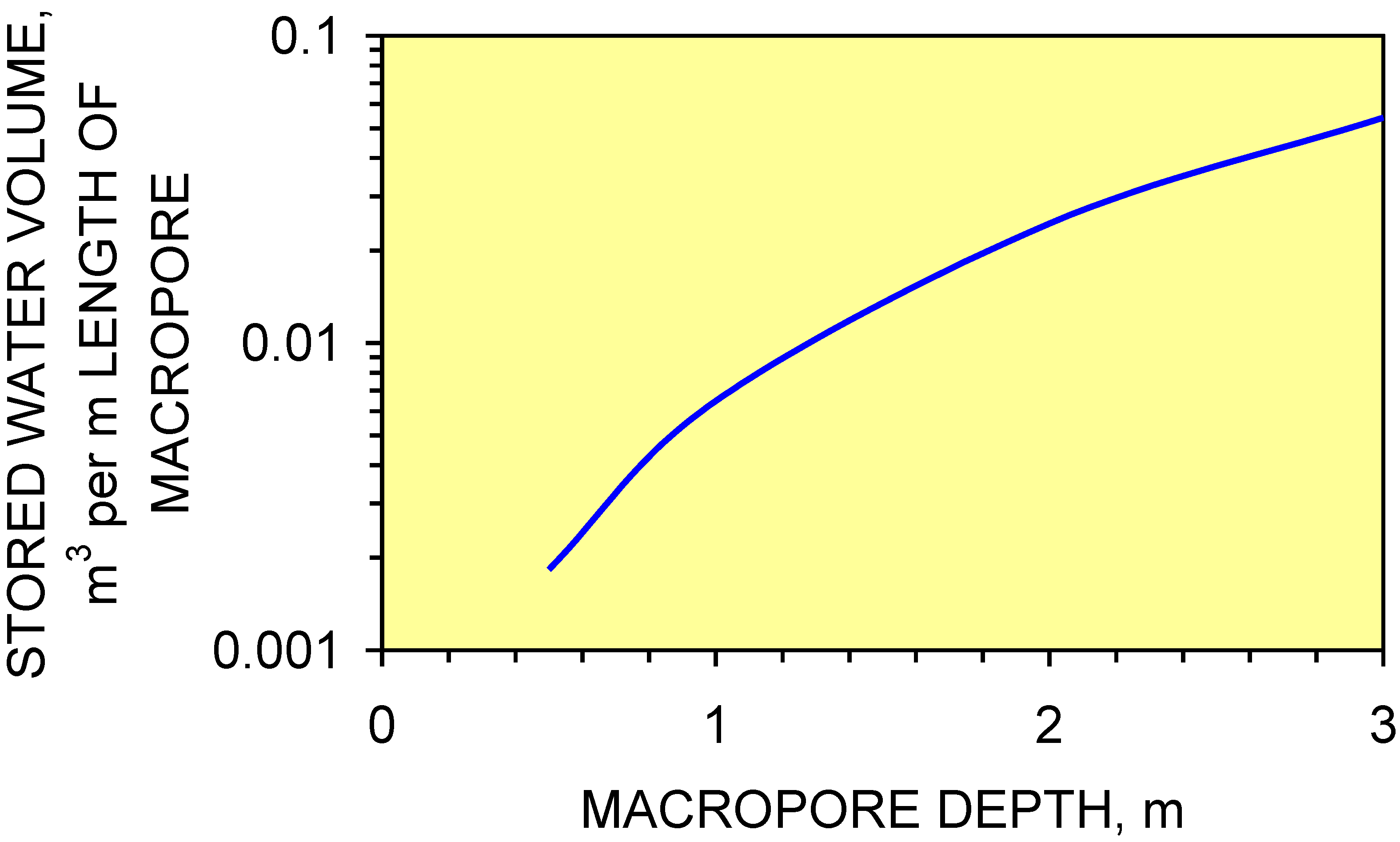
- storage volumes associated with the macropores increase with depth within the mound;
- (iii)
- major conduit or carrier macropores are used to carry large volumes of water within the mound. Where these carrier conduits intersect the ground surface, high volume, high flow rate, discharges occur.
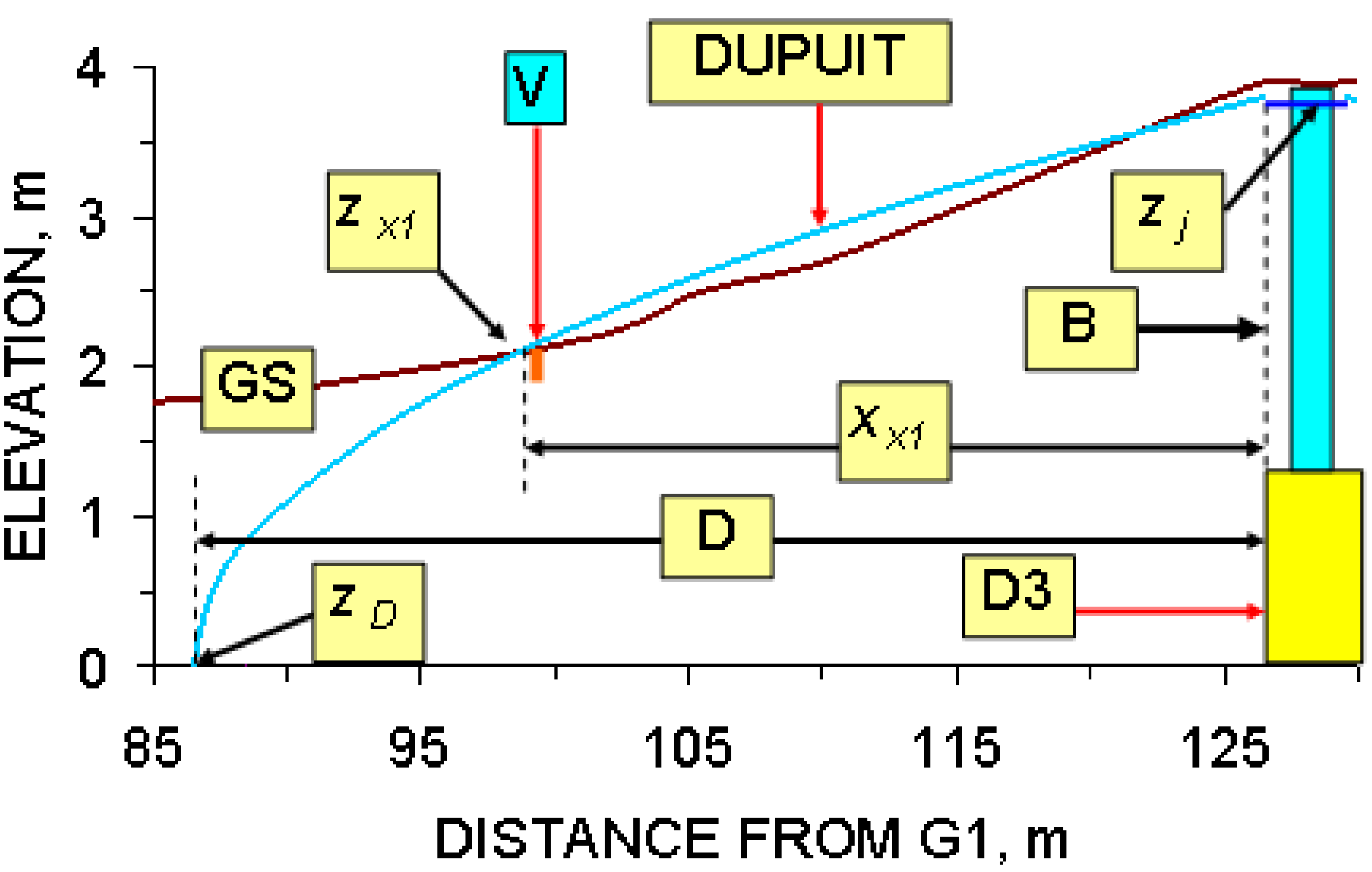
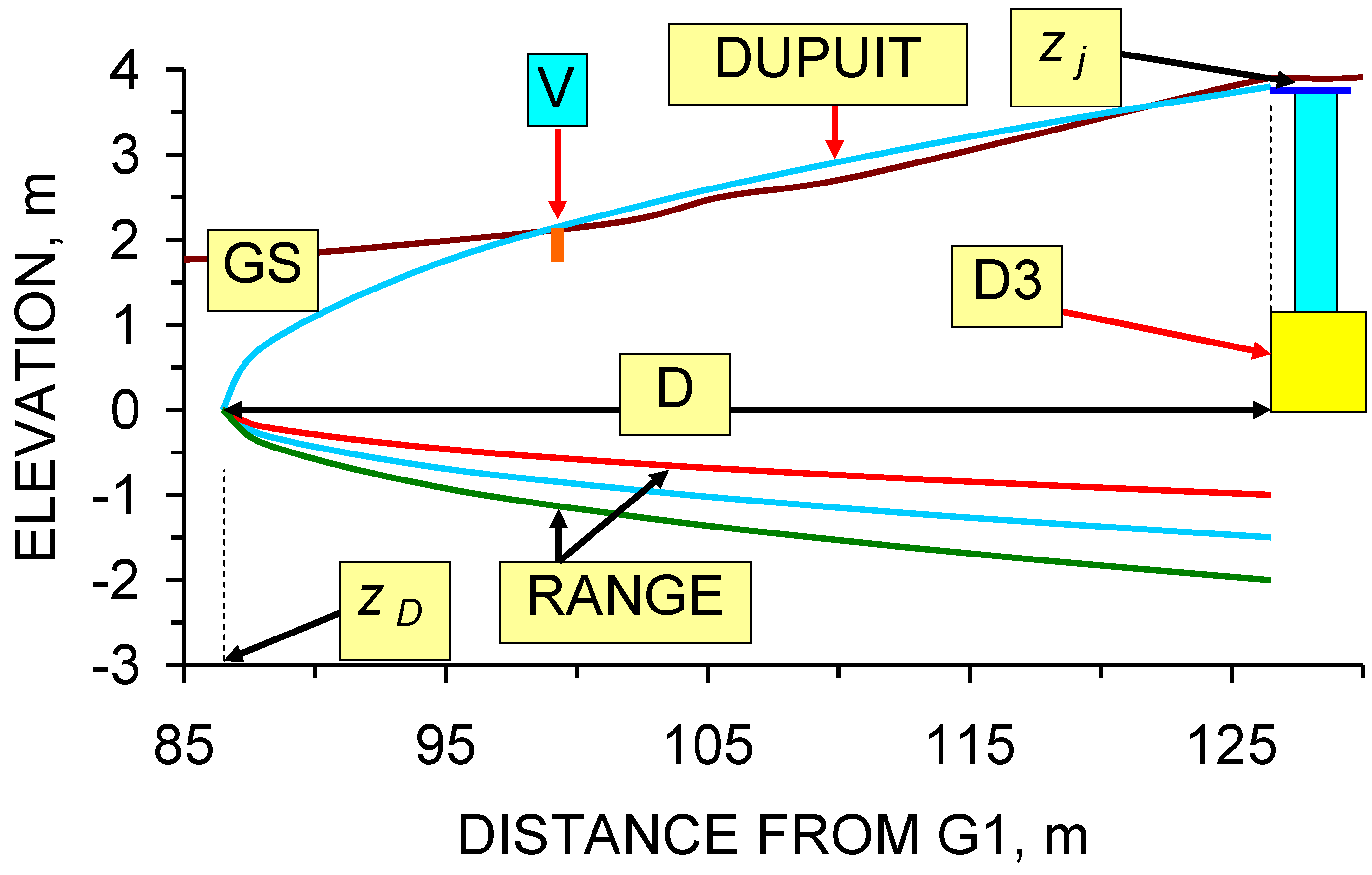
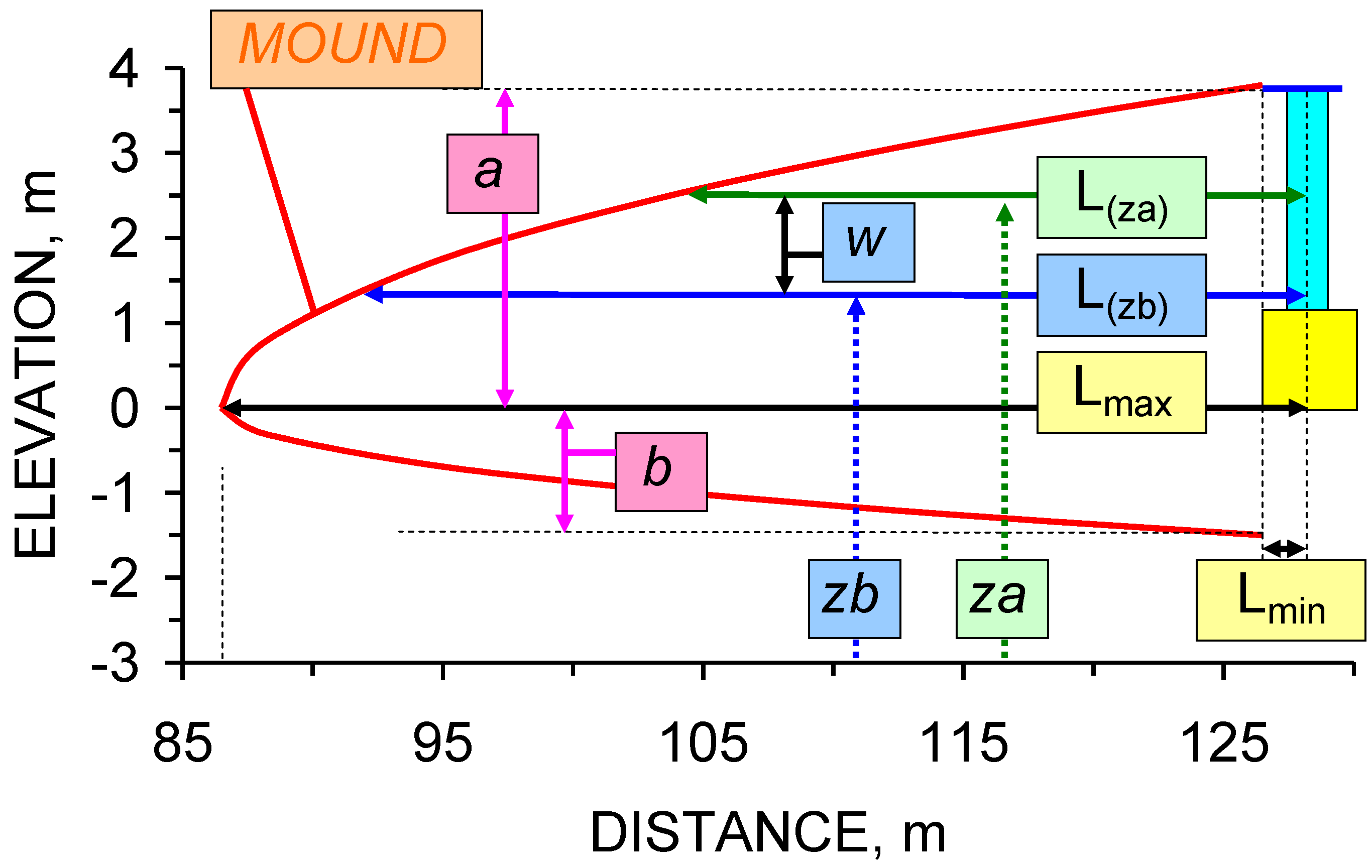
5.1. Upper Surface of the Groundwater Mound: Dupuit Model
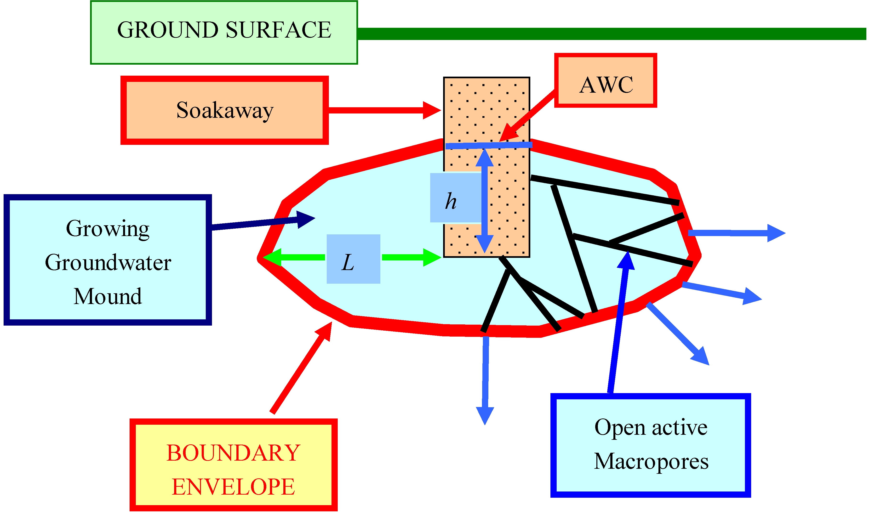
- (i)
- The elevation (m) of the ground surface (GS) relative to the base of the soakaway.
- (ii)
- Distance relative to G1 (m) (or another reference location).
- (iii)
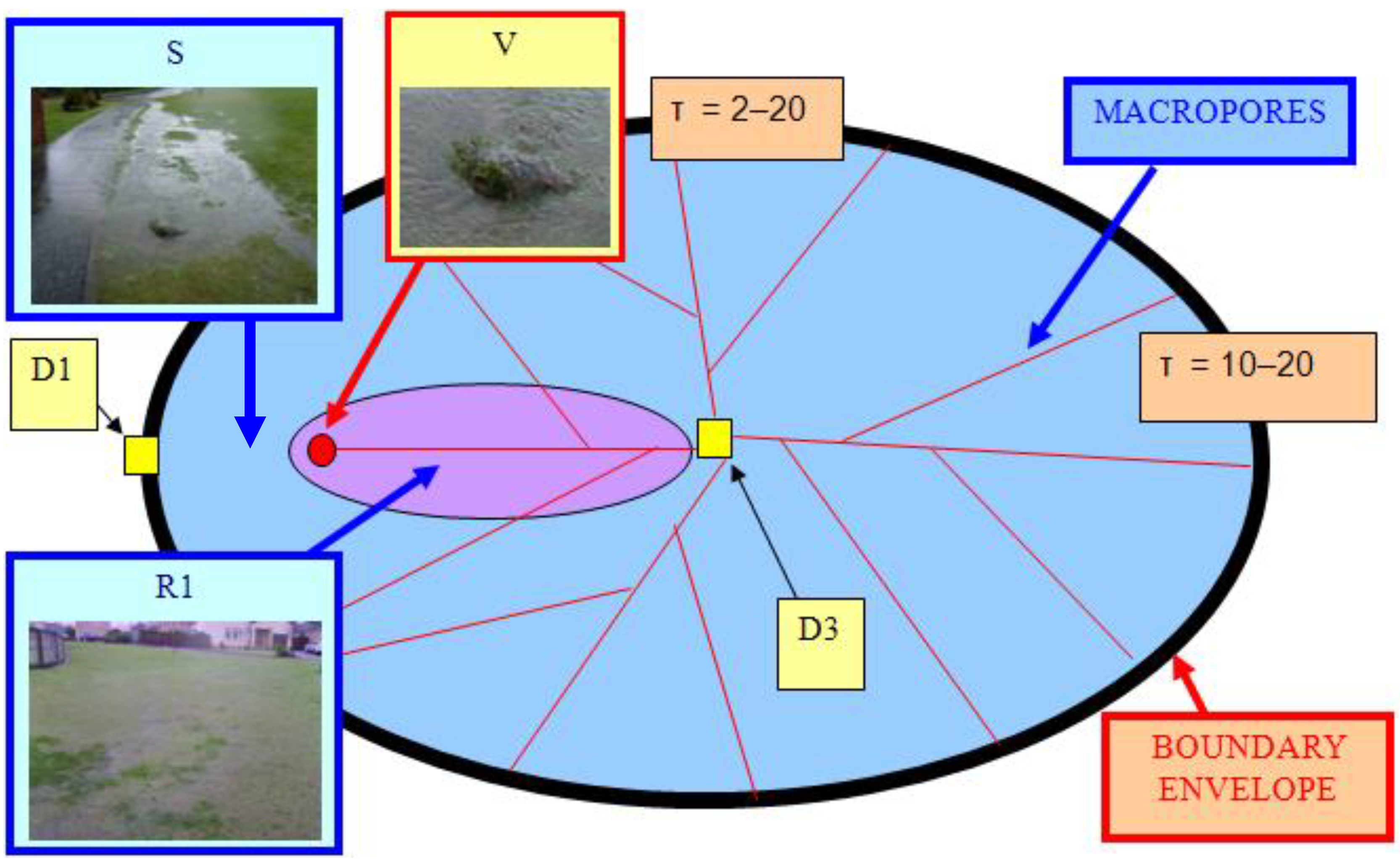
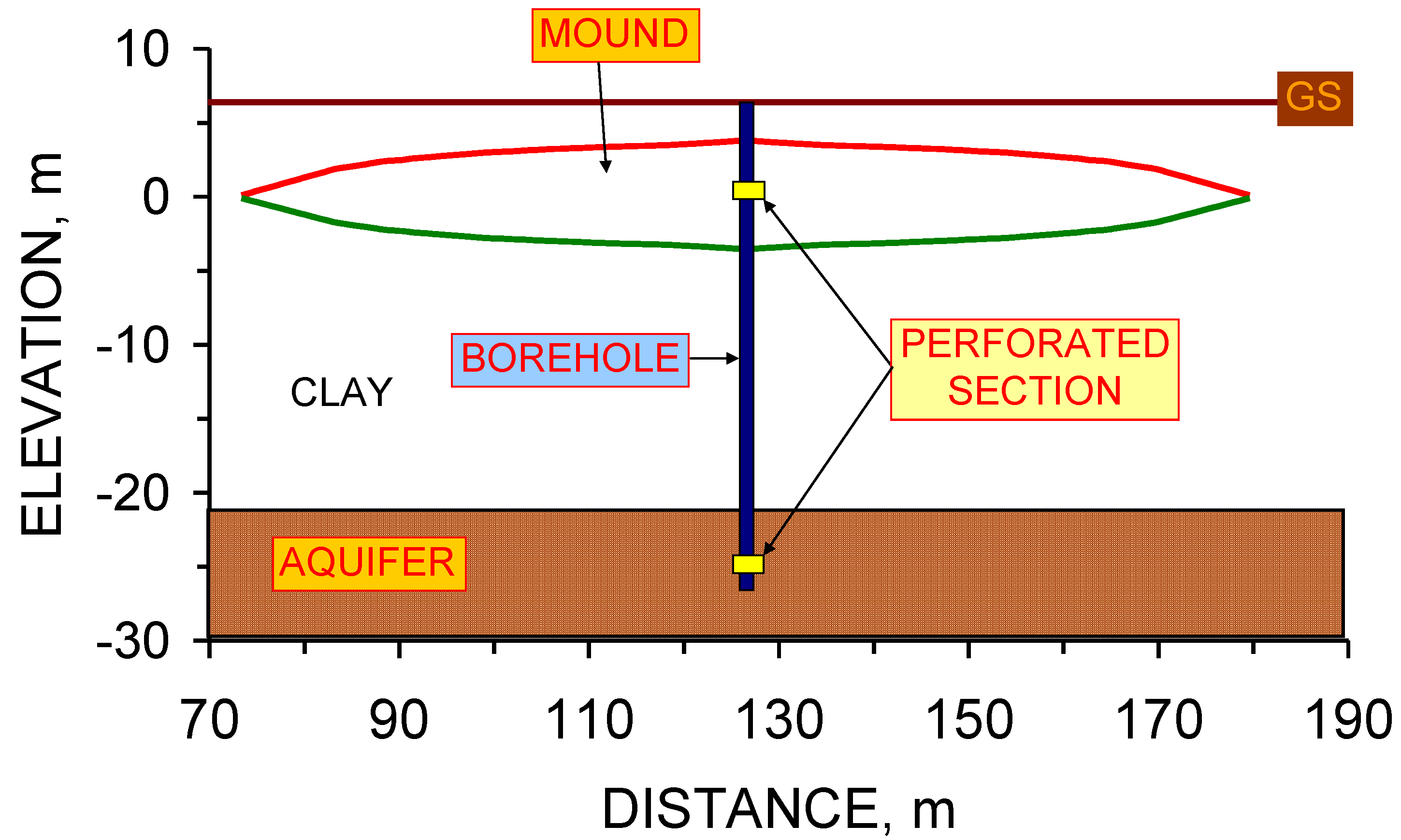
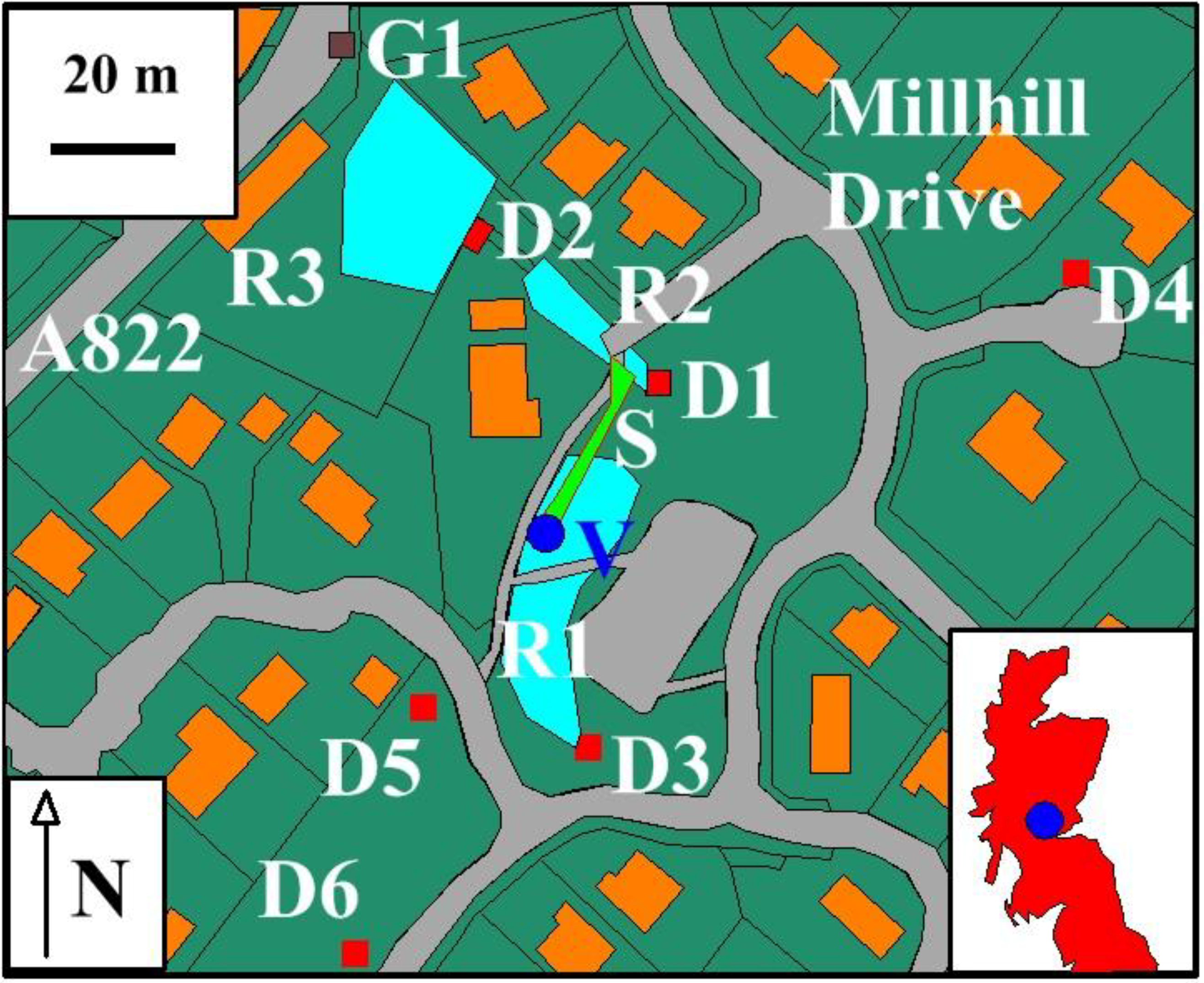
- The location of the soakaway, D3. The D3 soakaway is shown as being 3 m wide and 1.2 m high [1,2]. It consists of a central pre-formed perforated concrete ring, surrounded by coarse gravel. The perforated concrete ring is overlain by a storage chamber made of pre-formed (non-perforated) concrete storage rings [1].
- (iv)
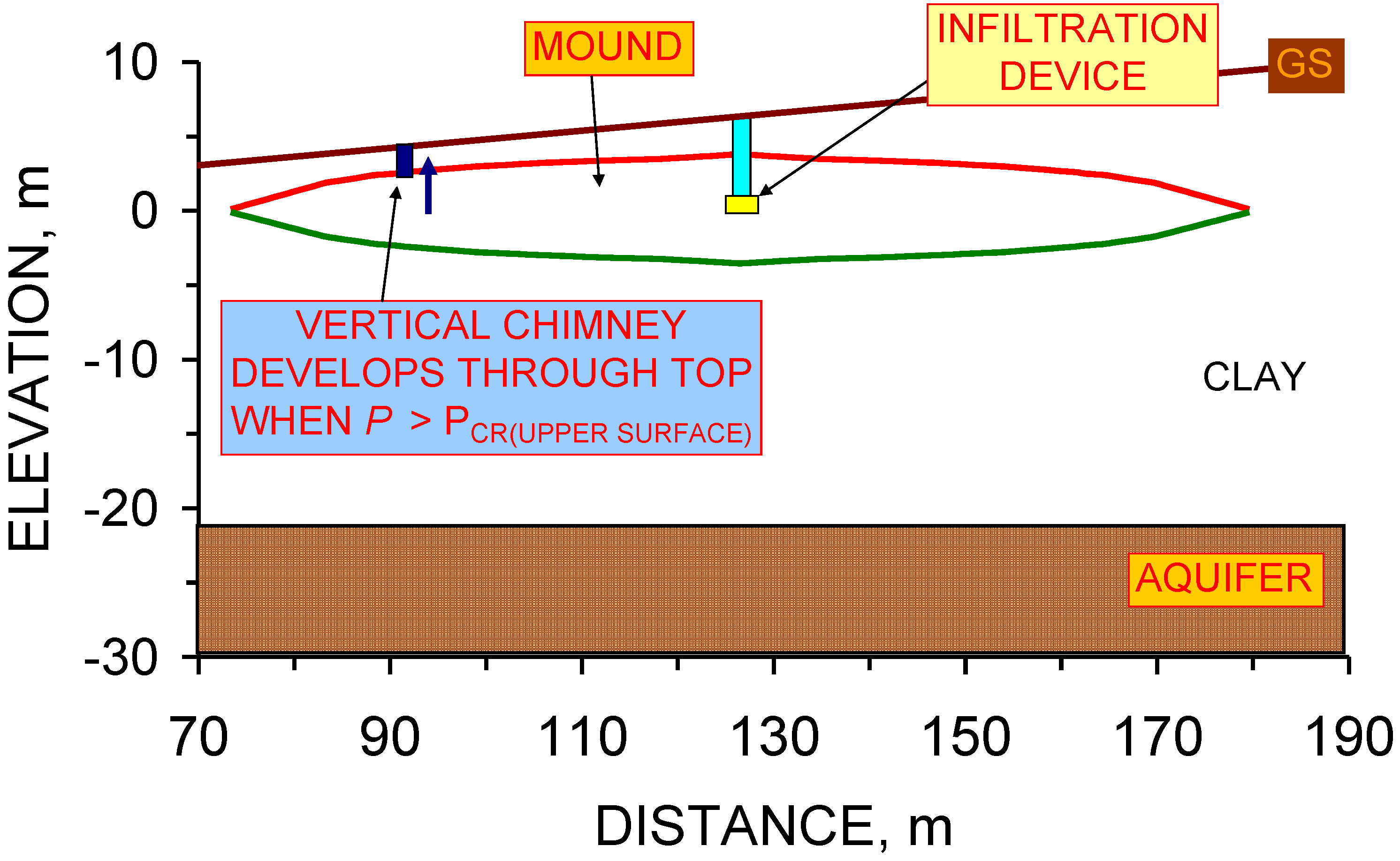
- The groundwater mound can only rise above the ground surface when the air-water contact (zj) in the storage chamber is located above the elevation of the down slope ground surface.
- (v)
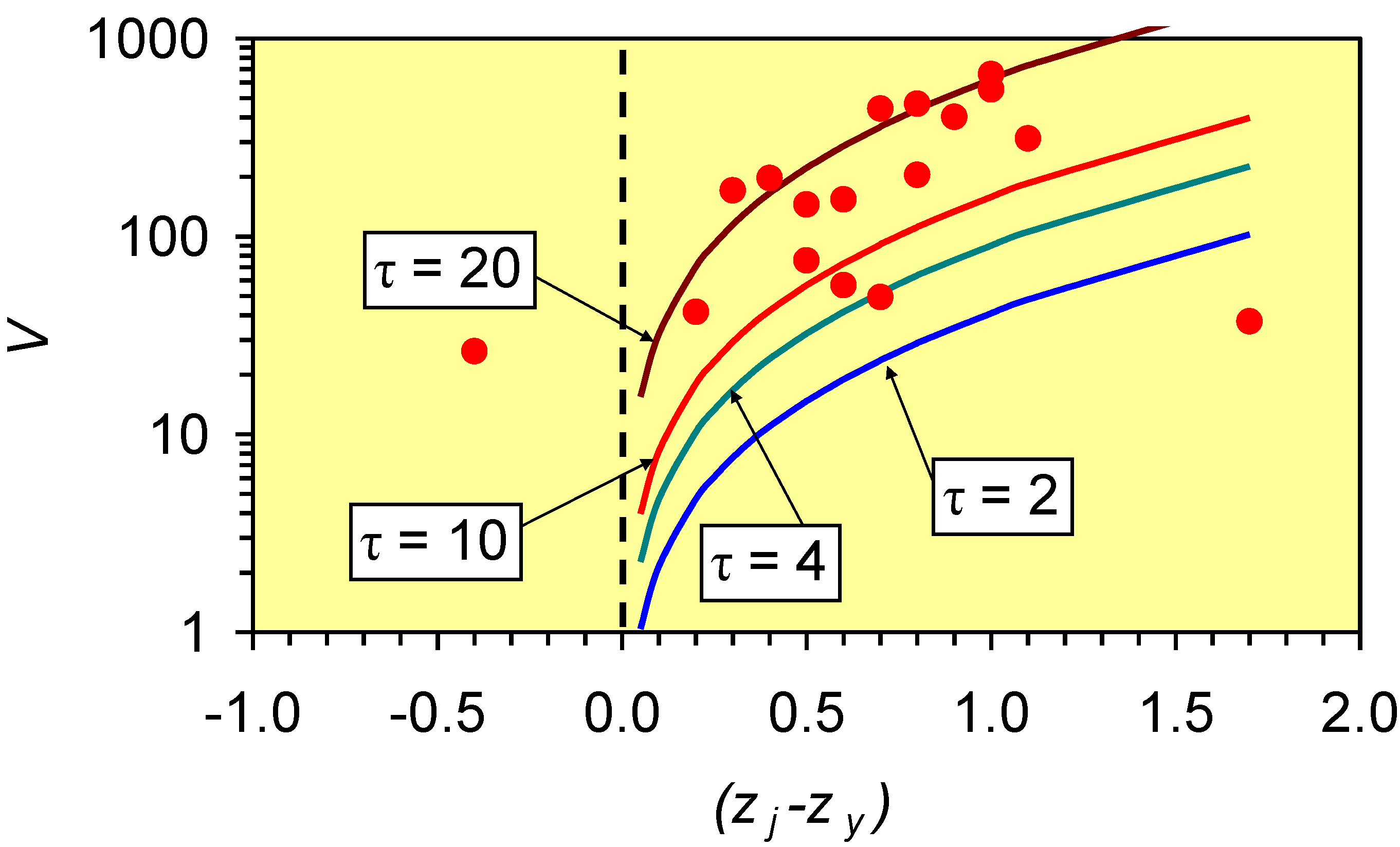
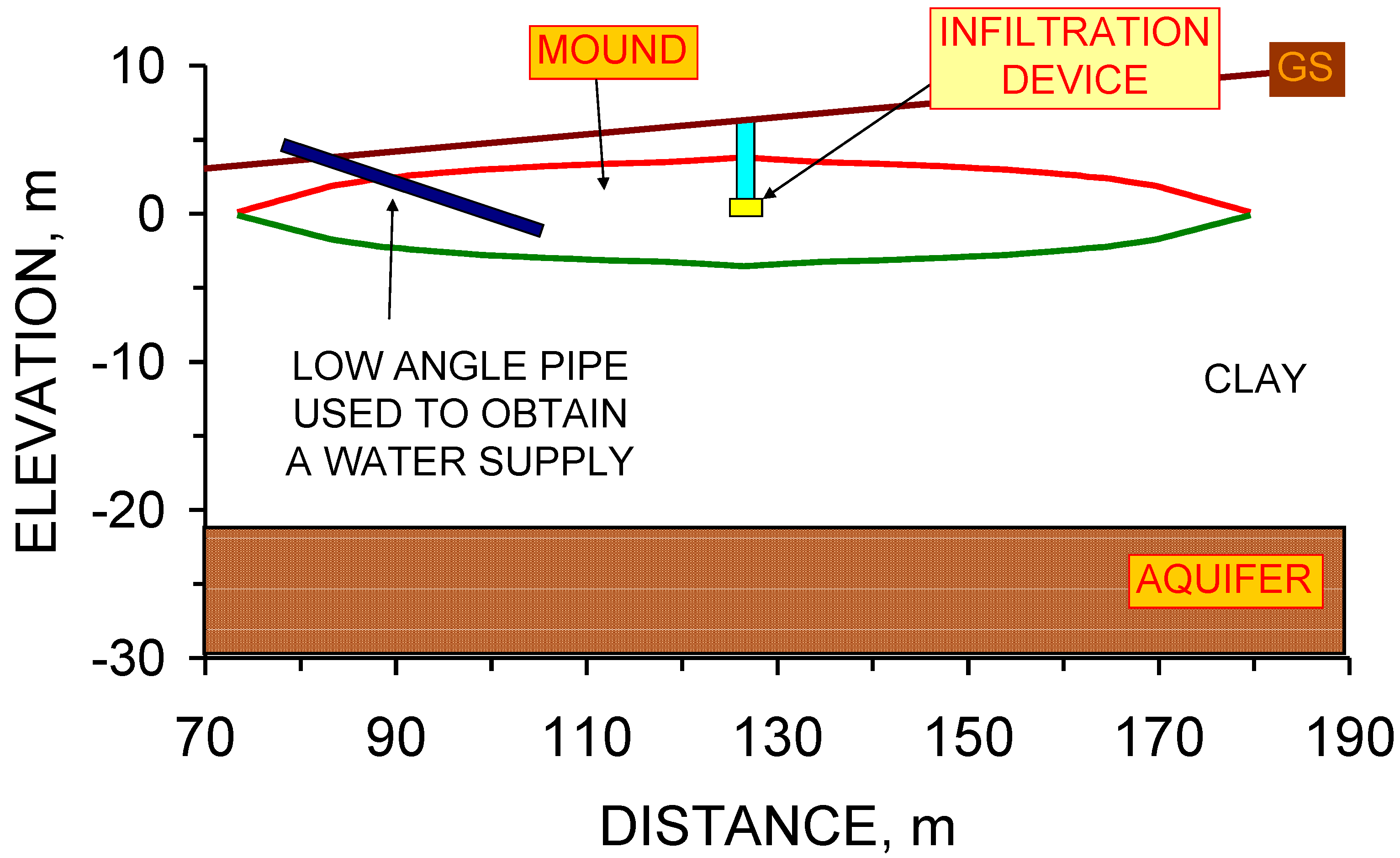
- The location of the vertical macropores (V) marks an intersection point between the groundwater mound and the ground surface (elevation zx1; distance from soakaway, x1).
- (vi)
- Integrating these observations with Equation 15 allows the upper surface of the groundwater mound to be defined as a Dupuit envelope (Figure 61).
- (vii)

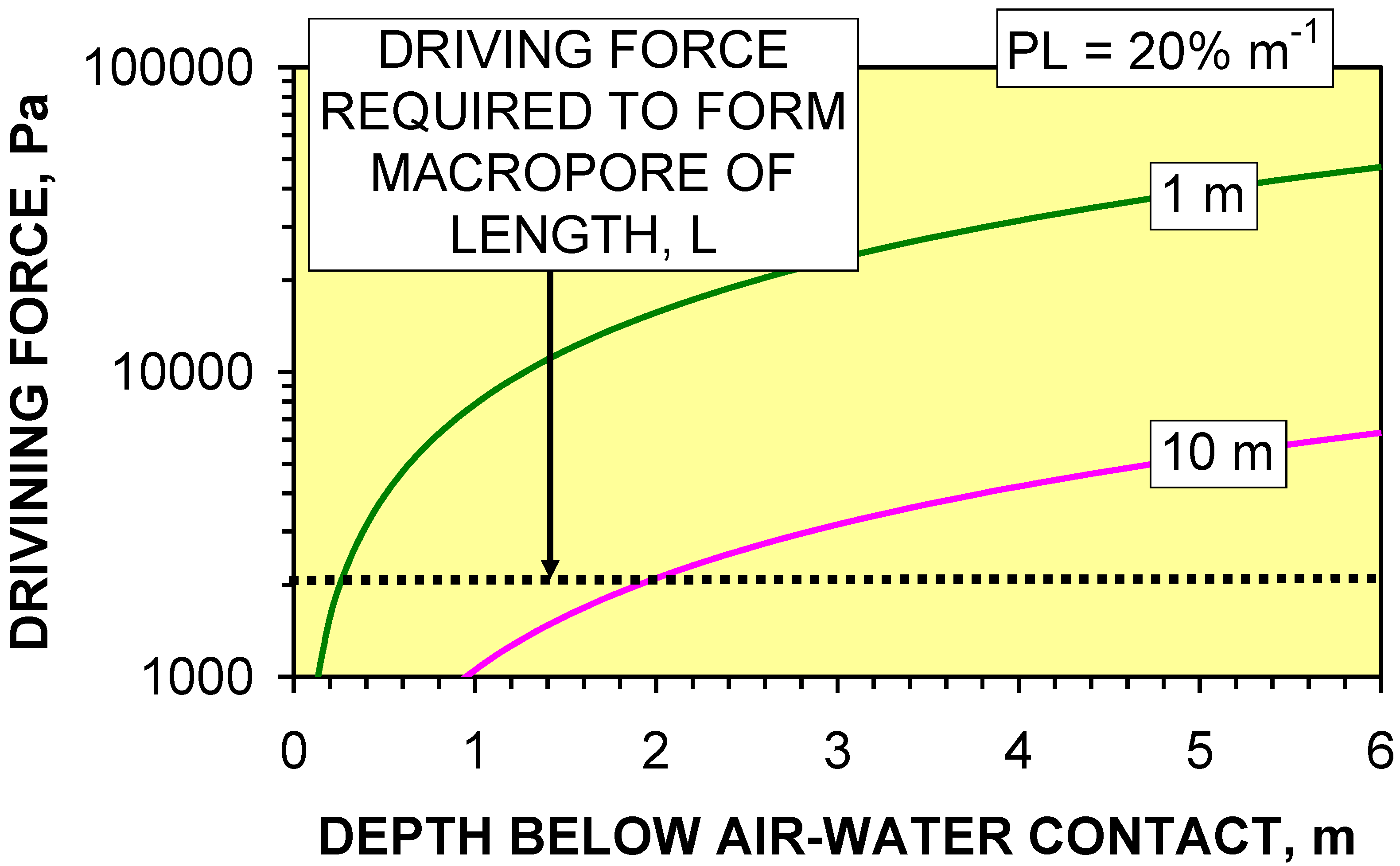
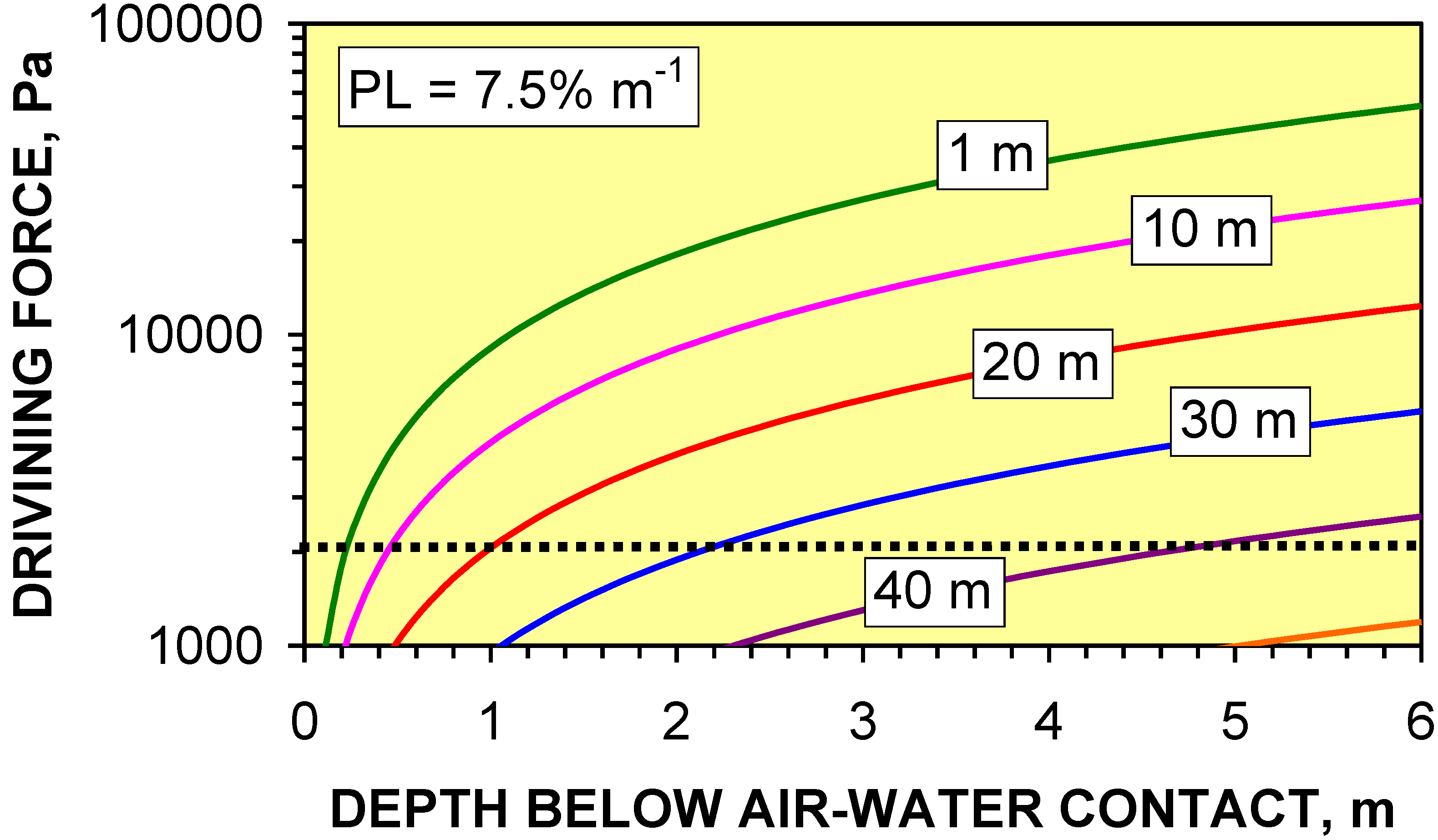
5.2. Upper Surface of the Groundwater Mound: Macropore Propagation Model
- (i)
- the macropore propagation rate (m s–1 Pa–1),
- (ii)
- driving force (Pa) exerted by the infiltration device,
- (iii)
- the critical driving force (Pa) required to initiate macropore propagation, and
- (iv)
- pressure losses (Pa) within the macropore network as a function of distance from the infiltration device (Figure 50).

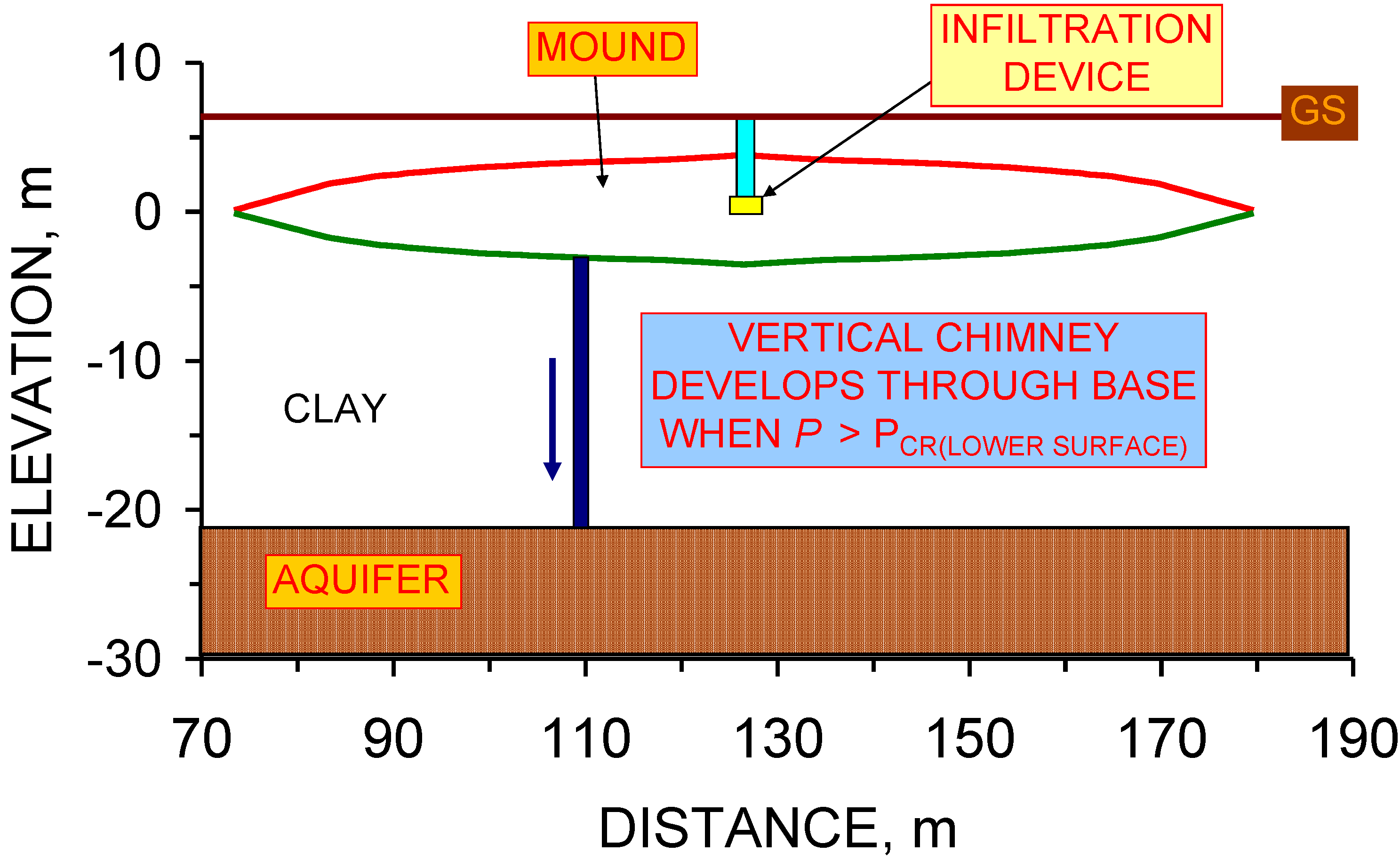
5.3. Lower Surface of the Groundwater Mound: Dupuit Model


5.4. Macropore Analysis of the Lower Surface of the Groundwater Mound

5.5. 3D Mound Volume and Assessment of Potential Resource


5.6. Net Storage Volume

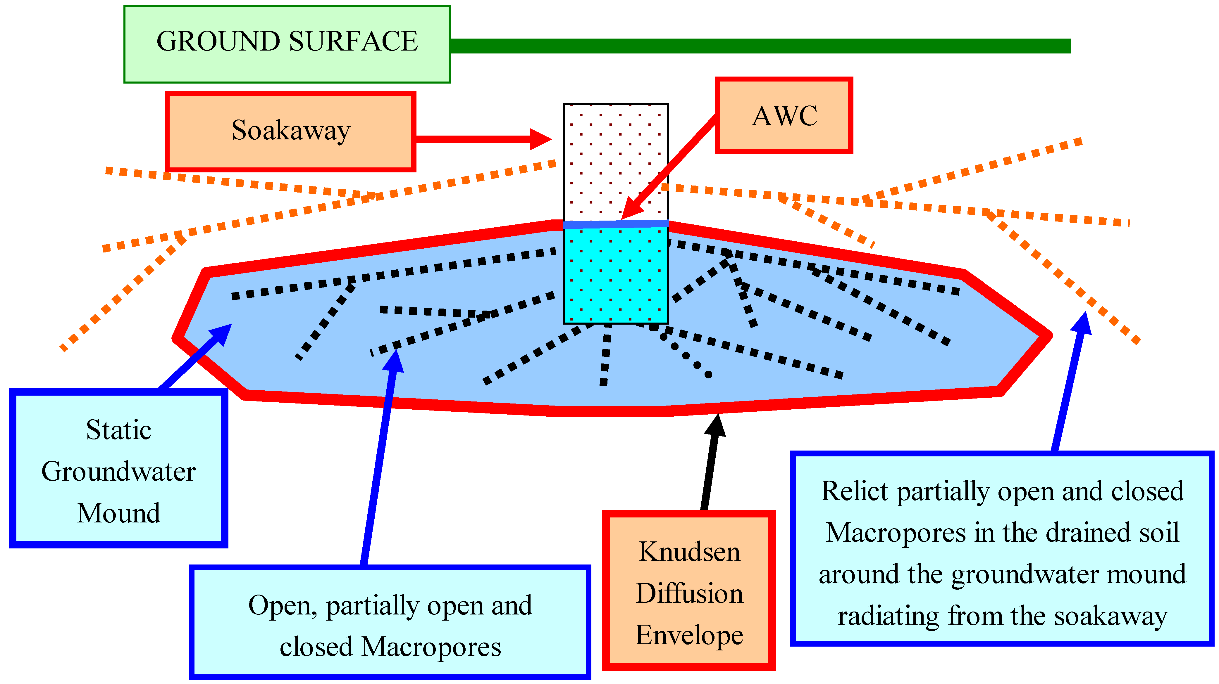
- (i)
- Knudsen diffusion within the sediment matrix,
- (ii)
- macropores extending the groundwater mound into down slope (or adjacent) groundwater mounds,
- (iii)
- fractures allowing infiltration into deeper horizons,
- (iv)
- overland flow when the groundwater mound rises above the ground surface.
5.6.1. Changes in storage capacity with time


5.7. Potential Resource
6. Extraction of Water from a Groundwater Mound


Water Quality
7. Comparison of Observed Results with a Traditional Groundwater Mound Model
7.1. Expected Groundwater Mound Behavior: Arid Environment
7.2. Expected Groundwater Mound Behavior: Modeling
- (i)
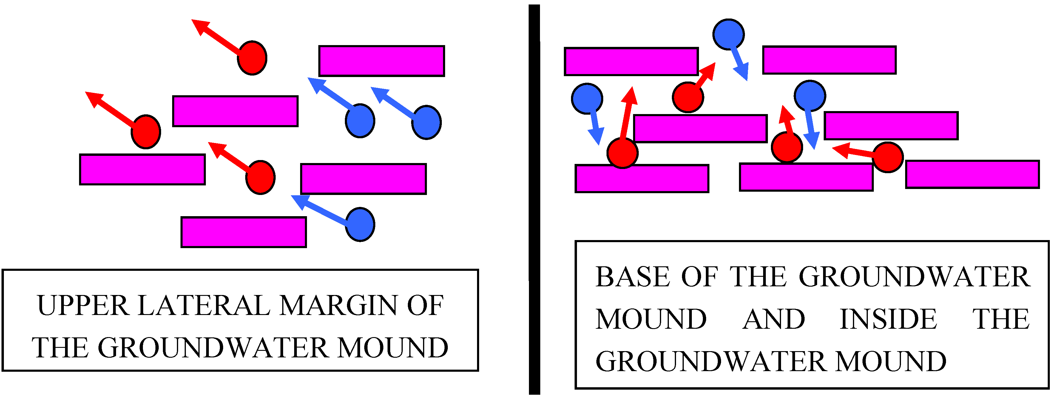
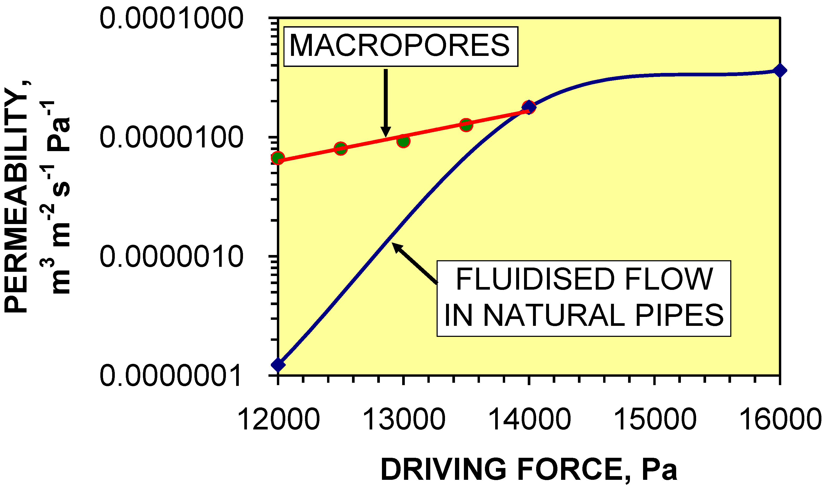
- interactions with the regional water table are not required to produce an effectively static, highly anisotropic, large, perched, groundwater mound in a clayey soil. The mound descends towards the regional water table at a rate dictated by the Knudsen Diffusion permeability of the mound’s boundary layer (e.g., 10–14 m3 m–2 s–1 Pa–1). In the Greenloaning example, a groundwater mound containing a 5 m water column would descend at a maximum rate of <0.16 m yr–1 toward the regional water table. The higher permeability assumptions (relating to the descending wetting front) in the conventional modeling analyses (e.g., 10–9 to 10–13 m3 m–2 s–1 Pa–1) result in a groundwater mound descent of >3.2 m yr–1. The difference in vertical descent rates between the conventional model and Greenloaning observations can be attributed to the observed development of a boundary layer for the groundwater mound, (which is dominated by Knudsen Diffusion (e.g., Figure 17)) and the observed increasing pressure losses within the groundwater mound towards its boundary (e.g., Figure 17 and Figure 18).
- (ii)
- the static groundwater mound will have a very high internal permeability due to the development of macropores and natural pipes (e.g., Figure 16 and Figure 17). This observation allows the static groundwater mound (within a clayey sequence) to act as a very high permeability reservoir. The conventional groundwater mound model assumes a uniform low permeability within the groundwater mound. The conventional model does not recognize the presence of macropores and natural pipes within the mound.
8. Conclusions
Acknowledgements
Appendix 1
A.1. Sustainable Urban Drainage Systems
A.2. Location Map and Details of the Greenloaning Study Area

References
- Antia, D.D.J. Prediction of overland flow and seepage zones associated with the interaction of multiple Infiltration Devices (Cascading Infiltration Devices). Hydrol. Process. 2008, 22, 2595–2614. [Google Scholar] [CrossRef]
- Antia, D.D.J. Interacting infiltration devices (field analysis, experimental observation and numerical modeling): Prediction of seepage (overland flow) locations, mechanisms and volumes—Implications for SUDS, groundwater raising projects and carbon sequestration projects. In Hydraulic Engineering: Structural Applications, Numerical Modeling and Environmental Impacts, 1st ed.; Hirsch, G., Kappel, B., Eds.; Nova Science Publishers: Hauppauge, NY, USA, 2010. [Google Scholar]
- Antia, D.D.J. Oil polymerisation and fluid expulsion from low temperature, low maturity, over pressured sediments. J. Petrol. Geol. 2008, 31, 263–282. [Google Scholar] [CrossRef]
- Antia, D.D.J. Low temperature oil polymerisation and hydrocarbon expulsion from continental shelf and continental slope sediments. Indian J. Petrol. Geol. 2009, 16, 1–30. [Google Scholar]
- Vaughan, P.R. Observations on the behaviour of clay fill containing occluded air bubbles. Geotechnique 2003, 53, 265–272. [Google Scholar] [CrossRef]
- Smoltczyk, V. Geotechnical Engineering Handbook: Fundamentals; Wiley: Chichester, UK, 2002; Volume 1. [Google Scholar]
- Wilson, S.; Bray, R.; Cooper, P. Sustainable Drainage Systems: Hydraulic, Structural and Water Quality Advice, CIRIA Report No. C609; CIRIA: London, UK, 2004. [Google Scholar]
- Bowers, G.L. Detecting high overpressure. Lead. Ed. 2002, 21, 174–177. [Google Scholar] [CrossRef]
- Wolf, L.W.; Lee, M.-K.; Browning, S.; Tuttle, M.P. Numerical analysis of overpressure development in the New Madrid Seismic Zone. Bull. Seism. Soc. Am. 2005, 95, 135–144. [Google Scholar] [CrossRef]
- Antia, D.D.J. Polymerisation Theory–Formation of hydrocarbons in sedimentary strata (hydrates, clays, sandstones, carbonates, evaporites, volcanoclastics) from CH4 and CO2: Part I, Polymerisation concept, kinetics, sources of hydrogen and redox environment. Indian J. Petrol. Geol. 2009, 17(1), 49–86. [Google Scholar]
- Antia, D.D.J. Polymerisation Theory–Formation of hydrocarbons in sedimentary strata (hydrates, clays, sandstones, carbonates, evaporites, volcanoclastics) from CH4 and CO2: Part III: Hydrocarbon expulsion from the hydrodynamic flow regimes contained within a generating pressure mound. Indian J. Petrol. Geol. 2009, 18, 1. (in press). [Google Scholar]
- Opseth, T.L.; Ribsen, B.T.; Syrstad, B.; Huse, A.; Bolstad, L.; Saasen, A. Curing shallow water flow in a North Sea Exploration well exposed to shallow gas. SPE Pap. 2009, SPE 124607. [Google Scholar]
- Highways Agency. Design Manual for Roads and Bridges, Volume 4: Geotechnics and Drainage; Section 2: Drainage: HA 37/97. Hydraulic Design of Road Edge Surface Water Channels; Stationary Office Ltd.: London, UK, 1997. [Google Scholar]
- Brutsaert, W. Hydrology an Introduction; Cambridge University Press: Cambridge, UK, 2005. [Google Scholar]
- BRE. Soakaway Design, Digest 365; HIS BRE Press: Garston, UK, 1991. [Google Scholar]
- Flood Studies Report in Five Volumes, Volume II, Meteorological Studies; Institute of Hydrology: Wallingford, UK, 1993.
- Bettess, R. Infiltration Drainage–Manual of Good Practice, CIRIA Report No. C156; CIRIA: London, UK, 1996. [Google Scholar]
- Kim, H. Anisotropic Properties of Compacted Silty Clay. MSc. Thesis, Ohio University, Athens, OH, USA, 1996. [Google Scholar]
- Mulder, M. Basic Principles of Membrane Technology; Kluwer Academic Publishers: Dordrecht, The Netherlands, 1996. [Google Scholar]
- Misstear, B.; Banks, D.; Clark, L. Water Wells and Boreholes; Wiley: Chichester, UK, 2006. [Google Scholar]
- Lide, D.R. CRC Handbook of Chemistry and Physics, 89th ed.; CRC Press: London, UK, 2008. [Google Scholar]
- Martin, P.; Turner, B.; Waddington, K.; Pratt, C.; Campbell, N.; Payne, J.; Reed, B. Sustainable Urban Drainage Systems: Design Manual for Scotland and Northern Ireland, CIRIA Report No. C521; CIRIA: London, UK, 2000. [Google Scholar]
- Martin, P.; Turner, B.; Waddington, K.; Pratt, C.; Campbell, N.; Payne, J.; Reed, B. Sustainable Urban Drainage Systems: Design Manual for England and Wales, CIRIA Report No. C522; CIRIA: London, UK, 2000. [Google Scholar]
- Pratt, C.J. Sustainable drainage: A review of published material on the performance of various SUDS components. Prepared for the Environment Agency. SUDS Science Group /99705.015. 2004. Available online: http://ciria.org/suds/pdf/suds_lit_review_04.pdf (accessed May 2009).
- Campbell, N.S.; D’Arcy, B.; Frost, A.; Novotny, V.; Sansom, A. Diffuse Pollution; IWA Publishing: London, UK, 2005. [Google Scholar]
- Pratt, C.J. Research and development in methods of soakaway design. Water Environ. J. 1996, 10, 47–51. [Google Scholar] [CrossRef]
- Butler, D.; Davis, J. Urban Drainage; Spon Press: London, UK, 2004. [Google Scholar]
- Highways Agency. Design Manual for Roads and Bridges; Volume 4: Geotechnics and Drainage; Section 2: Drainage: Part 8, HA 118/06, Design of soakaways; Stationary Office Ltd.: London, UK, 2006. [Google Scholar]
- Woods Ballard, B.; Kellagher, R.; Martin, P.; Jefferies, C.; Bray, R.; Shaffer, P. The SUDS Manual, CIRIA Report No. C697; CIRIA: London, UK, 2007. [Google Scholar]
- Woods Ballard, B.; Kellagher, R.; Martin, P.; Jefferies, C.; Bray, R.; Shaffer, P. Site Handbook for the Construction of SUDS, CIRIA Report No. C698; CIRIA: London, UK, 2007. [Google Scholar]
- Cipriano, B.H.; Raghaven, S.R.; McGuiggan, P.M. Surface tension and contact angle measurements of a hexadecylimidazolium surfactant adsorbed on a clay surface. Colloids Surf. A 2005, 262, 8–13. [Google Scholar] [CrossRef]
- Schramm, L.L.; Hepler, L.G. Surface and interfacial tensions of aqueous dispersions of charged colloidal (clay) particles. Can. J. Chem. 1994, 72, 1915–1920. [Google Scholar] [CrossRef]
- Motealleh, S.; Bryant, S.L. Quantitative mechanism for permeability reduction by small water saturation in tight-gas sandstones. SPE J. 2009, 14, 252–258. [Google Scholar] [CrossRef]
- Easterbrook, D.J. Glacial sediments. In Sandstone Depositional Environments; Scholle, P.A., Spearing, D., Eds.; American Association of Petroleum Geologists: Tulsa, OK, USA, 1982; pp. 1–10. [Google Scholar]
- Trenter, N.A. Engineering in Glacial Tills, CIRIA Report C504; CIRIA: London, UK.
- Murray, H.H. Applied Clay Mineralogy: Occurrences, Processing and Applications for Kaolins, Bentonites, Palygorskitesepiolite and Common Clays; Elsevier: Amsterdam, The Netherlands, 2007. [Google Scholar]
- Zhu, H.Y.; Yamanaka, S. Molecular recognition of Na-loaded alumina pillared clay. J. Chem. Soc., Faraday Trans. 1997, 93, 477–480. [Google Scholar] [CrossRef]
- Chatterjee, A. Application of localized reactivity index in combination with periodic DFT calculation to rationalise the swelling mechanism of clay type in organic matter. J. Chem. Sci. 2005, 117, 533–539. [Google Scholar] [CrossRef]
- Alcover, J.-F.; Al-Mukhtar, Y.; Qi, M.; Bonnamy, S.; Bergaya, F. Hydromechanical effects on the Na-smectite microtexture. Clay Miner. 2000, 35, 525–536. [Google Scholar] [CrossRef]
- Jena, H.M.; Roy, G.K.; Meikap, B.C. Hydrodynamics of a gas-liquid-solid fluidised bed with hollow cylindrical particles. J. Chem. Eng. Process. 2009, 48, 279–287. [Google Scholar] [CrossRef]
- Benson, C.H.; Daniel, D.E. Influence of clods on the hydraulic conductivity of compacted clay. J. Geotech. Eng. 1990, 116, 1231–1248. [Google Scholar] [CrossRef]
- Keijzer, Th.J.S.; Kleingeld, P.J.; Loch, J.P.G. Chemical osmosis in compacted clayey material and the prediction of water transport. Engrg. Geol. 1999, 53, 151–159. [Google Scholar] [CrossRef]
- Coats, J.S.; Shaw, M.H.; Gallagher, M.J.; Armstrong, M.; Greenwood, P.G.; Chacksfield, B.C.; Williamson, J.P.; Fortey, N.J. Gold in the Ochil Hills. British Geological Survey Technical Report WF/91/1, Mineral Reconnaissance Programme Report 116; NERC: London, UK, 1991. [Google Scholar]
- Valdes, J.R.; Santamarina, J.C. Particle clogging in radial flow: microscale mechanisms. SPE J. 2006, 11, 193–198. [Google Scholar] [CrossRef]
- Youngs, E.G. The analysis of groundwater seepage in heterogenous aquifers. Hydrol. Sci. 1980, 25, 155–165. [Google Scholar]
- Patzek, T.W.; Silin, D.B. Water injection into a low-permeability rock- 1: hydrofracture growth. Trans. Porous Media 2001, 43, 537–555. [Google Scholar] [CrossRef]
- Domestic Handbook 2009. Section 3; Scottish Government Building Standards: Livingston, UK, 2009.
- Planning Advice Note, PAN 79, Water and Drainage; Scottish Government: Edinburgh, UK, 2006.
- Planning Advice Note, PAN 61, Planning and Sustainable Urban Drainage System; Scottish Government: Edinburgh, UK, 2001.
- Scottish Planning Policy, SPP 7, Planning and Flooding; Scottish Government: Edinburgh, UK, 2004.
- Harr, M.E. Groundwater & Seepage; Dover: New York, NY, USA, 1991. [Google Scholar]
- Rinnert, L.; Mickelson, D.M. High porosity of basal till at Burroughs glacier, southeastern Alaska. Geology 1992, 20, 849–852. [Google Scholar] [CrossRef]
- Ruszczynska-Szenajch, H.; Trzcinski, J.; Jarosinska, U. Lodgment till deposition and deformation investigated by macroscopic observation, thin-section analysis and electron microscope study at site Dcbe, central Poland. Boreas 2009, 32, 399–415. [Google Scholar] [CrossRef]
- Mortensen, A.P.; Jensen, K.H.; Nilsson, B.; Juhler, R.K. Multiple tracing experiments in unsaturated fractured clayey till. Vadose Zone J. 2004, 3, 634–644. [Google Scholar] [CrossRef]
- Bandosz, T.J.; Jagiello, J.; Andersen, B.; Schwarz, J.A. Inverse gas chromatography study of modified smectite surfaces. Clays Clay Miner. 1992, 40, 306–310. [Google Scholar] [CrossRef]
- Endreny, T.; Collins, V. Implications of bioretention basin spatial arrangements on storm water recharge and groundwater mounding. Ecol. Engrg. 2008, 35, 670–677. [Google Scholar] [CrossRef]
- Griffin, D.M.; Warrington, R.O. Examination of 2-D groundwater recharge solution. J. Irrig. Drain. Eng. 1988, 114, 691–704. [Google Scholar] [CrossRef]
- Rai, S.N.; Singh, R.N. On the prediction of groundwater mound formation due to transient recharge from a rectangular area. Water Resour. Manage. 1996, 10, 189–198. [Google Scholar] [CrossRef]
- Reider, R.G.; Huss, J.M.; Miller, T.W. A groundwater vortex hypothesis for mima-like mounds, Laramie Basin, Wyoming. Geomorphology 1996, 16, 295–317. [Google Scholar] [CrossRef]
- Bouwer, H.; Black, J.T.; Oliver, J.M. Predicting infiltration and ground-water mounds for artificial recharge. J. Hydrol. Eng. 1999, 4, 350–357. [Google Scholar] [CrossRef]
- Aish, A.; De Smedt, F. Modeling of a groundwater mound resulting from artificial recharge in the Gaza Strip, Palestine. In Water for Life in the Middle East, Proceedings of the 2nd Israeli-Palestinian International Conference, Antalya, Turkey, 10–14 October 2004; Israel/Palestine Center for Research and Information: Jerusalem, Israel, 2004. Available online: www.ipcri.org (accessed 1 July 2009). [Google Scholar]
- Onder, H.; Korkmaz, S. Groundwater mound due to constant recharge from a strip basin. J. Hydrol. Engrg. 2007, 12, 237–245. [Google Scholar] [CrossRef]
- Kacimov, A.; Al-Jabri, S.; Sherif, M.; Al-Shidi, A. Slumping of groundwater mounds: revisiting the Polubarinova-Kochina theory. Hydrol. Sci. J. 2009, 54, 174–188. [Google Scholar] [CrossRef]
- Rai, S.N.; Ramana, D.V.; Thiagarajan, S.; Manglik, A. Modelling of groundwater mound formation resulting from transient recharge. Hydrol. Process. 2001, 15, 1507–1514. [Google Scholar] [CrossRef]
- Zomorodi, K. Simplified solutions for groundwater mounding under storm water infiltration facilities. AWRA 2005 Ann. Water Res. Conf. Pap. 7–10 November 2005. Available online: www.dewberry.com (accessed 20 September 2009).
- Kneale, P.E. Sensitivity of the groundwater mound model for predicting mire topography. Nordic. Hydrol. 1987, 18, 193–202. [Google Scholar]
- Thayalakumaran, T.; Selle, B.; Duncan, R.; Gill, B. Is groundwater disposal necessary to preserve groundwater resource quality. In 2nd Int. Salinity Forum, Adelaide, Australia, 30 March–3 April 2008; Available online: http://www.internationalsalinityforum.org (accessed 20 September 2009).
- Woods, J.A.; Telfer, A.L. Modelling groundwater flow in regions with clay layers above the water table. In 2nd Int. Salinity Forum, Adelaide, Australia, 30 March–3 April 2008; Available online: http://www.internationalsalinityforum.org (accessed 20 September 2009).
- Davis, A.P.; Hunt, W.F.; Traver, R.G.; Clar, M. Bioretention technology: Overview of current practice and future needs. J. Environ. Eng. 2009, 135, 109–117. [Google Scholar] [CrossRef]
- Mays, L.W. Storm Water Collection Systems Design Handbook; McGraw Hill: London, UK, 2001; Volume 1. [Google Scholar]
- Hsieh, C.-H.; Davis, A.P. Engineering bioretention for treatment of urban storm water runoff. In Proc. Water Environ. Fed., Watershed 2002; Water Environ. Fed.: London, UK, 2002; pp. 1629–1638. [Google Scholar]
- Allison, R.; Francey, M. WSUD Engineering Procedures; CSIRO: Canberra, Australia, 2005. [Google Scholar]
- Davis, A.P.; Shokouhian, M.; Sharma, H.; Minami, C.; Winogradoff, D. Water quality improvement through bioretention: lead, copper, and zinc removal. Water Environ. Res. 2003, 75, 73–82. [Google Scholar] [CrossRef] [PubMed]
- Li, H.; Davis, A.P. Heavy metal capture and accumulation in bioretention media. Environ. Sci. Technol. 2008, 42, 5247–5253. [Google Scholar] [CrossRef] [PubMed]
- Chen, H.-P.; Stevenson, M.W.; Li, C.-Q. Assessment of existing soakaways for reuse. Water Manage. 2008, 161, 141–149. [Google Scholar]
- Sarkar, R.; Dutta, S.; Panigrahy, S. Effect of scale on infiltration in a macropore-dominated hillside. Curr. Sci. 2008, 94, 490–494. [Google Scholar]
- Aitkin, A.M.; Shaw, A.J. The Sand and Gravel Resources of Strathallan, Tayside Region, Mineral Assessment Report 132; Institute of Geological Sciences: Keyworth, UK, 1983. [Google Scholar]
List of Principal Abbreviations
| a | Maximum groundwater mound height above the base of the infiltration device (m) |
| AWC | Air water contact |
| A1 | Cross sectional area of overland flow (m2) |
| Ab | Area of the base of the infiltration device (m2) |
| AD | Anisotropy |
| Ai | Surface area of a surface type, i, (m2) |
| AMP | Macropore propagation rate (m s−1Pa−1) |
| As | Average area (m2) of the sides of the infiltration device between the base of the device and an elevation (E3) |
| b | Maximum groundwater mound depth below the base of the infiltration device (m) |
| B | Radius of the soakaway (m) |
| c | Shape factor |
| D1-D3 | Greenloaning soakaways identified in Figure A1 |
| d | Distance from the infiltration device (m) |
| D | Maximum width of the groundwater mound during recharge (m) |
| Dk | Knudsen diffusion coefficient |
| dw | Density of water (kg m-3) [21] |
| E1 | Elevation (m) (also E2 and E3) |
| Fi | Surface runoff factor for the surface type, i, 0 ≤ Fi ≤ 1.0 |
| G1 | Gully (Figure A1) |
| GRV(m) | Mound gross rock volume (m3) |
| g | Acceleration due to gravity (m s−2) [21] |
| h | Water depth relative to a reference (m) |
| K | Hydraulic conductivity (m3 m−2 s−1 h−1) |
| k | Intrinsic permeability (m3 m−2 s−1 Pa−1) |
| kh | Horizontal permeability (m3 m−2 s−1 Pa−1) |
| kv | Vertical permeability (m3 m−2 s−1 Pa−1) |
| kintra | Inter-particle viscous flow permeability (m3 m−2 s−1 Pa−1) |
| kintra | Knudsen diffusion permeability (m3 m−2 s−1 Pa−1) |
| kmacro | Macropore permeability (m3 m−2 s−1 Pa−1) |
| L | Equilibrium width of the groundwater mound measured from the edge of the infiltration device (m) |
| Lc | Actual flow path distance between two ends of a pore conduit/flow pathway (m) |
| Lc | Direct distance between two ends of a pore conduit/flow pathway (m) |
| Lmax | Radius of the groundwater mound at the base of the infiltration device (m) |
| MW | Molecular weight of air (g mol−1) |
| N | Net to gross ratio |
| NSV | Net storage volume (m3) in the groundwater mound |
| Nm | Manning Roughness |
| nm | number of moles of air, [when Qb is expressed in moles m−2 s−1; when Qb is expressed in m3 m−2 s−1, nm is expressed in m3]. |
| P | Driving force (Pa) |
| Pb | Driving force on the base of an infiltration device (Pa) |
| PC | Minimum driving force for macropore propagation (Pa) |
| PCR | Minimum driving force required for the formation of vertical chimneys (Pa) |
| PFL | Pressure loss between the macropore and the formation at a distance of x m from the edge of the macropore (Pa) |
| PLoad | Total pressure load (Pa) |
| PM | Minimum driving force required to initiate viscous flow (Pa) |
| PML | Pressure loss between the soakaway and the macropore location (Pa) |
| Ppipe | Driving force within a macropore/natural pipe (Pa) |
| PPL | Pressure losses in the macropore network at the propagating end of the macropore (Pa) |
| PpM | Driving force associated with the propagating macropore (Pa) |
| Pp2 | Driving force in the sediment adjacent to a macropore at a distance x from the edge of the macropore (Pa) |
| Ps | Average driving force on the sides of an infiltration device (Pa) |
| Pw | Wetted perimeter of overland flow (m) |
| PD | Pressure at the discharge location (Pa) |
| PL | Pressure losses affecting the flowing water resulting from the transfer of kinetic energy to potential energy (Pa) |
| PU | Pressure (or head) behind the flowing water (Pa) |
| PL | Pressure loss x% (fraction) per metre within a macropore |
| Q | Infiltration rate through a surface (m3 m−2 s−1) |
| Qb | Maximum flow rate associated with a boundary envelope (m3 m−2 s−1) |
| Qt | Infiltration from an infiltration device (m3 s−1) |
| QD | Overland flow volume (m3 s−1) |
| QM | Rate of macropore propagation (m s−1) |
| r | Pore throat radii (10-6 m, when PM is expressed in bar (1 bar = 105 Pa)) |
| R1-R3 | Seepage zones (Figure A1) |
| R | Rainfall during storm (m3/time interval) |
| RC | Gas constant. Units vary with pressure and volume units selected [21] |
| RH | Hydraulic radius (m) |
| S | Overland flow associated with V |
| S | Longitudinal gradient of overland flow (m m−1) |
| SR | Proportion of Sw which is mobile |
| Sw | Water saturation in the porosity |
| T | Temperature (K) |
| t | Time (s) |
| V | Vertical surge shaft |
| V | Overland flow volume (m3) |
| VRW | Volume of relict water within the groundwater mound between zj and zy (m3) |
| Vr | Recharge volumes (m3) |
| Vt | Volume of water infiltrated through the sides and base of an infiltration device (m3) |
| z0 | Elevation of the base of the infiltration device (mamsl) |
| zD | Elevation of the groundwater mound at a distance D from the infiltration device (mamsl) |
| zj | Elevation of the AWC in the infiltration device (mamsl) |
| zm | Elevation of the macropore (mamsl) |
| zx | Elevation of the groundwater mound at a distance x from the infiltration device (mamsl) |
| zy | Elevation of the observed seepage zone (mamsl) |
| zx1 | Elevation of the intercept of the groundwater mound with the ground surface (mamsl) |
| θ | Contact angle of the meniscus |
| θa | Contact angle of the advancing meniscus |
| θb | Contact angle of the receding meniscus |
| σ | Surface tension of water-air interface (Nm−1) |
| τ | Pore tortuosity |
| φ | Inter particle/macropore porosity |
© 2009 by the authors; licensee Molecular Diversity Preservation International, Basel, Switzerland. This article is an open-access article distributed under the terms and conditions of the Creative Commons Attribution license (http://creativecommons.org/licenses/by/3.0/).
Share and Cite
Antia, D.D.J. Formation and Control of Self-Sealing High Permeability Groundwater Mounds in Impermeable Sediment: Implications for SUDS and Sustainable Pressure Mound Management. Sustainability 2009, 1, 855-923. https://0-doi-org.brum.beds.ac.uk/10.3390/su1040855
Antia DDJ. Formation and Control of Self-Sealing High Permeability Groundwater Mounds in Impermeable Sediment: Implications for SUDS and Sustainable Pressure Mound Management. Sustainability. 2009; 1(4):855-923. https://0-doi-org.brum.beds.ac.uk/10.3390/su1040855
Chicago/Turabian StyleAntia, David D. J. 2009. "Formation and Control of Self-Sealing High Permeability Groundwater Mounds in Impermeable Sediment: Implications for SUDS and Sustainable Pressure Mound Management" Sustainability 1, no. 4: 855-923. https://0-doi-org.brum.beds.ac.uk/10.3390/su1040855