Energy Storage System Control Algorithm by Operating Target Power to Improve Energy Sustainability of Smart Home

Abstract

As energy issues are emerging around the world, a variety of smart home technologies aimed at realizing zero energy houses are being introduced. Energy storage system (ESS) for smart home energy independence is increasingly gaining interest. However, limitations exist in that most of them are controlled according to time schedules or used in conjunction with photovoltaic (PV) generation systems. In consideration of load usage patterns and PV generation of smart home, this study proposes an ESS control algorithm that uses constant energy of energy network while making maximum use of ESS. Constant energy means that the load consumes a certain amount of power under all conditions, which translates to low variability. The proposed algorithm makes a smart home a load of energy network with low uncertainty and complexity. The simulation results show that the optimal ESS operating target power not only makes the smart home use power constantly from the energy network, but also maximizes utilization of the ESS. In addition, since the smart home is a load that uses constant energy, it has the advantage of being able to operate an efficient energy network from the viewpoint of energy providers.

1. Introduction

While various efforts are being made to solve social problems such as resource depletion and environmental pollution, energy demand is still increasing. Primary energy has grown by 49% and CO₂ emission by 43% for last two decades [1]. In addition, urbanization and industrialization around the world has increased energy consumption [2]. While policies and technologies such as international conventions to limit carbon dioxide emissions [3,4,5], and the application of environmentally friendly energy sources are spreading worldwide [6,7], there are many issues that need to be solved before energy users can recognize the seriousness of the problem and take action. In particular, the method of limiting the use time or use of the device for energy reduction and efficient use of home appliances causes inconvenience to the user [8,9,10,11]. For the future, a convenient and efficient method to utilize energy without causing user inconvenience is needed, and the beginning steps are made possible in the smart home that holds energy and service sustainability.

The Smart Home is a space where people live, and has served as a test bed for providing new services to users based on new home appliances, network technologies, and multimedia services. In the past, when the rate of technology advancements was slow, there was a limitation in the range of research and development of services and problem-solving technologies that could be realized in the smart home. Recently, however, the service domain of smart home is expanding due to the emergence of Internet of Things, electric vehicles (EV), and Energy Storage System (ESS) [12]. Given these circumstances, if home automation-based convenience and security enhancements centering on home appliances were the primary goals of the past smart home [13], the future smart home would be a part of the smart grid or become a distributed generation of its own [14]. This is the emergence of a new service domain that has not existed in the past, and will be a paradigm-shift of smart home.

In the past, smart homes consisted of a variety of energy-consuming home appliances [15]. The service provided to users through home appliances varied according to space and circumstance, and the main purpose was “one source multi use” which provides various services in one space [16]. However, presently, the key point has shifted to providing the same service with energy efficiency. To this end, the components of the smart home are changing from energy-consuming appliances to energy-producing, storing, and managing systems. In other words, smart home is changing into a smart space that can solve social problems related to energy and environment. Photovoltaic (PV) generation systems are installed on the rooftops of homes and buildings [17], and EVs and charging facilities are installed in the parking lots [18]. In spare spaces like warehouses, an ESS for stabilizing the fluctuation of the PV generation system or adjusting the peak load of the smart home is installed [19,20]. Although interests in ESSs are rising for the self-reliance of smart home such as zero energy house, most of them are controlled according to time schedule or used in conjunction with PV generation systems [21,22]. In addition, a Home Energy Management System (HEMS) is installed for energy reduction and efficient use of smart home [23]. HEMS typically measures energy use in homes and informs users. The HEMS divides home appliances into shift-able appliances and non-shift-able appliances [24]. Shift-able appliances are divided into time shift-able appliances and power shift-able appliances. For energy savings and efficient use, the HEMS shifted the use of appliances or adjusted the power used. In other words, the energy management system (EMS) was directly involved for energy reduction. Intervention within the user’s comfort zone has a positive effect. However, since the fundamental usage pattern is changed, there is a problem that it is highly likely that the user will experience inconvenience.

A smart home with sustainability requires a longer-term approach instead of a goal of short-term profit. Energy networks, where energy providers and consumers with diverse patterns are mixed, have significant variability and fluctuation. This indicates uncertainty of demand and supply [25]. The ideal energy network needs to balance demand and supply, and has low uncertainty and complexity. Various studies with ESS, however, aim to reduce user energy costs through trading profit or electricity bill management. Such research that can directly benefit the users are valuable and practical. E. Telaretti et al. examined and evaluated the convenience of using battery energy storage systems to reduce customer electricity bill based on the parametric analysis of demand charges according to the battery types [26]. The state-of-the art of this paper also introduced various studies on energy storage system for user’s economic benefit [27,28,29]. H. Kanchev et al. introduced the central management of the microgrid and a local power management on the customers’ side considering timing classification of control functions to plan lower energy costs for user and reduce greenhouse gas emissions. This paper also approached the use of energy storage system with PV generation to provide economic benefits to users [30].

In this paper, we tried to approach the problem from a different perspective. In order to solve user’s inconvenience problems and reduce the uncertainty and complexity of energy network, the T-A-P algorithm proposed in this paper suggests the maximum utilization of the ESS while using energy more efficiently without changing the use time of home appliances or adjusting the power consumption. The T means operating target power when the ESS is operated. The A is the appliance load power, and the P is the power of the energy produced by the PV generation system. The ESS basically acts as a load when charging, and as an energy source when discharging [31]. By appropriately utilizing the characteristics of the ESS, it is possible not only to efficiently use the energy while maintaining the load of the energy network constantly, but also to prevent inconvenience, such as requiring the user to consciously limit the use of energy. This is one way to improve the energy sustainability of smart home, indicating a shift in the role of smart home in the energy network. In summary, this study proposes an ESS control algorithm that uses constant energy of energy network while making maximum use of ESS in consideration of load usage pattern and PV generation of smart home. Constant energy means that the load consumes a certain amount of power under all conditions. The simulation results show that the optimal ESS operating target power not only makes the smart home use power constantly from the energy network, but also maximizes utilization of the ESS and can provide economic benefit to users. In addition, since the smart home is considered as a load that uses constant energy, it has the advantage of operating an efficient energy network from the viewpoint of energy suppliers.

The main contribution and novelty of this paper can be summarized in the following:

• This study deals with the way that smart home becomes a load with low uncertainty in energy networks to improve the sustainability of smart home.
• Through simulation of the proposed algorithm, we found that there is an optimal operating target power depending on the ESS capacity and the output power of PV.
• This study proposes an approach to reduce the complexity and uncertainty of energy networks, not to provide users with direct profits.

Section 2 introduces the proposed ESS control algorithm, and the elements and characteristics constituting the smart home, which is a simulation target. Section 3 shows the simulation result of the proposed ESS control algorithm in the assumed specific smart home environment and analyzes its effect. Finally, Section 4 and Section 5 discuss and finalize the results of the proposed technique.

2. Materials and Methods

2.1. Modeling of Home Appliance Usage Pattern in Smart Home

In order to build a smart home environment for simulation, we modeled average power, standby power, and usage time of a total of 28 home appliances and directly measured data [32]. The contents are illustrated in

Table 1. Average power, standby power, and usage time of 28 appliances.

Appliance	Average Power	Standby Power	Usage Time
Oven	1.250 kW	0.0058 kW	30 min
Cooker Hood	0.225 kW	0.0010 kW	30 min
Microwave	1.200 kW	0.0022 kW	0 min
Toaster	0.800 kW	0.0009 kW	15 min
Kettle	2.000 kW	0.0010 kW	30 min
Dishwasher	1.320 kW	0.002 kW	30 min
Refrigerator	1.670 kW	-	1440 min
Electric Fan	1.450 kW	0.0002 kW	30 min
TV	0.083 kW	0.0013 kW	405 min
Set-top Box	0.024 kW	0.0120 kW	195 min
Home Theater	0.120 kW	0.0050 kW	90 min
Game Device	0.190 kW	0.0015 kW	60 min
Air-Conditioner	1.140 kW	0.0058 kW	435 min
Air Cleaner	0.120 kW	0.0010 kW	900 min
Humidifier	0.042 kW	0.0010 kW	900 min
Telephone	0.005 kW	-	1440 min
Audio	0.065 kW	0.0500 kW	90 min
Lightings	0.300 kW	-	375 min
Hair Dryer	1.800 kW	-	30 min
Iron	2.400 kW	0.0005 kW	30 min
Bidet	0.700 kW	0.0030 kW	30 min
Vacuum Cleaner	0.500 kW	-	30 min
Washing Machine	1.400 kW	0.0019 kW	90 min
Laundry Dryer	0.800 kW	0.0020 kW	60 min
Desktop PC	0.400 kW	0.0030 kW	135 min
Monitor	0.075 kW	0.0020 kW	135 min
Speaker	0.020 kW	0.0010 kW	60 min
Printer	0.043 kW	0.0026 kW	15 min

.

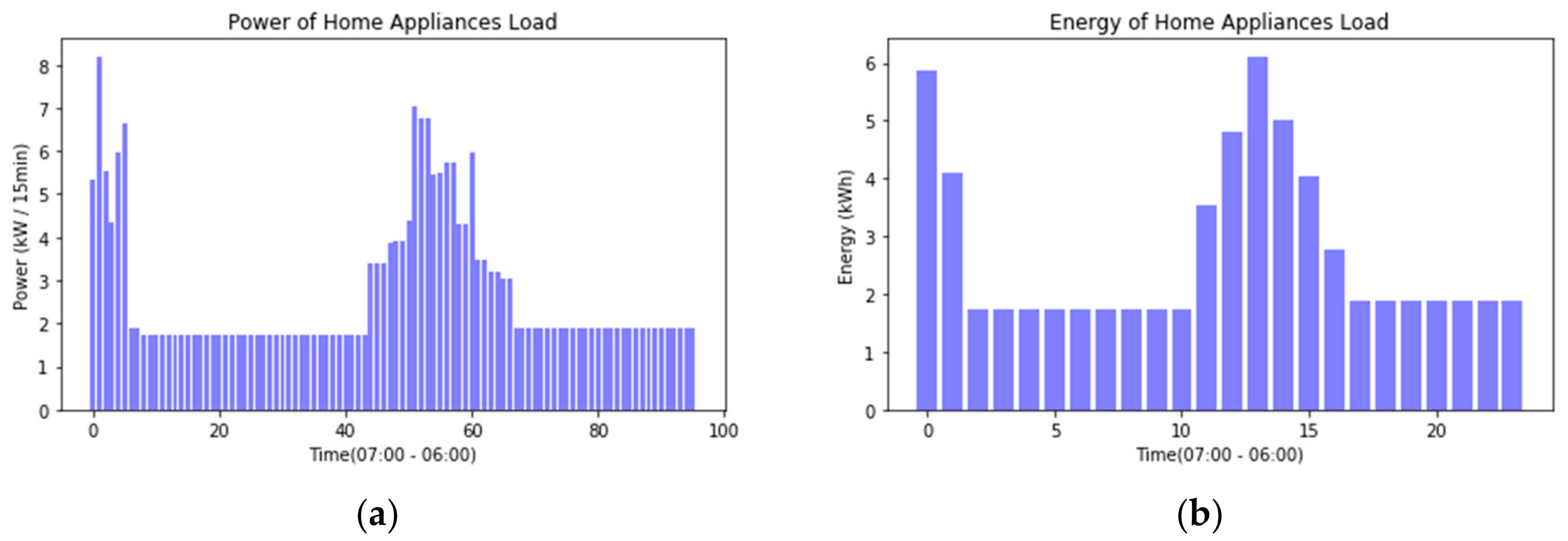
The home appliance usage pattern was modeled based on the smart home residents who woke up at 7 a.m. to prepare to go to work, and returned home to spend a their evenings with their family after 6 p.m. Figure 1 presents the graph of the usage pattern of home appliances during a day that models power consumption in 15-min increments.

Most power usage is concentrated before and after work, and it is known that only the standby power is consumed during the daytime when all family members are away from home. If the energy management system intervenes to control the load, a washing machine or dishwasher that can shift the time of day will run at dawn or daytime [20]. This method appears to use energy efficiently when analyzing only a change in energy consumption pattern, but there is the drawback that it may cause user inconvenience.

2.2. Modeling of Photovoltaic Generation System

The PV generation system of the smart home is limited in installation environment and size. In high-rise buildings, a building integrated photovoltaic generation system may be more advantageous than installing a PV generation system on the roof. In a single-story building, installing a PV generation system on the roof can be more cost and energy efficient. Partial degradation due to surrounding environment such as buildings and roadside trees should also be considered. In addition, PV generation is fundamentally proportional to the amount of solar radiation, so seasonal and climatic effects should be considered.

In this paper, the output power of PV generation system is modeled according to four weather conditions. The four weather conditions are sunny days, cloudy days, overcast days, and rainy days. The PV output model is based on data collected directly from an 100 W PV panel. Data was collected in May 2014 in Dong-Jak-Gu, Seoul, Korea. Figure 2 shows the output of PV generation system by weather. The day with the highest output of the PV generation system is on sunny days, and the output decreases slightly on cloudy days. On overcast days, the output of the PV generation system fluctuates strongly, and on rainy days it is assumed that there is no output power. In the simulation, the output of the PV generation system based on the 100 W panel is scaled up in accordance with the assumed smart home environment.

2.3. Modeling of Energy Storage System

Generally, a large capacity ESS connected to an energy network plays a role of storing surplus energy and providing that energy when the power supply is unstable. If the goal is economic benefit, the ESS is charges when the energy cost is cheap, and discharges when the energy cost rises and provides the profit to the operator. ESSs linked to renewable energy sources, such as PV generation systems or wind power generation systems, also function as energy buffers that keep outputs of environmentally-affected irregular renewable energy sources constant. That is, the ESS in the energy network serves as a load when charging and serves as an energy source when discharging.

The ESS model for the simulation of the proposed algorithm consists of the total energy capacity, the initial energy capacity, the efficiency of charge and discharge, and the maximum input and output power during the unit time. It is assumed that the lowest energy limit value to prevent the full discharge of the ESS is reflected. The percentage of dischargeable energy of the ESS is defined as the State of Charge (SoC), and the percentage of chargeable energy is defined as 1-SoC. Assume that the total energy capacity of the ESS is ESS_E, the initial energy amount is ESS_I, the charge and discharge power is ESS_P, the efficiency is 95%, and the unit time is 15 min. Here, the energy to be charged at the first time is as shown in Equation (1), and the energy to be discharged can be expressed as Equation (2). Equation (3) represents the current energy of the ESS_n which increases or decreases each time it is charged or discharged. The P means the charge and discharge parameter, and has a value of 1 when the ESS is charged, and a value of −1 when the ESS is discharged.

ESS_C = ESS_Init + (ESS_P × 0.95) × 15 min/60 min

(1)

ESS_D = ESS_I − (ESS_P/0.95) × 15 min/60 min

(2)

ESS_n = ESS_n−1 + ((1 + P)/2) × ESS_C + ((1 − P)/2) × ESS_D

(3)

2.4. T-A-P Algorithm

As mentioned above, the ESS in the smart home environment also serves as an energy buffer to reduce energy costs or to make unstable output consistent with the PV generation system. When it is aimed at cost reduction, it will discharge when the energy cost is expensive, and charge when it is cheap. However, in general, the daytime demand power rate is higher than that of the nighttime, and it is difficult to obtain a great effect in the foregoing case of the usage pattern of the home appliance load of the smart home. In addition, when simply used in conjunction with an energy storage for renewable energy, there is a disadvantage in that it can’t effectively utilize the ESS due to uneven power generation depending on the region and climate. Frequent charging and discharging to stabilize the energy network not only reduces the lifetime of the battery but also causes a considerable energy leak due to energy conversion, and thus is not a best operating method. That is, the operation method of charging and discharging for a certain period during a day according to the time schedule may be efficient when considering the battery cycle, but it is not an ideal method of operating the ESS as a load and an energy source. The method of simple utilization in connection with the renewable energy source is also insufficient to be the best method, considering the convenience in the smart home and the efficiency of the energy network.

Predictable energy consumption and supply information of a smart home enables sustainable energy network operation, so that smart home also improves energy sustainability. The most ideal sustainable energy network is a power network where demand and supply ratios remain constant. This means that the energy network operates at optimal cost and efficiency. This provides economic benefits to both users and utilities. Therefore, in this paper, we propose a T-A-P algorithm for optimal operation of smart home ESS. The primary goal of the proposed algorithm is to provide stable power to the appliances load. In other words, rather than recommending users to use home appliances at according to energy or cost savings, priority is placed on preventing users from recognizing the inconvenience of energy use. The ultimate goal of the proposed algorithm is to optimally control the ESS in a smart home space with a small ESS, a consumer electronics load, and a PV generation system. One assumption is needed to determine the charging and discharging of the ESS by the proposed algorithm. Assuming that the energy cost produced by the PV generation system and the energy cost stored in the ESS are lower than the energy network, this energy is preferentially supplied to the appliances load. In other words, this is a hypothesis to reduce the burden on the energy network by first consuming the self-supplied energy source.

As shown in Figure 3, there is a total of four cases when there is “A” demanding energy, “P” supplying energy, and the operating target power “T” of the ESS. The first is when A − P is less than or equal to 0, and the second is when A − P is less than T. The third is when A − P is equal to T, and the last is when A − P is greater than T. The following figure depicts each situation. Determination of charging and discharging, or waiting command during the unit time in accordance with four conditions and calculation of the detailed charging and discharging energy are described from the next paragraph.

2.4.1. (A − P) ≤ 0

When A − P is less than or equal to 0, PV power is equal to or greater than the power required by appliances. In other words, it is possible to drive household appliances with only PV generation, and residual energy can be supplied to the ESS.

• When ESS_SoC = 1

If the SoC of the ESS is 1, or 100% fully charged, the ESS and the energy network are not required to perform any operation. If the energy generated by the smart home can be supplied to the energy network, the P − A power can be converted into energy for a unit of time and supplied to the energy network. In such a situation, the formula summarizing the algorithm is Equation (4). The sign “←” means that energy comes in.

ESS = 0, EN = 0 or EN ← (P − A) × U_T

(4)

If the ESS is not 100% charged, it is divided into two situations where it is fully charged within a unit time and a situation where it is not fully charged even when the maximum charge is performed per unit time. That is, 1 − SoC × ESS_E can be divided into the case where 1 − SoC × ESS_E is larger than or equal to the energy amount multiplied by ESS_P and the unit time, and the case is small.

• When (1 − ESS_SoC) × ESS_E ≥ ESS_P × U_T

First, there is a time when P − A is greater than or equal to ESS_P and when P − A is less than ESS_P. If P − A is smaller than ESS_P, the power available to the user can be defined as T + P − A considering the operating target power T. This power is divided into the case where it is greater than or equal to ESS_P and the case where it is small. In summary, if P − A ≥ ESS_P, then the ESS is charged by ESS_P times the unit time, and the energy network does not supply any energy to the load. However, if the surplus energy can be supplied to the energy network, the energy network is supplied with the energy multiplied by the unit time of P − A − ESS_P (Equation (5)). If P − A is less than ESS_P and T + P − A is greater than or equal to ESS_P, then the ESS_P times the unit time is charged to the ESS. Here, the energy network supplies ESS_P − (P − A) times the unit time to the smart home (Equation (6)). If P − A is smaller than ESS_P and T + P − A is smaller than ESS_P, then the ESS is charged with T + P − A times the unit time. In this situation, the energy network supplies energy to the smart home by multiplying the operating target power by the unit time (Equation (7)). The following formula summarizes the above. The sign “→” means that energy goes out.

If (P − A) ≥ ESS_P

ESS ← ESS_P × U_T, EN = 0 or EN ← (P − A − ESS_P) × U_T

(5)

If ((P − A) < ESS_P) & (T + P − A ≥ ESS_P)

ESS ← ESS_P × U_T, EN → (ESS_P − (P − A)) × U_T

(6)

If ((P − A) < ESS_P) & (T + P − A < ESS_P)

ESS ← (T + P − A) × U_T, EN → T × U_T

(7)

• When (1 − ESS_SoC) × ESS_E < ESS_P × U_T

If it is possible to fully charge the ESS within the unit time, it may be effective to not operate the ESS in consideration of a decrease in battery lifetime due to frequent charging and discharging. However, since the purpose of this paper is to maximize the ESS, the operation required for the ESS is also defined. In this situation, the chargeable energy in the ESS may be equal to or greater than the energy multiplied by the unit time of P − A, and may also be less than this. In the first case, the ESS is charged by multiplying P − A by the unit time, and the energy network does not supply any energy (Equation (8)). In the second case, the ESS is charged until it is fully charged, and the energy network also does nothing. If the energy network can be supplied with residual energy, it can supply the difference between the energy multiplied by the unit time of P − A and the energy stored in the ESS (Equation (9)).

If (1 − ESS_SoC) × ESS_E ≥ (P − A) × U_T

ESS ← (P − A) × U_T, EN = 0

(8)

If (1 − ESS_SoC) × ESS_E < (P − A) × U_T

ESS ← (1 − ESS_SoC) × ESS_E, EN = 0 or EN ← (P − A) × U_T − (1 − ESS_SoC) × ESS_E

(9)

2.4.2. (A − P) < T

When A − P is smaller than T, the energy required by the load is smaller than the available limited energy, so it is possible to supply the load and charge the remaining energy to the ESS. In this case, three situations need to be considered.

• When ESS_SoC = 1

The first situation is when the ESS is 100% fully charged so there is no energy to charge to the ESS, and only the PV energy and energy networks supply the energy required by the load (Equation (10)).

ESS = 0, EN → (A − P) × U_T

(10)

• When (1 − ESS_SoC) × ESS_E ≥ ESS_P × U_T

The second situation is when the energy of the ESS that needs to be charged is greater than or equal to the ESS_P times the unit time. In this case, T + P − A is divided into the case where it is greater than or equal to ESS_P and the case where it is smaller. First, when T + P − A ≥ ESS_P, ESS is supplied with ESS_P times the unit time, and the energy network supplies ESS_P + (A − P) times the unit time to the smart home (Equation (11)). If T + P − A is less than ESS_P, the ESS is charged to T + P − A times the unit time, and the energy network supplies the energy multiplied by T times the unit time (Equation (12)).

If (T + P) − A ≥ ESS_P

ESS ← ESS_P × U_T, EN → (ESS_P + (A − P)) × U_T

(11)

If (T + P) − A < ESS_P

ESS ← ((T + P) − A) × U_T, EN → T × U_T

(12)

• When (1 − ESS_SoC) × ESS_E < ESS_P × U_T

Finally, the third situation is when the amount of energy in the ESS that needs to be charged is less than ESS_P times the unit time. This case is also divided into two conditions. First, when the amount of energy obtained by multiplying T + P − A by the unit time is smaller than the amount of energy required for charging, the energy obtained by multiplying T + P − A by the unit time is charged to the ESS. In this case, the energy network supplies energy to the smart home by multiplying the operating target power T by the unit time (Equation (13)). In the opposite case, the ESS is charged by the amount of energy required for charging, and the energy network supplies the amount of energy multiplied by A − P times the unit time minus the amount of energy charged to the ESS (Equation (14)). The situation when (1 − ESS_SoC) × ESS_E < ESS_P × U_T is summarized as follows.

If (1 − ESS_SoC) × ESS_E ≥ ((T + P) − A) × U_T

ESS ← ((T + P) − A) × U_T, EN → T × U_T

(13)

If (1 − ESS_SoC) × ESS_E < ((T + P) − A) × U_T

ESS ← (1 − ESS_SoC) × ESS_P, EN → (A − P) × U_T + (1 − ESS_SoC) × ESS_E

(14)

2.4.3. (A − P) = T

When A − P is equal to T, it is when the electric power required by home appliances load is supplied by PV generation system. In other words, the size of the insufficient power is equal to the operating target power. That is, when the usable power is P + T, the load of the home appliance is equal to P + T. Here, the ESS does not charge and discharge, and the energy network supplies energy that is the unit time multiplied by the operating target power T (Equation (15)). The situation when A − P is equal to T is presented as follows.

ESS = 0, EN → T × U_T

(15)

2.4.4. (A − P) > T

When A − P is larger than T, it is time to supply more energy to home appliances. It is necessary to use the ESS energy because the required power of the appliances load is larger than the operating target power which is the limit value. There are two cases in this situation. The current energy held by the ESS may be greater than or equal to the energy multiplied A − (T + P) by the unit time, or the value is smaller.

• When ESS_SoC × ESS_E ≥ (A − (T + P)) × U_T

In the first case, A − (T + P) can be divided into two cases: greater than or equal to ESS_P, and smaller. If A − (T + P) is greater than or equal to ESS_P, the energy is multiplied by ESS_P times the unit time, and the energy network supplies the energy to the smart home by multiplying A − P − ESS_P by the unit time (Equation (16)). When A − (T + P) is less than ESS_P, the ESS discharges energy by multiplying A − (T + P) by the unit time, and the energy network supplies energy to the smart home multiplied the operation target power by the unit time (Equation (17)).

If A − (T + P) ≥ ESS_P

ESS → ESS_P × U_T, EN → (A − P − ESS_P) × U_T

(16)

If A − (T + P) < ESS_P

ESS → (A − (T + P)) × U_T, EN → T × U_T

(17)

• When ESS_SoC × ESS_E < (A − (T + P)) × U_T

In the second case, there are two cases when the energy obtained by multiplying A − (T + P) by the unit time is larger than the energy of the ESS. When the energy of the ESS is greater than the energy multiplied by the unit time to the ESS_P, the ESS supplies energy to the smart home multiplied by the unit time to the ESS_P. Here, the energy network supplies energy to the smart home by multiplying A − P − ESS_P by the unit time (Equation (18)). When the energy of the ESS is less than the energy multiplied by the unit time of the ESS_P, the ESS discharges all of the energy it holds, and the energy network supplies the remaining energy excluding the energy discharged by the ESS from the energy multiplied A − P by the unit time (Equation (19)). If the ESS discharges all energy, it is assumed that the deep discharge limit for battery protection is already taken into account.

If ESS_SoC × ESS_E ≥ ESS_P × U_T

ESS → ESS_P × U_T, EN → (A − P − ESS_P) × U_T

(18)

If ESS_SoC × ESS_E < ESS_P × U_T

ESS → ESS_SoC × ESS_E, EN → (A − P) × U_T − (ESS_SoC × ESS_E)

(19)

3. Simulation and Results

To simulate the proposed T-A-P algorithm, we assumed a smart home environment with 28 appliances, a PV generation system, and an ESS. As mentioned earlier, smart home appliances were modeled with usage patterns starting at 7 a.m. It is also assumed that a smart home has a 5 kW PV generation system and an ESS of 13.2 kWh. The power conversion efficiency of the ESS is assumed to be 95%, the initial energy storage capacity is 50% of the total capacity, and the maximum input/output power is 2.5 kW. The unit time of the simulation is 15 min, and a total of 96 cases are judged for 24 h. The operating target power was varied from 0.5 kW to 8.0 kW and the operating results of the algorithm were observed. In order to observe the change of the optimal T value according to the influence of the output of the PV generation system, the results were derived by changing the PV output power based on the four weather conditions. The simulation was implemented in the Jupyter Notebook environment and used Python programming language.

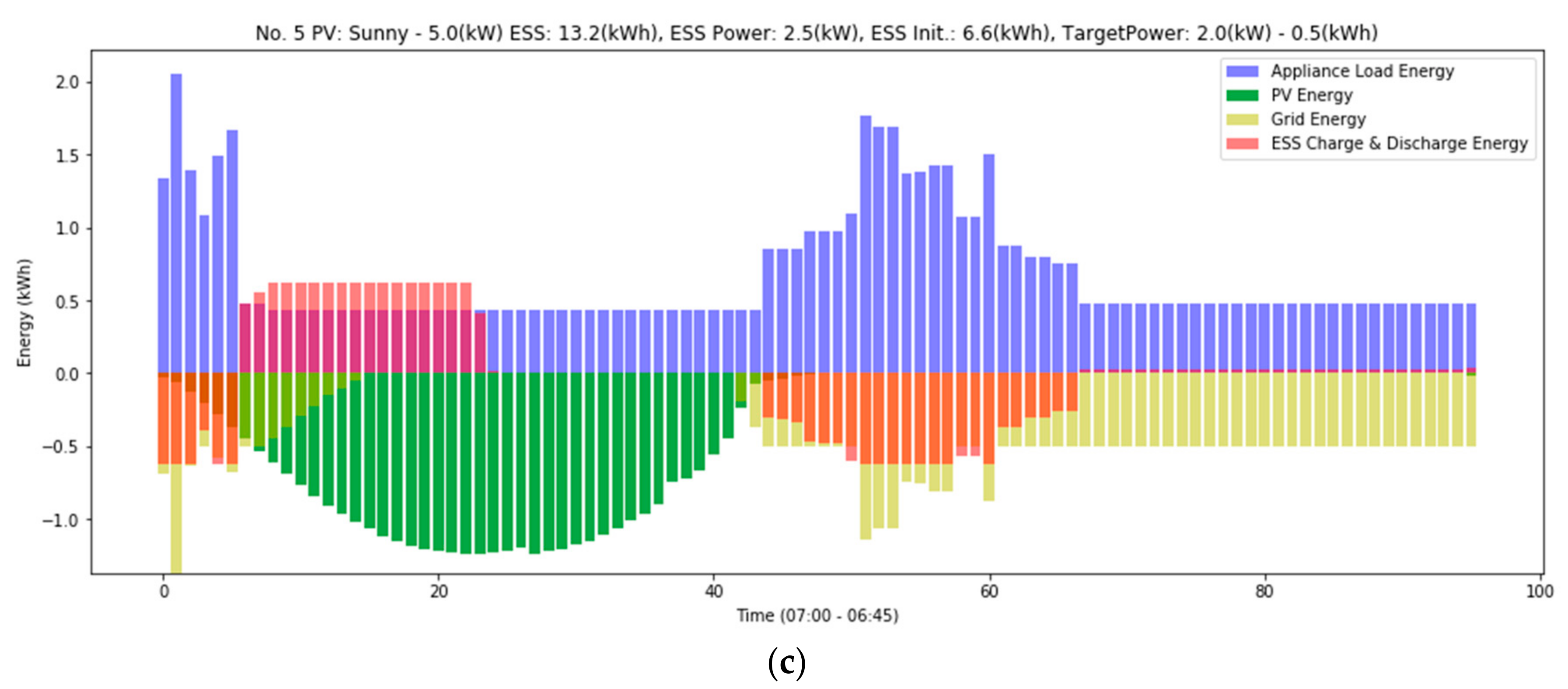
The ideal result of the proposed algorithm is that the ESS properly performs charging and discharging regardless of energy generation by PV, which then reduces the energy burden on the energy network or makes the energy consumption pattern constant. Figure 4 presents a typical graph of results according to simulation conditions. In the graph, a positive value indicates energy consumption and a negative value indicates energy production. That is, if ESS has a positive value, it is a charged load, and if it has a negative value, it is a discharging energy source.

The first result graph shows that the ESS alternates between charging and discharging but is not steady. In other words, ESS only worked in less than half of the 96 simulation runs per day. It can also be seen that the energy supplied by the energy network does not have a constant size in the latter part of the simulation. This means that in terms of the energy supplier, the load varies over time and is more volatile than a load of constant magnitude.

In the second result graph, the number of charge and discharge cycles of ESS is the same as the first graph. However, since ESS is used throughout most of the time domain, it can be seen that ESS is used more actively than the first result graph. This means that the utilization of the ESS is higher than the first simulation condition without changing the battery cycle by the number of charge and discharge times. Also, it can be seen that the energy supply pattern of the energy network in the latter half is kept constant. In other words, the ESS plays a role of a constant load by storing the remaining energy in a stable time of energy supply. From an energy provider’s viewpoint, this means that a demand-supply curve with a bend can change to a flat curve. In addition, it is expected that energy network operators will benefit not only from the sustainability of the energy network but also from the operating cost because it enables more efficient operation in determining the power generation amount in order to secure the power reserve ratio.

The third graph shows the results when the operating target power is smaller. Compared to the first graph, it can be seen that the ESS is driven more, and has more charged and discharged energy, and the energy network also supplies a constant energy to the smart home. However, compared to the second graph, a smaller amount of energy is being supplied. In addition, it is difficult to judge that better results are obtained because the difference between the constant supply of the energy network and the largest is greater than the second result graph.

As can be seen from the three representative results derived from changing the simulation conditions, there is an optimal T value according to the energy generation and consumption conditions of the smart home. Based on this analysis, we defined a cost function to find the optimal T value of the proposed algorithm. The cost function is expressed as the average of the energy charged and discharged to the ESS minus the number of times the absolute value of the difference between the power supplied by the energy network and the operating target power. The use of ESS is a positive indicator, so it is added in the cost function. On the other hand, the fact that T − EN is far from 0 indicates that it is a negative index, so it was subtracted from the cost function. The following Equation (20) shows the cost function for finding the appropriate target power in this paper. The ESS_CE and ESS_CC are charging energy and count of ESS. The ESS_DE and ESS_DC are discharging energy and count of ESS. The |T−EN|_E means absolute difference energy between target power and power of energy network, and the |T−EN|_C means absolute number of count when target power is not equal to power of energy network.

Cost Function = Avg(ESS_CE × ESS_CC + ESS_DE × ESS_DC) − (|T−EN|_E × |T−EN|_C)

(20)

Table 2. Results of the cost function while changing the T from 5 to 1.

Target Power	5	4.5	4	3.5	3	2.5	2	1.5	1
|T−EN|E	2.62	4.75	8.63	8.13	13.86	18.09	17.67	43.91	42.66
|T−EN|c	1	2	4	4	8	12	13	46	52
ESSCE	10.23	11.84	13.49	15.50	18.06	15.07	11.63	10.98	11.10
ESSDE	2.97	4.42	5.91	7.72	10.04	12.43	14.47	16.18	16.29
ESSCC	23	27	30	37	47	47	48	20	21
ESSDC	12	13	16	20	29	29	29	29	28
Cost Function	132.9	179.1	215.2	331.4	459.2	317.3	259.2	−1675.5	−1873.9
Best Cost = 459.2, Weather = Sunny, when PV: 5.0 kW ESSE: 13.2 kWh, ESSP: 2.5 kW, ESSInit: 6.6 kWh.
|T−EN|E	2.63	4.77	8.64	8.14	15.47	19.64	18.02	44.36	43.92
|T−EN|c	1	2	4	4	9	13	13	46	53
ESSCE	10.56	12.21	13.87	15.92	18.43	15.17	11.68	11.04	11.10
ESSDE	3.26	4.75	6.25	8.11	10.37	12.58	14.58	16.23	16.29
ESSCC	23	28	31	38	47	48	49	22	23
ESSDC	13	13	16	20	29	29	29	32	29
Cost Function	140.0	192.2	230.3	351.0	444.4	291.1	263.3	−1659.5	−1963.7
Best Cost = 444.4, Weather = Cloudy, when PV: 5.0 kW ESSE: 13.2 kWh, ESSP: 2.5 kW, ESSInit: 6.6 kWh.
|T−EN|E	2.64	4.78	8.65	8.15	15.49	19.72	18.09	52.96	53.86
|T−EN|c	1	2	4	4	9	13	13	51	55
ESSCE	10.64	12.29	13.94	16.05	18.53	15.21	11.12	5.89	3.25
ESSDE	3.33	4.82	6.32	8.21	10.46	12.61	14.61	11.59	9.20
ESSCC	24	28	33	40	48	54	67	30	17
ESSDC	13	13	16	20	29	29	29	28	33
Cost Function	146.7	193.8	245.9	370.5	457.1	337.1	349.2	−2450.5	−2782.6
Best Cost =457.1, Weather = Overcast, when PV: 5.0 kW ESSE: 13.2 kWh, ESSP: 2.5 kW, ESSInit: 6.6 kWh.
|T−EN|E	2.67	4.81	10.72	10.09	18.82	20.15	32.80	66.30	76.30
|T−EN|c	1	2	5	5	11	13	21	58	83
ESSCE	11.08	12.73	14.44	16.43	18.77	11.61	3.24	0.00	0.00
ESSDE	3.73	5.22	6.76	8.56	10.74	12.78	8.49	6.27	6.27
ESSCC	24	29	32	46	64	67	67	0	0
ESSDC	13	13	17	20	29	29	16	45	20
Cost Function	154.5	208.8	235.0	412.9	549.3	312.2	−512.5	−3704.2	−6270.2
Best Cost = 549.3, Weather = Rainy, when PV: 5.0 kW ESSE: 13.2 kWh, ESSP: 2.5 kW, ESSInit: 6.6 kWh.

shows the result of calculating the cost function while changing the T from 5 to 1 to obtain the optimal T value when the consumption pattern of the home appliances and the PV output according to the weather are the same.

The results show that the interval between the T values is set at 0.5 and the optimal T is 3 although the PV output varies depending on the weather. When the home appliance load, 5 kW PV generation system, and ESS of 13.2 kWh are in the smart home, operating the ESS’s target power of 3 kW will not only make maximum use of the ESS, but also cause the smart home to consume a certain amount of energy in the energy network. It means that it can serve as a load. In addition, it is advantageous to use the energy cost effectively by operating the ESS of the smart home based on the optimal operating target power even in the variable rate by the energy use restriction like the demand charge instead of the time varying charge system.

Assuming that the interval of T is set to 0.25, the capacity of ESS is 3.3 kWh and 6.6 kWh, and 1 kW, 3 kW, 5 kW PV generation system is installed, and the same appliances load exist in the smart home,

Table 3. Simulation results when the interval of T (Target Power) is 0.25.

ESSE	PV		T	ESSE	PV		T	ESSE	PV		T
3.3 kWh	1 Kw	Sunny	4.5	3.3 kWh	5 kW	Sunny	4.5	6.6 kWh	3 kW	Sunny	3.25
3.3 kWh	1 kW	Cloudy	4.75	3.3 kWh	5 kW	Cloudy	4.5	6.6 kWh	3 kW	Cloudy	3.5
3.3 kWh	1 kW	Overcast	4.75	3.3 kWh	5 kW	Overcast	4.5	6.6 kWh	3 kW	Overcast	3.25
3.3 kWh	1 kW	Rainy	4.5	3.3 kWh	5 kW	Rainy	4.5	6.6 kWh	3 kW	Rainy	3.5
3.3 kWh	3 kW	Sunny	4.5	6.6 kWh	1 kW	Sunny	3.25	6.6 kWh	5 kW	Sunny	3.25
3.3 kWh	3 kW	Cloudy	4.5	6.6 kWh	1 kW	Cloudy	3.5	6.6 kWh	5 kW	Cloudy	3.25
3.3 kWh	3 kW	Overcast	4.5	6.6 kWh	1 kW	Overcast	3.5	6.6 kWh	5 kW	Overcast	3.25
3.3 kWh	3 kW	Rainy	4.5	6.6 kWh	1 kW	Rainy	3.5	6.6 kWh	5 kW	Rainy	3.5

Optimal operating target power “T” when PV: 1 kW and 5 kW, ESS_E: 3.3 kWh and 6.6 kWh.

shows the optimal T value according to each condition. Unlike previous simulations, we found that optimal T was present by varying the capacity of PV generation system and ESS.

As the variation interval of T decreased, the optimal T value with slight difference was derived for each weather condition. However, when T was 4.5 and 4.75, the difference in the cost function was not significant. Also, as the capacity of the ESS doubles, the optimal T is reduced by about one. In the previous simulation, we can conclude that the optimal T is 3 when the capacity of the ESS is 13.2 kWh, so that the relationship between the T, A, P variables and the energy storage system does not have a constant ratio. Also, using the algorithm proposed in this paper reversely, it is possible to calculate the optimal capacity of PV generation system and ESS inversely when we can know the load usage pattern of appliances in smart home. However, the user should make economical choices considering installation and maintenance costs that follow as the capacity of each system increases.

4. Discussion

Most EMSs have required changes in user energy usage patterns to remove unnecessary loads from the energy network or limit its use. This can cause user inconvenience as it requires behavioral adjustments in order to save energy. In this paper, we proposed and simulated the ESS control algorithm without user’s discomfort in a smart home equipped with a PV generation system and an ESS. In addition, when the proposed algorithm is applied to a smart home, from the viewpoint of the energy network, it plays the role of making the smart home a constant energy consuming load. The goal is to simplify energy network with uncertainty and complexity that are mixed with diverse energy providers and users. This helps energy providers to provide a stable supply of energy and is directly related to the maintenance costs of the energy network.

From the simulation results of the proposed algorithm, we confirm that the optimal operating target value exists. In the future, it is expected that there will be many smart homes with different energy conditions depending on the user’s living environment, house size, and living pattern. There are problems that need to be solved in order for the proposed algorithm to be practically implemented in these diverse environments. In the simulation, the algorithm is applied based on the data for the unit time, and the result is derived. However, in reality, it is necessary to predict the power consumption of the next unit time and to determine the charging and discharging of the ESS by reflecting the error to the algorithm.

In addition, in this paper, we do not make assumptions about the tariff system to interpret and prove the pure role and function of the proposed algorithm. In order to maximize the benefit to the users in conjunction with the tariff system or to operate the ESS for the future energy prosumer, the proposed algorithm should apply the electricity tariff system. In the current research stage, the optimal tariff system will be a demand charge method in which the charge is lowered to a limited amount of electric power consumption and the charge rises when the limited use amount is exceeded. In order to derive more advanced research results, it is necessary to apply various tariff system such as real time price, time of use and day ahead pricing to smart home composed of ESS, EV and PV generation systems. Future research will therefore proceed to algorithms that select the best available energy sources in a more complex smart home environment.

5. Conclusions

A future sustainable smart space should be able to provide valuable services to people. As energy and environmental concerns are increasing worldwide, a variety of technologies and services are emerging. In addition, as the de-nuclear era is being discussed in the international society, research and development on sustainable energy and environment are accelerating. Traditionally, smart home was a space where human beings lived, and simultaneously acted as a new technology test bed. There have been various efforts to solve social problems centered on smart home, and the latest technologies, which are now attracting attention, are developing around smart homes.

Recently, the smart home is shifting to smart space that solves potential societal problems related with energy and environment. In terms of energy and environment, the smart space can be defined as a service domain that can supply sustainable energy in an environmentally friendly way, and many smart homes can be viewed as a logical aggregate of mesh structures. At the heart of this paradigm shift are information and communication technologies (ICT) and energy storage technologies. Internet of Things, one of the ICT, is helping to reduce the cost and time by visualizing invisible information and linking objects or things. Typical energy technologies are ESSs, and the future smart space will be equipped with various forms of energy storage to efficiently manage energy.

ESSs are generally used to offer direct benefit to users. In other words, the ESS provides users with a choice of energy and cost savings by adjusting the peak load, or by comparing the energy cost of the energy network with the stored energy cost. In this paper, we have proposed and simulated the algorithm for maximizing the use of ESS installed in a smart home equipped with a PV generation system that produces eco-friendly energy. Due to the basic characteristics of ESS such as modularity, scalability, and fast response, this study could propose a new way to utilize ESS. With the advent of diverse energy consumption entities and distributed energy resources, the energy network is becoming more and more complex. From the past, smart home has always been a test bed that is the center of our lives, so we have proposed an algorithm that can be a load of energy network with new features such as low uncertainty and complexity. We also have defined the role and function of the smart space to evolve into a key component of the future sustainable energy network, rather than function as a mere living space and smart space for receiving automation services.