Calculation of Characterization Factors of Mineral Resources Considering Future Primary Resource Use Changes: A Comparison between Iron and Copper


Abstract
:1. Introduction
- The building up of infrastructure in rapidly developing economies will cause continuously-rising demand for steel and other base metals.
- The electronics revolution, expressed in products like smartphones, flat screen televisions, or USB sticks, is leading to growing demand for many minor and precious metals.
- The shift towards renewable energy technologies, like wind and photovoltaic energy, will contribute to increased global metal demand.
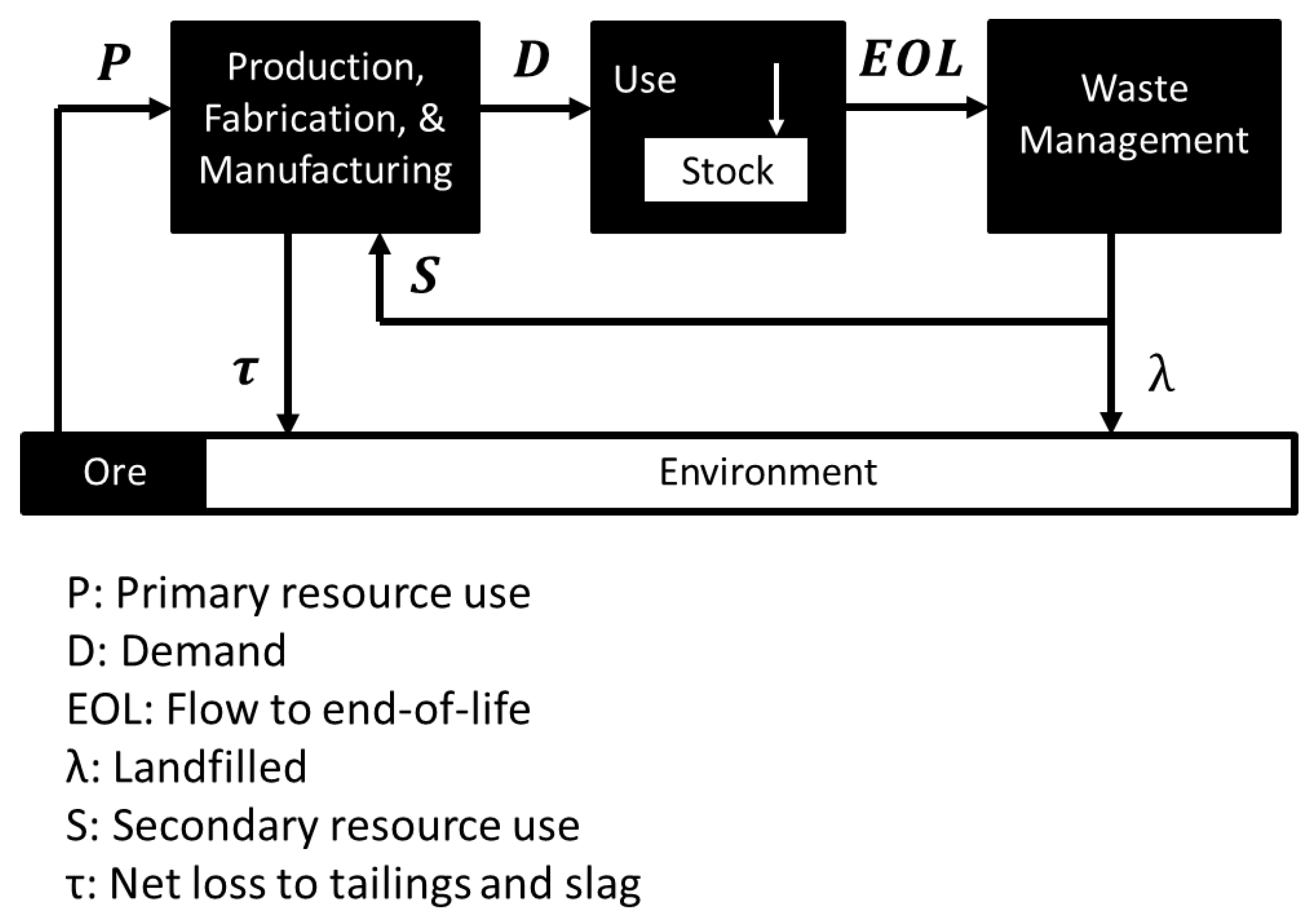
2. Model
2.1. Demand Change-Based Surplus Cost
2.2. Time-Series Primary Resource Use
2.3. Future Total Demand
3. Parameter Estimation
3.1. Yield Rate
3.2. Historical Total Demand
3.3. Recycling Rate
3.4. Lifetime Distribution
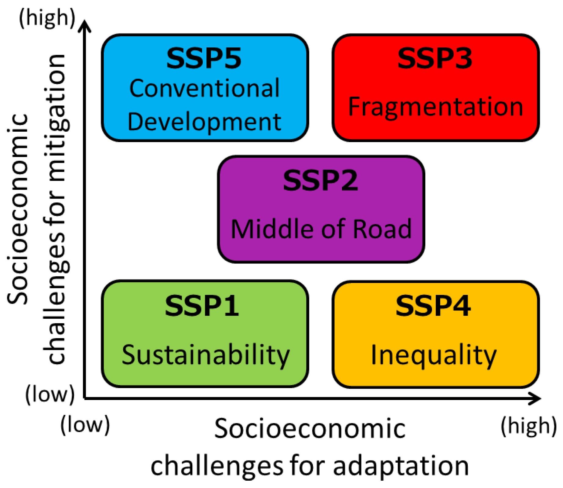
3.5. Future Scenarios
4. Results
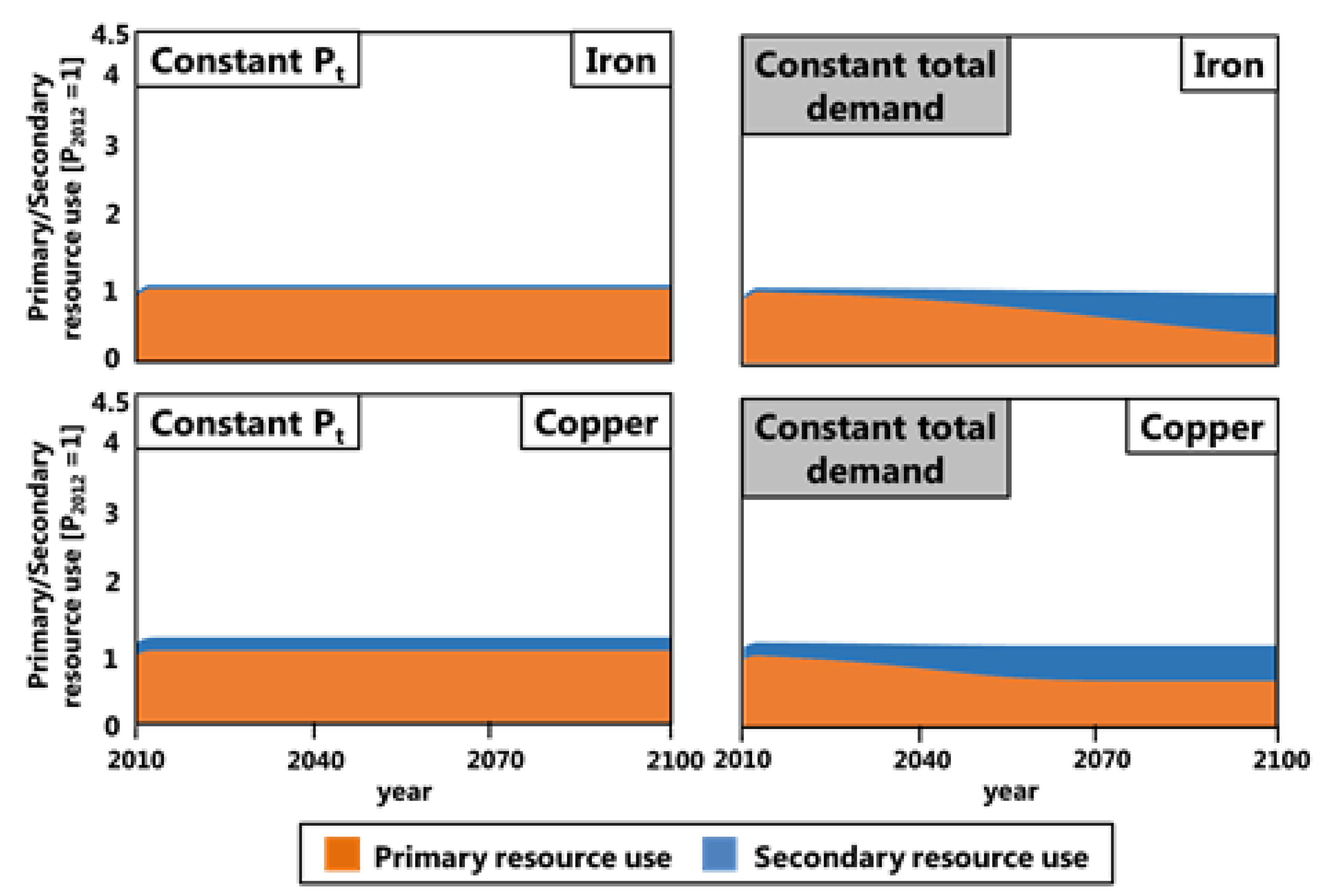
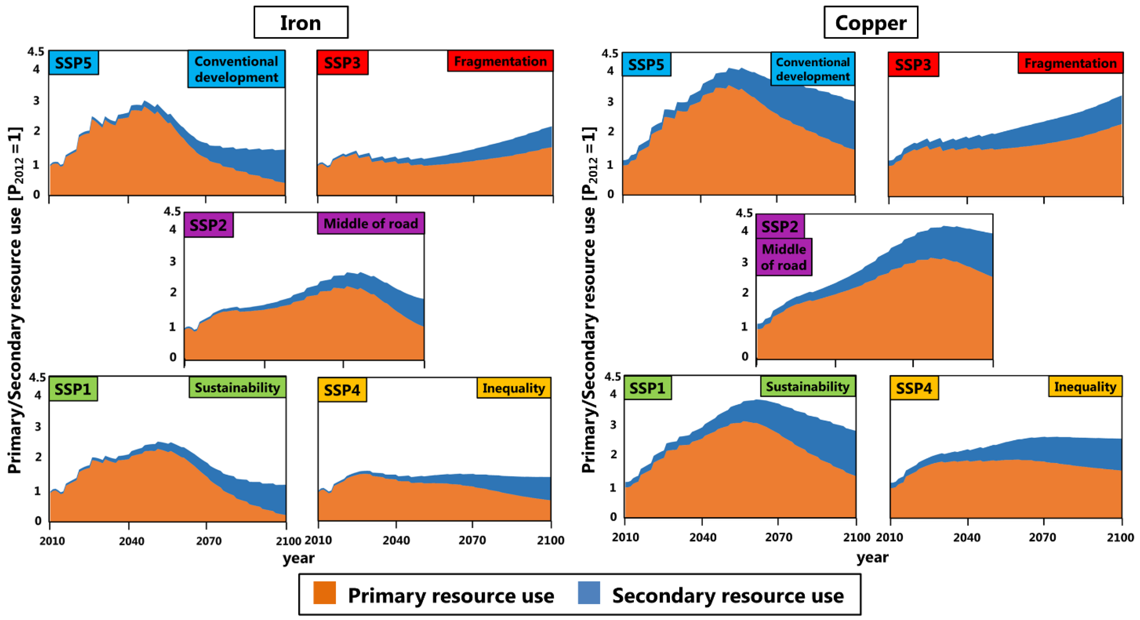
4.1. Time-Series Primary Resource Use
4.2. Demand Change-Based Surplus Cost
4.3. Sensitivity Analysis
5. Discussion
6. Conclusions
Acknowledgments
Author Contributions
Conflicts of Interest
References
- Allwood, J.M.; Cullen, J.M.; Milford, R.L. Options for achieving a 50% cut in industrial carbon emissions by 2050. Environ. Sci. Technol. 2010, 44, 1888–1894. [Google Scholar] [CrossRef] [PubMed]
- Gordon, R.B.; Bertram, M.; Graedel, T.E. Metal stocks and sustainability. Proc. Natl. Acad. Sci. USA 2006, 103, 1209–1214. [Google Scholar] [CrossRef] [PubMed]
- Prior, T.; Daly, J.; Mason, L.; Giurco, D. Resourcing the future: Using foresight in resource governance. Geoforum 2013, 44, 316–328. [Google Scholar] [CrossRef]
- Tilton, J.E.; Lagos, G. Assessing the long-run availability of copper. Resour. Policy 2007, 32, 19–23. [Google Scholar] [CrossRef]
- Gerst, M.D.; Graedel, T.E. In-use stocks of metals: Status and implications. Environ. Sci. Technol. 2008, 42, 7038–7045. [Google Scholar] [CrossRef] [PubMed]
- United Nations Environment Programme (UNEP). Environmental Risks and Challenges of Anthropogenic Metals Flows and Cycles (Summary); UNEP: Paris, France, 2013. [Google Scholar]
- Finnveden, G.; Hauschild, M.; Ekvall, T.; Guinée, J.; Heijungs, R.; Hellweg, S.; Koehler, A.; Pennington, D.; Suh, S. Recent developments in Life Cycle Assessment. J. Environ. Manag. 2009, 91, 1–21. [Google Scholar] [CrossRef] [PubMed]
- Yellishetty, M.; Ranjith, P.G.; Tharumarajah, A.; Bhosale, S. Life cycle assessment in the minerals and metals sector: A critical review of selected issues and challenges. Int. J. Life Cycle Assess. 2009, 14, 257–267. [Google Scholar] [CrossRef]
- Drielsma, J.A.; Allington, R.; Brady, T.; Guinée, J.; Hammarstrom, J.; Hummen, T.; Russell-Vaccari, A.; Schneider, L.; Sonnemann, G.; Weihed, P. Abiotic Raw-Materials in Life Cycle Impact Assessments: An Emerging Consensus across Disciplines. Resources 2016, 5, 12. [Google Scholar] [CrossRef]
- Berger, M.; Sonderegger, T. Harmonizing the assessment of resource use in LCA—First results of the task force on natural resources of the UNEP-SETAC global guidance on environmental life cycle impact assessment project. In Proceedings of the SETAC Europe 27th Annual Meeting, Brussels, Belgium, 7–11 May 2017. [Google Scholar]
- Steen, B.A. Abiotic resource depletion: Different perceptions of the problem with mineral deposits. Int. J. Life Cycle Assess. 2006, 11, 49–54. [Google Scholar] [CrossRef]
- Guinée, J.B.; Heijungs, R. A proposal for the definition of resource equivalency factors for use in product life-cycle assessment. Environ. Toxicol. Chem. 1995, 14, 917–925. [Google Scholar] [CrossRef]
- Dewulf, J.; Bösch, M.E.; de Meester, B.; van der Vorst, G.; van Langenhove, H.; Hellweg, S.; Huijbregts, A.J. Cumulative Exergy Extraction from the Natural Envionment (CEENE): A comprehensive Life Cycle Impact Assessment method for resource accounting. Environ. Sci. Technol. 2007, 41, 8477–8483. [Google Scholar] [CrossRef] [PubMed]
- Itsubo, N.; Inaba, A. LIME2: Life-Cycle Impact Assessment Method Based on Endpoint Modeling Chapter 2: Characterization and Damage Evaluation Methods. JLCA Newsletter No.18. 2014. Available online: http://lca-forum.org/english/pdf/No18_Chapter2.10-2.13.pdf (accessed on 23 December 2016).
- Goedkoop, M.; Heijungs, R.; Huijbregts, M.; de Schryver, A.; Struijs, J.; van Zelm, R. ReCiPe 2008: A Life Cycle Impact Assessment Method Which Comprises Harmonised Category Indicators at the Midpoint and the Endpoint Level, 1st ed.; Version 1.08, Report I: Characterisation; Ministry of Housing, Spatial Planning and the Environment (VROM): The Hague, The Netherlands, 2009.
- Steen, B.A. A Systematic Approach to Environmental Priority Strategies in Product Development (EPS). Version 2000—Models and Data of the Default Method; Chalmers University of Technology: Gothenburg, Sweden, 1999. [Google Scholar]
- Drielsma, J.A.; Russell-Vaccari, A.J.; Drnek, T.; Brady, T.; Weihed, P.; Mistry, M.; Simbor, L.P. Mineral resources in life cycle impact assessment—Defining the path forward. Int. J. Life Cycle Assess. 2016, 21, 85–105. [Google Scholar] [CrossRef]
- Klinglmair, M.; Sala, S.; Brandão, M. Assessing resource depletion in LCA: A review of methods and methodological issues. Int. J. Life Cycle Assess. 2014, 19, 580–592. [Google Scholar] [CrossRef]
- Sonderegger, T.; Dewulf, J.; Fantke, P.; de Souza, D.; Pfister, S.; Stoessel, F.; Verones, F.; Vieira, M.; Weidema, B.; Hellweg, S. Towards harmonizing natural resources as an area of protection in life cycle assessment. Int. J. Life Cycle Assess. 2017, 22, 1912–1927. [Google Scholar] [CrossRef]
- Alvarenga, R.A.F.; Lins, I.O.; de Almeida Neto, J.A. Evaluation of abiotic resource LCIA methods. Resources 2016, 5, 13. [Google Scholar] [CrossRef]
- Hauschild, M.; Goedkoop, M.; Guinée, J.B.; Heijungs, R.; Huijbregts, M.; Jolliet, O.; Margni, M.; Schryver, A.; Humbert, S.; Laurent, A.; et al. Identifying best existing practice for characterization modeling in life cycle impact assessment. Int. J. Life Cycle Assess. 2013, 18, 683–697. [Google Scholar] [CrossRef]
- Hauschild, M.; Goedkoop, M.; Guinee, J.; Heijungs, R.; Huijbregts, M.; Jolliet, O.; Margni, M.; De Schryver, A. Recommendations for Life Cycle Impact Assessment in the European context—based on existing environmental impact assessment models and factors (International Reference Life Cycle Data System—ILCD handbook); European Union: Brussels, Belgium, 2011. [Google Scholar]
- Ponsioen, T.C.; Viera, M.D.M.; Goedkoop, M.J. Surplus cost as a life cycle impact indicator for fossil resource scarcity. Int. J. Life Cycle Assess. 2014, 19, 872–881. [Google Scholar] [CrossRef]
- Vieira, M.D.M.; Ponsioen, T.C.; Goedkoop, M.J.; Huijbregts, M.A.J. Surplus cost potential as a life cycle impact indicator for metal extraction. Resources 2016, 5, 2. [Google Scholar] [CrossRef]
- Huijbregts, M.A.J.; Steinmann, Z.J.N.; Elshout, P.M.F.; Stam, G.; Verones, F.; Vieira, M.; Zijp, M.; Hollander, A.; van Zelm, R. ReCiPe2016 a harmonised life cycle impact assessment method at midpoint and endpoint level. Int. J. Life Cycle Assess. 2017, 22, 138–147. [Google Scholar] [CrossRef]
- Schneider, L.; Berger, M.; Finkbeiner, M. The anthropogenic stock extended abiotic depletion potential (AADP) as a new parameterisation to model the depletion of abiotic resources. Int. J. Life Cycle Assess. 2011, 16, 929–936. [Google Scholar] [CrossRef]
- Schneider, L.; Berger, M.; Finkbeiner, M. Abiotic resource depletion in LCA—Background and update of the anthropogenic stock extended abiotic depletion potential (AADP) model. Int. J. Life Cycle Assess. 2015, 20, 160–182. [Google Scholar] [CrossRef]
- USGS. Mineral Commodity Summaries. Available online: http://minerals.usgs.gov/minerals/pubs/mcs/ (accessed on 24 January 2016).
- Tilton, J.E. Exhaustible resources and sustainable development: Two different paradigms. Resour. Policy 1996, 22, 91–97. [Google Scholar] [CrossRef]
- Müller, E.; Hilty, L.M.; Widmer, R.; Schluep, M.; Faulstich, M. Modeling metal stocks and flows: A review of dynamic material flow analysis methods. Environ. Sci. Technol. 2014, 48, 2102–2113. [Google Scholar] [CrossRef] [PubMed]
- Graedel, T.E.; Barr, R.; Chandler, C.; Chase, T.; Choi, J.; Christoffersen, L.; Friedlander, E.; Henly, C.; Jun, C.; Nassar, N.T.; et al. Methodology of metal criticality determination. Environ. Sci. Technol. 2012, 46, 1063–1070. [Google Scholar] [CrossRef] [PubMed]
- Nuss, P.; Harper, E.M.; Nassar, N.T.; Reck, B.K.; Graedel, T.E. Criticality of Iron and Its Principal Alloying Elements. Environ. Sci. Technol. 2014, 45, 182–188. [Google Scholar] [CrossRef] [PubMed]
- Pauliuk, S.; Wang, T.; Müller, D.B. Steel all over the world: Estimating in-use stocks of iron for 200 countries. Resour. Conserv. Recycl. 2013, 71, 21–30. [Google Scholar] [CrossRef] [Green Version]
- Pauliuk, S.; Milford, R.L.; Müller, D.B.; Allwood, J.M. The Steel Scrap Age. Environ. Sci. Technol. 2013, 47, 3448–3454. [Google Scholar] [CrossRef] [PubMed] [Green Version]
- Gerst, M.D. Linking Material Flow Analysis and Resource Policy via Future Scenarios of In-Use Stock: An Example for Copper. Environ. Sci. Technol. 2009, 43, 6320–6325. [Google Scholar] [CrossRef] [PubMed]
- Nassar, N.T.; Barr, R.; Browning, M.; Diao, Z.; Friedlander, E.; Harper, E.M.; Henly, C.; Kavlak, G.; Kwatra, S.; Jun, C.; et al. Criticality of the Geological Copper Family. Environ. Sci. Technol. 2012, 46, 1071–1078. [Google Scholar] [CrossRef] [PubMed]
- Spatari, S.; Bertram, M.; Gordon, R.B.; Henderson, K.; Graedel, T.E. Twentieth century copper stocks and flows in North America: A dynamic analysis. Ecol. Econ. 2005, 54, 37–51. [Google Scholar] [CrossRef]
- Van Vuuren, D.P.; Strengers, B.J.; De Vries, H.J.M. Long-term perspectives on world metal use—A system-dynamics model. Resour. Policy 1999, 25, 239–255. [Google Scholar] [CrossRef]
- Müller, D.B.; Wang, T.; Duval, B. Patterns of iron use in societal evolution. Environ. Sci. Technol. 2011, 45, 182–188. [Google Scholar] [CrossRef] [PubMed]
- Müller, D.B.; Wang, T.; Duval, B.; Graedel, T.E. Exploring the engine of anthropogenic iron cycles. Proc. Natl. Acad. Sci. USA 2006, 103, 16111–16116. [Google Scholar] [CrossRef] [PubMed]
- Bader, H.-P.; Scheidegger, R.; Wittmer, D.; Lichtensteiger, T. Copper flows in buildings, infrastructure and mobiles: A dynamic model and its application to Switzerland. Clean Technol. Environ. Policy 2011, 13, 87–101. [Google Scholar] [CrossRef]
- Hatayama, H.; Daigo, I.; Matsuno, Y.; Adachi, Y. Outlook of the World Steel Cycle Based on the Stock and Flow Dynamics. Environ. Sci. Technol. 2010, 44, 6457–6463. [Google Scholar] [CrossRef] [PubMed]
- Wen, Z.; Zhang, C.; Ji, X.; Xue, Y. Urban Mining’s Potential to Relieve China’s Coming Resource Crisis. J. Ind. Ecol. 2015, 19, 1091–1102. [Google Scholar] [CrossRef]
- Wang, T.; Müller, D.B.; Graedel, T.E. Forging the Anthropogenic Iron Cycle. Environ. Sci. Technol. 2007, 41, 5120–5129. [Google Scholar] [CrossRef] [PubMed]
- Gordon, R.B. Production residues in copper technological cycles. Resour. Conserv. Recycl. 2002, 36, 87–106. [Google Scholar] [CrossRef]
- Kapur, A. The future of the red metal—A developing country perspective from India. Resour. Conserv. Recycl. 2006, 47, 160–182. [Google Scholar] [CrossRef]
- World Steel Association. Steel Statistical Yearbook. Available online: https://www.worldsteel.org/statistics/statistics-archive/yearbook-archive.html (accessed on 25 January 2016).
- USGS. Minerals Yearbook: Volume I. Metals and Minerals. Available online: http://minerals.usgs.gov/minerals/pubs/commodity/myb/ (accessed on 24 January 2016).
- UN Comtrade. Commodity Trade Statistics Database. Available online: http://comtrade.un.org/db/ (accessed on 24 January 2016).
- Nakamura, S.; Nakajima, K.; Kondo, Y.; Nagasaka, T. The Waste Input-Output Approach to Materials Flow Analysis. J. Ind. Ecol. 2007, 11, 50–63. [Google Scholar] [CrossRef]
- Ministry of Internal Affairs and Communications. 2011 Input-Output Tables for Japan. Available online: http://www.soumu.go.jp/english/dgpp_ss/data/io/io11.htm (accessed on 22 January 2016).
- USGS. Historical Statistics for Mineral and Material Commodities in the United States. Available online: http://minerals.usgs.gov/minerals/pubs/historical-statistics/ (accessed on 24 January 2016).
- Ayres, R.U.; Ayres, L.W.; Rade, I. The Life Cycle of Copper, Its Co-Products and By-Products, Mining, Minerals and Sustainable Development; International Institute for Environment and Development (IIED): London, UK, 2002. [Google Scholar]
- IIASA. SSP Database (Shared Socioeconomic Pathways) Version 1.0. Available online: https://tntcat.iiasa.ac.at/SspDb/dsd?Action=htmlpage&page=about (accessed on 25 January 2016).
- Maddison, A. The World Economy; OECD Development Centre Studies: Paris, France, 2006. [Google Scholar]
- United Nations. National Accounts Main Aggregates Database. Available online: http://unstats.un.org/unsd/snaama/Introduction.asp (accessed on 25 January 2016).
- Committee of Iron and Steel Statistics. Handbook for Iron and Steel Statistics; Japan Iron and Steel Federation: Tokyo, Japan, 1971–2013. (In Japanese) [Google Scholar]
- Pauliuk, S.; Wang, T.; Müller, D.B. Moving Toward the Circular Economy: The Role of Stocks in the Chinese Steel Cycle. Environ. Sci. Technol. 2012, 46, 148–154. [Google Scholar] [CrossRef] [PubMed] [Green Version]
- Graedel, T.E.; Allwood, J.; Birat, J.-P.; Buchert, M.; Hagelüken, C.; Reck, B.K.; Sibley, S.F.; Sonnemann, G. What Do We Know About Metal Recycling Rates? J. Ind. Ecol. 2011, 15, 355–366. [Google Scholar] [CrossRef]
- World Steel Association. The Three Rs of Sustainable Steel. Available online: https://www.steel.org/~/media/Files/SMDI/Sustainability/3rs.pdf (accessed on 25 January 2016).
- Glöser, S.; Soulier, M.; Espinoza, L.A.T. Dynamic Analysis of Global Copper Flows. Global Stocks, Postconsumer Material Flows, Recycling Indicators, and Uncertainty Evaluation. Environ. Sci. Technol. 2013, 47, 6564–6572. [Google Scholar] [CrossRef] [PubMed]
- Habuer; Nakatani, J.; Yuichi, M. Time-series product and substance flow analyses of end-of-life electrical and electronic equipment in China. Waste Manag. 2014, 34, 489–497. [Google Scholar] [CrossRef] [PubMed]
- O’Neill, B.C.; Carter, T.R.; Ebi, K.L.; Edmonds, J.; Hallegatte, S.; Kemp-Benedict, E.; Kriegler, E.; Mearns, L.; Moss, R.; Riahi, K.; et al. Meeting Report of the Workshop on The Nature and Use of New Socioeconomic Pathways for Climate Change Research. Available online: https://www2.cgd.ucar.edu/sites/default/files/iconics/Boulder-Workshop-Report.pdf (accessed on 25 January 2016).
- O’Neill, B.C.; Kriegler, E.; Riahi, K.; Ebi, K.L.; Hallegatte, S.; Carter, T.R.; Mathur, R.; van Vuuren, D.P. A new scenario framework for climate change research: The concept of shared socioeconomic pathways. Clim. Chang. 2014, 122, 387–400. [Google Scholar] [CrossRef]
- Guinée, J.B.; Gorrée, M.; Heijungs, R.; Huppes, G.; Kleijn, R.; de Koning, A.; van Oers, L.; Wegener Sleeswijk, A.; Suh, S.; Udo de Haes, H.A.; et al. Handbook on Life Cycle Assessment: Operational Guide to the ISO Standards; Kluwer Academic Publishers: Dordrecht, The Netherlands, 2002. [Google Scholar]
- Gomez, F.; Guzman, J.I.; Tilton, J.E. Copper recycling and scrap availability. Resour. Policy 2007, 32, 183–190. [Google Scholar] [CrossRef]


| Final Use Sector | Recycling Rate (%) [33,59,60,61] | Lifetime Distribution | ||
|---|---|---|---|---|
| Average Lifetime (year) [39,61] | Shape Parameter [36,42] | |||
| Iron | Construction | 76.5 | 75 | 3.5 |
| Transportation | 85 | 20 | 3.5 | |
| Machinery | 90 | 30 | 3.5 | |
| Products | 59.5 | 15 | 3.5 | |
| Copper | Building and Construction | 59 | 40 | 4 |
| Electrical and Electronic | 36 | 11 | 1.75 | |
| Infrastructure | 52 | 30 | 2.5 | |
| Transportation | 48 | 17 | 1.5 | |
| Final Use Sector | Saturation Value of In-Use Stock Per Capita | |||
|---|---|---|---|---|
| Iron | Construction | 11 (t/capita) | 3.04 | 0.15 |
| Transportation | 1.6 (t/capita) | 3.11 | 0.16 | |
| Machinery | 1.5 (t/capita) | 2.15 | 0.23 | |
| Products | 1.3 (t/capita) | 3.45 | 0.17 | |
| Copper | Building and Construction | 55 (kg/capita) | 2.27 | 0.14 |
| Electrical and Electronic | 40 (kg/capita) | 2.90 | 0.13 | |
| Infrastructure | 70 (kg/capita) | 2.27 | 0.13 | |
| Transportation | 25 (kg/capita) | 3.41 | 0.13 |
| DCSC/SC Ratio (%) | ||||||
|---|---|---|---|---|---|---|
| SSP1 | SSP2 | SSP3 | SSP4 | SSP5 | ||
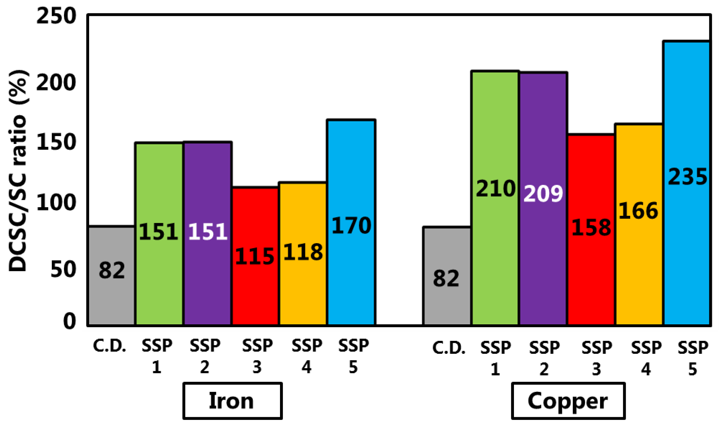
| Iron | Default | 151 | 151 | 115 | 118 | 170 |
| 148 | 149 | 112 | 115 | 167 | ||
| 154 | 154 | 117 | 121 | 173 | ||
| 147 | 148 | 114 | 116 | 164 | ||
| 156 | 155 | 114 | 120 | 176 | ||
| 160 | 158 | 113 | 121 | 182 | ||
| 141 | 143 | 115 | 114 | 157 | ||
| 157 | 149 | 113 | 122 | 177 | ||
| 135 | 151 | 119 | 110 | 152 | ||
| Copper | Default | 210 | 209 | 158 | 166 | 235 |
| 204 | 203 | 153 | 161 | 228 | ||
| 216 | 215 | 163 | 172 | 241 | ||
| 202 | 202 | 158 | 171 | 247 | ||
| 219 | 216 | 156 | 170 | 249 | ||
| 220 | 216 | 156 | 170 | 249 | ||
| 199 | 201 | 161 | 163 | 220 | ||
| 207 | 196 | 152 | 165 | 232 | ||
| 207 | 225 | 169 | 167 | 230 | ||
| Iron | Copper | Iron/Copper (−) | ||
|---|---|---|---|---|
| ADP (kg Sb-e./kg) [65] | 8.43 × 10⁻⁸ | 1.94 × 10⁻³ | 4.35 × 10⁻⁵ | |
| AADP (kg Sb-e./kg) | [26] | 2.38 × 10⁻⁶ | 1.57 × 10⁻³ | 1.52 × 10⁻³ |
| [27] | 2.75 × 10⁻⁸ | 5.41 × 10⁻⁴ | 5.08 × 10⁻⁵ | |
| AADP/ADP ratio (−) | [26] | 28.2 | 0.809 | 34.9 |
| [27] | 0.326 | 0.279 | 1.17 | |
| SC ($/kg) [15] | 7.15 × 10⁻² | 3.05 | 2.34 × 10⁻² | |
| DCSC ($/kg) | C.D. | 5.89 × 10⁻² | 2.49 | 2.37 × 10⁻² |
| SSP1 | 0.108 | 6.41 | 1.69 × 10⁻² | |
| SSP2 | 0.108 | 6.37 | 1.70 × 10⁻² | |
| SSP3 | 8.19 × 10⁻² | 4.82 | 1.70 × 10⁻² | |
| SSP4 | 8.45 × 10⁻² | 5.08 | 1.66 × 10⁻² | |
| SSP5 | 0.122 | 7.16 | 1.70 × 10⁻² | |
| DCSC/SC ratio (−) | C.D. | 0.824 | 0.817 | 1.01 |
| SSP1 | 1.51 | 2.10 | 0.721 | |
| SSP2 | 1.51 | 2.09 | 0.725 | |
| SSP3 | 1.15 | 1.58 | 0.725 | |
| SSP4 | 1.18 | 1.66 | 0.710 | |
| SSP5 | 1.70 | 2.35 | 0.725 | |
© 2018 by the authors. Licensee MDPI, Basel, Switzerland. This article is an open access article distributed under the terms and conditions of the Creative Commons Attribution (CC BY) license (http://creativecommons.org/licenses/by/4.0/).
Share and Cite
Yokoi, R.; Nakatani, J.; Moriguchi, Y. Calculation of Characterization Factors of Mineral Resources Considering Future Primary Resource Use Changes: A Comparison between Iron and Copper. Sustainability 2018, 10, 267. https://0-doi-org.brum.beds.ac.uk/10.3390/su10010267
Yokoi R, Nakatani J, Moriguchi Y. Calculation of Characterization Factors of Mineral Resources Considering Future Primary Resource Use Changes: A Comparison between Iron and Copper. Sustainability. 2018; 10(1):267. https://0-doi-org.brum.beds.ac.uk/10.3390/su10010267
Chicago/Turabian StyleYokoi, Ryosuke, Jun Nakatani, and Yuichi Moriguchi. 2018. "Calculation of Characterization Factors of Mineral Resources Considering Future Primary Resource Use Changes: A Comparison between Iron and Copper" Sustainability 10, no. 1: 267. https://0-doi-org.brum.beds.ac.uk/10.3390/su10010267