Vehicular CO Emission Prediction Using Support Vector Regression Model and GIS


1
Department of Civil Engineering, Faculty of Engineering, University Putra Malaysia, 43400 Serdang, Malaysia
2
RCentre for Advanced Modelling and Geospatial Information Systems (CAMGIS), School of Information, Systems & Modelling (ISM), Faculty of Engineering and Information Technology, University of Technology Sydney, Ultimo, NSW 2007, Australia
3
Department of Energy and Mineral Resources Engineering, Sejong University, Choongmu-gwan, Seoul 209, Korea
*
Author to whom correspondence should be addressed.
Sustainability 2018, 10(10), 3434; https://0-doi-org.brum.beds.ac.uk/10.3390/su10103434
Submission received: 17 July 2018
/
Revised: 24 September 2018
/
Accepted: 25 September 2018
/
Published: 26 September 2018
(This article belongs to the Special Issue Sustainable Applications of Remote Sensing and Geospatial Information Systems to Earth Observations)
Abstract
:Transportation infrastructures play a significant role in the economy as they provide accessibility services to people. Infrastructures such as highways, road networks, and toll plazas are rapidly growing based on changes in transportation modes, which consequently create congestions near toll plaza areas and intersections. These congestions exert negative impacts on human health and the environment because vehicular emissions are considered as the main source of air pollution in urban areas and can cause respiratory and cardiovascular diseases and cancer. In this study, we developed a hybrid model based on the integration of three models, correlation-based feature selection (CFS), support vector regression (SVR), and GIS, to predict vehicular emissions at specific times and locations on roads at microscale levels in an urban areas of Kuala Lumpur, Malaysia. The proposed model comprises three simulation steps: first, the selection of the best predictors based on CFS; second, the prediction of vehicular carbon monoxide (CO) emissions using SVR; and third, the spatial simulation based on maps by using GIS. The proposed model was developed with seven road traffic CO predictors selected via CFS (sum of vehicles, sum of heavy vehicles, heavy vehicle ratio, sum of motorbikes, temperature, wind speed, and elevation). Spatial prediction was conducted based on GIS modelling. The vehicular CO emissions were measured continuously at 15 min intervals (recording 15 min averages) during weekends and weekdays twice per day (daytime, evening-time). The model’s results achieved a validation accuracy of 80.6%, correlation coefficient of 0.9734, mean absolute error of 1.3172 ppm and root mean square error of 2.156 ppm. In addition, the most appropriate parameters of the prediction model were selected based on the CFS model. Overall, the proposed model is a promising tool for traffic CO assessment on roads.
1. Introduction
Transportation infrastructures such as highways, road networks and toll plazas have a great importance in a country’s economy as they provide accessibility services to citizens and merchandise. Building these infrastructures is vital for any developing country. However, road traffic emissions are one of the main sources of air pollution in urban areas because of vehicular exhausts. The high concentrations of traffic emissions have direct and indirect impacts on health and the environment as long-term exposure of these substances can cause respiratory and cardiovascular diseases, preterm births and cancer [1,2,3]. Carbon monoxide (CO) is a toxic air pollutant and is considered as one of the most dangerous pollutants because it has no colour and odour. Carbon monoxide is a product from the incomplete combustion of fuels (e.g., gasoline, oil, natural gas, coal) [4]. As a result, there is a significant need for measuring and estimating the contribution of road traffic emissions to outdoor air pollution in order to establish precise plans for pollution reduction measures and strategies. On roads, highways (high-speed roads), toll gate areas, and intersections, vehicle speed varies based on the traffic condition, which leads to poor urban air quality [5]. Models of road traffic emissions are often used to predict and analyse the level of air pollution on/near roadway links and networks. For example, mathematical simulations, statistical methods, and data mining algorithms are used to analyse road traffic emissions in different regions worldwide [6,7,8].
Although each model has a different purpose, data mining techniques have attracted the interest of numerous policy makers and researchers [9]. However, these models should be designed properly to effectively consider modelling multifactor, uncertainty, and nonlinearity. As measuring traffic emissions on road networks, highways, and toll plazas can be expensive, time-consuming, and dangerous, traffic emission modelling and mapping are important. Furthermore, emissions from road networks and highways cannot be accurately measured during the design stage. When designing new road networks or highways, road traffic emission modelling and mapping such as traffic CO models are needed to provide an expert vision for sustainable planning based on the reduction of pollutant sources such as traffic congestions in highly dense areas. Thus, the spatial modelling and assessment of traffic-emitted CO can facilitate proper planning of environmentally friendly roads.
Many traffic emission assessment models have been reviewed by [10,11,12]. Traditional methods were based on experimental data using gas detectors and simulations. However, they have evolved based on the integration between data sampling techniques and spatial interpolation methods using Geographical Information Systems (GIS) techniques to estimate air pollutant values in uncovered areas. Recently, prediction models have used data mining algorithms with different variables (e.g., land use, road network, traffic data, elevation, and meteorological factors) to predict air pollutant concentrations [13]. However, they are often designed based on experimental data; as a result, each of the models is significantly affected by the composition of uniqueness of the traffic flow and characteristics of the measurement locations. This main disadvantage of road traffic emission prediction models limits their use universally [14]. The models fail to generalise due to local conditions such as vehicle type and weather conditions [15].
2. Previous Works
The literature contains numerous studies conducted using different types of models to predict and simulate road traffic emissions and air quality on roadways such as statistical, regression, spatial, and artificial intelligence models. One of the important models is GIS modelling. Fameli et al. [16] developed a model for predicting traffic emissions by using mathematical equations that depend on statistical information such as fuel consumption and fleet composition. The predicted emissions were graphically represented using GIS techniques (6 × 6 km, 2 × 2 km). Finally, they were compared with experimental data, and the results showed good agreement with the measured data. Dispersion models are also used as effective tools for measuring traffic emissions. Schneider et al. [17] presented an approach based on 3D Eulerian/Lagrangian dispersion model and data sampling by using low-cost sensors to estimate traffic emissions. The traffic flow data and weather information were used as parameters in the presented model. The authors’ model achieved an accuracy of 0.89, and their findings indicated that the proposed approach can provide useful maps based on low-cost sensors. The disadvantages of dispersion models include the expensive applications and data; unrealistic assumptions about dispersion patterns (i.e., Gaussian dispersion); mismatch in the temporal information, which can cause errors in the prediction process; and the high level of experience needed to implement these models [18].
Recently, regression models have attracted considerable attention because of their ability to integrate with the GIS system. Kuai et al. [19] developed a methodology based on geographically weighted regression, least squares regression models that used population, social-economic data, and the geographic data to measure spatial location of healthy food accessibility in Louisiana, USA. Their results indicated that the suburban areas near the cities have better healthy food access than rural areas. Additionally, the socio- economic factors also had a profound impact on the results. Their findings can be useful for helping decision-makers and planners to develop strategies to improve healthy accessibility. In a separate study, Zhao et al. [20] developed an approach by using ordinary least squares regression model and LiDAR data to extract the surface temperature of the buildings roofs in urban areas. Their results showed that there is a significant relationship between the daytime roof temperature and spectral attributes such as slope, aspect, and trees. Whereas, the night-time temperature was only affected by the roof’s spectral attributes and slope.
Ruths et al. [21] designed a local spatio-temporal model based on mobile measurements and a multiple regression algorithm to predict ultrafine particles and black carbon (BC) concentrations emitted from road traffic. Their results indicated a good agreement between the predicted and measured values at the microscale level. However, this model lacked spatial information such as maps. Many commercial models have been used to predict traffic emissions. For example, Borge et al. [22] evaluated traffic emissions (e.g., NOx and PM10) based on a commercial microscale-level simulation model combined with a spatial model. The traffic volume and vehicle speed were used as the model’s parameters. Their results were presented based on the microscale level, grid (5 × 5) m2. This type of model reflects the actual conditions of traffic and the air quality and can be used to support the emission mitigation on hot spot areas. Although this model can effectively predict traffic emissions, it is very costly and requires a high level of experience. The most recent models are the machine learning models, which are widely used in prediction analysis to produce accurate results. Suleiman et al. [8] used the neural network (NN) model to evaluate the impacts of traffic conditions on PM10 concentrations in urban areas based on parameters such as traffic information, road types, and weather information. Their findings indicated that the hourly vehicular emissions were the main factors that contributed to the prediction of PM10. This model can be used as an effective air quality management tool based on various scenarios. Moazami et al. [23] developed a methodology based on uncertainty analysis by using a support vector machine for regression (SVR) model to predict the next day’s concentration of CO. Different datasets were trained to find a suitable dataset to be used in the proposed methodology, which involved weather information and background pollutants such as CH4 and PM10. The authors compared their results with NN models. Their results showed that the SVR model has less uncertainty in CO prediction than the NN model. This methodology can be generalised for modelling in other fields of sciences. The main limitation of this model is the lack of spatial representation of the predicted CO. Nieto et al. [24] presented a method based on SVR technique in an urban area (Northern Spain) at the local scale to predict air pollutants such as NO, CO and PM10 based on historical data. The authors obtained a high correlation coefficient of 0.9088. Although this study showed good agreement between the predicted and the measured concentrations of pollutants at the local scale, it lacked spatial information. In a separate study, Awad et al. [25] developed a model based on the SVR algorithm and big data. They recorded approximately 24,301 samples from 368 monitoring locations to predict fine particle matter and BC. Their results showed good accuracy, which reached up to 87% in the cold season and 79% in the warm season. This model can be utilised in the short- and long-term prediction of BC concentrations. This study presented prediction maps in low-spatial resolution.
Nowadays, the development of computer infrastructure (hardware and software) has led to the creation of a new generation of models called hybrid models. These models improved the performance of traditional models and increased the prediction accuracy. Zhou et al. [26] developed a hybrid model by combining SVR and ant colony optimisation (ACO) to estimate NOx emissions in urban areas. In this study, the optimal model’s parameters were selected based on the ACO model. These optimal parameters increased the prediction accuracy compared with the single SVR model. Sun et al. [27] developed a hybrid model by combining the least square support vector machine (SVM) model and principal component analysis model to predict daily PM2.5 concentrations. Their results showed that the proposed model outperformed the single least square SVM model in the forecasting process. A high correlation of 0.90 for the CO pollutant was recorded. However, this model did not provide a spatial representation of data. Moreover, it required programming skills and high level of experience. In a separate study, Wang et al. [28] developed a hybrid model based on artificial neural network (ANN) and SVM to estimate SO2 and PM2.5 by using historical air quality data and meteorology information recorded from monitoring stations. The study indicated that the application of two stages of prediction approaches can improve the accuracy of air pollution prediction. Although these studies showed the good performance of hybrid models, most of them focused on the statistical results; they neglected the spatial representation of the prediction results. Therefore, several studies were conducted to fill this gap by developing spatial models based on statistical models. Zheng et al. [13] developed a semi-supervised approach by combining the ANN model and linear-chain conditional random field model to produce real-time and fine-grained air quality prediction maps. They used big size of data obtained from air quality monitoring stations for meteorology information. Traffic data were collected based on field surveys using global positioning system techniques by calculating the trajectory of vehicles. By contrast, the land use and road network were extracted from GIS data. The final results were presented based on a spatial grid with spatial resolution of 1 × 1 km2.
However, these models should be designed properly to effectively consider modelling multifactor, uncertainty and nonlinearity. Although many researchers have attempted to solve these issues, they mainly focused on modelling at large areas with big data [29,30,31]. Thus, on-road spatial modelling of traffic emissions (e.g., CO) at the microscale level remains a challenging topic in the transportation field and needs further investigations.
To solve the issues of CO modelling at the microscale level, this study proposes a GIS-based solution considering toll gate locations and characteristics as factors in addition to other factors mentioned in the literature. The proposed model integrates metaheuristic optimisation methods and machine learning models to handle modelling with few examples and avoiding transferability problems. The metaheuristic optimisation such as correlation-based feature selection (CFS) can find the best predictors of CO in a relatively short time compared with other grid search-based methods. On the other hand, machine learning models such as SVM are suitable for modelling with few examples. In addition, integrating these techniques in a single processing pipeline for modelling CO concentrations at highways and toll gate areas is beneficial as the advantages from both methods will be obtained.
The main advantages of the solution are modelling with small data, relatively high accuracy of prediction and the provision of explanation on how traffic emission levels vary at toll gates where workers can become seriously affected. Other advantages include easy implementation in GIS software where users (non-experts) can use for rapid assessment of traffic pollutions. The users can also modify the GIS models to fit their requirements and needs. On the other hand, the integration of metaheuristic optimisation and advanced machine learning models can help improve the prediction of CO concentration levels on highways and toll gate areas. The findings of this work are expected to be useful for decision-makers, transportation agencies and academicians in transportation and environment fields.
3. Materials and Methods
3.1. Study Area
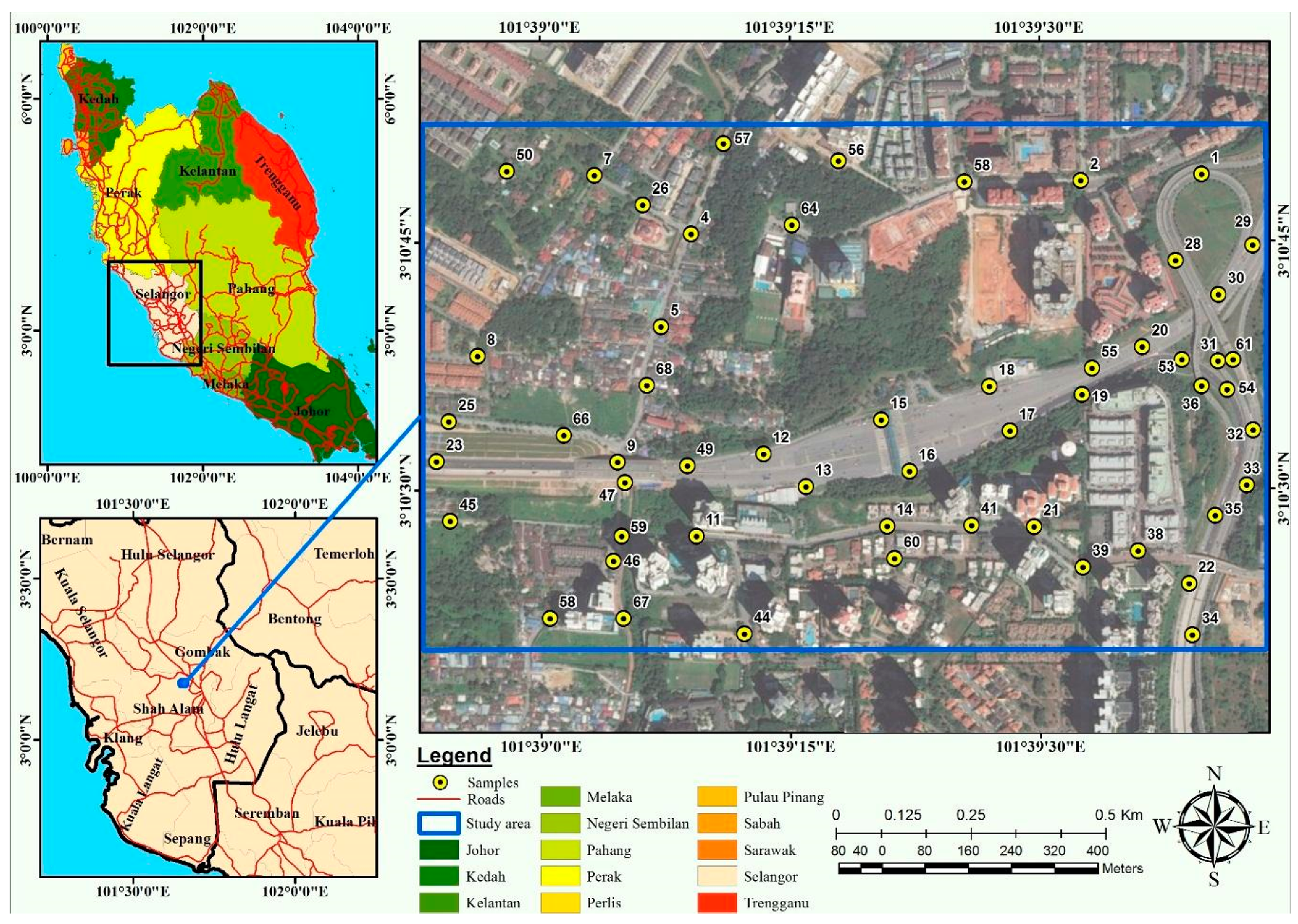
The study area is located near the Jalan Duta toll plaza, which connects the North-South Expressway (NSE) and Duta-Ulu Klang highway. This area falls within a densely populated area in Kuala Lumpur, Malaysia (Figure 1). The NSE is the longest expressway in Malaysia (approximately 772 km in length). It connects the Malaysian–Thai borders and Johor Bahru city. This expressway connects many major cities in the Peninsular Malaysia. Moreover, the NSE is important for trading and tourism activities. The speed limit on the expressway is 110 km/h (68 mph). A study area was selected from the NSE and the surrounding area to achieve the objectives of this study. The selected site contains road network, a toll plaza area, and residential and commercial areas, which make it suitable for traffic emission-related studies.
3.2. Method of CO Measurement
Road traffic CO samples, traffic flow information, and weather data collection are important for comprehensive road traffic CO modelling [32]. Several studies have described methods of collecting traffic data from the site and considered the distribution of air quality samples and their quality as the most important aspect [33,34]. Variations in the traffic CO samples and sampling design significantly affect the accuracy of interpolation at sample locations. Reference [35] stated that point density should be sufficiently high to reach an adequate accuracy of interpolation results. On the other hand, too many points should be avoided to reduce the computation time of the traffic CO software. Most importantly, the density of traffic CO samples should be adjusted considering the traffic CO propagation characteristics. In the current study, the road traffic CO data were collected according to a procedure given by Reference [36]. The method was applied based on spatial analysis by randomly generating traffic CO measurement locations. This procedure creates the optimal number of traffic CO samples compared with the area of the studied region.
Firstly, three layers (i.e., residential, commercial, industrial) from land use were extracted. They were converted into points with a spatial constraint to force generate them inside the land use polygons. Next, the density of points was estimated using a 150 m search radius, and the resolution of output density raster was set to 25 m. Afterwards, the three density rasters were combined using different weights (residential = 3, commercial = 2, industrial = 1). Next, a combined density raster was generated covering the study area. The combined density raster was rescaled by a linear method from 0 to 1, producing the inclusion probability raster to be used to select traffic CO samples in the study area. Then, spatially balanced points were generated within the survey area by utilising the inclusion probability raster. The number of points generated depends on the total length of road networks in the study area. Furthermore, it depends on the cost of the project and the traffic emission instruments involved in data collection. The generated points are distributed within the boundary of the study area. Therefore, additional processing steps were required to refine the generated points to select the final traffic CO samples based on the transportation features. Tessellated grids were generated covering the study area by a grid size of 25 m. The grids that intersect with the generated points and transportation features were selected, and the remaining tessellated grids were removed. Subsequently, the final road traffic CO samples were chosen within the remaining tessellated grids and on transportation features.
3.3. CO Data
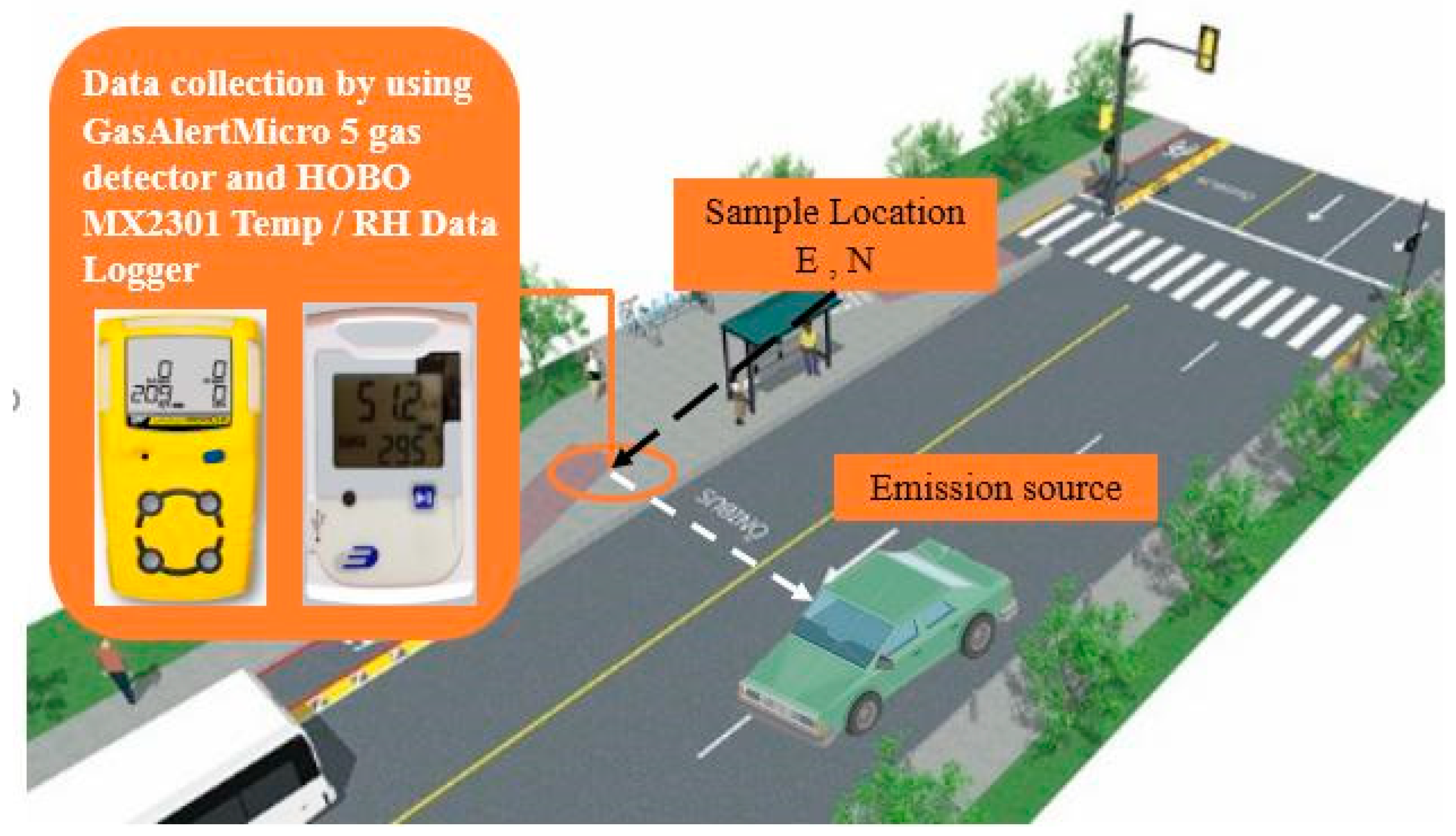
The vehicular CO emissions were observed on the field by using low-cost equipment, GasAlertMicro 5 gas detector/1 ppm resolution and CO measurement precision 0.1 ppm. Traffic flow data and weather information were simultaneously collected using digital cameras for traffic flow information: Data loggers (HOBO MX2301 Temperature/RH Data Logger) with accuracy of +/−0.2 °C and +/−2.5% RH for weather data. Figure 2 shows the sampling procedure. Vehicular CO detectors were installed accurately in the sample locations using GPS equipment. A GPS device (eTrex® 10) was used to observe the coordinates for each sample locations and manually verified using the prepared land use maps. The vehicular CO values were measured two times a day during weekends and weekdays. The vehicular CO emissions were measured during daytime (6:30 a.m. to 8:30 a.m. and 11:30 a.m. to 1:30 p.m.) and evening-time (6:30 p.m. to 8:30 p.m. and 11 p.m. to 12 midnight). In addition, traffic data (i.e., sum of cars, sum of heavy vehicles, and sum of motorbikes) and weather information (i.e., relative humidity, temperature, wind speed, and wind direction) were simultaneously collected with traffic CO concentrations in the study area.
3.4. Vehicular CO Emission Prediction Model
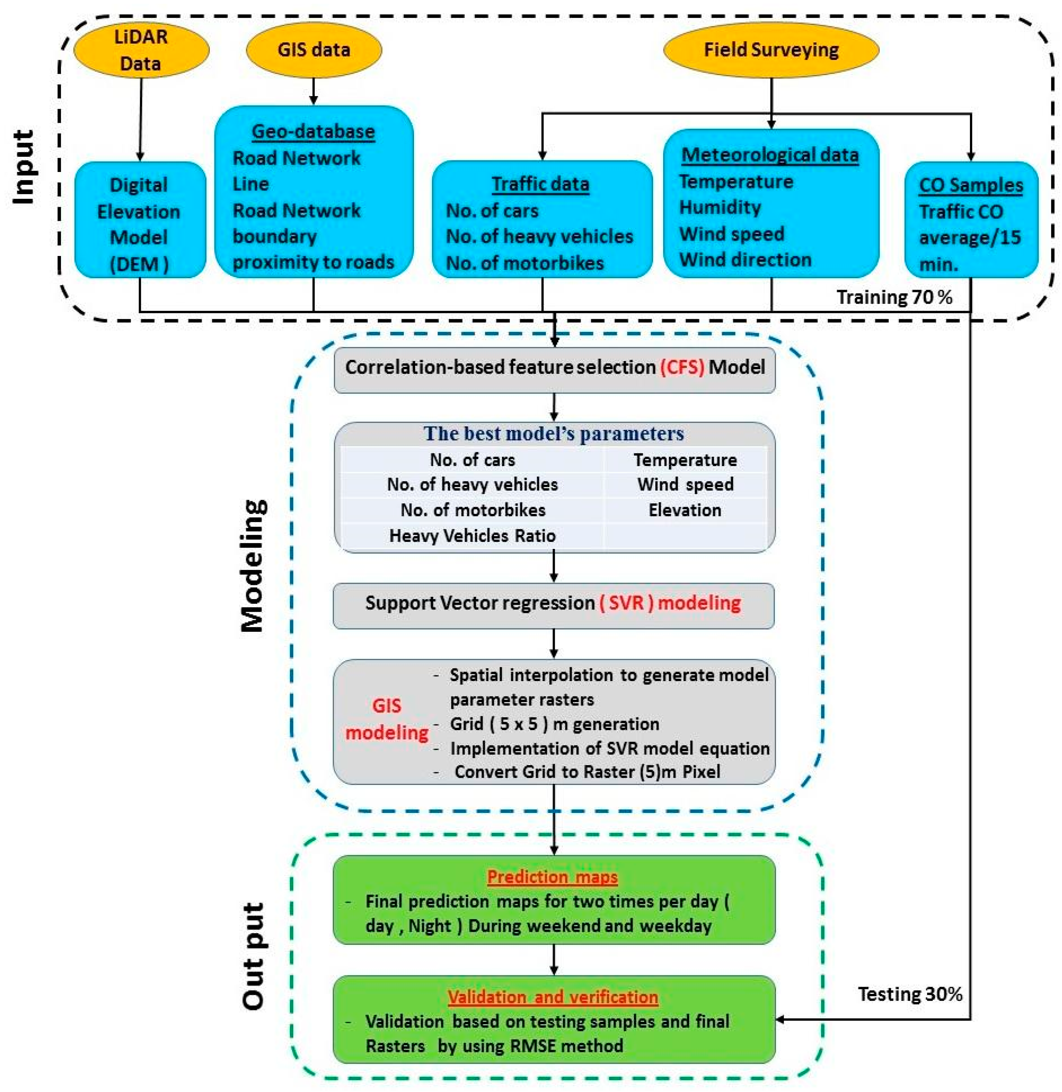
In this section, we will describe the proposed vehicular CO prediction model based on the integration of the SVR model and GIS. The vehicular emission of CO descriptor, weather factors, traffic flow condition and elevation information are explained. Accordingly, SVR is briefly explained, and the proposed structure of the SVR model is presented. The overall methodological flow chart is shown in Figure 3.
3.4.1. Vehicular CO Emission Descriptor and Traffic Parameters
The main purpose of the proposed model is to simulate and predict the CO emitted from vehicles at a specific time and location. Vehicular CO values (the dependent parameter) in this study represent the average of vehicular CO emissions per 15 min [37]. On the other hand, the independent variables were initially determined and selected based on the literature review by taking into account weather and traffic characteristics of the study area. These factors contained the number of cars, car ratio, number of heavy vehicles, ratio of heavy vehicles, number of motorbikes, motorbike ratio, temperature, relative humidity, wind speed, wind direction, proximity to roads, and elevation. These parameters are summarised based on statistics in Table 1. Nonetheless, the model factors may not directly be used as input in the SVR model because some of them may have high correlation with each other, which can generate a multicollinearity problem, a technical problem that could potentially affect any statistical model. Moreover, a large number of model predictors can create an overfitting problem, leading to more complexity in the modelling process. To solve these issues, we developed the model by selecting the relevant and significant factors via statistical approach based on the CFS model.
3.4.2. CFS Model
The CFS model is a famous filter algorithm used for feature selection based on correlation function; it can be implemented based on the free source software WEKA 3.8 [38]. This algorithm is characterised by the selection of subgroups, which contain features that are strongly related to the specified class without any correlation with each other. On the other hand, the features that have low correlation with class ought to be neglected. Moreover, the repetitive features are checked out as they will be exceptionally related with at least one of the other features. The acknowledgement of a feature will depend on the degree to which it predicts classes in territories of the instance space not as of now anticipated by different features.
The assessment function of the CFS’s feature subset is as follows (Equation (1)):
where is the heuristic ‘merit’ of a feature subset S containing k ‘feature class’, is the mean of feature-class correlation (f ∈ S), and is the average of feature-feature intercorrelation.
3.4.3. SVR Model
The SVR model is one of the supervised classification methods used for regression and classification issues based on its significant ability to be universal approximates of multivariate task at any degree of accuracy [39]. This method generalises to solve regression problems [40]. SVR is used to estimate dependent variable based on a set of independents , as shown in Equation (2):
According to the SVR algorithm, the regression model parameters are the noise, which is represented by the error tolerance ), vector of coefficient and the constant . On the other hand, represents the kernel function, which is used to transform the data to the high-dimensional feature space in order to make these data more separable than the original input space. The task is then to find a functional form for . Then, Equations (3)–(5) were obtained based on the tuning of the model. Then, the reduction of error function was used to derive and based on Equations (1) and (2) [41]:
where C indicates a positive constant that determines the degree of penalised loss when a calibration error occurs; N is the sample size; and and are slack variables specifying the upper and lower calibration error subject to ε, respectively [41].
3.5. Proposed Model for Traffic CO Prediction
3.5.1. Proposed CFS-SVR Model
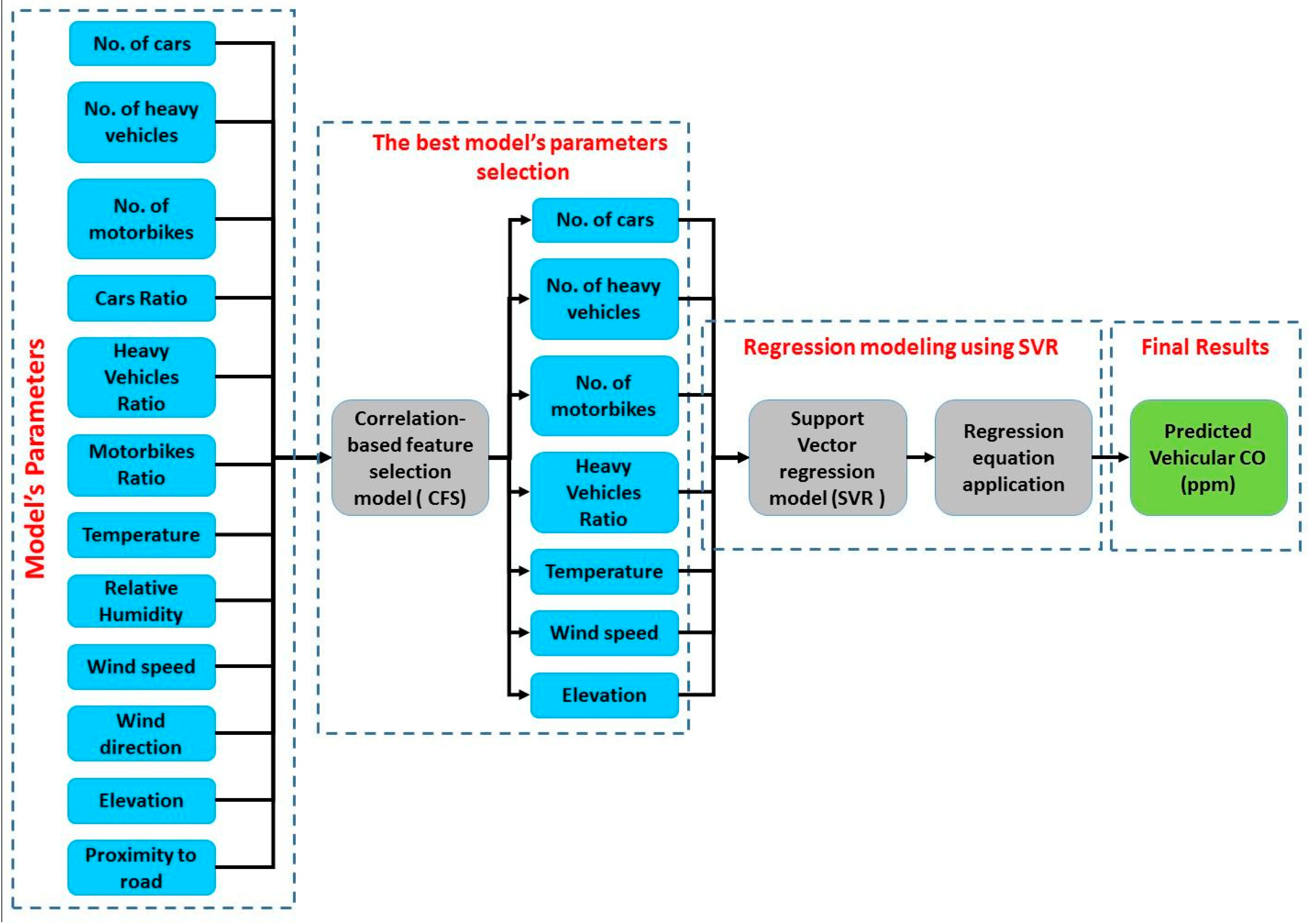
This model was designed (Figure 4) based on the combination of two statistical algorithms: CFS algorithm and SVR model. The first step is to select the model’s most relevant variables. The next step is to apply regression analysis based on SVR model in order to generate final weights, which will help estimate road traffic CO concentrations depending on the model’s parameters. According to the best validation accuracy achieved by a model with seven input parameters instead of 12, the final model architecture was considered for traffic CO prediction in the study area. The optimal parameters are the sum of cars, sum of heavy vehicles, sum of motorbikes, temperature, and relative humidity. The output is the average of the traffic CO concentration (ppm).
The CFS model is an indicator of the relevance power between predictors and the predicted value. It has the ability to rank these predictors and select the best predictors. According to the results, the highest correlation (0.82) was found with the number of heavy vehicles. By contrast, the lowest correlation (0.002) was found with the proximity to roads.
3.5.2. GIS Model
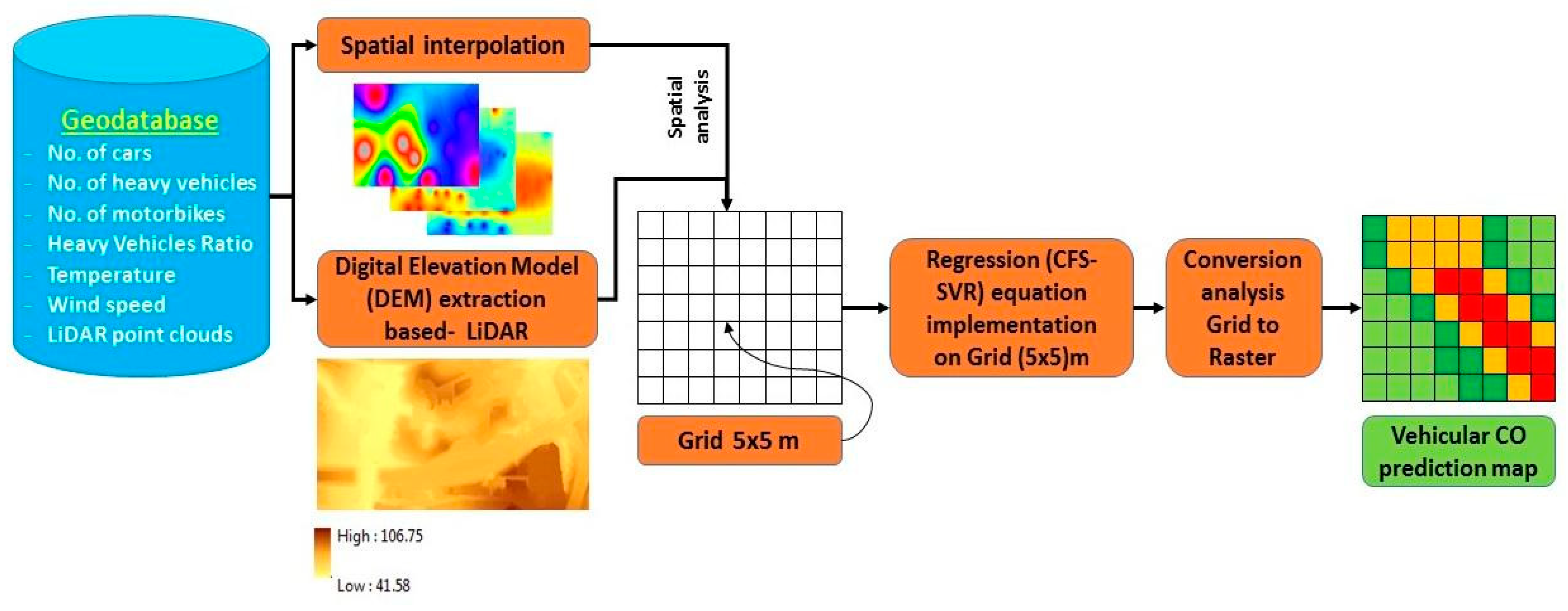
The GIS model (Figure 5) was designed to spatially represent the predicted CO concentrations emitted from traffic on the road network, highway, and toll plaza area. It was designed based on the implementation of the final regression equation resulting from the CFS-SVR model. The model’s parameters were converted from the statistical form into Geodatabase by connecting the samples’ attribute with their locations that were determined using GPS. The parameters were converted to raster form based on geostatistical interpolation (IDW interpolation) for the weather and traffic flow information. We selected the IDW technique because IDW provides a significantly higher degree of correlation than Kriging and Spline methods. On the other hand, the Kriging and Spline results show a higher distortion in the interpolation results than IDW [42]. The elevation information derived from DEM was generated from LiDAR data. The proximity to roads was created based on spatial analysis techniques and the Euclidean distance. The model’s parameters were integrated within GIS environment based on the overlying analysis and the regression equation that was automatically resulted from the CFS-SVR model. They were spatially applied on the high-resolution grid, (5 × 5) m2, to predict the road traffic CO on the unsampled areas. Each grid has value based on the intersected parameter values that will present the variation in traffic CO values and will illustrate the distribution of traffic CO concentration in the study area.
4. Results and Discussions
4.1. CO Prediction Results
4.1.1. Contribution of Vehicular CO Predictors Analysis Using CFS
The developed model parameters have different contribution levels in the average of road vehicular CO emissions in the study area. According to CFS analysis, the model chose seven parameters instead of 12 based on the effectiveness of predictors. The predictors used in the model were temperature, wind speed, number of cars, heavy vehicles, heavy vehicle ratio, number of motorbikes, and elevation. Statistics indicated that these parameters were the best for predicting traffic CO variation in the dataset. Overall, the emitted CO was highly correlated with traffic volume data.
4.1.2. Results of Vehicular CO Prediction Model (CFS-SVR)
Two SVR models were trained and validated. The first model was trained without combining with the CFS model based on 12 parameters (i.e., number of vehicles, number of heavy vehicles, number of motorbikes, car ratio, heavy vehicle ratio, motorbike ratio, temperature, humidity, wind speed, wind direction, DEM, and proximity to roads) to produce the predicted CO concentration. The second model was trained by combining both the SVR and CFS models with only seven parameters that resulted from the CFS model (number of vehicles, number of heavy vehicles, number of motorbikes, heavy vehicle ratio, motorbike ratio, temperature, wind speed, and DEM). The CFS model was utilised to increase the accuracy of the SVR model results by selecting the best parameters to predict the traffic CO in the study area. Table 2 shows the comparison between results before and after the combination between the SVR model and the CFS model. According to the training results, the results of the SVR model were improved based on the combination with the CFS model. The validation results showed that SVR produced 69% and CFS-SVR produced 78%.
4.2. Results of the Spatial Prediction of Vehicular CO
The final regression equation was created by using the proposed model (CFS-SVR) based on the sum of the collected data during weekends and weekdays (daytime, night-time) to generate coefficients of the model’s parameters. This equation was used to simulate prediction maps at daytime and night-time during weekends and weekdays. The SVR equation shown below (Equation (6)) was based on the integration between CFS and SVR models:
Road = − 0.008 × Temperature + 0.0472 × Wind speed + 0.0117 × cars + 0.0636 × Heavy vehicle + 0.0042 × Heavy vehicle ratio + 0.0004× motorbike – 0.0184 × Elevation + 2.0789
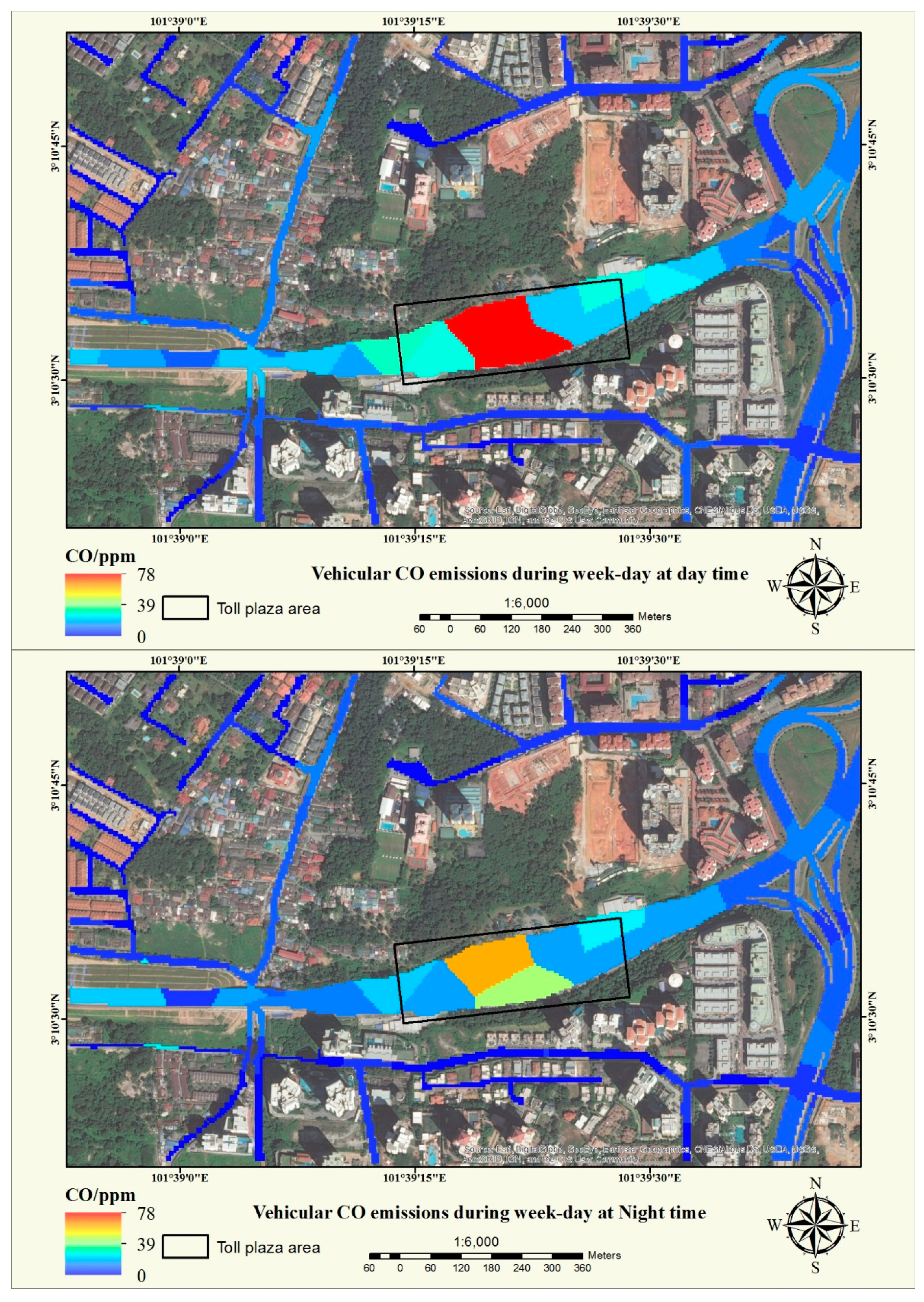
GIS modelling was applied based on the developed regression equation and the model’s parameters multiplied by their coefficients and their locations on the map by using a very high-resolution grid, (5 × 5) m2. GIS modelling was used to produce prediction maps (Figure 6 and Figure 7) at the microscale level, at different times per day (daytime, night-time) during weekdays and weekends. The prediction maps (Figure 6 and Figure 7) showed that the vehicular CO emission values were very high during weekdays because of traffic congestions that occurred at peak hours in the morning compared with those recorded during daytime through a normal traffic flow. Meanwhile, the highest vehicular CO concentration during weekdays at daytime was 78 ppm, which decreased to 11.8 ppm during weekends at day time. On the other hand, the highest value at night-time was recorded during weekdays (63.5 ppm) and weekends (36 ppm). From the prediction maps, the vehicular CO spatial distribution is more concentrated near the toll plaza area than other areas because of the heavy traffic congestion at toll gates. However, the lowest vehicular CO values can be seen closer to residential areas than highways and major roads, which reached 0 ppm or closer to 0 ppm. The modelling results showed a significant variation in the vehicular CO values between the weekends and weekdays, indicating that there is a high correlation between traffic congestions and vehicular CO values. The vehicular emissions increased because of traffic congestions.
4.3. Validation of the CO Prediction Maps
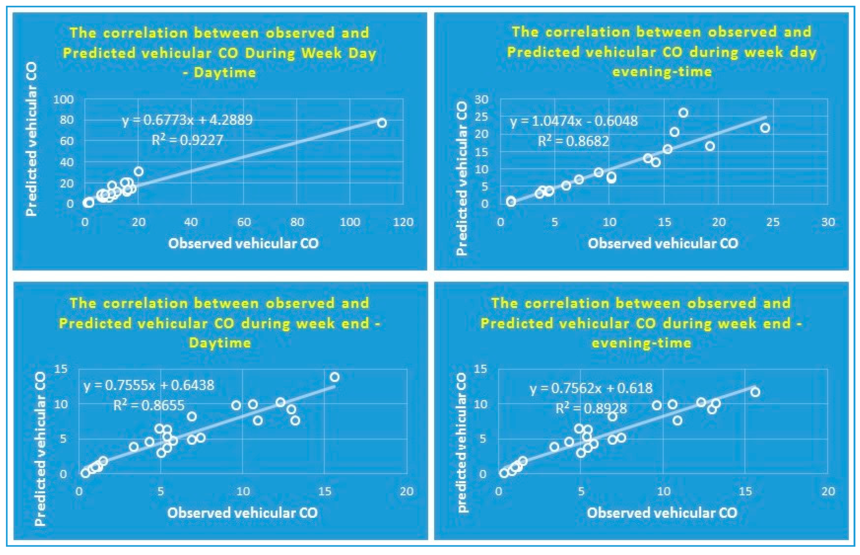
The validation process was applied based on root mean square error (RMSE) and testing data. The predicted values were compared with the observed values (Figure 8). According to the testing data, the correlation coefficient was 0.9345, the mean absolute error (MAE) was 1.44 ppm, and RMSE was 2.37 ppm. The lowest correlation between predicted and measured values was calculated during weekends at daytime (which was 86%), and the highest correlation obtained was 92% during the work day at daytime.
4.4. Comparison with Other Models
A comparative analysis was conducted between CFS-SVR and a linear regression (LR) model, which is considered a simple model and does not require a high level of experience for implementation. The LR model generated a statistical equation based on the total input parameters and the selected parameters based on the CFS model. The LR model is shown in Equation (7).
Traffic CO = 0.11 × Number of heavy vehicles + 4.62
Table 3 shows the comparison results between the CFS-SVR model and the LR model based on the training dataset. The results showed that the proposed model had a better performance than the LR model. The correlation coefficient based on the LR model was 0.9191, MAE was 2.9067 ppm, RMSE was 3.7032 ppm, relative absolute error was 52.68%, and root relative square error was 39.39%. Figure 9 shows the comparison amongst the three models (developed CFS-SVR model, traditional model, and simple LR model), where the highest RMSE was detected in the LR model (12.2 ppm), and the lowest value was detected in the CFS-SVR model (0.008 ppm).
5. Conclusions
Vehicular emissions (e.g., CO) are one of the major sources of environmental pollution in urban areas, where road networks, intersections, and toll plaza areas are present. Vehicular emission prediction models and spatial models are used to assess the impacts of vehicular emissions from different types of vehicles on human health and the environment. In this study, a hybrid model was developed based on the integration of three models: CFS, SVR, and GIS. The hybrid model could accurately predict the vehicular CO (80.6) and obtained the lowest RMSE (2.156 ppm). The default model parameters were 12 parameters. After the implementation of the CFS model, the model eliminated the proximity to roads, car ratio, motorbike ratio, relative humidity, and wind direction as factors, because they were not correlated with CO.
GIS modelling was applied based on the parameters derived from LiDAR data, and GIS layers were extracted from interpolation techniques to produce prediction maps for different times per day at the microscale in the study area. The simulated vehicular CO concentrations ranged from 78 ppm near the toll plaza area to 0 ppm far away from the toll area. According to the prediction maps, a spatial variation was detected between traffic CO concentrations, where the highest values were concentrated near highly congested areas, whilst the lowest values were distributed far away from areas with traffic activities.
Both vehicular CO statistical modelling and GIS techniques are important tools for transportation planning and traffic emission evaluation. Prediction maps can be efficiently used as decision-making tools in order to propose suitable solutions for reducing traffic jams in toll plaza areas, highways, and road networks. For example, in toll plaza management, advanced systems can be used instead of the current ones. As vehicular emission pollution assessment by governmental or private agencies is very complex and expensive due to the requirements of experts and advanced systems, the proposed models are inexpensive and easy to apply for assessing vehicular CO impacts. Moreover, vehicular CO pollution levels change based on traffic conditions and the number of vehicles. Therefore, periodic assessment of vehicular emissions through governmental or private agencies is required. On the other hand, selecting the parameter simulations of the best model is very effective to mitigate data collection works, which saves time, cost, and efforts. Moreover, it can reduce the computation time. On the other hand, GIS modelling is useful for non-expert users to perform traffic CO impact assessment in different applications. The limitation of this study was the complexity of data collection from the field. This type of models can be developed by applying the most recent techniques, such as deep learning algorithms, to improve the accuracy of the prediction results.
Author Contributions
B.P. conceptualised, supervised, and obtained the grant for the study. B.P. and O.S.A. collected and analysed the data, performed the analyses and validation, wrote the manuscript and contributed to the re-structuring and editing of the manuscript. B.P., O.S.A. and H.Z.M.S. professionally optimised the manuscript.
Funding
This research is supported by the UTS under grant number 321740.2232335 and 321740.2232357.
Acknowledgments
The authors acknowledge and appreciate the provision of LiDAR data, satellite images, and logistic support by PLUS Berhad. In addition, the authors gratefully acknowledge the financial support from the UPM-PLUS industry project grant.
Conflicts of Interest
The authors declare no conflict of interest.
References
- Garshick, E.; Laden, F.; Hart, J.E.; Caron, A. Residence near a major road and respiratory symptoms in US veterans. Epidemiology 2003, 14, 728–736. [Google Scholar] [CrossRef] [PubMed]
- Delfino, R.; Tjoa, T.; Gillen, D.L.; Staimer, N.; Polidori, A.; Arhami, M.; Jamner, L.; Sioutas, C.; Longhurst, J. Traffic-related air pollution and blood pressure in elderly subjects with coronary artery disease. Epidemiology 2010, 21, 396–404. [Google Scholar] [CrossRef] [PubMed]
- Crouse, D.L.; Goldberg, M.S.; Ross, N.A.; Chen, H.; Labrèche, F. Postmenopausal breast cancer is associated with exposure to traffic-related air pollution in Montreal, Canada: A case–control study. Environ. Health Perspect. 2010, 118, 1578–1583. [Google Scholar] [PubMed]
- Brook, R.D.; Franklin, B.; Cascio, W.; Hong, Y.; Howard, G.; Lipsett, M.; Luepker, R.; Mittleman, M.; Samet, J.; Smith, S.C., Jr.; et al. Air pollution and cardiovascular disease: A statement for healthcare professionals from the Expert Panel on Population and Prevention Science of the American Heart Association. Circulation 2004, 109, 2655–2671. [Google Scholar] [PubMed]
- Pandian, S.; Gokhale, S.; Ghoshal, A.K. Evaluating effects of traffic and vehicle characteristics on vehicular emissions near traffic intersections. Transp. Res. Part D Transp. Environ. 2009, 14, 180–196. [Google Scholar]
- Zhou, X.; Tanvir, S.; Lei, H.; Taylor, J.; Liu, B.; Rouphail, N.M.; Frey, H.C. Integrating a simplified emission estimation model and mesoscopic dynamic traffic simulator to efficiently evaluate emission impacts of traffic management strategies. Transp. Res. Part D Transp. Environ. 2015, 37, 123–136. [Google Scholar]
- Yazdi, M.N.; Delavarrafiee, M.; Arhami, M. Evaluating near highway air pollutant levels and estimating emission factors: Case study of Tehran, Iran. Sci. Total Environ. 2015, 538, 375–384. [Google Scholar] [CrossRef] [PubMed]
- Suleiman, A.; Tight, M.R.; Quinn, A.D. Assessment and prediction of the impact of road transport on ambient concentrations of particulate matter PM10. Transp. Res. Part D Transp. Environ. 2016, 49, 301–312. [Google Scholar]
- Cai, M.; Yin, Y.; Xie, M. Prediction of hourly air pollutant concentrations near urban arterials using artificial neural network approach. Transp. Res. Part D Transp. Environ. 2009, 14, 32–41. [Google Scholar] [CrossRef]
- Singh, D.; Kumar, A.; Kumar, K.; Singh, B.; Mina, U.; Singh, B.B.; Jain, V.K. Statistical modeling of O3, NOx, CO, PM2.5, VOCs and noise levels in commercial complex and associated health risk assessment in an academic institution. Sci. Total Environ. 2016, 572, 586–594. [Google Scholar] [CrossRef] [PubMed]
- Behera, S.N.; Sharma, M.; Mishra, P.K.; Nayak, P.; Damez-Fontaine, B.; Tahon, R. Passive measurement of NO2 and application of GIS to generate spatially-distributed air monitoring network in urban environment. Urban Clim. 2015, 14, 396–413. [Google Scholar] [CrossRef]
- Johnson, M.; Isakov, V.; Touma, J.S.; Mukerjee, S.; Özkaynak, H. Evaluation of land-use regression models used to predict air quality concentrations in an urban area. Atmos. Environ. 2010, 44, 3660–3668. [Google Scholar] [CrossRef]
- Zheng, Y.; Liu, F.; Hsieh, H.P. U-Air: When Urban Air Quality Inference Meets Big Data. In Proceedings of the 19th ACM SIGKDD International Conference on Knowledge Discovery and Data Mining, Chicago, IL, USA, 11–14 August 2013; pp. 1436–1444. [Google Scholar]
- Tomić, J.; Bogojević, N.; Pljakić, M.; Šumarac-Pavlović, D. Assessment of traffic noise levels in urban areas using different soft computing techniques. J. Acoust. Soc. Am. 2016, 40, EL340–EL345. [Google Scholar] [CrossRef] [PubMed]
- Hamad, K.; Khalil, M.A.; Shanableh, A. Modeling roadway traffic noise in a hot climate using artificial neural networks. Transp. Res. Part D Transp. Environ. 2017, 53, 161–177. [Google Scholar] [CrossRef]
- Fameli, K.M.; Assimakopoulos, V.D. Development of a road transport emission inventory for Greece and the Greater Athens Area: Effects of important parameters. Sci. Total Environ. 2015, 505, 770–786. [Google Scholar] [CrossRef] [PubMed] [Green Version]
- Schneider, P.; Castell, N.; Vogt, M.; Dauge, F.R.; Lahoz, W.A.; Bartonova, A. Mapping urban air quality in near real-time using observations from low-cost sensors and model information. Environ. Int. 2017, 106, 234–247. [Google Scholar] [CrossRef] [PubMed]
- Jerrett, M.; Arain, A.; Kanaroglou, P.; Beckerman, B.; Potoglou, D.; Sahsuvaroglu, T.; Morrison, J.; Giovis, C. A review and evaluation of intraurban air pollution exposure models. J. Expo. Sci. Environ. Epidemiol. 2005, 15, 185–204. [Google Scholar] [CrossRef] [PubMed]
- Kuai, X.; Zhao, Q. Examining healthy food accessibility and disparity in Baton Rouge, Louisiana. Ann. GIS 2017, 23, 103–116. [Google Scholar] [CrossRef]
- Zhao, Q.; Myint, S.; Wentz, E.; Fan, C. Rooftop surface temperature analysis in an urban residential environment. Remote Sens. 2015, 7, 12135–12159. [Google Scholar] [CrossRef]
- Ruths, M.; von Bismarck-Osten, C.; Weber, S. Measuring and modelling the local-scale spatio-temporal variation of urban particle number size distributions and black carbon. Atmos. Environ. 2014, 96, 37–49. [Google Scholar] [CrossRef]
- Borge, R.; Narros, A.; Artíñano, B.; Yagüe, C.; Gómez-Moreno, F.J.; de la Paz, D.; Román-Cascón, C.; Díaz, E.; Maqueda, G.; Sastre, M.; et al. Assessment of microscale spatio-temporal variation of air pollution at an urban hotspot in Madrid (Spain) through an extensive field campaign. Atmos. Environ. 2016, 140, 432–445. [Google Scholar] [CrossRef]
- Moazami, S.; Noori, R.; Amiri, B.J.; Yeganeh, B.; Partani, S.; Safavi, S. Reliable prediction of carbon monoxide using developed support vector machine. Atmos. Pollut. Res. 2016, 7, 412–418. [Google Scholar] [CrossRef]
- Nieto, P.G.; Combarro, E.F.; del Coz Díaz, J.J.; Montañés, E. A SVM-based regression model to study the air quality at local scale in Oviedo urban area (Northern Spain): A case study. Appl. Math. Comput. 2013, 219, 8923–8937. [Google Scholar]
- Awad, Y.A.; Koutrakis, P.; Coull, B.A.; Schwartz, J. A spatio-temporal prediction model based on support vector machine regression: Ambient Black Carbon in three New England States. Environ. Res. 2017, 159, 427–434. [Google Scholar] [CrossRef] [PubMed]
- Zhou, H.; Zhao, J.P.; Zheng, L.G.; Wang, C.L.; Cen, K.F. Modeling NOx emissions from coal-fired utility boilers using support vector regression with ant colony optimization. Eng. Appl. Artif. Intell. 2012, 25, 147–158. [Google Scholar] [CrossRef]
- Sun, W.; Sun, J. Daily PM2.5 concentration prediction based on principal component analysis and LSSVM optimized by cuckoo search algorithm. J. Environ. Manag. 2017, 188, 144–152. [Google Scholar] [CrossRef] [PubMed]
- Wang, P.; Liu, Y.; Qin, Z.; Zhang, G. A novel hybrid forecasting model for PM10 and SO2 daily concentrations. Sci. Total Environ. 2015, 505, 1202–1212. [Google Scholar] [CrossRef] [PubMed]
- Corani, G. Air quality prediction in Milan: Feed-forward neural networks, pruned neural networks and lazy learning. Ecol. Modell. 2005, 185, 513–529. [Google Scholar] [CrossRef]
- Singh, K.P.; Gupta, S.; Rai, P. Identifying pollution sources and predicting urban air quality using ensemble learning methods. Atmos. Environ. 2013, 80, 426–437. [Google Scholar] [CrossRef]
- Weichenthal, S.; Van Ryswyk, K.; Goldstein, A.; Bagg, S.; Shekkarizfard, M.; Hatzopoulou, M. A land use regression model for ambient ultrafine particles in Montreal, Canada: A comparison of linear regression and a machine learning approach. Environ. Res. 2016, 146, 65–72. [Google Scholar] [CrossRef] [PubMed] [Green Version]
- Namdeo, A.; Mitchell, G.; Dixon, R. TEMMS: An integrated package for modelling and mapping urban traffic emissions and air quality. Environ. Modell. Softw. 2002, 17, 177–188. [Google Scholar] [CrossRef]
- Kho, F.W.; Law, P.L.; Ibrahim, S.H.; Sentian, J. Carbon monoxide levels along roadway. Int. J. Environ. Sci. Technol. 2007, 4, 27–34. [Google Scholar] [CrossRef] [Green Version]
- Ranjbar, H.R.; Gharagozlou, A.R.; Nejad, A.R. 3D analysis and investigation of traffic noise impact from Hemmat highway located in Tehran on buildings and surrounding areas. J. Geogr. Inf. Syst. 2012, 4, 322–334. [Google Scholar] [CrossRef]
- Li, F.; Liao, S.S.; Cai, M. A new probability statistical model for traffic noise prediction on free flow roads and control flow roads. Transp. Res. Part D Transp. Environ. 2016, 49, 313–322. [Google Scholar] [CrossRef]
- Ragettli, M.S.; Goudreau, S.; Plante, C.; Fournier, M.; Hatzopoulou, M.; Perron, S.; Smargiassi, A. Statistical modeling of the spatial variability of environmental noise levels in Montreal, Canada, using noise measurements and land use characteristics. J. Expo. Sci. Environ. Epidemiol. 2016, 26, 597–605. [Google Scholar] [CrossRef] [PubMed]
- Dekoninck, L.; Botteldooren, D.; Panis, L.I.; Hankey, S.; Jain, G.; Karthik, S.; Marshall, J. Applicability of a noise-based model to estimate in-traffic exposure to black carbon and particle number concentrations in different cultures. Environ. Int. 2015, 74, 89–98. [Google Scholar] [CrossRef] [PubMed] [Green Version]
- Hall, M.A. Correlation-Based Feature Selection for Machine Learning. Ph.D. Thesis, The University of Waikato, Hamilton, New Zealand, 1999. [Google Scholar]
- Bishop, C.M. Pattern Recognition and Machine Learning; Springer: New York, NY, USA, 2006. [Google Scholar]
- Schölkopf, B.; Bartlett, P.L.; Smola, A.J.; Williamson, R.C. Shrinking the Tube: A New Support Vector Regression Algorithm. In Advances in Neural Information Processing Systems; MIT Press: London, UK, 1999; pp. 330–336. [Google Scholar]
- Goel, A.; Pal, M. Application of support vector machines in scour prediction on grade-control structures. Eng. Appl. Artif. Intell. 2009, 22, 216–223. [Google Scholar] [CrossRef]
- Gong, G.; Mattevada, S.; O’bryant, S.E. Comparison of the accuracy of kriging and IDW interpolations in estimating groundwater arsenic concentrations in Texas. Environ. Res. 2014, 130, 59–69. [Google Scholar] [CrossRef] [PubMed]
Figure 1.
Location map of the chosen sites.

Figure 2.
Vehicular CO and meteorological data measurement on roadway section.

Figure 3.
Overall methodology.

Figure 4.
Proposed correlation-based feature selection - support vector regression (CFS-SVR) model.

Figure 5.
Proposed GIS model.

Figure 6.
Prediction maps during weekends (daytime, evening-time).

Figure 7.
Prediction maps during weekdays (daytime, evening-time).

Figure 8.
Correlation between observed and predicted vehicular CO based on different times.

Figure 9.
Comparison between the models.


Table 1.
Summary statistics of CO emission predictors.
| Parameters | Weekends | Weekdays | ||||||
|---|---|---|---|---|---|---|---|---|
| Mean | Min. | Max. | Std. Dev. | Mean | Min. | Max. | Std. Dev. | |
| Sum of cars (per 15 min) | 353.9 | 0 | 1793 | 298.91 | 597.25 | 0 | 2800 | 488.56 |
| Sum of heavy vehicles (per 15 min) | 17.48 | 0 | 220 | 24.14 | 53.82 | 0 | 760 | 106.24 |
| Sum of motorbikes (per 15 min) | 26.62 | 0 | 112 | 21.54 | 36.75 | 0 | 242 | 35.29 |
| Temperature (°C) | 29.3 | 26 | 34.33 | 2.32 | 29.39 | 24 | 33.8 | 2.79 |
| Relative humidity (%) | 81.61 | 56 | 94.8 | 13.05 | 76.16 | 50.4 | 94.9 | 16.3 |
| Wind speed (mph) | 4.55 | 0 | 11 | 3.07 | 3.87 | 0 | 7 | 2.22 |
| Wind direction (angle/0° N, 90° E, 270° W, 180° S) | 136 | 0 | 350 | 116.24 | 165 | 0 | 360 | 117 |
| Digital Elevation Model (DEM) (m) | 66.2 | 41.58 | 106.75 | 12.8 | 66.2 | 41.58 | 106.75 | 12.8 |
| Proximity to roads (m) | 11.16 | 3 | 174.02 | 26.13 | 11.16 | 3 | 174.02 | 26.13 |
Table 2.
Comparison between results before and after the combination of the SVR model and CFS model.
Table 2.
Comparison between results before and after the combination of the SVR model and CFS model.
| SVR Model | CFS-SVR Model | ||
|---|---|---|---|
| No. of parameters | 12 | No. of parameters | 7 |
| Correlation coefficient | 0.9675 | Correlation coefficient | 0.9734 |
| Mean absolute error | 1.4337 | Mean absolute error | 1.3172 |
| Root mean square error | 2.4449 | Root mean square error | 2.156 |
| Relative absolute error | 25.73% | Relative absolute error | 23.87% |
| Root relative square error | 25.82% | Root relative square error | 22.93% |
| Total number of instances | 196 | Total number of instances | 196 |
Table 3.
Comparison of results between the CFS-SVR model and LR model.
| CFS-SVR Model | LR Model | ||
|---|---|---|---|
| Correlation coefficient | 0.9734 | Correlation coefficient | 0.9191 |
| Mean absolute error | 1.3172 | Mean absolute error | 2.9067 |
| Root mean square error | 2.156 | Root mean square error | 3.7032 |
| Relative absolute error | 23.87% | Relative absolute error | 52.68% |
| Root relative square error | 22.93% | Root relative square error | 39.39% |
| Total number of instances | 196 | Total number of instances | 196 |
© 2018 by the authors. Licensee MDPI, Basel, Switzerland. This article is an open access article distributed under the terms and conditions of the Creative Commons Attribution (CC BY) license (http://creativecommons.org/licenses/by/4.0/).
Share and Cite
MDPI and ACS Style
Azeez, O.S.; Pradhan, B.; Shafri, H.Z.M. Vehicular CO Emission Prediction Using Support Vector Regression Model and GIS. Sustainability 2018, 10, 3434. https://0-doi-org.brum.beds.ac.uk/10.3390/su10103434
AMA Style
Azeez OS, Pradhan B, Shafri HZM. Vehicular CO Emission Prediction Using Support Vector Regression Model and GIS. Sustainability. 2018; 10(10):3434. https://0-doi-org.brum.beds.ac.uk/10.3390/su10103434
Chicago/Turabian StyleAzeez, Omer Saud, Biswajeet Pradhan, and Helmi Z. M. Shafri. 2018. "Vehicular CO Emission Prediction Using Support Vector Regression Model and GIS" Sustainability 10, no. 10: 3434. https://0-doi-org.brum.beds.ac.uk/10.3390/su10103434
Note that from the first issue of 2016, this journal uses article numbers instead of page numbers. See further details here.